cva / dva / fva - analytical finance - by jan römanjanroman.dhis.org/finance/xva/cva_dva_fva...
TRANSCRIPT
1
CVA / DVA / FVA
a comprehensive approach
under stressed markets
Gary Wong
2
References
• C. Albanese, S. Iabichino: The FVA-DVA puzzle:
completing market with collateral trading strategies,
available on www.albanese.co.uk
• John hull and Alan White: Valuing Derivatives:
Funding Value Adjustments and Fair Value, working
paper, Sept 2013
• C. Albanese, D. Brigo, F. Oertel: Restructuring
counterparty credit risk, to appear on IJTAF and in the
Working Paper Series of the Bundesbank, SSRN
1969344 (2011)
• C. Albanese, G. Pietronero: A redesign for central
clearing, Credit Flux, August 2011
3
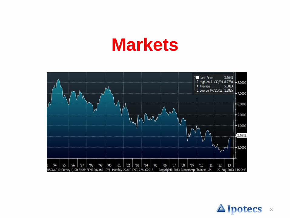
Markets
4
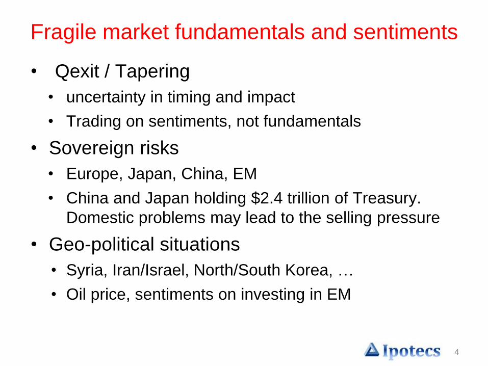
Fragile market fundamentals and sentiments
• Qexit / Tapering
• uncertainty in timing and impact
• Trading on sentiments, not fundamentals
• Sovereign risks
• Europe, Japan, China, EM
• China and Japan holding $2.4 trillion of Treasury.
Domestic problems may lead to the selling pressure
• Geo-political situations
• Syria, Iran/Israel, North/South Korea, …
• Oil price, sentiments on investing in EM
5
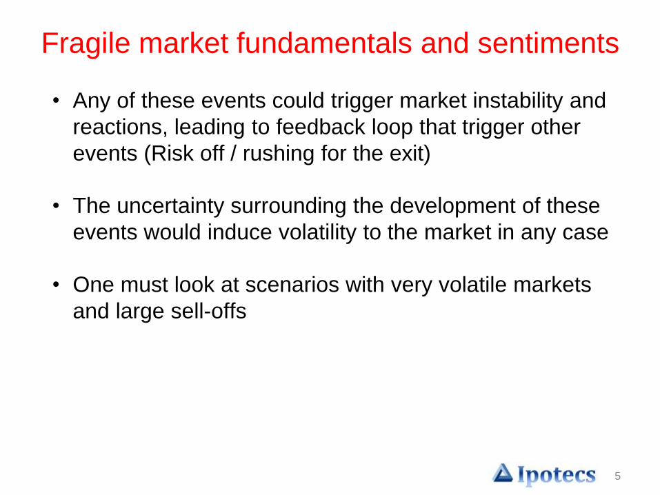
Fragile market fundamentals and sentiments
• Any of these events could trigger market instability and
reactions, leading to feedback loop that trigger other
events (Risk off / rushing for the exit)
• The uncertainty surrounding the development of these
events would induce volatility to the market in any case
• One must look at scenarios with very volatile markets
and large sell-offs
6
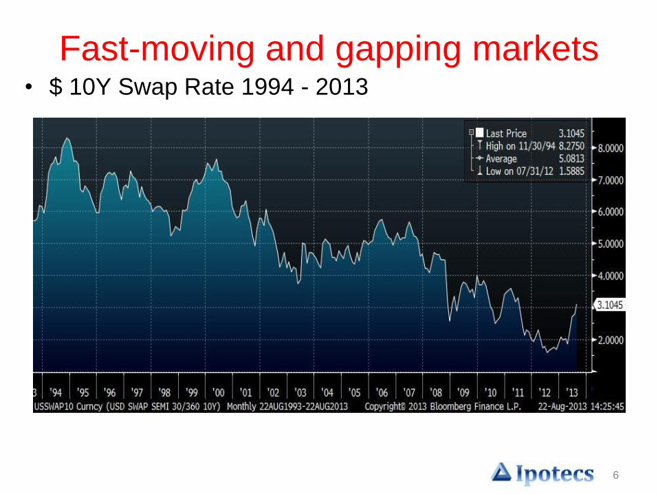
Fast-moving and gapping markets • $ 10Y Swap Rate 1994 - 2013
7
Collateral, CVA, DVA and FVAunder fast and gapping markets
8
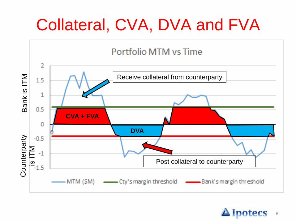
Collateral, CVA, DVA and FVAB
ank is IT
MC
ounte
rpart
y
is IT
M
DVA
Receive collateral from counterparty
CVA + FVA
Post collateral to counterparty
9
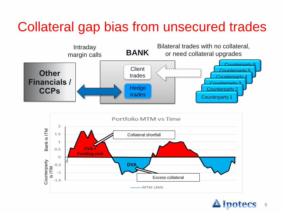
Collateral gap bias from unsecured trades
Counterparty 6
Counterparty 5
Counterparty 4
Counterparty 3
Counterparty 2
Counterparty 1
Other Financials /
CCPs
Bilateral trades with no collateral,
or need collateral upgrades
Client
trades
Hedge
trades
BANKIntraday
margin calls
Ba
nk is I
TM
Co
un
terp
art
y
is I
TM
CVA +
Funding cost
DVA
Collateral shortfall
Excess collateral
10
Collateral
11
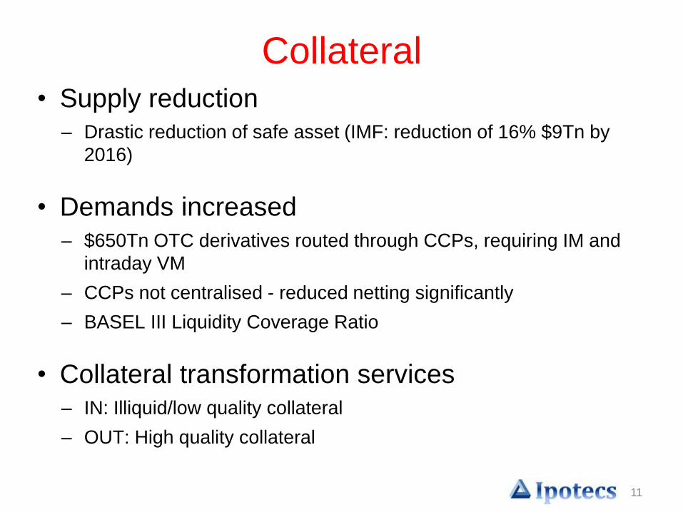
Collateral• Supply reduction
– Drastic reduction of safe asset (IMF: reduction of 16% $9Tn by
2016)
• Demands increased
– $650Tn OTC derivatives routed through CCPs, requiring IM and
intraday VM
– CCPs not centralised - reduced netting significantly
– BASEL III Liquidity Coverage Ratio
• Collateral transformation services
– IN: Illiquid/low quality collateral
– OUT: High quality collateral
12
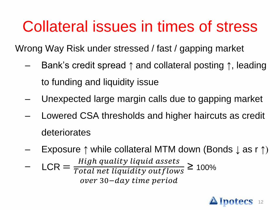
Collateral issues in times of stress
Wrong Way Risk under stressed / fast / gapping market
– Bank’s credit spread ↑ and collateral posting ↑, leading
to funding and liquidity issue
– Unexpected large margin calls due to gapping market
– Lowered CSA thresholds and higher haircuts as credit
deteriorates
– Exposure ↑ while collateral MTM down (Bonds ↓ as r ↑)
– LCR=𝐻𝑖𝑔ℎ 𝑞𝑢𝑎𝑙𝑖𝑡𝑦 𝑙𝑖𝑞𝑢𝑖𝑑 𝑎𝑠𝑠𝑒𝑡𝑠𝑇𝑜𝑡𝑎𝑙 𝑛𝑒𝑡 𝑙𝑖𝑞𝑢𝑖𝑑𝑖𝑡𝑦 𝑜𝑢𝑡𝑓𝑙𝑜𝑤𝑠𝑜𝑣𝑒𝑟 30−𝑑𝑎𝑦 𝑡𝑖𝑚𝑒 𝑝𝑒𝑟𝑖𝑜𝑑
≥ 100%
13
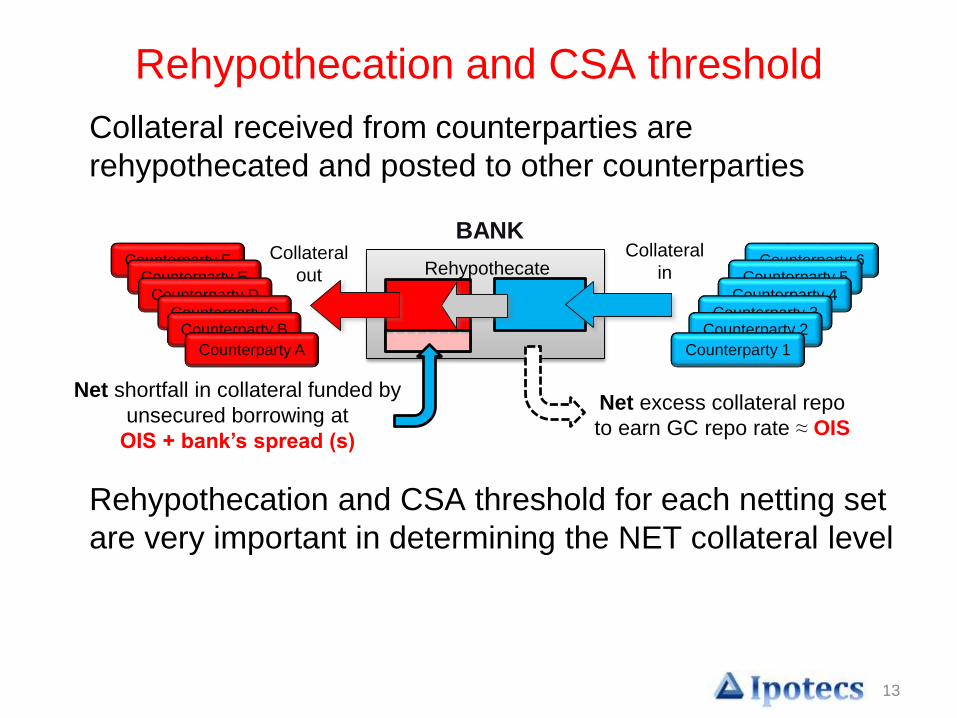
Rehypothecation and CSA threshold
Collateral received from counterparties are
rehypothecated and posted to other counterparties
Rehypothecation and CSA threshold for each netting set
are very important in determining the NET collateral level
Counterparty 6Counterparty 5
Counterparty 4Counterparty 3
Counterparty 2
Counterparty 1
BANKCounterparty F
Counterparty ECounterparty D
Counterparty CCounterparty B
Counterparty A
Net excess collateral repo
to earn GC repo rate ≈ OIS
Net shortfall in collateral funded by
unsecured borrowing at
OIS + bank’s spread (s)
Collateral
inCollateral
out Rehypothecate
14
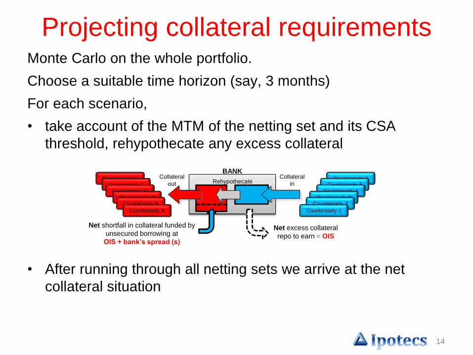
Monte Carlo on the whole portfolio.
Choose a suitable time horizon (say, 3 months)
For each scenario,
• take account of the MTM of the netting set and its CSA
threshold, rehypothecate any excess collateral
• After running through all netting sets we arrive at the net
collateral situation
Counterparty 6Counterparty 5
Counterparty 4
Counterparty 3Counterparty 2
Counterparty 1
BANKCounterparty F
Counterparty E
Counterparty D
Counterparty CCounterparty B
Counterparty A
Net excess collateral
repo to earn ≈ OIS
Net shortfall in collateral funded by
unsecured borrowing at
OIS + bank’s spread (s)
Collateral
in
Collateral
out Rehypothecate
Projecting collateral requirements
15
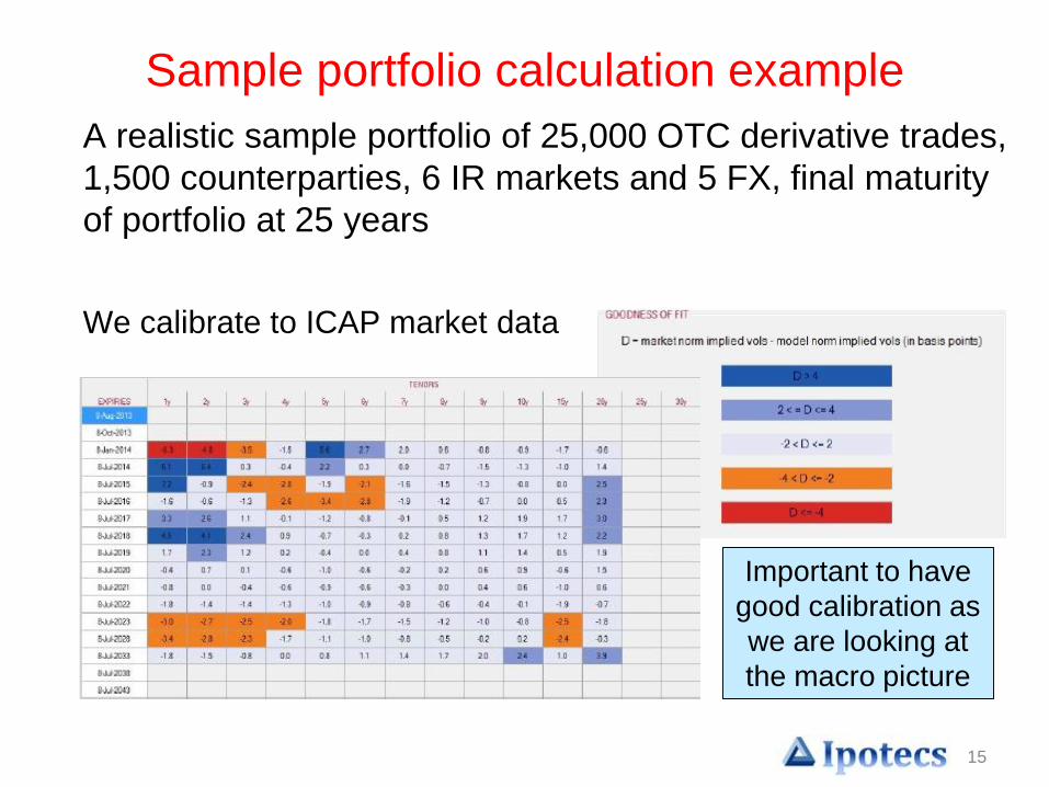
Sample portfolio calculation example
A realistic sample portfolio of 25,000 OTC derivative trades,
1,500 counterparties, 6 IR markets and 5 FX, final maturity
of portfolio at 25 years
We calibrate to ICAP market data
Important to have
good calibration as
we are looking at
the macro picture
16
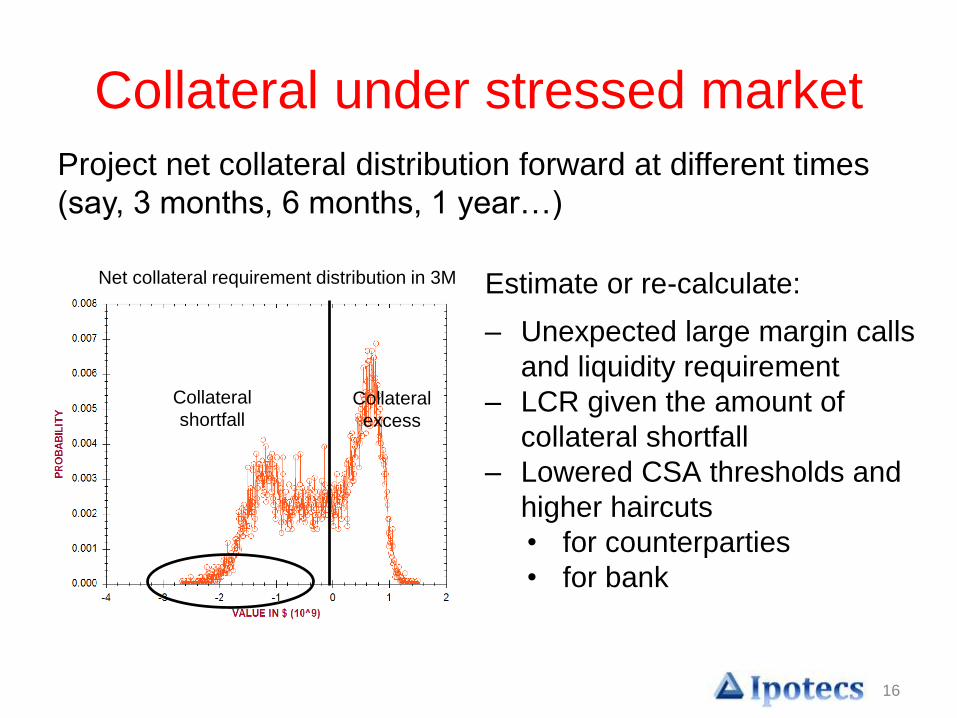
Collateral under stressed market
Estimate or re-calculate:
– Unexpected large margin calls
and liquidity requirement
– LCR given the amount of
collateral shortfall
– Lowered CSA thresholds and
higher haircuts
• for counterparties
• for bank
Project net collateral distribution forward at different times
(say, 3 months, 6 months, 1 year…)
Net collateral requirement distribution in 3M
Collateral
shortfallCollateral
excess
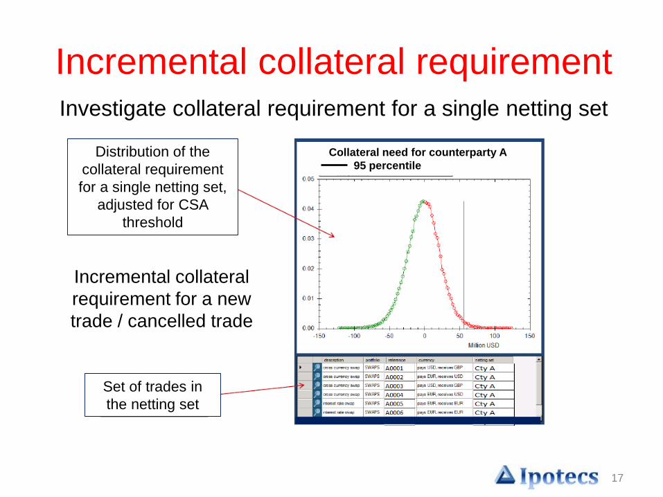
17
Distribution of the
collateral requirement
for a single netting set,
adjusted for CSA
threshold
Set of trades in
the netting set
Collateral need for counterparty A
95 percentile
Investigate collateral requirement for a single netting set
Incremental collateral requirement
Incremental collateral
requirement for a new
trade / cancelled trade
18
Modelling challenges
• It is very important to model re-hypothecation at the
portfolio level – not possible at transaction level or
even at netting set level
• One has to simulate all relevant market risk factors
but also credit qualities for all counterparties as CSA
agreement have credit dependencies
• Dynamic credit modelling is important also to model
the impact of defaults and gap risk on funding
requirements, and Wrong Way Risk (WWR)
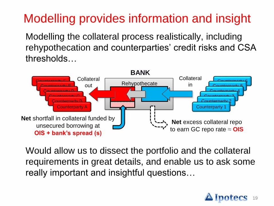
19
Modelling provides information and insight
Modelling the collateral process realistically, including
rehypothecation and counterparties’ credit risks and CSA
thresholds…
Would allow us to dissect the portfolio and the collateral
requirements in great details, and enable us to ask some
really important and insightful questions…
Counterparty 6Counterparty 5
Counterparty 4Counterparty 3
Counterparty 2
Counterparty 1
BANKCounterparty F
Counterparty ECounterparty D
Counterparty CCounterparty B
Counterparty A
Net excess collateral repo
to earn GC repo rate ≈ OIS
Net shortfall in collateral funded by
unsecured borrowing at
OIS + bank’s spread (s)
Collateral
inCollateral
out Rehypothecate
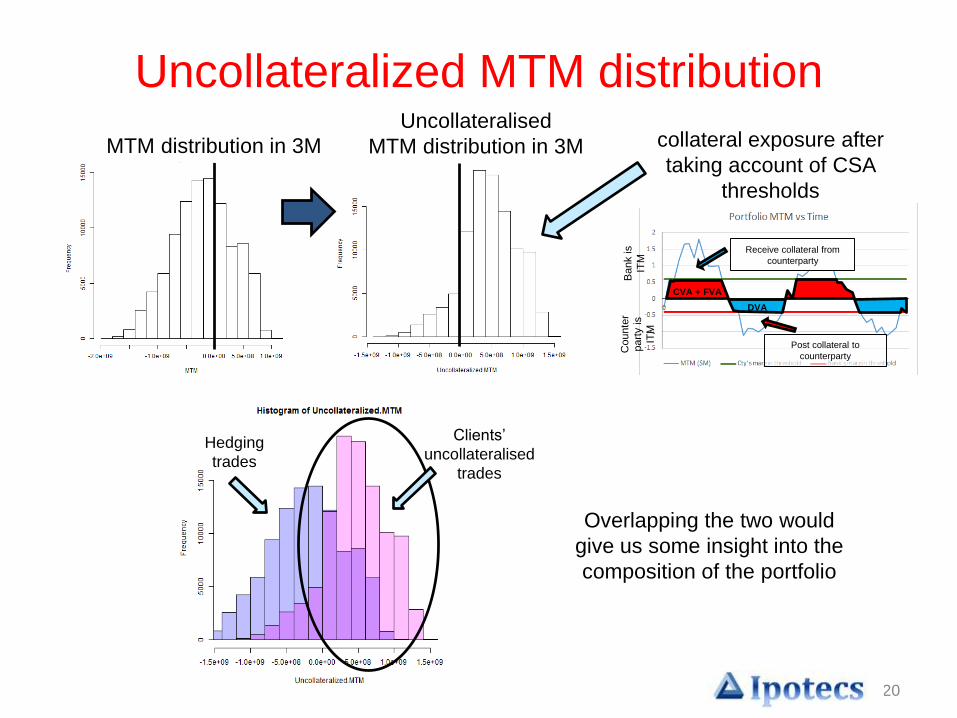
20
Uncollateralized MTM distribution
MTM distribution in 3M
Uncollateralised
MTM distribution in 3M
Bank is
ITM
Counte
r
part
y is
ITM
DVA
Receive collateral from
counterparty
CVA + FVA
Post collateral to
counterparty
collateral exposure after
taking account of CSA
thresholds
Clients’
uncollateralised
trades
Hedging
trades
Overlapping the two would
give us some insight into the
composition of the portfolio
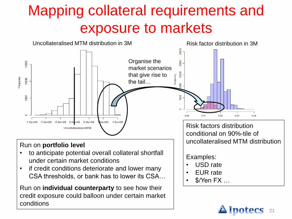
21
Risk factor distribution in 3M
Run on portfolio level
• to anticipate potential overall collateral shortfall
under certain market conditions
• if credit conditions deteriorate and lower many
CSA thresholds, or bank has to lower its CSA…
Run on individual counterparty to see how their
credit exposure could balloon under certain market
conditions
Uncollateralised MTM distribution in 3M
Organise the
market scenarios
that give rise to
the tail…
Risk factors distribution
conditional on 90%-tile of
uncollateralised MTM distribution
Examples:
• USD rate
• EUR rate
• $/Yen FX …
Mapping collateral requirements and
exposure to markets
22
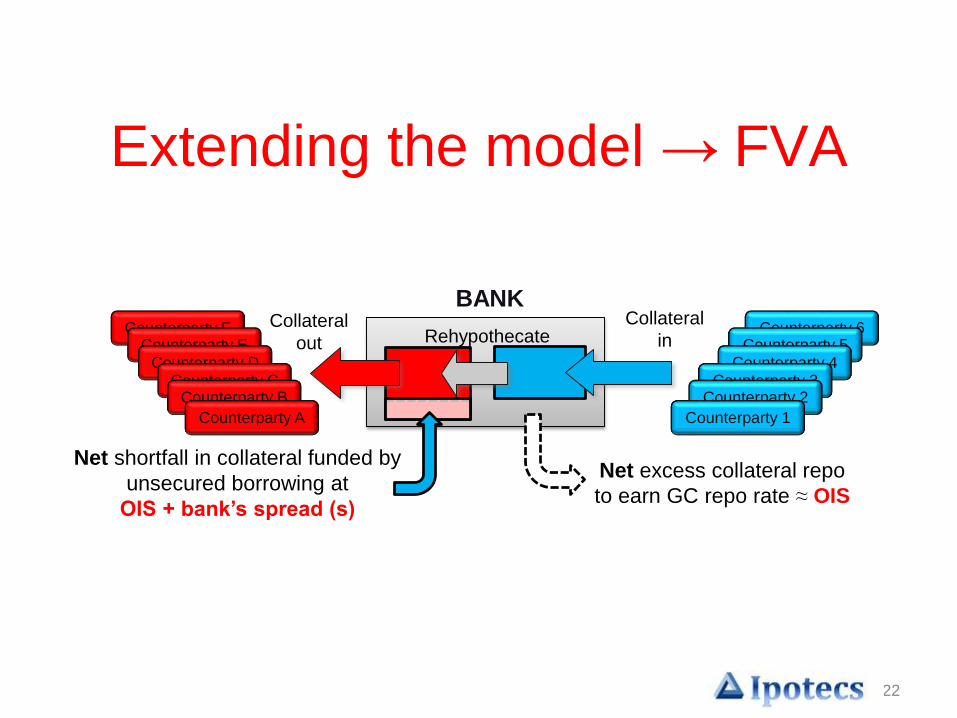
Extending the model → FVA
Counterparty 6Counterparty 5
Counterparty 4Counterparty 3
Counterparty 2
Counterparty 1
BANKCounterparty F
Counterparty ECounterparty D
Counterparty CCounterparty B
Counterparty A
Net excess collateral repo
to earn GC repo rate ≈ OIS
Net shortfall in collateral funded by
unsecured borrowing at
OIS + bank’s spread (s)
Collateral
inCollateral
out Rehypothecate
23
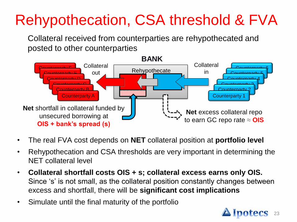
Rehypothecation, CSA threshold & FVA Collateral received from counterparties are rehypothecated and
posted to other counterparties
• The real FVA cost depends on NET collateral position at portfolio level
• Rehypothecation and CSA thresholds are very important in determining the
NET collateral level
• Collateral shortfall costs OIS + s; collateral excess earns only OIS.
Since ‘s’ is not small, as the collateral position constantly changes between
excess and shortfall, there will be significant cost implications
• Simulate until the final maturity of the portfolio
Counterparty 6Counterparty 5
Counterparty 4Counterparty 3
Counterparty 2
Counterparty 1
BANKCounterparty F
Counterparty ECounterparty D
Counterparty CCounterparty B
Counterparty A
Net excess collateral repo
to earn GC repo rate ≈ OIS
Net shortfall in collateral funded by
unsecured borrowing at
OIS + bank’s spread (s)
Collateral
inCollateral
out Rehypothecate
24
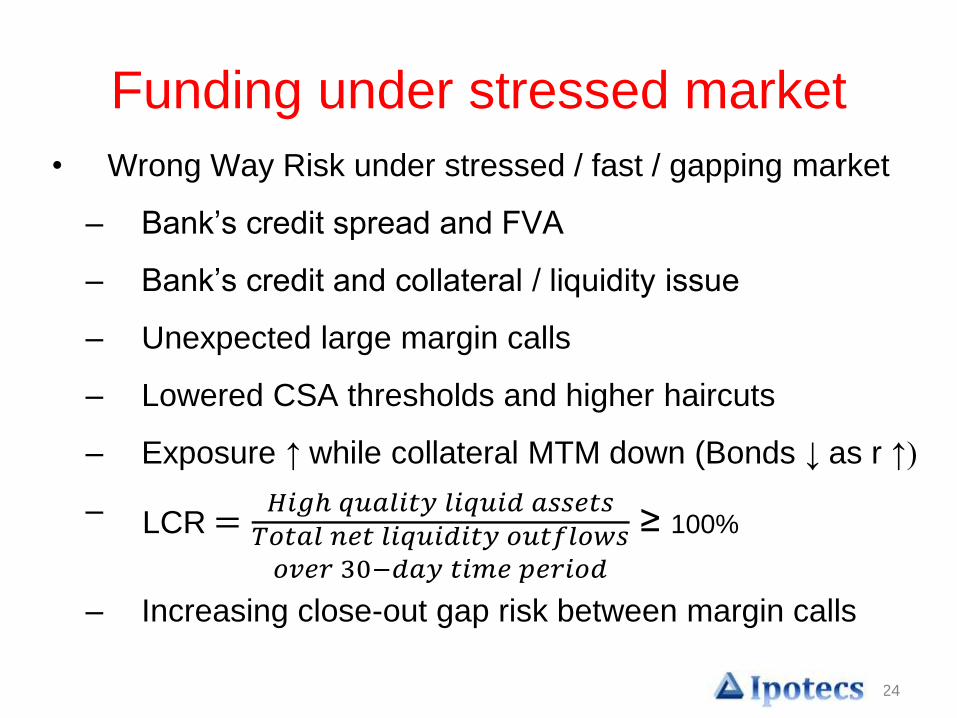
Funding under stressed market
• Wrong Way Risk under stressed / fast / gapping market
– Bank’s credit spread and FVA
– Bank’s credit and collateral / liquidity issue
– Unexpected large margin calls
– Lowered CSA thresholds and higher haircuts
– Exposure ↑ while collateral MTM down (Bonds ↓ as r ↑)
–
– Increasing close-out gap risk between margin calls
LCR=𝐻𝑖𝑔ℎ 𝑞𝑢𝑎𝑙𝑖𝑡𝑦 𝑙𝑖𝑞𝑢𝑖𝑑 𝑎𝑠𝑠𝑒𝑡𝑠𝑇𝑜𝑡𝑎𝑙 𝑛𝑒𝑡 𝑙𝑖𝑞𝑢𝑖𝑑𝑖𝑡𝑦 𝑜𝑢𝑡𝑓𝑙𝑜𝑤𝑠𝑜𝑣𝑒𝑟 30−𝑑𝑎𝑦 𝑡𝑖𝑚𝑒 𝑝𝑒𝑟𝑖𝑜𝑑
≥ 100%
25
FVA using funding rate discounting
Some FVA formulae in the literature use funding rate for
discounting.
Only a good approximation if borrowing rate = lending rate,
allowing costless netting of borrowing and lending cost in the
portfolio replication in the derivation.
=> FVA benefit will net against FVA cost with the same rate
That does not take into account the large cost difference
between unsecured borrowing rate (OIS + bank’s funding
spread) and the lending rate (repo at GC repo rate).
How much does it matter?
26
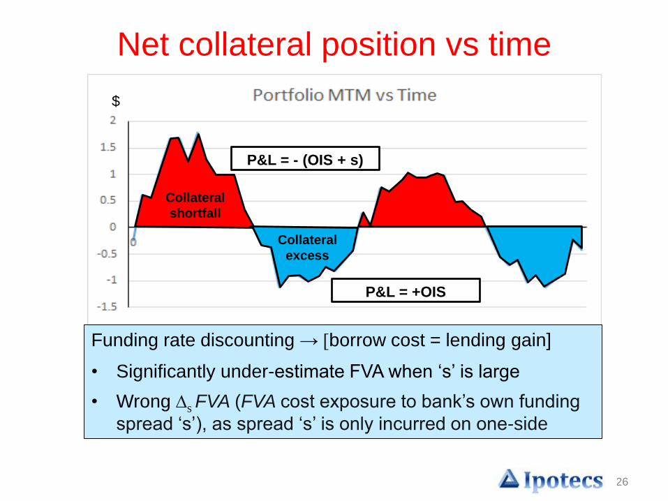
Net collateral position vs time
Collateral
shortfall
Collateral
excess
$
P&L = - (OIS + s)
P&L = +OIS
Funding rate discounting → [borrow cost = lending gain]
• Significantly under-estimate FVA when ‘s’ is large
• Wrong ∆s FVA (FVA cost exposure to bank’s own funding
spread ‘s’), as spread ‘s’ is only incurred on one-side
27
FVA using funding rate discounting
• Assuming the lending rate to equal the funding rate is an
approximation which is only correct in case there is never a
situation with excess collateral.
• One can use any excess collateral to buy back the bank’s
own debt, achieving lending gain = OIS + s (then sell them the
next day when requiring collateral). BUT…
• ALL excess collateral (from the portfolio) has to go towards
buying back the bank’s own debt. Repo-ing to get only GC
repo rate would incur a loss
Can this be achieved in practice?
If not, then the FVA, the risks and stress-testing
results, all could be significantly off…
28
Conceptual and accounting issues
• Non-unique asset exit prices – each bank has its own
funding cost
• Fair value includes discounting by unobservable
funding rate of the bank – under FASB 157, even
simple swap would needed to be classified as level 3
asset, consuming much more capital
• Double counting issues between DVA and FVA
• Partially collateralized transactions - ?
• Perverse incentive to encourage funding trades
(especially long-dated) with ‘phantom’ profit
• Hull and White: funding arbitrage trades
29
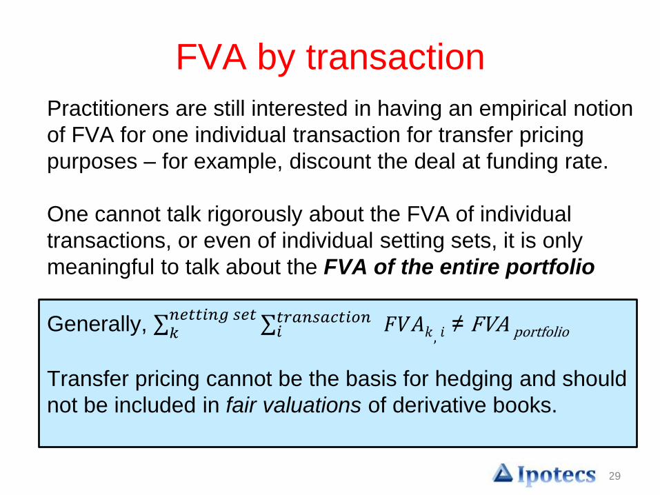
FVA by transaction
Practitioners are still interested in having an empirical notion
of FVA for one individual transaction for transfer pricing
purposes – for example, discount the deal at funding rate.
One cannot talk rigorously about the FVA of individual
transactions, or even of individual setting sets, it is only
meaningful to talk about the FVA of the entire portfolio
Generally, 𝑘𝑛𝑒𝑡𝑡𝑖𝑛𝑔 𝑠𝑒𝑡 𝑖
𝑡𝑟𝑎𝑛𝑠𝑎𝑐𝑡𝑖𝑜𝑛 𝐹𝑉𝐴𝑘, 𝑖 ≠ FVA portfolio
Transfer pricing cannot be the basis for hedging and should
not be included in fair valuations of derivative books.
Collateral
shortfall
Collateral
excess
Encourage long-dated funding trades
– earning OIS + s$
P&L = - (OIS + s)
P&L = +(OIS + s)
30
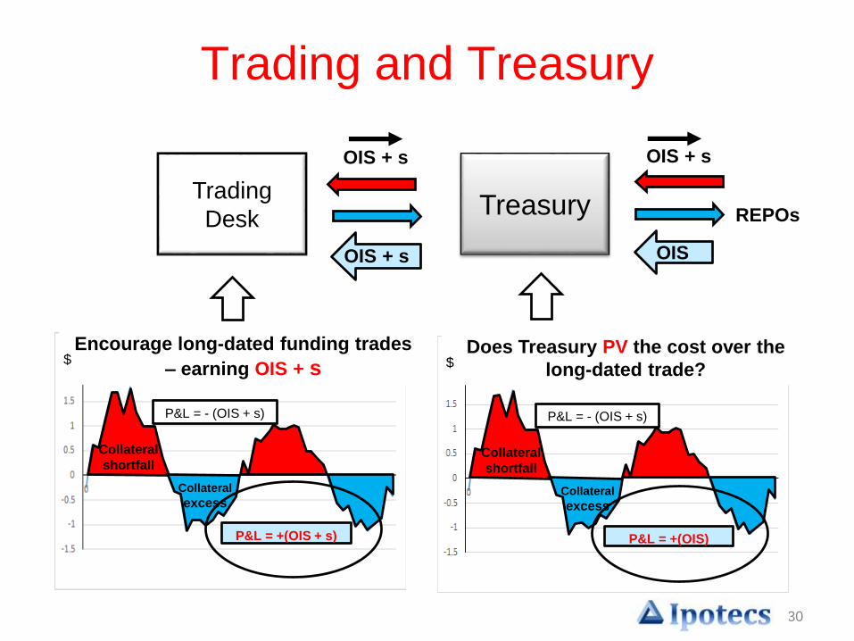
Trading and Treasury
Trading
DeskTreasury
OIS + s
OIS + s
OIS
OIS + s
Collateral
shortfall
Collateral
excess
Does Treasury PV the cost over the
long-dated trade?$
P&L = - (OIS + s)
P&L = +(OIS)
REPOs
31
Calculating FVA portfolio
The reality is that excess collateral gains OIS;
shortfall costs (OIS + s)
Discounting at funding rate does not capture all the
cost of FVA, gives wrong ∆s, and lead to
conceptual and accounting problems.
What is the alternative?
Suggestion:
• Model the process as it is at portfolio level,
and calculate the true FVA
32
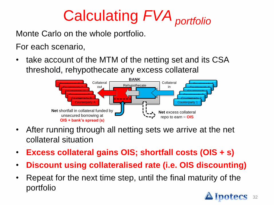
Monte Carlo on the whole portfolio.
For each scenario,
• take account of the MTM of the netting set and its CSA
threshold, rehypothecate any excess collateral
• After running through all netting sets we arrive at the net
collateral situation
• Excess collateral gains OIS; shortfall costs (OIS + s)
• Discount using collateralised rate (i.e. OIS discounting)
• Repeat for the next time step, until the final maturity of the
portfolio
Counterparty 6Counterparty 5
Counterparty 4
Counterparty 3Counterparty 2
Counterparty 1
BANKCounterparty F
Counterparty E
Counterparty D
Counterparty CCounterparty B
Counterparty A
Net excess collateral
repo to earn ≈ OIS
Net shortfall in collateral funded by
unsecured borrowing at
OIS + bank’s spread (s)
Collateral
in
Collateral
out Rehypothecate
Calculating FVA portfolio
33
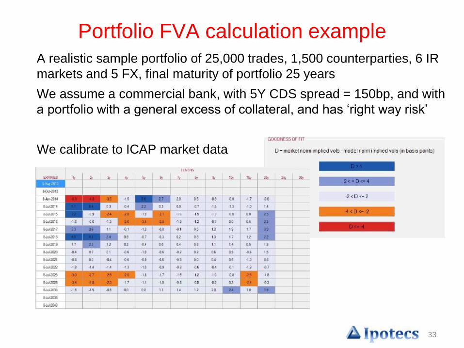
Portfolio FVA calculation example
A realistic sample portfolio of 25,000 trades, 1,500 counterparties, 6 IR
markets and 5 FX, final maturity of portfolio 25 years
We assume a commercial bank, with 5Y CDS spread = 150bp, and with
a portfolio with a general excess of collateral, and has ‘right way risk’
We calibrate to ICAP market data
34
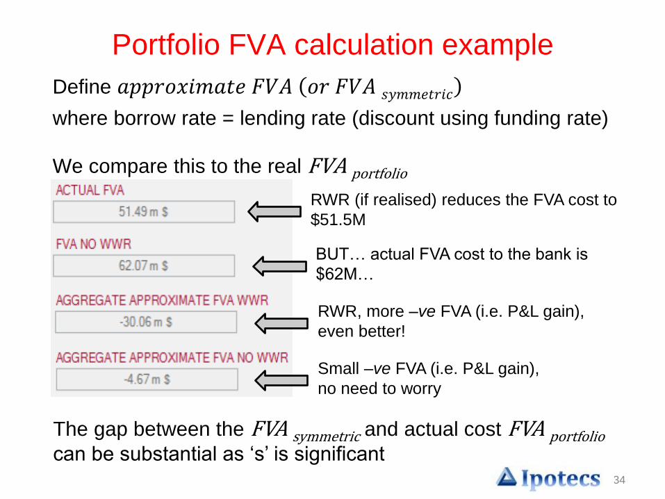
Portfolio FVA calculation example
Define 𝑎𝑝𝑝𝑟𝑜𝑥𝑖𝑚𝑎𝑡𝑒 𝐹𝑉𝐴 𝑜𝑟 𝐹𝑉𝐴 𝑠𝑦𝑚𝑚𝑒𝑡𝑟𝑖𝑐
where borrow rate = lending rate (discount using funding rate)
We compare this to the real FVA portfolio
Small –ve FVA (i.e. P&L gain),
no need to worry
RWR, more –ve FVA (i.e. P&L gain),
even better!
BUT… actual FVA cost to the bank is
$62M…
RWR (if realised) reduces the FVA cost to
$51.5M
The gap between the FVA symmetric and actual cost FVA portfoliocan be substantial as ‘s’ is significant
35
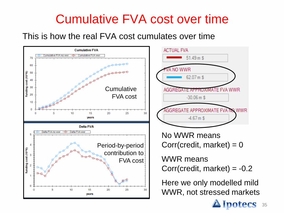
Cumulative FVA cost over time
This is how the real FVA cost cumulates over time
Period-by-period
contribution to
FVA cost
Cumulative
FVA cost
No WWR means
Corr(credit, market) = 0
WWR means
Corr(credit, market) = -0.2
Here we only modelled mild
WWR, not stressed markets
36
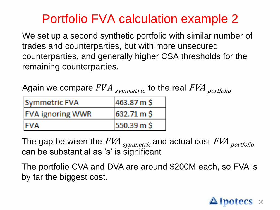
Portfolio FVA calculation example 2
We set up a second synthetic portfolio with similar number of
trades and counterparties, but with more unsecured
counterparties, and generally higher CSA thresholds for the
remaining counterparties.
Again we compare 𝐹𝑉𝐴 𝑠𝑦𝑚𝑚𝑒𝑡𝑟𝑖𝑐 to the real FVA portfolio
The gap between the FVA symmetric and actual cost FVA portfoliocan be substantial as ‘s’ is significant
The portfolio CVA and DVA are around $200M each, so FVA is
by far the biggest cost.
37
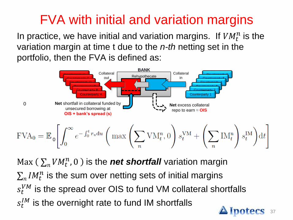
FVA with initial and variation margins In practice, we have initial and variation margins. If 𝑉𝑀𝑡
𝑛 is the
variation margin at time t due to the n-th netting set in the
portfolio, then the FVA is defined as:
Max 𝑛𝑉𝑀𝑡𝑛, 0 is the net shortfall variation margin
𝑛 𝐼𝑀𝑡𝑛 is the sum over netting sets of initial margins
𝑠𝑡𝑉𝑀 is the spread over OIS to fund VM collateral shortfalls
𝑠𝑡𝐼𝑀 is the overnight rate to fund IM shortfalls
Counterparty 6Counterparty 5
Counterparty 4
Counterparty 3Counterparty 2
Counterparty 1
BANKCounterparty F
Counterparty E
Counterparty D
Counterparty CCounterparty B
Counterparty A
Net excess collateral
repo to earn ≈ OIS
Net shortfall in collateral funded by
unsecured borrowing at
OIS + bank’s spread (s)
Collateral
in
Collateral
out Rehypothecate
0
0

38
Funding under stressed market
• Wrong Way Risk under stressed / fast / gapping market
– Bank’s credit spread and FVA
– Bank’s credit and collateral / liquidity issue
– Unexpected large margin calls
– Lowered CSA thresholds and higher haircuts
– Exposure ↑ while collateral MTM down (Bonds ↓ as r ↑)
–
– Increasing close-out gap risk between margin calls
LCR=𝐻𝑖𝑔ℎ 𝑞𝑢𝑎𝑙𝑖𝑡𝑦 𝑙𝑖𝑞𝑢𝑖𝑑 𝑎𝑠𝑠𝑒𝑡𝑠𝑇𝑜𝑡𝑎𝑙 𝑛𝑒𝑡 𝑙𝑖𝑞𝑢𝑖𝑑𝑖𝑡𝑦 𝑜𝑢𝑡𝑓𝑙𝑜𝑤𝑠𝑜𝑣𝑒𝑟 30−𝑑𝑎𝑦 𝑡𝑖𝑚𝑒 𝑝𝑒𝑟𝑖𝑜𝑑
≥ 100%
39
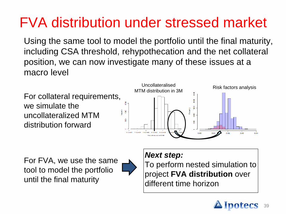
FVA distribution under stressed marketUsing the same tool to model the portfolio until the final maturity,
including CSA threshold, rehypothecation and the net collateral
position, we can now investigate many of these issues at a
macro level
Risk factors analysisUncollateralised
MTM distribution in 3M
For collateral requirements,
we simulate the
uncollateralized MTM
distribution forward
For FVA, we use the same
tool to model the portfolio
until the final maturity
Next step:
To perform nested simulation to
project FVA distribution over
different time horizon
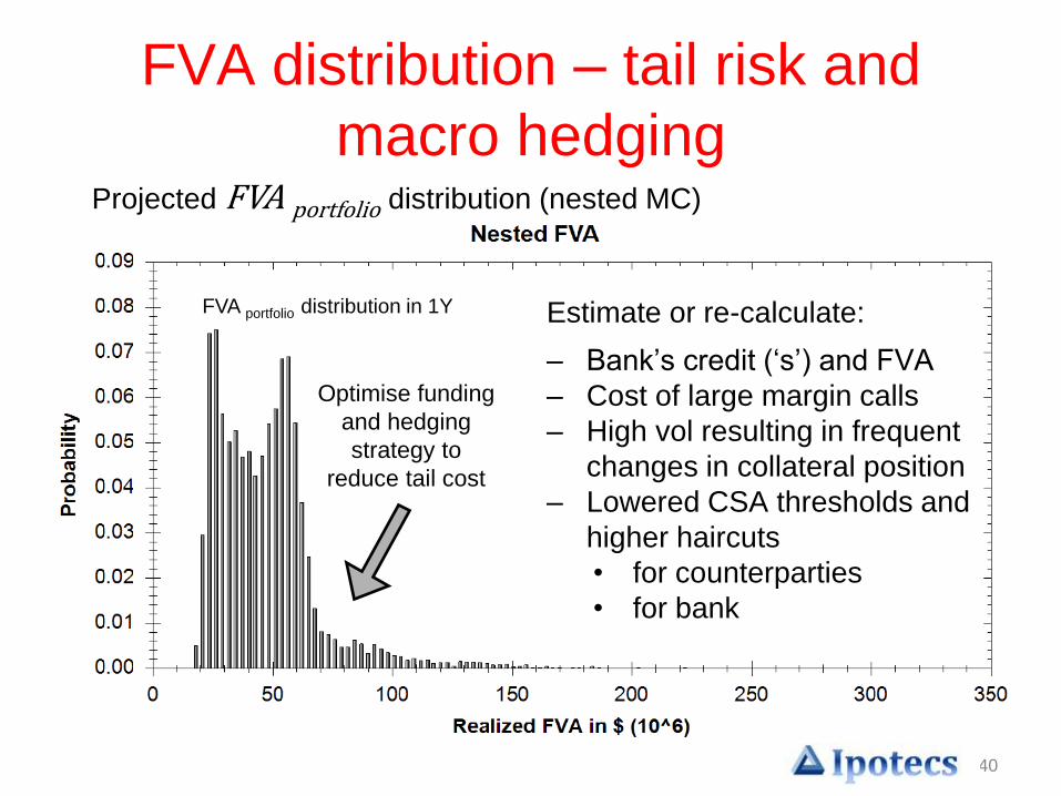
FVA portfolio distribution in 1Y
40
FVA distribution – tail risk and
macro hedging
Estimate or re-calculate:
– Bank’s credit (‘s’) and FVA
– Cost of large margin calls
– High vol resulting in frequent
changes in collateral position
– Lowered CSA thresholds and
higher haircuts
• for counterparties
• for bank
Projected FVA portfolio distribution (nested MC)
Optimise funding
and hedging
strategy to
reduce tail cost
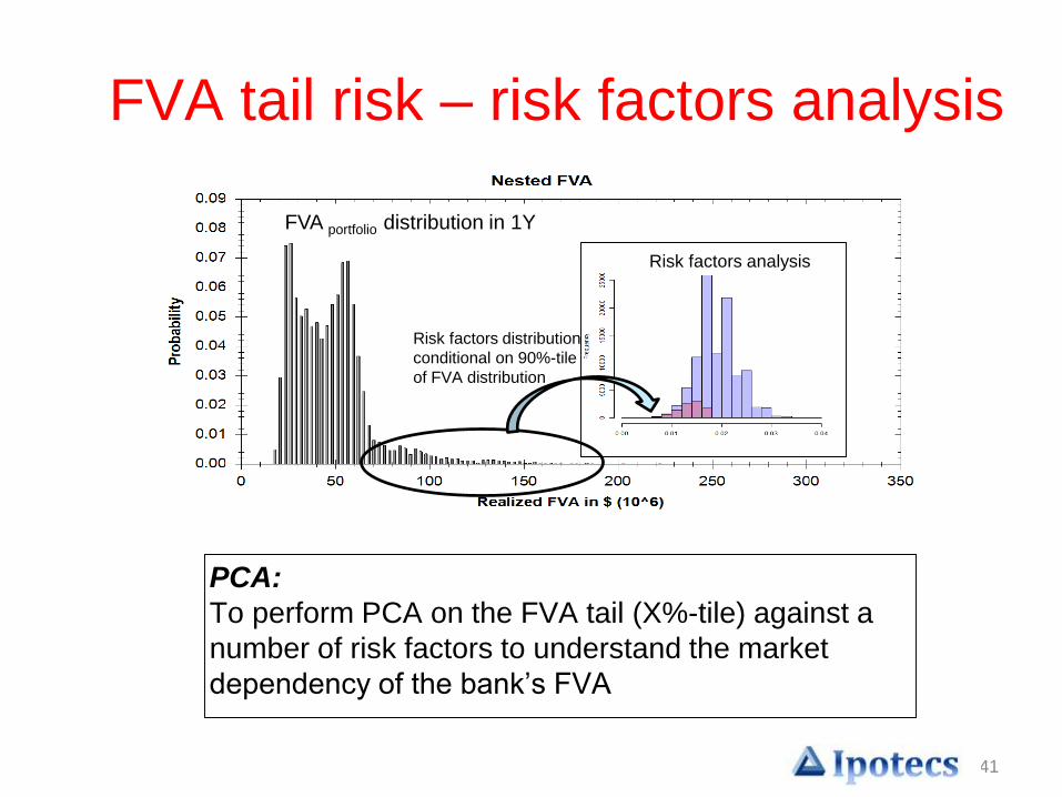
41
FVA tail risk – risk factors analysis
Risk factors analysis
FVA portfolio distribution in 1Y
PCA:
To perform PCA on the FVA tail (X%-tile) against a
number of risk factors to understand the market
dependency of the bank’s FVA
Risk factors distribution
conditional on 90%-tile
of FVA distribution
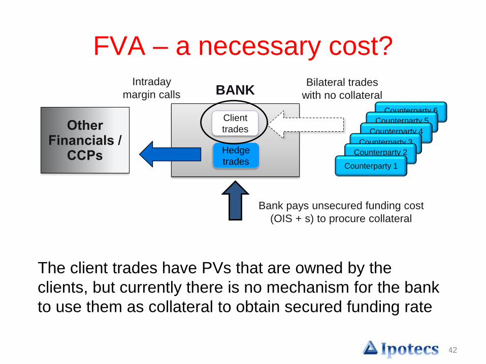
42
FVA – a necessary cost?
Counterparty 6
Counterparty 5
Counterparty 4
Counterparty 3
Counterparty 2
Counterparty 1
Other Financials /
CCPs
Bilateral trades
with no collateral
Client
trades
Hedge
trades
BANK
The client trades have PVs that are owned by the
clients, but currently there is no mechanism for the bank
to use them as collateral to obtain secured funding rate
Intraday
margin calls
Bank pays unsecured funding cost
(OIS + s) to procure collateral
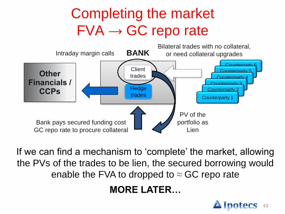
43
Completing the market
FVA → GC repo rate
Counterparty 6
Counterparty 5
Counterparty 4
Counterparty 3
Counterparty 2
Counterparty 1
Other Financials /
CCPs
Bilateral trades with no collateral,
or need collateral upgrades
Client
trades
Hedge
trades
BANK
If we can find a mechanism to ‘complete’ the market, allowing
the PVs of the trades to be lien, the secured borrowing would
enable the FVA to dropped to ≈ GC repo rate
MORE LATER…
Intraday margin calls
Bank pays secured funding cost
GC repo rate to procure collateral
PV of the
portfolio as
Lien
44
CVA under fast market
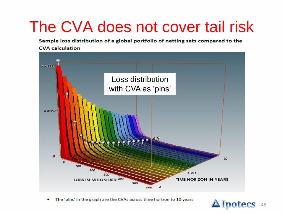
45
The CVA does not cover tail risk
Loss distribution
with CVA as ‘pins’
46
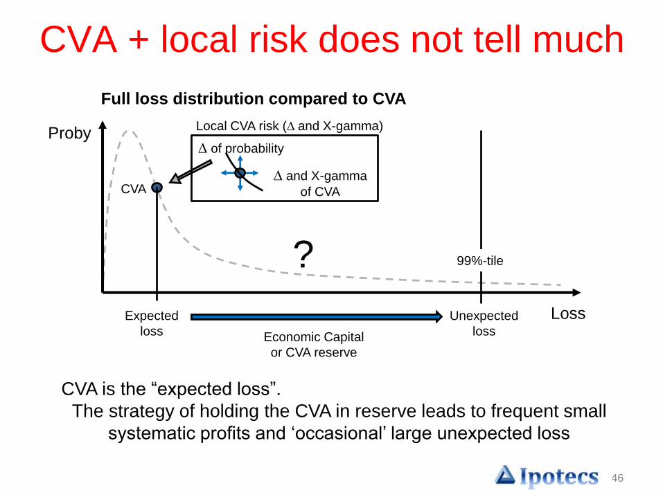
CVA + local risk does not tell much
CVA
Full loss distribution compared to CVA
Loss
Proby
99%-tile
Expected
loss
Unexpected
loss Economic Capital
or CVA reserve
Local CVA risk (∆ and X-gamma)
∆ of probability
∆ and X-gamma
of CVA
CVA is the “expected loss”.
The strategy of holding the CVA in reserve leads to frequent small
systematic profits and ‘occasional’ large unexpected loss
?
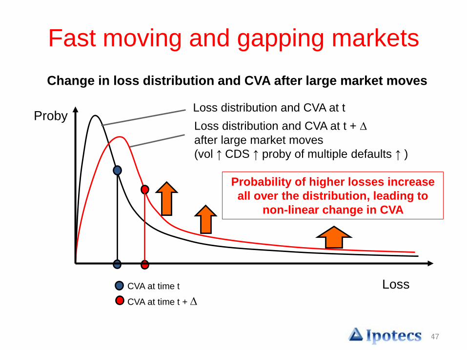
47
Loss
ProbyLoss distribution and CVA at t
Loss distribution and CVA at t + ∆
after large market moves
(vol ↑ CDS ↑ proby of multiple defaults ↑ )
Change in loss distribution and CVA after large market moves
Fast moving and gapping markets
CVA at time t
CVA at time t + ∆
Probability of higher losses increase
all over the distribution, leading to
non-linear change in CVA
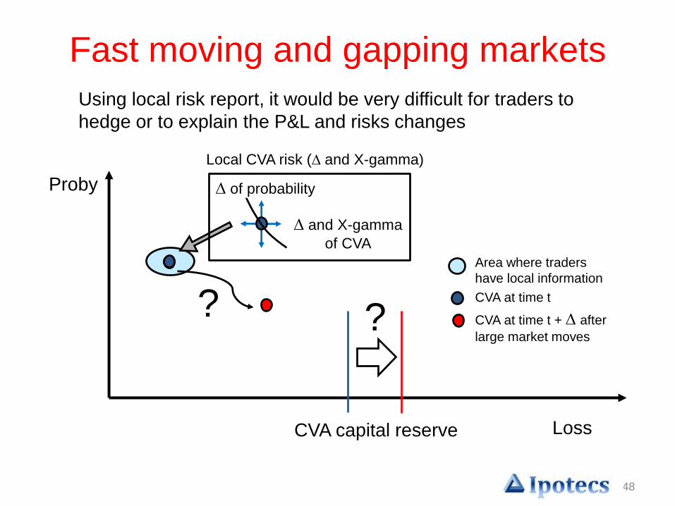
48
Using local risk report, it would be very difficult for traders to
hedge or to explain the P&L and risks changes
Loss
Proby
CVA capital reserve
Fast moving and gapping markets
? ?
Local CVA risk (∆ and X-gamma)
∆ of probability
∆ and X-gamma
of CVA
Area where traders
have local information
CVA at time t
CVA at time t + ∆ after
large market moves
49
Fast moving and gapping markets
CVA Risk
• Local delta, gamma + X-gamma cannot predict P&L
and risk for large moves
• Portfolio exposure and hedges could diverge rapidly
– fast expanding basis risk
• Wrong way risks become prominent
Potential large unexplained P&L and risk
Need global risk map and macro hedges
50
Fast moving and gapping marketsCVA Stress Test on its own inadequate to
control risk
• Too many risk factors, too many combinations – for
large market moves, large X-gammas, 3rd order, 4th
order – so many assumptions and combinations
• Can we afford to provision capital for ALL these
scenarios
• Can we decide on a good set of hedge trades among
these huge range of ‘artificial’ scenarios?
• Historical VaR – too few points to analyse the tail risk.
Future stress may come from different set of
scenarios. Can we find effective hedges based on
this analysis?
51
Fast moving and gapping markets
CVA Stress Test on its own inadequate to
control risk
• Wong way risks prominent
- Corr(Credit, Markets)
- Corr(Credit, Vol)
- Correlated defaults and downgrades
Stressed tests with static credit risk factors do
not give good estimates on the actual risk and
P&L
52
Collateral → FVA → CVA
With the tools we have developed, we now
investigate the ‘macro’ picture of the exposures
• Project loss distribution and investigate the
market scenarios contributing to different parts of
the loss distribution. Devise macro hedging
strategies, or simply reserve against the tail risk
(“unexpected loss”/economic capital)
• CVA distribution (the real CVA VaR) - perform
nested Monte Carlo simulation. Minimize the tail
through quasi-static or macro hedging
53
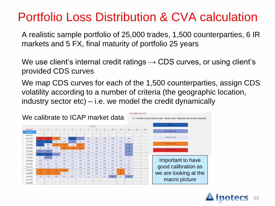
A realistic sample portfolio of 25,000 trades, 1,500 counterparties, 6 IR
markets and 5 FX, final maturity of portfolio 25 years
We use client’s internal credit ratings → CDS curves, or using client’s
provided CDS curves
We map CDS curves for each of the 1,500 counterparties, assign CDS
volatility according to a number of criteria (the geographic location,
industry sector etc) – i.e. we model the credit dynamically
Portfolio Loss Distribution & CVA calculation
Important to have
good calibration as
we are looking at the
macro picture
We calibrate to ICAP market data
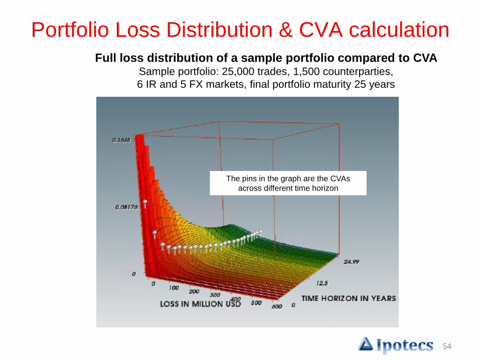
54
The pins in the graph are the CVAs
across different time horizon
Full loss distribution of a sample portfolio compared to CVASample portfolio: 25,000 trades, 1,500 counterparties,
6 IR and 5 FX markets, final portfolio maturity 25 years
Portfolio Loss Distribution & CVA calculation
CVA
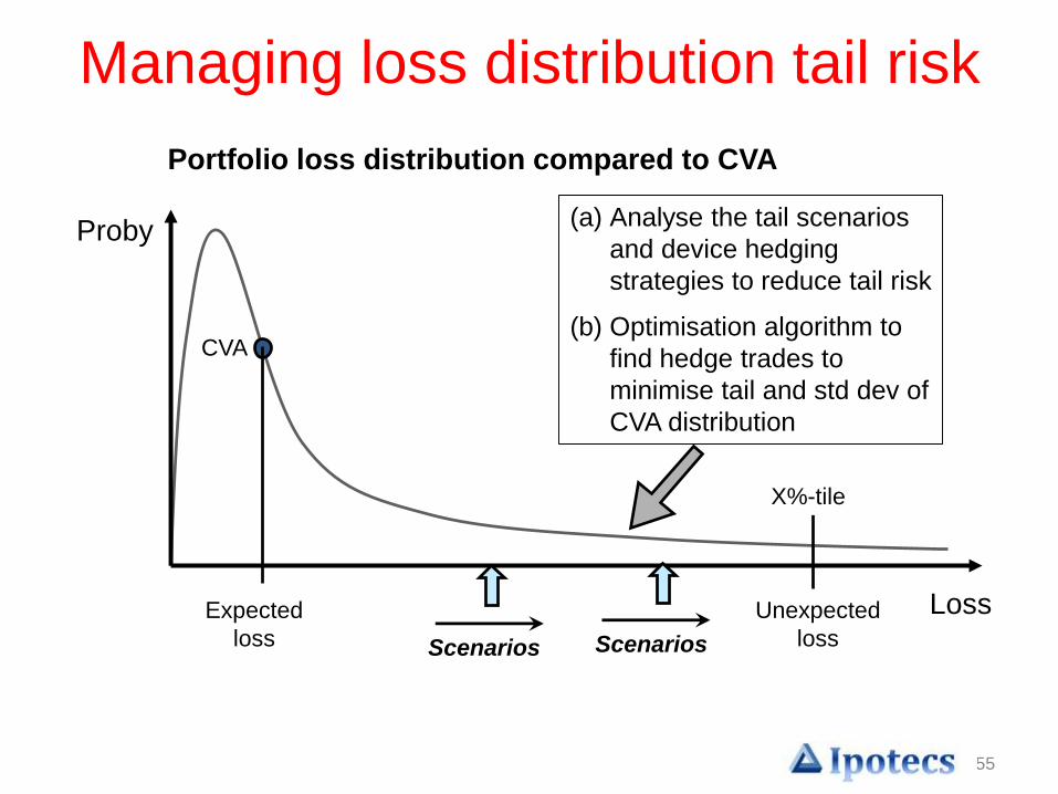
55
Managing loss distribution tail risk
Portfolio loss distribution compared to CVA
Loss
Proby
X%-tile
Expected
loss
Unexpected
loss
(a) Analyse the tail scenarios
and device hedging
strategies to reduce tail risk
(b) Optimisation algorithm to
find hedge trades to
minimise tail and std dev of
CVA distribution
Scenarios Scenarios
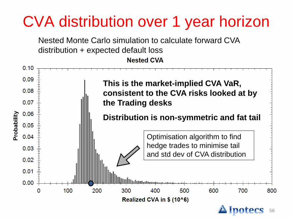
56
CVA distribution over 1 year horizon
Optimisation algorithm to find
hedge trades to minimise tail
and std dev of CVA distribution
Nested Monte Carlo simulation to calculate forward CVA
distribution + expected default loss
This is the market-implied CVA VaR,
consistent to the CVA risks looked at by
the Trading desks
Distribution is non-symmetric and fat tail
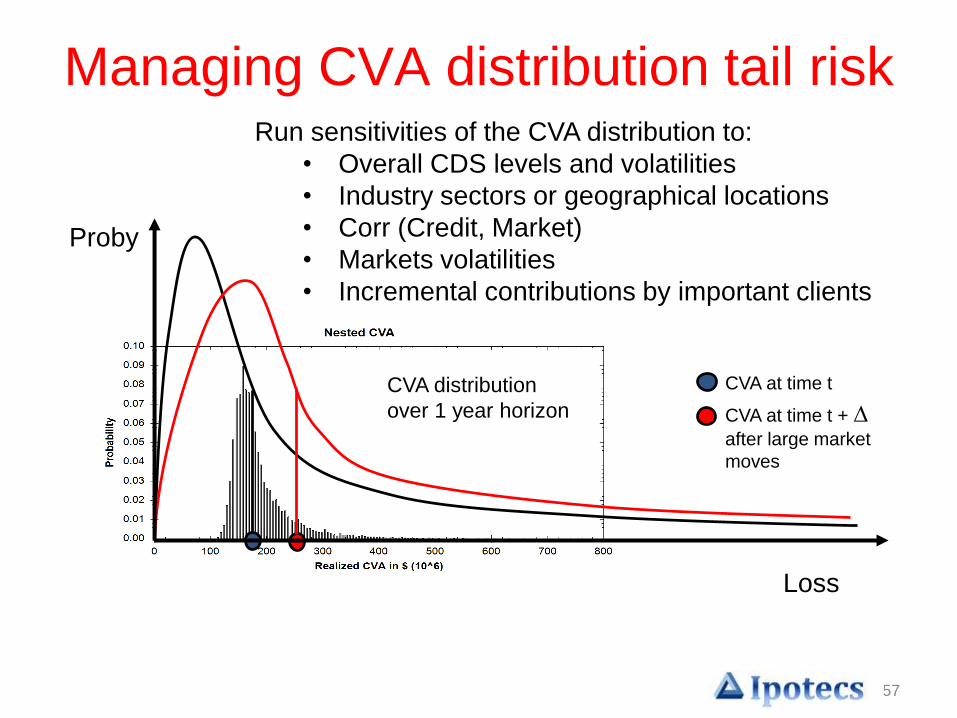
57
Loss
Proby
CVA distribution
over 1 year horizon
CVA at time t
CVA at time t + ∆after large market
moves
Run sensitivities of the CVA distribution to:
• Overall CDS levels and volatilities
• Industry sectors or geographical locations
• Corr (Credit, Market)
• Markets volatilities
• Incremental contributions by important clients
Managing CVA distribution tail risk
58
Static and dynamic CVA hedging
• Best risk management strategies combine
– Static hedging based on total return analysis over a
short time period (6m-1y)
– Dynamic hedging based on sensitivities
• Static hedging is useful because of the
gamma negative nature of the exposure
• Static hedging is useful because it dampens
the non-linear behaviour of the portfolio and
‘slows down’ the change in risks, enable
traders to manage through local hedgings

59
Combining Risk Management CVA, DVA and FVA

60
Collateral, CVA, DVA and FVAB
ank is IT
MC
ounte
rpart
y
is IT
M
DVA
Receive collateral from counterparty
CVA + FVA
Post collateral to counterparty
61
• The CVA, FVA and DVA change over time, are highly
correlated and could be more efficiently risk managed
together
• Important to have consistent modelling framework for
collateral, FVA, CVA and DVA, so risks can be
consistently aggregated and netted
• Best risk management strategies combine
– Static hedging based on total return analysis over a short
time period (6m-1y), to reduce the non-linearity of the risk
profile
– Dynamic hedging the ‘residual’ risks based on sensitivities
Combining CVA, DVA and FVA risks
62
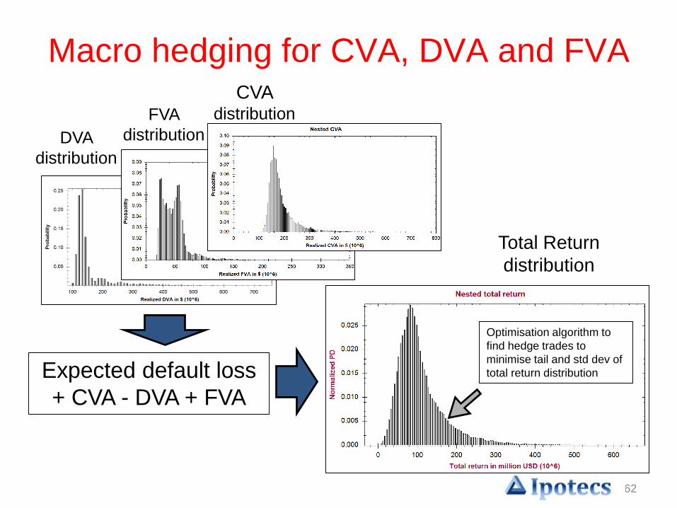
Macro hedging for CVA, DVA and FVA
Expected default loss
+ CVA - DVA + FVA
CVA distributionFVA
distributionDVA
distribution
Total Return
distribution
Optimisation algorithm to
find hedge trades to
minimise tail and std dev of
total return distribution
63
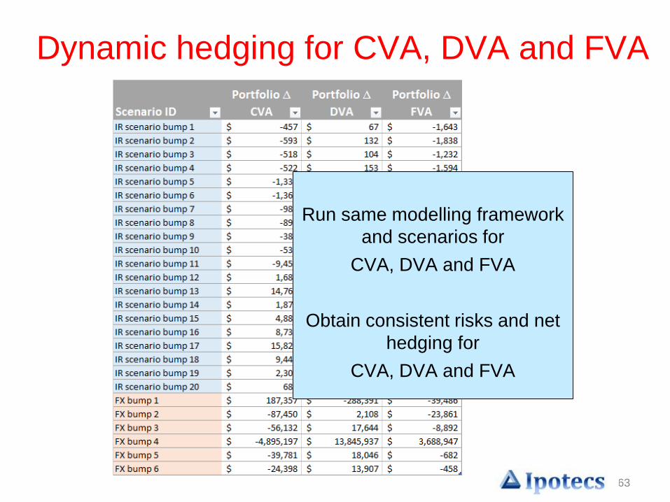
Dynamic hedging for CVA, DVA and FVA
Run same modelling framework
and scenarios for
CVA, DVA and FVA
Obtain consistent risks and net
hedging for
CVA, DVA and FVA
64
Sourcing collateral and
restructuring away the
FVA costs
65
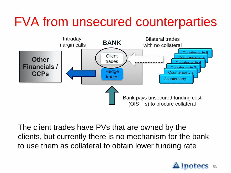
FVA from unsecured counterparties
Counterparty 6
Counterparty 5
Counterparty 4
Counterparty 3
Counterparty 2
Counterparty 1
Other Financials /
CCPs
Bilateral trades
with no collateral
Client
trades
Hedge
trades
BANK
The client trades have PVs that are owned by the
clients, but currently there is no mechanism for the bank
to use them as collateral to obtain lower funding rate
Intraday
margin calls
Bank pays unsecured funding cost
(OIS + s) to procure collateral
66
A mortgage analogy
• Consider a firm that wishes to buy real estate but there is no mortgage market
• Not being able to pass on a lien to the lender, the firm takes out an unsecured loan, at a high rate
• Upon defaulting, the firm still owns the title to the asset
• The liquidation process then redistributes wealth and losses among all creditors according to seniority
• The key difference between the two scenarios is that, while the mortgagor would have recovered the asset value in full, the unsecured lender may only recovers partially
• Hence, the fair value rates for unsecured lending normally exceed mortgage rates
67
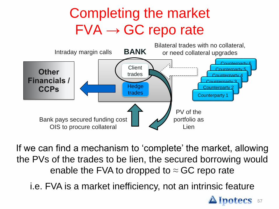
Completing the market
FVA → GC repo rate
Counterparty 6
Counterparty 5
Counterparty 4
Counterparty 3
Counterparty 2
Counterparty 1
Other Financials /
CCPs
Bilateral trades with no collateral,
or need collateral upgrades
Client
trades
Hedge
trades
BANK
If we can find a mechanism to ‘complete’ the market, allowing
the PVs of the trades to be lien, the secured borrowing would
enable the FVA to dropped to ≈ GC repo rate
i.e. FVA is a market inefficiency, not an intrinsic feature
Intraday margin calls
Bank pays secured funding cost
OIS to procure collateral
PV of the
portfolio as
Lien
68
Completing the market
FVA → GC repo rate
If we completing the market allowing the PVs of the trades to
be lien, the secured borrowing would enable the FVA to
dropped from bank’s funding spread ‘s’ to ≈ GC repo rate
Secured borrowing rate = lending rate = GC repo rate ≈ OIS
Now FVA benefit will net against FVA cost with the same rate
All assets can be discounted at the same rate at OIS.
Resolve a number of complicated issues:
• Unique price for the asset
• No FVA and no double counting DVA/FVA
• No perverted incentive to engage in funding trade for
‘phantom’ profit
69
Securitization
Banks attempt to securitize their OTC derivatives portfolio, with very
limited success. We examine the general features of such
securitization scheme:
o Long-dated (5Y+)
o By necessity need substitutions as portfolio evolves over term
(new deals, new counterparties to replace those dropping out,
matured and terminated trades, option expiry and exercised,
cancellations etc)
o For investors, the risks are difficult to quantify, and there is
information asymmetry and advantage (the bank determines the
portfolio contents)
o Potential exposure could balloon vs fixed coupon over term
o Liquidity risk – difficult to unload
o Regulatory charge for securitization
Completing the market
70
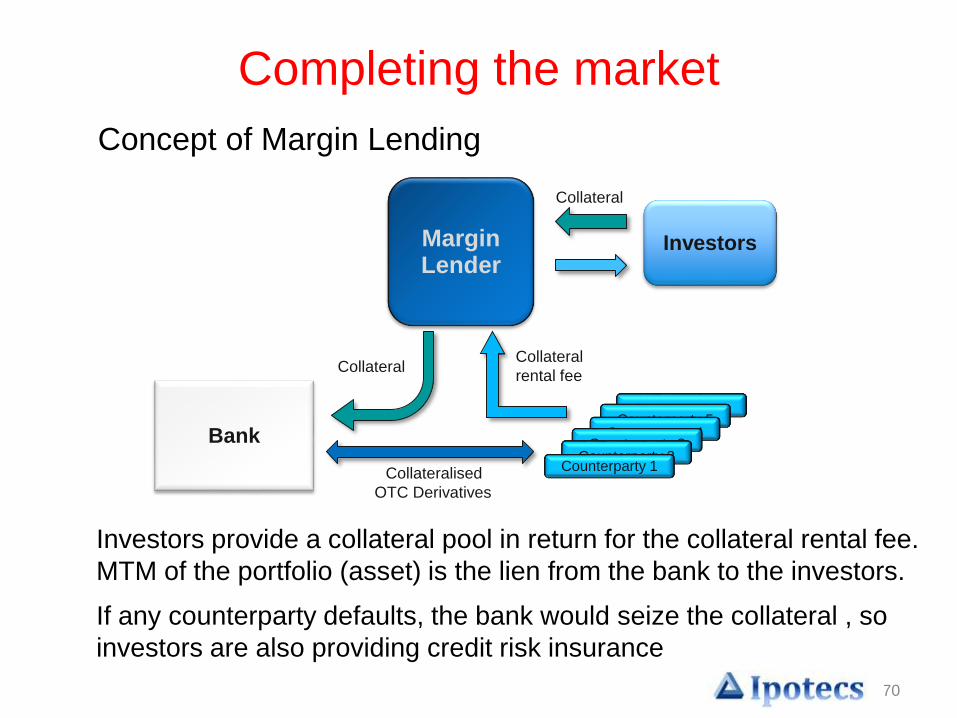
Completing the market
Investors provide a collateral pool in return for the collateral rental fee.
MTM of the portfolio (asset) is the lien from the bank to the investors.
If any counterparty defaults, the bank would seize the collateral , so
investors are also providing credit risk insurance
Margin Lender
Investors
Bank
Counterparty 6Counterparty 5
Counterparty 4Counterparty 3
Counterparty 2Counterparty 1
Collateral
rental fee
Collateralised
OTC Derivatives
Collateral
Collateral
Concept of Margin Lending
71
Benefit in completing the market
• Convert uncollateralised trades into fully collateralised trades, no
more FVA and its complications
• New sources of inexpensive eligible collaterals (secured borrowing
cost at GC repo rate ≈ OIS)
• Balance the collateral supplies and demands of the trading
portfolio, eliminating a lot of potential costs, and particularly
multitude of risks and exposures during stressed market conditions
• Add liquidity to the bank
• With fully collateralised trades, the bank can free up regulatory
capital in reduced CVA and CVA VaR charge
• Collateral providers are taking on the portfolio of a diversified
counterparties credit risk, not the credit risk of the bank. Hence
they are not limited by concentration credit risk to the bank
• Collateralising trades would free up unsecured client credit lines,
and would also make it easier to apply for new lines
72
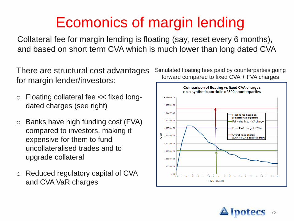
Ecomonics of margin lending
There are structural cost advantages
for margin lender/investors:
o Floating collateral fee << fixed long-
dated charges (see right)
o Banks have high funding cost (FVA)
compared to investors, making it
expensive for them to fund
uncollateralised trades and to
upgrade collateral
o Reduced regulatory capital of CVA
and CVA VaR charges
Collateral fee for margin lending is floating (say, reset every 6 months),
and based on short term CVA which is much lower than long dated CVA
Simulated floating fees paid by counterparties going
forward compared to fixed CVA + FVA charges
73
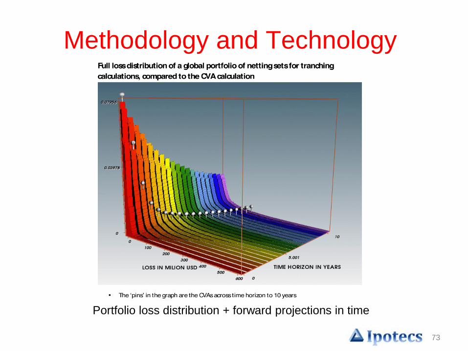
Methodology and Technology
Portfolio loss distribution + forward projections in time
74
Collateral / Margin Lending
• To procure these collateral, margin lender would
securitize the bank’s portfolio of counterparty credit risk
and perform maturity transformation
• To analyse margin lending portfolios one needs to
– Project out variation margin distributions
– Find cumulative loss distributions for the portfolio
– Find tranche loss distributions
• The analyses is based on the same technology
developed for loss distribution, CVA/DVA/FVA
distribution, and for collateral requirement projections
75
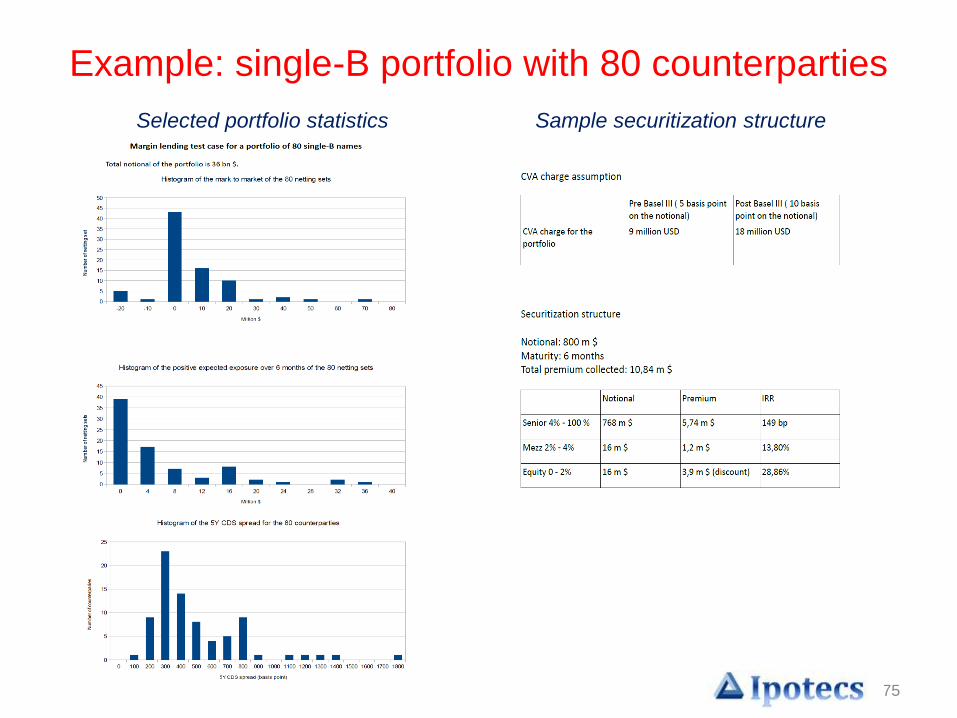
Example: single-B portfolio with 80 counterparties
Selected portfolio statistics Sample securitization structure
76
Collateral / Margin Lending

77
Contacts
Gary Wong
Prior to starting Ipotecs, he spent many years trading complex structured derivatives and developing risk
management techniques and infrastructure to control risks. His latest role was Managing Director and
Business Head of Structured Trading Group in Mitsubishi UFJ Securities International (MUSI), responsible
for the P&L and business development of all structured derivatives. He and his groups developed
sophisticated models and high-end technology as a platform for financial trading and risk reporting, and for
many years was the most profitable group in MUSI.
Prior to this, he was a trader and developed the exotic derivatives trading capability in Mizuho
International. Before that, he was in JP Morgan Asset Management, working on asset allocation models,
and IT infrastructure including real-time derivatives and options pricing system. He has both BSc (1st
class) and PhD in Physics from Imperial College, London University.
[email protected] Albanese
In 2006 he founded Global Valuation Limited (GVL), and introduced a novel approach to consistent
portfolio processing based on cutting edge computer engineering and an innovative mathematical
framework. He has been consulting on complex financial modelling issues and technology with a
number of top financial institutions including Morgan Stanley, Credit Suisse, Merrill Lynch/Bank of
America, Mitsubishi UFJ Securities, HSBC and Bloomberg amongst others.
He holds a PhD in Theoretical Physics from ETH Zurich and held professorships at the University of
Toronto and Imperial College London.

78
Contacts:
Claudio Albanese CEO
Gary Wong CEO
9 Devonshire Square
London EC2M 4YF