CUTTING FORCE MODELING AND OPTIMIZATION IN 3D

PLANE SURFACE MACHINING

Ning Su

Faculty of Engineering Science

Department of Mechanical & Materials Engineering

Submitted in partial fdfilment

of the requirements for the degree of

Master of Engineering Science

Faculty of Graduate Studies

The University of Western Ontario

London, Ontario

April, 1999

O Ning Su 1999

National Library I * m ofCanada Bibliothèque nationale

- du Canada

Acquisitions and Acquisitions et Bibliographie Services s e ~ k e s bibliographiques

395 Wellington Street 395. rue Wellington Ottawa ON K1A ON4 w w a ON K1A O N 4 Canada CaMda

The author has granted a non- L'auteur a accordé une licence non exclusive licence allowing the exclusive permettant à la National Library of Canada to Bibliothèque nationale du Canada de reproduce, loan, distribute or sell reproduire, prêter, distribuer ou copies of ths thesis in microfom, vendre des copies de cette thèse sous paper or electronic formats. la forme de microfiche/nlm, de

reproduction sur papier ou sur format électronique.

The author retains ownership of the L'auteur conserve la propriété du copyright in this thesis. Neither the droit d'auteur qui protège cette thèse. thesis nor substantial extracts fkom it Ni la thèse ni des extraits substantiels may be printed or otherwise de celle-ci ne doivent être imprimés reproduced without the author's ou -autrement reproduits sans son permission. autorisation.

ABSTRACT

The prediction and optimization of cutting forces in the finish rnachining of 3D

plane surface using ball-end milling are presented in this thesis. The cutting force model

is developed based on the mechanistic modeling approach. The objective is to accurately

model the cutting forces for non-horizontal and cross-feed cutter movements in 3D

finishing ball-end milling. Main features of the model include: (1) a robust cut geometry

identification method to establish the complicated engaged area on the cutter; ( 2 ) a

generalized algorithm to determine the undeformed chip thickness for each engaged

cutting edge element; and (3) a comprehensive empirical chip-force relationship to

characterize non-horizontal cutting mechanics. Experimental results have shown that the

present model gives excellent predictions of cutting forces in 3D ball-end milling.

Optimization of the cutting forces is used to determine both the tool path and the

maximum feedrate in 3D plane surface finish machining. An integrated process planning

method based on cutting force optimization for the concurrent optimization of t001 path

and feedrate for the finish machining of 3D plane surfaces using ball-end milling is

presented. This method is based on the evaluation of machining errors caused by cutting

forces and cutting system deflections. Optimum tool path and feedrate are established

when the machining process is carried out at the highest possible eficiency and the

resulting machining errors are maintained within the specified tolerance limits. The

integrated optimization method determines the optimum cutter feed direction that

corresponds to the optimum tool path and feedrate. Simulation results have indicated that

the optimum cutter feed direction is ofien not unique but falis within an optimum range in

3D plane surface finishing machining.

ACKNOWLEDGEMENTS

1 would like to take this opportunity to thank my supervisor, Professor Hsi-Yung

Feng, for his valuable guidance, encouragement. and assistance.

My sincere appreciation also goes to rny fellow graduate students who provided

me with valuable assistance and suggestions.

The financial support provided by the Natural Sciences and Engineering Research

Council of Canada is gratefùlly acknowledged.

Last but not the least, 1 would like to thank my parents, Changsheng Su and

Lianqing Qin, for their endless support and kind encouragement throughout my academic

career.

TABLE OF CONTENTS

CHAPTER 1 INTRODUCTION ........................................................ 1

1.1 Background and Motivation . . . . . . .. . .. . ... ... . - - - - - - - - - - -. .. . . . .. . -. - . - . . . . . 1

1 - r : --- .--- i .L ~ t i c ~ aiul c KCVICW - . - - . . - - . . . . . . . . . . . * - . . - . - - . - . . - -. . - . . . . . - . . - - . . . . . . . . . - . . . . . . . 3

1.2.1 Cutting Force Modeling ... . .. . . . . .. ... . . . . - . - - - . - - - - . .-. . . . . . . . . . .. . .. 4

1.2.3 Process Planning for 3D Surface Machining . . . . . . . . . . . . . . . . . . . . - -. 6

1-3 Research Scope and Objectives . . . . . . . . . . . . . . . . . . - - - - - - - -. . . . - -. . . - - - - - - - - - -. . - - - 10

1.4 Thesis Overview . . . . . . . . . .. . ... . . . .. . . . . . . . . . . .. . ... . . . . . . . . . . . . . .. . .. .. . . . . . . . . . -. . . 1 1

CEAPTER 2 CUTTING FORCE MODELING FOR 3D BALL-END

MKLING ................-..- * - - - - - - - - - - - * . * . - . * ...* * * * - - - . - - - - * . - - * * . * . - - . 12

2.1 Introduction . , . . . . . . . . . . . . . . . . . . - - - - * * - - . - - - . . - -. . . . . * . - - - -. - - - . - - . -. -. - - . . -. . - - - . . 12

2.2 Mode1 Formulation . . . . . . . . . . . - . . . . . . . - - - - - - - -. . . - . . . . - . . - - - - - - - - - . . . . . . . - - - - . . . 13

2.2.1 Cut Geometry . . . . . . . . . . . . . . . . . . . . . . . . . .. . . . . . . .. . . . . . .. . . . . . . . . . . . . . . . . . . I6

2.2.2 Undeformed Chip Thickness . . . . . . . . . . . . . . . . . . . . . .. . . . - . . . . . . . . . -. . . 28

2 - 2 3 Empirical C hip-Force Relationships . . . . . . . . . . . . . . . . . . . . . . . . . . . . . . . . . . 3 5

2.2.4 Cutting Force CalcuIation .............................................. 38

2.3 Determination of Empirical Mode1 Parameters ................................. 39

2.4 Mode1 Validation and Discussions ................................................ 42

CHAPTER 3 INTEGlRATED PROCESS PLANNING BASED ON

CUTTING FORCE O f TIIMIZATION ................................. 52

3.1 Introduction .......................................................................... 52

3 -2 Mathematicai Formulation ......................................................... 54

3 2 . 1 Feed Direction ............................................................ 54

3-22 Step Size ................................................................... 58

3.2.3 Feedrate ................................................................... 62

3 .2.4 Machining Time ......................................................... 65

3 -3 Simulation Results and Discussions ........................................... 68

CHAPTER 4 CONCLUSIONS .............................................................. 79

APPENDTX ....................................................................................... 82

A . Determination of Cutter Contact Point Po (Xo, Yo, &) .......................... 82

B . Step Size Determination .......... ..... ........................................... 84

C . Limit Lines for Cutting System Deflections ..................................... 85

REFERENCES .................................................................................. 86

VITA ............................................................................................... 91

LIST OF FIGURES

2.1 A flow chart showing the cutting force calculation procedure ....................... 15

2.2 The Cartesian coordinate system used for the ball-end mil1 ........................... 17

.. ..................................................................... 2.3 Definitions of and 4 18

2.4 Sectional views of two special cases of cut geometry in 3D ball-end milling ...... 21

2.5 Two forms of milling: (a) up milling and (b) down milling .......................... 22

2.6 Coordinate system transformation ....................................................... 24

2.7 Typical cut geometry in 3D ball-end milling .......................................... 29

............................................................... 2.8 Cutter runout configuration 30

2.9 Undeformed chip thickness calculation geornetry for 3D ball-end milling ......... 32

2.10 Cutting forces for \y = O". <b = . 15". s = -3.175 mm. f = 0.03 8 1 mrn/tooth.

and d=6.35 mm ............................................................................ 44

2.1 1 The effect of cutter runout for = 0". 4 = . 15". s = -3.175 mm.

........................... ................. f = 0.038lmm~tooth. and J = 6-35 mm .... .. 46

2.12 Cutting forces for = 30°. 4 = OO. s = -3.175 mm. f = 0.038 1 mm/tooth.

and J = 6.286 mm .......................................................................... 47

2.13 Cutting forces for \~r = 40°. 4 = 1 5 O . s = -3.175 mm. f = 0.038 1 mdtooth.

and d = 6.286 mm .......................................................................... 49

2.14 Cutting forces for y = 30". 4 = . 15" . s = -3.175 mm. f = 0.038 1 mdtooth.

and J= 6.286 mm .......................................................................... 50

3 . I Machining time calculation procedure .................................................. 55

3 . 2 Part coordinate system and cutter coordinate systern .................................. 57

.......................................................... 3 -3 Step size calculation procedure 60

.................................................. 3.4 Tool path length calculation approach 66

3.5 Variation of (a) step size and (b) total tool path length with a .................. ..... 70

3.6 Variation of (a) feed per tooth and (b) machining error with a ...................... 72

3.7 Trajectorïes of cutting system deflections at different a ............................. 74

............................................................ 3.8 Machining time at different a 76

3-9 Machining time of plane surfaces at difFerent inclinations ........................... 78

A . 1 Determination of cutter contact point in the cutter coordinate system ............. 82

A.2 Step size determination geornetry ....................................................... 84

LIST OF TABLES

2.1 Values of the coefficients fomulated in Eq . (2.3 1) for the two no-horizonta1

siot cuts ....................................................................................... 42

2.2 Detailed cutting conditions for mode1 verification test cuts ........................... 43

2.3 Comparison of average prediction errors ............................................. 51

CHAPTER 1

INTRODUCTION

1.1 Background and Motivation

In modem manufacturing, products with 3D surfaces such as dies and molds in

the automotive industry, and cornpressor and turbine blades in the aerospace industry, are

widely used. These complex-shaped premium products are typically manufactured by

Computer Numerical Control (CNC) machines using ball-end mills. Ball-end mills are

used because they are easy to position with respect to the part surfaces and generate

simple and short Numerical Control WC) - pro.grarns. - Traditionally the majority of these

machining operations have been carried out with expenence-based approaches. The

optimum cutting conditions such as feedrate, step size between adjacent tool paths, and

depth of cut are determined aRer extensive shop floor tests. Very often, overly

conservative cutting conditions are selected to ensure high quality of the machined

product. This [irnits the process eficiency and leads to higher product cost. As more

emphasis is placed on the quality of the products and the productivity of the machining

process, it is necessary for the process planner to select the optimum cutting conditions

on a rational and scientific base so as to reduce or eliminate the effort involved in the

traditional trial and error method. As a result, mathematical models that c m accurately

characterize the performance of the particular machining processes need to be developed.

The cutting force acting on the cutter is one of the most important physical output

variables that encapsulate important cutting action information. The charactensation of

cutting forces is important for research and development into the modeling, optimization,

monitoring, and control of milling processes. By virtue of their ease of measurement and

their physical relevance, cutting forces often provide a key element to the understanding

of the machining process. In 3D surface machining with ball-end mills cutting forces are

modelled since they directly affect the produa quality and the process eficiency. It is

important that the cutting forces be maintained close to the optimum values durhg the

machining processes. Excessive cutting forces cause large cutting system deflections and

result in low product quality, while small cuning forces oflen indicate low machining

efficiency. Therefore, reliable quantitative predictions of cutting forces and cutting force

optimization in machining operations are essential for selecting optimal machining

conditions and determining rnachined part geometrical errors.

Process eEciency and product quality are essential to the cornpetitiveness of

manufacturing industries. To make products within specified tolerance with the least time

and the lowest cost is the ultirnate goal of modem manufacturing. In the rnachining

industry, high quality and cost effective machining can be achieved by the optimization

of the machining process. Traditional experience-based process planning methods often

generate less than optimal machiriing plan and tend to be conservative in the selection of

cutting conditions. The conservative cutting conditions represent low machining

eficiency and do not guarantee quality in machining parts with complex geometry. Out-

of-tolerance rnachined products are not uncornmon in practice. As a result, it is very

important to develop a process optimization method that is based on scientific knowledge

of machining and is able to generate optimized plans to achieve highest machining

efficiency and to ensure product quality.

Determination of optimum tool path and feedrate has been the critical task in

process planning for 3D surface machining. Current practice determines tool path and

feedrate individually. Optimization of these two variables is accomplished sequentially

and independently. This sequential approach Iimits further optimization of the machining

process and causes the produa to be made at a higher cost. Tool path and feedrate are in

fact closely related with each other. Changes in either parameter result in changes of

cutting forces. Therefore, optimization of cutting forces results in optimization of these

two variables. With the developed cutting force model, a true integrated process planning

method which is based on cutting force optimization for the concurrent determination of

tool path and feedrate in 3D plane surface finishing machining with ball-end mills is

presented in this work- Cutter feed direction and step size define the milling tool path for

3 D surface machining. Both of these two parameters are optimized simultaneously with

feedrate based on the caiculation of cutting forces and the resulting machining errors.

1.2 Literature Review

Cutting force modeling and optimization in end milling have been receiving much

attention for the Iast two decades. Lots of research work has been done on modeling of

the milling processes. Various process models have been developed by different

researchers fiom different points of view. Most of these models dealt with cutting forces

in machining. Much work has also been camed out on devrloping practical process

planning methods for 3D surface machining. The following sections give a review of the

work done by other researchers in the past two decades.

1.2.1 Czrtting Force Modeling

Much work has been done in the past related to the modeling of the end rnilling

processes. Comprehensive reviews on cutting force modeling for the milling processes

have been presented (Smith and Tlusty, 1991; Ehmam et al., 1997). Cutting force

modeling for flat-end milling has been the focus of many studies. In a senes of work by

Kline, DeVor et al. (DeVor et al., 1980; Kline et al., 1982% b; Kline and DeVor, 1983), a

mechanistic cutting force model for the fiat-end milling process was developed and used

to study problems associated with cutter runout, surface error generation, and machining

process planning. Yellowley (1985) developed a force model which separated the cutting

forces on the cutting edges into rake and flank face contributions. The cutting forces in

these mcc!e!s ire cz!cï!.'ed v:itk m ,ss~mptinn sf r ccrnp!e!e!y mzchizing system

in the flat-end rnilling processes. The associated cutting system deflections had no

feedback effect on the calcuIation of the cutting forces.

The first documented work which considered the complex chip geometry as a

result of the cutting system deflection feedback was done by Sutherland and DeVor

(1986) for the flat-end rnilling systems. Bayoumi et al. (1994% b) presented and validated

an analytic mechanistic cutting force model for milling operations. Cutting forces are

calculated by integrating the pressure and the fiction Ioads acting on the cutter surfaces

represented by ruled surfaces. Budak et al. (1996) modelled the cutting forces using a

unified cutting mechanics approach which relied on an experimentally determined

orthogonal cutting data base. This method eliminated the need for the experirnental

calibration of each mi lling cutter geometry required in the mechanistic approach of

cutting force prediction. Zheng et al. (1998) developed an explicit analytical cutting force

model for flat-end milling in the cutter angle domain based on finite-series

representations. The model formulation in this work led to a solution of force as an

algebraic function of tool geometry, rnachining parameters, cutting configuration, and

workpiece material properties. Mekote and Endres (1998) studied the importance of size

effects on milling processes and presented a detailed mechanistic analysis that included

size effects for slot rnilling operations. Zheng and Liang (1997) identified cutter axis tilt

in flat end milling process via cutting force analysis. Al1 the models mentioned above

deal with cutting force prediction in flat-end milling processes. Cut geometry in flat-end

mil1 is relatively simple and remains constant in the machining process.

Due to the complexity of the ball-end milling process, models for the prediction

and Sim and Yang (1993) analyzed the cutting geometry of a special ball-end mil1 with

plane rake faces, and, with the orthogonal machining data obtained fiom end tuming

tests, the cutting forces were predicted for rigid and flexible cutters. Feng and Menq

(1994a, b) successfully employed the mechanistic approach to model the complicated

bail-end milling process. A rigid system model was developed in their work which is

applicable to rigid ball-end miiling cutters with small tength-to-diameter ratios. Common

bal 1-end mi 11 ing cutters are, however, flexible and characterised with large length-to-

diameter ratios. A flexible system model was developed to consider this important

property of the cutting system (Feng and Menq, 1996). Yucesan and Altintas (1996)

analyzed the balt-shaped helical geometry of the cutting edges on the ball-end mill. The

cutting forces were calculated based on the pressure and the fiction load on the rake and

the clearance suI-faces of the cutting edges. The pressure and fiction coefficients are

identified from a set of slot bal1 end milling tests at different feeds and axial depth of

cuts, and were used to predict the cutting forces for various cutting conditions. More

recently, Abrari and Elbestawi (1997) presented and verified a closed form formulation

of cutting forces for both bal1 and flat end milling. The cutting forces were calculated

using the linear combination of a set of force basis hnctions.

It should be noted that most of the studies described above dealt with relatively

simple cut geometry and horizontal cutter movements. Though some claimed to be able

to model cutting forces for 3D end milling, no experimental validation was given.

Predicted cutting forces were only verified with simple horizontal cuts. The present work

is aimed at modeling the cutting forces for 3D ball-end milling. The previous work by

Fenz C- 2nd Menq (!496) v.+! he eeenderl te cc~s iAer the cîz.-!p!exities rz-sec! - I non- ---- horizontal and cross-feed movements of the ball-end mil1 in the finishing machining of

3D surfaces.

Many previous studies examined the geometnc aspects of milling tool path

generation in the machining of 3D surfaces. Since the late 1980's there has been an

enormous amount of work published on tool path generation from different points of

view. Much work was focused on part geornetry-related tool path generation in which the

major concems were the minimization of total tool path length and step size

maximization. Dragomatz and Mann (1997) gave a review on the development of NC

milling tool path generation since 1980s. Suh and Lee (1990) and Hwang (1992)

presented a method to determine the tool paths by calculating, at each path, the smallest

tool path interval (step size) and using it as a constant offset for the next tool path. The

reason for their selecting the srnaIlest interval as the offset distance is that this makes it

easy to define the constant isoparametnc offset as the next tool path, thereby satisming

the surface accuracy. However, one serious problem in this method is the un-controlled

scallop height left on the part surface, which causes either surface roughness (if too large)

or ineficient machining (if too small). A tool path planning method that kept the scallop

height constant was presented by Suresh and Yang (1994). Their work led to a reduction

of the cutter location (CL) data. Huang and Oliver (1992) descnbed a non-constant

parameter approach in tool path generation to solve the problem of eliminating

unnecessary cutter movement and gouging in sculptured surface machining. In their

approach step size is no longer constant and adjusted with the machined surface. A

computationally intensive approach to determine an accurate tme machining error was

used in their work. Lin and Koren (1996) developed a method based on non-constant

offset of the previous tool path to guarantee the cutter moving in an unmachined area of

the part surface and without redunrlant machining. In this method step size varied

according to the cutter radius and the local surface curvatures, and the scallop height was

maintained constant on the machined surface. To avoid excessive scallop height lefi on

sloped surfaces when constant step size is used, Marshall and Griffiths (1994) introduced

a tool path generation method in which extra milling occurs wherever it is needed; Le.,

when the surface is sloped. By this way the tool path and the resulting machining time are

dramatically reduced. Veeramani and Gau (1998) divided the machined surface into

small patches and minimized the machining tirne by arranging the sequence of their

machining order.

Besides total tool path length and step size, tool interference is another important

topic in tool path generation. Hwang (1992) developed an interference-free tool-path

generation method for 3D surface rnachining with ball-end mills. This work was Iater

extended to the machining of sculptured surface using flat and filleted endmills by

Hwang and Chang (1 998).

Many process planning methods that involve tool path planning and feedrate

optimization have also been developed. Dong et al. (1993) focused their work on tool

path and cutting condition optimization in sculptured surface rough machining. The tool

path is optimized by using a contour rnap cutting method to avoid an unnecessary cut.

The cutting condition parameters are optimized by taking into account both geometry-

optimization in the machining of 3D sculptured surface by studying the cut geometry of

the cutter. Boogert et al. (1996) considered the effect of cutting forces in their planning of

2'/2D tool paths for pnsmatic parts. Evan though cutting forces are taken into account in

their method, the method is mainly used to determine the cutting conditions for a pre-

selected tool path. The geometrical tool path calculation and cutting condition

determination are separated.

It should be noted that the optimization of tool path and cutting conditions in the

above studies was camed out independently and based on a sequential approach. It is

assumed that the optimal feed direction is already known or selected with experiences.

The optimal cutting conditions are then determined based on this preset feed direction.

Process planning in these methods is a sequential procedure. In addition, because the

cutting system is assumed to be completely rigid, cutting system deflection induced by

cutting forces is ignored. The geometry of the rnachined part is considered as the

determining factor in tool path generation. In fact, cutting forces should also be

considered since they cause inevitable cutting system deflection that often results in

signi ficant machining errors.

A recent work by Lim and Menq (1997) described a first attempt toward the

development of an integrated machining process planning method. This method

determined cutter feed direction and feedrate simuItaneousIy at discrete points on a part

surface. The step size of adjacent tool paths at these locations is assumed known and

independent of the optimization process. This preset step size resulted in varying scallop

height for different cutter feed direction in 3D surface machining. As a result, the milling

tool path is only partiallv - ootimized. The advantase of constant scallop height machining

to reduce redundancy and maximize efEciency was not considered.

For a particular 3D surface, the plane orientation relative to the cutter changes at

different cutter feed directions. This leads to different tool paths and cutting forces.

Among these different feed directions, only those that give maximum feedrate and

minimum machining errors are chosen as the practical machining directions. Cutting

forces at these directions are optimized. The complicated interactions among the feed

direction, the feedrate, the step size, the cutting forces, the resulting tool paths and

machining errors make it difficult to include al1 these factors in process planning. To

incorporate al1 these factors for optimal process planning is the main purpose of this

work. The true integrated process optimization is achieved when the machining process is

c-ed out at the highest possible feedrate and eficiency and the resulting machining

errors caused by cutting forces and cutting system deflections are maintained within the

specified tolerance limits.

1.3 Research Scope and Objectives

In the machining of a 3D surface, after the roughing cut, a semi-finish and finish

cut are required to bring the accuracy of the machined surface within stringent tolerance.

Since the surface dimensional errors are mainiy caused by the machining inaccuracies

associated with the finish pass, the present study is focused on the finishing milling

process analyses. In practice, the tool paths in machining 3D surfaces are approximated

by a series of line segments. It is then reasonable to approximate the 3D surface by a

series 3D plane surface patches. The present work is focused on cutting force prediction

and optimization for 3D plane surface machining. It represents an important step toward

the true optimization of the finish machining of sculptured surface using ball-end milis.

This thesis work consists of two main parts: cutting force modeling and process

planning based on cutting force optimization for 3D plane surface finish machining.

These two parts are closely reIated. The objective of this work in the first part is to

develop an accurate and practical cutting force model for ball-end milling in the finishing

machining of 3D plane surfaces. This requires the mode1 to be able to characterize the

cutting mechanics of non-horizontal and cross-feed cutter movements that are typical in

3D ball-end milling. The objective of the second part is to develop an integrated process

planning rnethod based on the developed ball-end milling cutting force model for the

three-axis finishing machining of 3D plane surfaces. The integrated process planning

process is achieved by optimizing cutting forces.

1.4 Thesis Overview

This thesis is focused on cutting force modeling and process planning based on

cutting force optimization in 3D plane surface finishing machining with ball-end mills.

Four chapters are written to document this work.

Chapter 1 provides the background information and review of milling process

modeling and process planning in 3D surface machining.

Chapter 2 presents an improved mechanistic cutting force model for the ball-end

milling process. A new cut geometry determination algorithm based on boundary limits

has been developed to identify engaged cutting edge elements. A generalized method is

used to establish the undeformed chip thickness for each engaged cutting element by

considering the radial difference between tooth trajectories. An improved empirical chip-

force relationship is developed to deal with non-horizontal cutter movements. The

developed model is validated by experimental results.

An integrated method for process planning based on cutting force optimization for

the finishing machining of 3D plane surfaces is presented in Chapter 3. It considers both

the part geornetry and the cutting forces in process planning. It facilitates the

deteminâtion of the most economical process plan for machining product with high

quality. Simulation results are provided to demonstrate the feasibility of this new

approach.

Concluding rernarks and future work recommendations are described in Chapter

4.

CHAPTER 2

CUTTING FORCE MBDELING FOR 3D BALL-END

MILLING

2.1 Introduction

Cutting forces are very important to the determination of rnachining errors in the

ball-end rnilling process. Machining errors of ball-end rnilled surfaces can be attributed to

a number of sources such as cutting system deflections, geometnc errors of the machine

tools, thermal effects of the machining processes, vibration, etc. Arnong them, the cutting

finishing ball-end milling. The cutting force, that is one of the output variables, is directly

influenced by any change taking place in rnachining. In ball-end milling, cutting forces

are generated by complicated interactions between the workpiece and the helical cutting

edges. The variables that affect cutting forces include feedrate, radial and axial depth of

cut, cutting speed, workpiece and cutting tool material, and cutting tool geometry.

The basic strategy to develop the present cutting force mode1 is to partition the

ball-end mil1 into a series of small disc-like elements along the cutter axis. The

undeformed chip geometry, which is central to the prediction of cutting forces, is

established by identiGing the cutting edge elements actively engaged in cutting for a

given cutter orientation and determining the undefomed chip thickness for each engaged

element. The elemental cutting force components for these elements are calculated fiom

the empirical chip-force relationships for the particular workpiece/cuîter combination.

The instantaneous cutting forces on the ball-end mil1 are then obtained by surnming the

contributions of al1 the erigaged cutting edge elements. The cutting system deflection is

taken as the immediate response of the cutting force; Le., the system inertia and the

cutting process damping are assumed to have no effect on the resulting deflection. The

compliance of the workpiece and the difference between the machine tool structure

compliance in different directions are assumed negligible. S ince end milling processes

are prone to the condition of chatter, the cutting conditions in the present work are

selected as suggested in the machining data handbooks such that the cutting operations

are smooth and no noticeable chatter is observed. The effects of chatter on the machining

process are therefore reduced to the least and not taken into account in the present model.

Accurate process models are essential to achieve optimum machining operations.

Typically, there are three kinds of machining process modeling approaches: analytical,

experimental, and mechanistic. It is easy to distinguish these models as their names

irnply. In analytical models, mathematical methods are employed to analyze the

machining processes and explicit analytical equations are derived. The advantage of

using analytical models is that it is more accurate. Nonetheless, as the machining system

becomes very complicated, difficulties arise in deriving explicit equations for this

complicated system. In experimenta! models, a lot of experiments need to be performed

to determine the empirical parameters and empirical expressions for the machining

system are obtained based on the empirical parameters. The dificulty of deriving

complicated mathematical expressions for the complicated machining systems is

eliminated when using experimental models. Yet, the large number of empirically

determined parameters makes the expressions of a machining system cumbersome and

impractical for many applications. The mechanistic approxh is a recent development. It

is rooted in both the analytical and the empirical modeling approaches and employs

computer simulation techniques. It is important to note that generally a combination of

these methods is needed to obtain a working mode1 since existing knowIedge is

insuficient to a o r d the superiority of any particular approach over the others. The

present work on cutting force rnodeling for 3D ball-end milling is based on the

mechanistic modeling approach.

Figure 2.1 shows the cutting force determination procedure in 3D ball-end

milling. Components essential to the determination of cutting forces include: the cut

gecmcq., '1- - - -- J-L-- - A -L:- *L: -1----- Ce- n - - r n r . A r r .++;.rrr elamant and t h e LllC UllUCiULLliCU LIlltJ LLtiLhllt33 lui bubli b i r p 5 b u e u b L i r i 5 *ubr - a w a a i - a r c , r u a u car-

empirical chip-force relationships. The first hvo components form undeformed chip

geometry on the ball-end mill. It refers to the geometry of the material that is to be

removed by the cutter at the particular moment. The empirical chip-force relationships

relate the cutting forces to the undeformed chip geometry. In a flexible cutting system,

system deflections caused by cutting forces redistribute the undeformed chip thickness

for each engaged cutting element. This effect is shown in the figure as a feedback from

the cutting forces to the undeformed chip thickness. The complexity and the methods to

establish these components for 3D ball-end milling will be discussed in detail in the

following sections.

1 1 1 1 1

Undefomed Chip 1 1

Cut Geometry

7

I Geometr y

Undeformed Chip - - Thickness 1

1 1

1 t

Empirical Chip-force Relationships i

I 1

I 1 1

Cutting Forces

Figure 2.1 A flow chart showing the cutting force calculation procedure.

Cut geometry is a very important parameter in the analysis of ball-end milling

mechanics. It represents the surface geometry generated by the cutter over one tooth

penod and also represents the engaged area on the cutter. Cut geometry is very

complicated in 3D ball-end milling due to the non-horizontal and cross-feed cutter

movements. A cutting edge element is considered engaged if it is within the cut

geometry. As the cutter rotates, a cutting edge element can be engaged constantly. or

become engaged and then disengaged, or be not engaged at all. Cut geometry is best

established using a comprehensive solid modeling approach. A preliminary generic solid

modeler based simulation system has recently been developed and demonstrated

av+iar;mfi~+oll.. Cr\- hm&yr\"+e.l Loll m:ll:r.rr /Cl h 8 o r . o r r . G n+ ol 1 CICIQ\ Cml:rl rnnJ~~l:*rr* W R p C . L L L I I + L l L U l l J L U 1 L L U l L L . U L L L U 1 V U l L - G L L U I I L L I I L I L ~ \Ll L V L V U L L U J L 1 b C Ut.. L //Li]. dV l lU L l l V U b b 4 4 I ~

techniques require large computing power for accurate simulations. A less computing

intensive but robust cut geometry identification method was developed in the present

work. This method utilizes boundary limits of the cutter-part engagement geometry to

establish the cut geometry and identify the engaged cutting elements for 3D ball-end

milling.

The compiex motion of the ball-end mil1 in the finish machining of 3D sculptured

surfaces results in cut geornetry that is continuously changing. Since the linear feed

movement of the cutter is often much smalIer than the rotational movement, cut geometry

at any cutter location can be approximated as if the cutter is machining a small 3D plane

surface patch. The small plane surface is tangent to both the bal1 surface of the cutter and

the 3D sculptured surface at the cutter contact point with the surface (surface generation

point of the cutter). Figure 2.2 shows the Cartesian coordinate system and the two

A-A sectioci: view (xz plane) B-B sectional view @z plane)

Figure 2.2 The Cartesian coordinate system used for the ball-end mill.

angular coordinates, y and 4, that are used to characterize the instantaneous cut

geornetry. The Cartesian coordinate system is established by setting (1) the tip at the free

end of the baii-end mil1 as the origin; (2) the cutter axis as the z axis; and (3) the plane

defined by the cutter feed direction and the cutter axis as the x z plane. The cross-section

of the bal1 part of the bail-end mil1 in the yz plane is a half circle. The angle is the

angle swept by the half circle until it reaches the surface generation point PO about an axis

that passes through (O,O,R) and is paralle1 to the y axis (R is the nominal radius of the

cutter). The angle d, is defined in a sirnilar way and by sweeping the half circle in the xz

plane about an axis parallel to the x axis. Definitions of y and 4 can also be seen in

Figure 2.2. It should be noted that the radii of the semi-circles in Figure 2.3 are generally

not equal to the nominal radius of the ball-end mill. The figure shows the cross-sections

of the cutter intersected by a plane parallel to wz plane and a plane parallel to yz piane

passing the surface generation points PO.

Figure 2.3 Definitions of y and 4.

Using the Cartesian coordinate system of the ball-end mill, the mathematical

equation for any point at the ball part of the cutter can be expressed as:

For the surface generation point Po (xo, yo, zo) on the ball part of the cutter, it c m be seen

f iom Figure 2.2 that

- xo - = tan \y R - zo

Substitution o f Eqs. (2.2) and (2.3) into Eq. (2.1) yields:

By substituting Eq. (2.4) into Eq. (2.2) and Eq. (2.3), the coordinate values of the surface

generaticn point Po can be obtained

- R t a n y xo =

JI + tan' + tan2$

Rtan+ Y0 =

JI i- tan' y + tan2$

According to the definition of y, when the cutter goes up in the feed direction, the value

of is negative. When the cutter goes down, the value of \y is positive.

Three geometric elements have been identified as the main factors that determine

cut geometry and control cutter engagement in 3D finishing ball-end milling: the part

surface preceding the current process (the semi-finished part surface), the dot surface lefi

by the adjacent finishing tool path, and the non-horizontal cutter feed direction. These

geometrïc elements define the boundary limits of the cutter-part engagement geometry.

Sectional views of two special cases of cut geometry in 3D ball-end rnilling are shown in

Figure 2.4: 4 = O (upper) and y = O (lower). In this figure, v is the non-horizontal

feedrate, f the feed per tooth, d the depth of cut, and s the step size.

There are two forms of milling to machine the workpiece: up milling and down

millinç, illustrated in Figure 2.5. In up milling, also called conventional milling, the

direction of motion of the cutter teeth is opposite to the feed direction of the workpiece

when the teeth cut into the work. It is milling "against the feed". In down milling, also

called climb milling, the motion direction of the cutter teeth is the same as the feed

direction of the workpiece when the teeth cut into the work. It is milling "with the feed"

(Groover, 1996). According to the definition of the coordinate system in the present

model, for up rnilling the step size is in the +y direction, while for down milling the step

size is in the -y direction.

It is evident from Figure 2.4 that the semi-finished part surface represents one of

the boundary limits. The semi-finished surface geometry is generated by the semi-

finishing process and can be complicated. It is simplified in the present work as an offset

Figure 2.4 Sectional views of two special cases of cut geometry in 3D ball-end milling.

Cuner rotation direction

\ - Feed direction \

Cutter rotation directrcn

( t Feed direction (

Figure 2.5 Two forms of rnilling: (a) up milling and (b) down milling (Groover, 1996).

suface to the finished surface with a uniform vertical offset d- This vertical offset is in

fact the axial depth of cut used in the current rnodel. The semi-finished part surface is

expressed in the cutter coordinate system as:

Let 2, donate the z coordinate value of any point on this surface. zP can be expressed as:

It is clear that cutting elements below this simplified surface can be engaged in cutting,

while cutting elements above this surface do not participate in cutting. This condition for

any cutting element at t can be given as follows:

If z 5 z , , the cutting element can be engaged in cutting;

If z > z, , the cutting element is not engaged in cutting.

The adjacent dot surface in finish ball-end milling represents another boundary

limit. In order to ensure the quality of the machined surface. the step size is usually very

small such that the scallop height is within the specified requirement. Due to the small

step size in the cross feed direction, part of the cutter falls inside the adjacent machined

slot (as shown in Figure 2.4) when the cutter is machining the current slot. Cutting

elernents within this adjacent rnachined slot are not engaged in cutting because the

materials within this area have been removed in the previous tool path. While cutting

elements outside this slot c m be participating in cuning. When the cutter moves non-

horizontally, the cross-section of the machined slot intersected by planes parallel to yz

piane becomes an eiiipse rather tnan a semi-circie. Eificuiries arise in cieternlltiirig iiiis

boundary limit when the current xyz coordinate system is used. It is noted that in the

pIane normal to the cutter feed direction, the cross-section of the dot is a semi-circle.

Therefore, to simpliQ the derivation, coordinate transformations are camied out to obtain

this boundary limit. The coordinate transformation procedure is illustrated in Figure 2.6.

The steps for the coordinate transformation are as follows:

1) Translation

Translation is made in the yr plane from the current coordinate system xyz to the

coordinate system dy'z' on the previous adjacent sIot surface. The new coordinates

(x ' ,~ ' , 2) in term of (x, y, z) are:

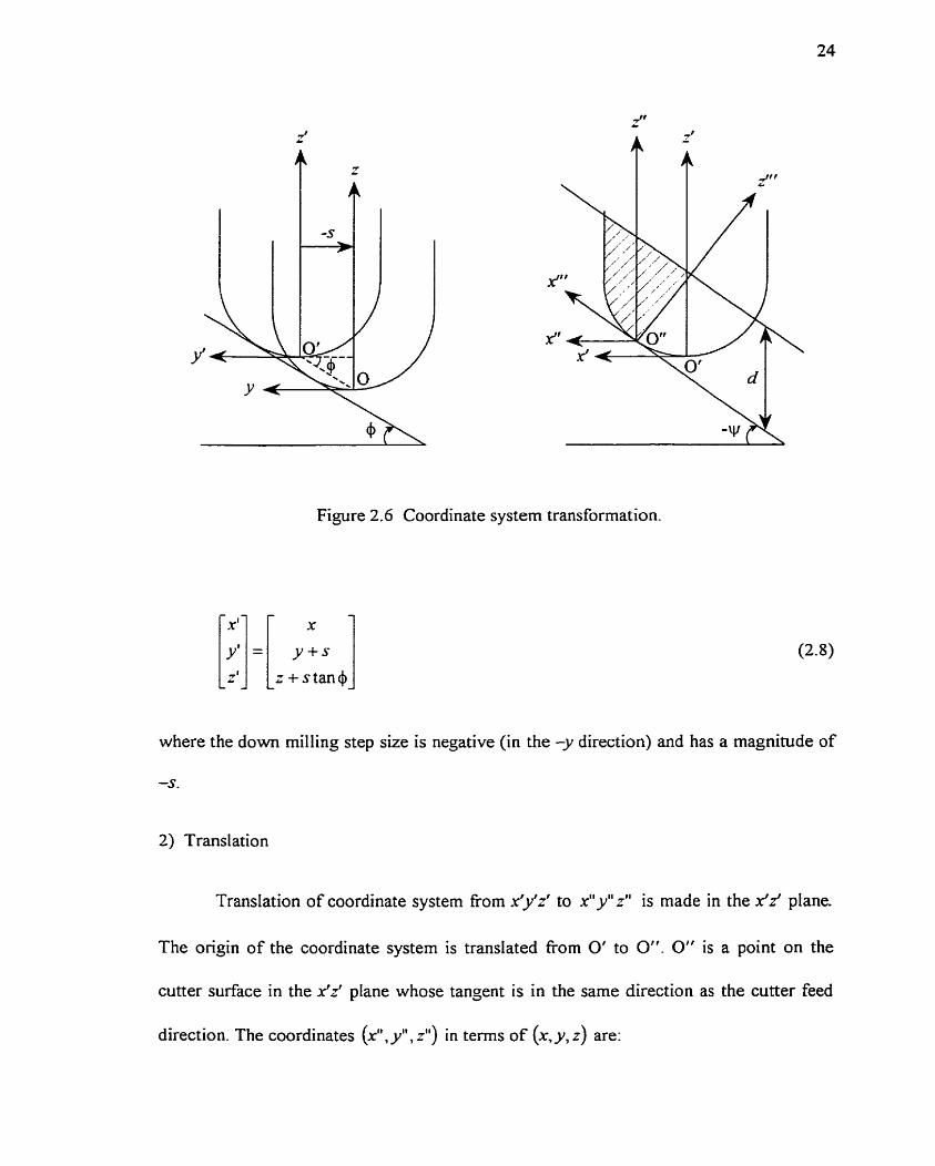
Figure 2.6 Coordinate system transformation.

where the down milling step size is negative (in the -y direction) and has a magnitude of

-S.

2) Translation

Translation of coordinate system from x'y'z' to x" y" z" is made in the x'z' plane.

The origin of the coordinate system is transIated from O' to O". O" is a point on the

cutter surface in the iz' plane whose tangent is in the same direction as the cutter feed

direction. The coordinates (x", y", r") in terms of ( x , ~ , z) are:

xltRsin y

2-(R - R cos y)

x+ Rsin =i Y + S

r+s tan+(R- Rcosiy)

3) Rotation

Rotation of coordinate system x"'y"r" with respect to y" axis by -yr results in

coordinate system x"'y'"z"'.

O 1 O

sin y O cosy

xcosv -=sin y~ - ssin 1~ tan4 t Rsin \y =I Y + S xsin ~ + z c o s y + s t a n ~ c o s ~ y -Rcos \~ /+X

In the yfr'z"' plane, the cross section of the previous dot

surface boundary limit can then be expressed as:

surface is circular. The slot

M?+(~II I -R)? = ~2 if z"'< R (bal1 part of the slot surface) (2.1 la)

y% ,R if z"'> R (cylindrical part of the dot surface) (2.1 Ib)

where y"' and i" cm be obtained from Eq. (2.10). If cutting elements are inside the

boundary limits defined in Eq. (2.1 1) they are not engaged in cutting. For any cutting

element at (Y", y"', Y), the engagement with respect to the adjacent slot surface can be

detemined in the bal1 part and the cylindrical part of the cutter separately:

a) when r' " I R (the bal1 part of the dot surface)

If y""+(z"'-R)' 5 R', the cutting element is inside the previous adjacent slot

surface. It is not engaged in cutting.

If y""+(r"'-R)' > R2, the cutting element is outside the previous adjacent slot

surface. It can be participating in cutting.

b) when z"5 R (the cylindrical part cf the dot surface)

lt' k''i c K , the cutting eiemenr is inside tne prcvious aajacenr dot sudidce. ii is nui

engaged in cutting.

If b"'l> R , the cutting element is outside the previous adjacent slot surface. It can be

participating in cutting.

The non-horizontal feed direction of the cutter results in the third boundary limit:

x=(z-R)tany if z I R (bal part of the cutter) (2.12a)

x=O if z > R (cylindrical part of cutter) (2.12b)

In the cylindrical part of the cutter, this boundary lirnit is the yz plane. The cross-section

of the ball part of the ball-end mil1 in the yz plane is a half circle. The boundary limit set

by the non-horizontal feed direction in the ball part of the cutter is obtained by sweeping

this half circle to an angle w until it reaches the surface generation point Pa about an axis

that passes through (O,O,R) and is parallel to the y axis. T h e half circle plane at this

position is the boundary limit for the ball part of the cutter set by the non-horizontal

cutter feed direction. For both. the bal1 part and cylindricat part of the bail-end miIl,

cutting elements in front o f these two planes (in the x direction) can be engaged in

cutting, while the rest of the cutter is not engaged in cutting. In Figure 2.6, cutting

elements within the shaded area can be participating in cutting. The mathematical

expression for this boundary limit c m be expressed as:

a) when z 5 R (the ball part of the cutter)

If x > ( z - R)tan\y , the cutting element is in front of the non-horizontal feed

direction boundary limit. It can be participating in cutting.

If x < (i - R) tan y , the cutting element is not engaged in cutting.

b) when z > R (the cylindrical part of the cutter)

If x r 0, the cutting element is in front of the yz plane (in the x direction). It can be

participating in cutting.

If x < 0 , the cutting element is not engaged in cutting.

Each of these three boundary limits slices off the unengaged cutting elements

from the cutter. These boundary limits then enclose an area on the cutter surface that

represents the cut geometry. This area includes cutting elements that satisQ al1 the

engagement requirements sirnultaneously. Typical cut geometry in 3D ball-end rnilling is

depicted in Figure 2.7. In this figure, the darker area is the cut geometry. It is very

complicated and used to identie the engaged cutting elements on the ball-end mill.

Undeforrned chip thickness is the radial distance between the path the current

cutting edge element is generating and the machined surface lefi in the immediate

previous cutter revolution at the same angular position. A generalized algorithm is

employed in the present work to determine the undeformed chip thickness for each

engaged cutting element in 3D baI1-end rnilling. It is evident that the path of a milling

tooth is trochoidal. Due to the fact that the cutting speed is much larger than the table

feed rate, the tooth path can be approximated by a circular cunre. Al1 the calculations

related to undeformed chip thickness are based on this assumption. Factors considered in

establishing the cutting element trajectory include cutter runout, cutting system

deflection, and non-horizontal cutter feed motion.

Cutter runout in machining refers to the state of tool cutting points rotating about

an axis different fiom geometrical axis of the cutter. It is an inevitable condition in the

milling processes resulting fiom errors in holding the cutter in the spindle and has been

examined in the form of an offset, a tilt or a combination of both of the cutter axis fiom

the spindle a i s . Figure 2.8 depicts a possible configuration of a ball-end mill and a

spindle. In the lower half of the figure, a cross-section of the ball-end mil1 at z is shown.

p(z) is the cutter axis offset fiom the spindle axis and h(z) is the locating angle that

indicates the direction of the offset at z. If the machining system is completely rigid, the

presence of cutter runout tends to make cutting forces quite asymrnetric in cornparison to

Cut Geometry v

Figure 2.7 Typical cut geometry in 3D ball-end milling.

Section AA

Axis

Figure 2.8 Cutter ninout configuration (Feng and Menq, 1994a).

those without runout. Cutter runout causes the chip load to Vary between cutting teeth

over the rotation of a multi-tooth cutter. It is obvious that with cutter runout, the chip

loads of sorne cutting teeth become larger while the chip loads of some other cutting teeth

become smaller or even zero. This varying chip load will alter cutting forces and result in

asymmetric cutting forces. Cutting system deflection is typical for slender ball-end mills.

Cutting system deflections temper the effecc of runout and reduce peak cutting forces.

The combined effect of cutter mnout and cutting system deflection is to redistribute the

ideal syrnmetnc undeformed chip thickness distribution for the multipie cutting edges. It

often results in a machined surface that is not necessarily generated by the immediate

previous cutting edge in the last cutter revolution. Non-horizontal feed motion of the

cutter further cornplkates the analysis with feed components in the axial as well as the

horizontal directions-

The present undeformed chip thickness determination algorithm is based on the

analysis of trajectones of an engaged cutting element and the corresponding cutting

element on each cutting edge in the immediate previous cutter revolution at the same

angular position. Because of the existence of cutter mnout and cutting system deflection

caused by cutting forces, the surface lefl in the previous revolution may or may not be

generated by the immediate previous tooth. It rnay be generated by any tooth of the cutter

in the immediate previous cutter revolution. The generalized chip t hickness determination

algorithm is to first determine the possible chip thickness candidates and then identify the

correct undeformed chip thickness. The detailed procedure is depicted in Figure 2.9. In

this figure, the cutting element under consideration is on the ith cutting edge, at a distance

r fiom the cutter fiee end, and at an angular position €4 (0, z ) with respect to the y axis,

Figure 2.9 Undeformed chip thickness calcuiation geometry for 3D ball-end milling.

where 8 represents the angular orientation of the cutter. C,, C,.i, C,-2, and Cf-, are the

ideal rotational centers (undeflected spindle centers) of the current cutting element and

the corresponding cutting elernents on the immediate previous, the second previous, and

the mth previous cuding edges. Cutting system deflections caused by the cutting forces

shift the ideal rotational centers to the deflected centers, C',, C', -1, C', -2, and C', -,. 5x3

and Sy's indicate cutting system deflections in the x and the y directions. R,(z) represents

the cutting radius of the cutting element, which is often different from the ideal cutter

radius due to cutter runout, The non-horizontal cutter feed motion results in feed

components in both the x and the z directions, The x component advances the ideal

spindle center t y fcosv in one tooth penod. The z component causes cutting radius

changes for the correspondin: cuttin- el ements on the multiple cutting edges.

Based on the above descriptions, trajectories of the cutting elements shown in

Figure 2.9 can be formulated as

Trajectory = Spindle center position + Cutter deflection + Cutting radius

If the ideat spindle center C, is specified as the reference zero, the radial position of the

current cutting element, 7; (0, z) , at the angular position 8, ( O , z ) can be expressed as

ï; (0, z ) = [6x, sin Oz (8, z ) + 6y, cos€( (8, z ) ]+ R, ( z ) (2.13)

where

In Eq. (2.14), R(z) is the ideal cutter radius at z. R(r) changes with r in the bal1 part of the

cutter and remains uniform in the cylindrical part of the cutter:

R(z) = JZRZ - r' O r z I R (bali part of the cutter)

R(z) = R t > R (cylindricat part of the cuiter)

N is number of cutting edges of the cutter, p(r) and A(=) are parameters characterizing the

cutter runout (Feng and Menq, 1994a), j3 is the helix angle of the cutter, and 9 is the

angular position of tooth number 1 (arbitrarily selected) at the cuaer free end (z = 0) .

The radial position of the corresponding cutting element on the mth previous

cutting edge in the last cutter revolution at the same angular position is given by

1;-,(O,=)=-mf cos~sin9,(0,~)+[âr,~,sin9,(~,r)+6y~~mc~~Bi(8,z)]+

R,-, ( z - mf sin y) (2.16)

The radial position difference between the current cutting element and the

corresponding cutting element on the mth previous cutting edge at the same angular

position forms an undeformed chip thickness candidate. This candidate, t,, is obtained

by subtracting Eq. (2.16) from Eq. (2.13):

For a ball-end mill of N cutting edges, N undeformed chip thickness candidates can be

obtained using Eq. (2.17). The correct undeformed chip thickness is the smallest positive

one of the N candidates (t2 in Figure 2.9). If a11 of the N candidates are negative, the

undeformed chip thickness is zero. This indicates that the current cutting element is not

cutting any material at this particular angular position due to the combined effect of cutter

runout and cutting system deflections.

It should be noted that, for cutting elements close to the cutter fiee end, the

corresponding cutting element on the previous mth cutting edge does not always exist.

This occurs when the ba11-end mill is feeding with a negative z component and

Ri_, (z - mf sin W) = O (or z - mf sin y r O )* In this situation, the undeformed chip

tiïickness canciiciate is given 'oy

Having established the undeformed chip geometry for a given cutter orientation

fio m the cut geometry and the undeformed chip thickness detemination procedure, the

instantaneous cutting force is readily obtained using the empincal chip-force

relationships. Empirical chip-force relationships in metal cutting are established based on

extensive experimental studies. They relate the cutting forces to the undeformed chip

geometry. Researchers have used different but similar empirical relationships to mode1

cutting mechanics in the multi-toothed milling processes. The empirical chip-force

relationships employed in the previous work by Feng and Menq (1 994a) were

where dF, and are the diffierential tangential and radial cutting force components,

dz the axial depth of cut, and ri ( 0 , ~ ) the undeformed chip thickness of the cutting

element at 8, ( 0 , ~ ) . K,(r) and KR(;) charactenze the cutting mechanics of the

differential cutting eiements at z. In Eqs. (2.19) and (2.20), size effect in metal cutting

Wakayama and Tamura, 1968) is explicitly considered. The size effect is the effect of

undeformed chip thickness on the unit horsepower and specific energy values needed for

the machining processes. As undeformed chip thickness t , (0, r) is reduced, power and

energy requirements to machine the same undeformed chip area increase. This

relationship is referred to as the size effect (Groover, 1996). In Eqs. (2.19) and (2.20), the

mode1 parameters rn, and m, , which basically charactenze the size effect of machining

the workpiece material, are assumed to be constant for a particular material. For most

metallic materials, m, and m, are both greater than O and Iess than I (Le., O < mT < 1

and O < rn, c 1). The importance of including size effect in modelling slot milling

operations has recently been demonstrated (Melkote and Endres, 1998).

The empirical parameters KT ( z ) , KR ( z ) , m, , and m, were obtained fiom a set

of horizontal slot cuts. Venfication experiments have shown that Eqs. (2.19) and (2.20)

provide reliable cutting force predictions for horizontal cuts (Feng and Menq, 1996).

Nonetheless, for non-horizontal cuts typical in 3D bail-end milling, the empirical chip-

force relationships are likely to be insuffkient. To achieve accurate cutting force

prediction in non-horizontal ball-end milling, non-horizontal cutting mechanics should be

considered. Ideal chip-force relationships considering the cutter feed angle w would be:

The cutting mechanics parameters KT and KR are expressed as functions of v as well as

r in order to deal with the chip flow direction changes in non-horizontal cuts. The exact

hnctional forms of KT (v,r) and KR(y,z) cm b e quite cornplex and it will require

extensive experimental tests to deterrnine the empirical coefficients. The amount of the

experimental test cuts can be dramatically reduced if the effects of the variables y and z

on the cutting mechanics are independent with each other such that K,(v,z) and

K R (11, r} can be expressed as

Equations (2.23) and (2.24) are in fact reasonable approximations to K,(y,z) and

KR(v, z ) . The correlation between the effects of y and r on the cutting rnechanics is

minor in that the former is process-based (characterized by the cutter feed direction of the

ball-end milling process) while the latter is cutter-based (characterized by the cutting

edge design of the ball-end milling cutter). Introducing Eqs. (2.23) and (2.24) to Eqs.

(2.2 1) and (2.22) results in

The main advantage of Eqs. (2.25) and (2.26) can be observed from a comparison

with Eqs. (2.19) and (2.20), the empirical chip-force relationships used previously.

KT., (w) and KR, (w) are the newly introduced terms to characterize non-horizontal

cutting mechanics in 3D ball-end milling. The rest of the formulation is the same. As a

result, the experimental procedure to determine the empirical model parameters is greatly

simplified as will be described in the following section.

2.2.4 Crrtting Force Caladatior,

In the mathematical procedure to calculate the cutting forces, an iterative

procedure is employed to obtain equilibrium chip geometry and cutting forces. Since the

deflection-dependent chip geometry can only be established if the cuaing forces are

known at any 0 over the last full cutter revolution, for any 8, initial values are first

assumed for the cutting forces the model is intended to predict. Once the cutting forces

are assumed, the resulting chip geometry can be obtained. With this obtained chip

geometry, the new cutting forces are calculated. The cutting force information is updated

by companng the calculated cutting forces with the initially guessed cutting forces, and

this iterative procedure continues until the difference between the guessed cutting forces

and the calculated cutting forces is within specified convergence criteria.

2.3 Determination of Empirical Mode1 Parameters

Empirical model parameters in Eqs. (2.25) and (2.26) need to be determined in

order to use the present model to calculate cutting forces in 3D bail-end milling. The

empirical parameters KT .- . ( z ) , KR, (r), m, , and rn, cm be obtained from horizontal siot

cuts with KT.,(0) = 1 and KR-,(O) = 1 using the same model building procedure

described before (Feng and Menq, 1994a). The values of K,,(y) and K,,(y) for

w r O are determined From measured average cutting forces of non-horizontal slot cuts

based on the mathematical procedure shown below.

To obtain the cutting forces acting on the ball-end mil1 at any instant, the

riemeniai iangenciai anci radiai curring forces are resoived inro the x, y ciireciions and

summed over al1 the engaged differential cutting edges. The summation (integration) is

done numerically along the z-axis to yield the instantaneous forces in the x, y directions:

From Eqs. (2.27) and (2.28) the averqe cutting forces in the x and y directions of a ball-

end mil1 cutting with a feed angle can be expressed as

where

(2.3 la)

(2.3 1 b)

(2.3 Ic)

When cutting system deflection is not considered, for the particular case of dot cut

machining, the variation of the undeformed chip thickness over a full cutter revolution is

symmetric to the x axis for each differential cutting edge element. Because of the anti-

symmetry of the cosine fùnction to the same axis, the tangential and radial mode1

parameters are decoupled and can be determined independently (as shown by Feng and

Menq, 1994a). Under this situation a0 and cl are equal to zero. Due to the consideration

of cutting system deflection in the determination of undeformed chip thickness, the

variation of the undeformed chip thickness over a full cutter revolution is no longer

symmetric to the x axis. The tangential and radial parameters in Eqs. (2.29) and (2.30) are

not decoupled any more. So, to obtain K,, and KR-,, numerical integration bas to be

cam-ed out for each item formulated in Eq. (2.3 1). The coefficients a,, a, , c, , and c, are

calculated using the empirical parameters KT .- . ( z ) , KR.= ( z ) , mT , and m, determined

previously. These coefficients are then used in Eqs. (2.29) and (2.30) with the measured

- F, and to solve for the values o f KT-, and KR, for the particular y.

Two non-horizontal slot cuts were carried out using the same bail-end mil1 and

workpiece matenal a s in the previous work (Feng and Menq, 1994a). The detailed

cutting conditions were = +jOO, 4 = O", d = 6.3 5 mm, and v = 45.72 m d m i n (f =

0.038 1 mdtooth) . Slot cuts were used since they resulted in symmetric undeformed chip

genmetry wirh respect ?Q fk x zxis In ne c-t?er re~o!-tI~n for the rigirl hl!!-end mi!!ing

system and nearly symmetric undeformed chip geometry for the flexible system. The

resulting values of the coefficients formulated in Eq. (2.3 1 ) are shown in Table 2.1. As

expected, the values o f a, and c, are negligibly small compared with those o f a, and c, .

This indicates that KT.,(\v) and KR-,(iv) are in effect decoupled in Eqs. (2.29) and

(2.30) and can be determined independently.

This procedure has generated two sets o f values for KT.,(v) and &,(w):

KT.v = 0.97, KR-, = 1.16, for = 30"; and K ,-,,, = 1-09, = 1 -06, for w = -30". These

values represent the effect o f the chip tlow direction changes in non-horizontal cuts on

the cutting mechanics. They are used to calculate cutting forces in 3D ball-end milling

with y = k30°. Values of KT., and KR., for different u, can be obtained using this

procedure. Empirical functional expressions will be developed when suficient data

become available.

Table 2.1 Values of the coefficients formulated in Eq. (2.3 1) for the two non-horizontal

slot cuts,

2.4 Mode1 Validation and Discussions

The present mode1 has been validated by comparing the predicted and the

measured cutting forces in 3D ball-end milling. The measured cutting forces were

obtained fiom a set of steady stat- non-horizontal and cross-feed cuts of a ball-end mill.

The workpiece material used was S M 10 18 cold-rolled steel. Union ButterfieId M42

Cobalt HSS ball-end mills with 12.7 mm diameter, 2 Butes and 35" helix angle were used

as the cutting tools in the experiments. The detailed experimental setup has been

illustrated in the previous work (Feng and Menq, 1994a). Predicted cutting forces were

calculated using the current mode1 and the previously developed flexible system mode1

(Feng and Menq, 1996). The test conditions of the experiments comprised of down

milling cross-feed cuts and horizontal and non-horizontal cuts. Cross-feed cuts and non-

horizontal cuts were tested because they illustrated more closely the actual action of a

bal 1-end mi 11 used in 3 -axis milling. Cross-feed cuts are required to generate satisfactory

surface finish on the machined surface. Non-horizontal cuts are indispensable if a 3-axis

NC machine is used to generate a 3D scuiptured surface. The detailed cutting conditions

of the tests are iisted in Table 2-2.

Table 2.2 Detailed cutting conditions for rnodel verification test cuts.

Test Milling Feed per tooth Depth of Cut Step Size W 4) No. Type (mmltoot h) (mm) (mm) (deg-) (deg-)

1 down 0.038 1 6.3 50 -3.175 O -15

2 down 0.038 1 6.286 -3.175 +3 O O

3 down 0.03 8 Z 6.286 -3.175 -3 O +15

4 d o m 0.03 8 1 6.286 -3.175 +3 O -15

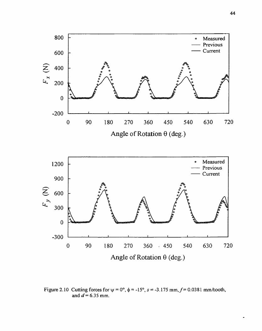
First, a horizontal cut is carried out to show the ability of the present model in

predicting cutting forces for horizontal cuts. Figure 2.10 (test No. 1) shows cutting force

predictions of a horizontal down milling cut with a downward 15" cross-feed. As pointed

out before, the previous model (Feng and Menq, 1996) gives excellent predictions of

cutting forces in horizontal cuts. Modifications are made in the current mode1 to deal with

non-horizontal cuts. The applicability of both the previous and the current models in

horizontal cuts can be seen in the figure. In the current model, horizontal cuts can be

treated as special cases in which y = O". Therefore, cutting force predictions for

horizontal cuts in the current model should be as good as those in the previous model. In

Figure 2.10, the heavier lines represent the current predicted cutting forces, while the

thinner lines represent the previous predicted cutting forces. It can be seen that these two

lines overlap each other. As expected the predicted cutting forces in the current model are

O Measured Previous

- Current

90 180 270 360 450 540 630 720

Angle of Rotation 8 (deg.)

O Measured Previous Current

O 90 180 270 360 - 450 540 630 720

Angle of Rotation 8 (deg.)

Figure 2.10 Cutting forces for w = O", $ = -lSO, s = -3.175 mm, f = 0.038 1 mdtooth, and d = 6.3 5 mm.

exactly the same as those in the previous mode1 and in good agreement with the

measured cutting forces.

Test No. 1 is also used to show the effect of cutter runout on cutting forces. Figure

2. L 1 is the cornparison of predicted cutting forces with cutter runout and without runout

using the current model. The thicker lines represent the predicted cutting forces with

cutter runout while the t h i ~ e r lines represent the predicted cutting forces without cutter

ninout. When cutter runout is not taken into account, the predicted cutting forces are

symmetric. The peak force in the x direction at 8 = 170" is equal to that at 8 = 3 50° . Due

to the presence of cutter runout, chip load on one tooth is larger than that on the other

such that the cutting forces become asymmetric. In one cutter revolution (0=0°-360°),

the peak force at 8 = i7ù2 becomes iiigiier tiian that witiiout cutter runour. On the otner

hand, the other peak force at 8 = 3 50" is lower than the corresponding one without cutter

runout. The same observation is also made for cutting forces in the y direction. In

practice, cutter runout is inevitable. To refiect the real characteristic of the rnilling

processes, it is important to include cutter runout when modeling cutting forces. It has

been shown in Figure 2.1 1 that the inclusion of cutter runout in the cutting force model

gives better cutting force predictions.

Figure 2.12 (test No. 2) shows the predicted results of a non-horizontal cross feed

cut camed out to show the suitability of predicting instantaneous cutting forces using

coefficients obtained from measured average cutting forces of dot cuts. In the current

model the newly introduced model pararneters K,.,(w) and K,.,(w) are established

from measured average cutting forces of non-horizontal slot cuts. The step size in test No.

0 Measured Without runout With ninout

Angle of Rotation 8 (deg.)

O Measured Without runout With runout

O 90 180 370 360 450 540 630 720

Angle of Rotation 9 (deg.)

Figure 2.11 The effect of cutter mnout for \y = O", 4 = -1S0, s = -3.175 mm, f = 0.038 1 mmkooth, and d = 6.35 mm.

Measured Previous

- Current

O 90 180 270 360 450 540 030 720

Angle of Rotation 0 (deg.)

O Measured Previous Current

O 90 180 270 360 450 540 630 720

Angle of Rotation 0 (deg.)

Figure 2.12 Cuttingforces for = 30". 4 = 0°, s = -3.175 mm, f = 0.0381 mmftooth, and d = 6-286 mm.

2 is K of the cutter diameter. It is shown that the predicted results in the previous model

are not even close to the measured one, especially for the y cutting forces. Remarkable

improvements can be found in instantaneous cutting force predictions in the current

model. These results have shown that coefficients obtained fiom average cutting forces of

sIot cuts are suitable in predicting instantaneous cutting forces.

Figures 2.13 (test No. 3) and 2.14 (test No. 4) show two other cutting force

compansons. Figure 2.13 represents a 3D ball-end milling cut where the cutter feeds

upward at an angle of 30" and cross-feeds in the -y direction (down rnilling) at an upward

angle of 15" and with a step size equal to !A of the cutter diarneter. Figure 2.14 is for a

cut with a downward 30" feed and a downward 15" cross-feed.

It can been seen nom Figure 2.13 that the current predicted results are similar to

the previous ones. Both predictions are in gmd agreement with the measured results.

Some irnprovements of the present model are observed for the relatively small x forces.

The asymrnetric cutting force waveforms of the two cutting edges are evident and this

results fiom the combined effect of cutter runout and cutting systern deflections. Figure

2.14 shows the significant improvernent of the present model cornpared with the previous

one. The previous predicted cutting forces only follow the general trend of the measured

forces. Prediction inconsistency is seen to exceed 700 N in some areas. The present

model provides excellent cutting force predictions. It accurately predicts fine details of

the measured force signals. The onset of cutter engagement is shown as tuming points in

the cutting force waveforms in Figure 2.14. The measured x force signal shows a turning

point around 0 = 150". The present predicted value is almost identical to the rneasured

O Measured Previous

- C urrent

O 90 180 270 360 450 540 630 720

Angle of Rotation 9 (deg.)

a Measured Previous

- Current

O 90 180 270 360 450 540 630 720

Angle of Rotation 8 (deg.)

Figure 2.13 Cutting forces for w = -30°, 4 = 1 SO, s = -3.175 mm, f = 0.03 8 1 mmhooth, and d = 6.286 mm-

Measured Previous

- C urrent

O 90 180 270 360 450 540 630 720

Angle o f Rotation 8 (deg.)

1200 O Measured

- 900 Current

600

Lr? 300

O

-300

O 90 180 270 360 450 540 630 720

Angle of Rotation 8 (deg.)

Figure 2.14 Cutîing forces for w = 30°, 4 = -lSO, s = -3.175 mm, f = 0.038 1 mrn/tooth, and d = 6.286 mm.

one while the previous modet predicts a turning point around 8 = 90". Similar

observations can be made for the y cutting forces.

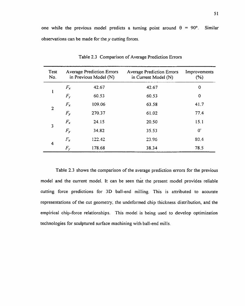
Table 2.3 Cornparison of Average Prediction Errors

Test Average Prediction Errors Average Prediction Errors Improvements No. in Previous Mode1 (N) in Current Mode1 (N) (%)

Table 2.3 shows the cornparison of the average prediction errors for the previous

mode1 and the curent model. It can be seen that the present model provides reliable

cutting force predictions for 3D ball-end milling. This is attributed to accurate

representations of the cut geornetry. the undeformed chip thickness distribution, and the

empirical chip-force relationships. This model is being used to develop optimization

technologies for sculptured surface machining with ball-end rnills.

CHAPTER 3

INTEGRATED PROCESS PLANKING BASED ON CUTTING

FORCE OPTIMIZATION

3.1 Introduction

Process planning is a manufacturing activity generating production information

£tom design information. It is aimed at determining the most economical rnanufacturing

process for producing a part with high quality. As cutting forces are directly related to the

process efficiency and product quality, optimization of cutting forces in machining

prùctraes piàys ari iiripor~arii d e in process pianning. The optimum curting forces shouid

be maintained in the machining process so as to achieve the highest efficiency. Optimum

process parameters such as maximum feedrate are selected based on the machining errors

caused by cutting forces. Process planning in 3D surface machining using ball-end

rnilling primarily involves two procedures: tool path determination and maximum

feedrate selection. Tool path is directly related to the surface geometry and feedrate

specifies the speed of the tool moving along the tool path. Tool path planning requires

speciQing cutter feed directions and step sizes between adjacent tool paths for the cutter

to generate the product geometry. The aliowable scallop height on the machined surface

determines the maximum step size for each cutter feed direction. Feedrate selection

directly affects machining errors caused by cutting forces and cutting system deflections

in end milling. As cutter feed direction and step size change, cut geometry and the

resulting cutting forces change. This leads to changes in maximum feedrate so that the

resulting machining errors can be maintained within the specified tolerance lirnits.

Optimization of the machining process is achieved when the rnachining time required to

manufacture the product is minimum. The machining process planning procedure c m

thus be interpreted as a machining time minimization procedure subjected to the

constraint of the product quality requirements.

Much work has been done in the past in the area of adaptive control of the milling

processes. However, implementation of such on-line adaptive control systems in

industrial settings is often very dificult. The process planning approach presented herein

is an off-line optimization procedure. It is clear that in this ofNine optirnization

procedure if the machined product quality can be predicted prior to actually cutting the

~ Ü ~ C Z , ï~âdïiiiiiig p:onîGiig câii bs iiitd:ig~iiiIj: c û i i d ü ~ ~ d tû zchiere hiohci p iûûù~i i i ty

and better product quality simultaneously. To achieve this, models to predict the cutting

forces, tool deflections, and machining errors of the machining process are required. The

cutting force mode1 developed in Chapter 2 provides a valuable tool for this purpose. In

the finishing machining of 3D plane surfaces, tool path determination and maximum

feedrate selection are interrelated and interact with each other. Determination of one

should not be independent of the other.

For a given 3D plane surface, there exist many machining process plans with

which the part can be machined within tolerance requirements. Of al1 the possible

machining process plans, only the one with the minimum time and relatively small

machining errors is chosen as the optimai machining process plan in this new process

planning approach. In search for such an optimal machining process, the maximum step

size, the maximum feedrate, the total tooI path length, the machining errors, and the

resulting machining time need to be analyzed and compared.

3.2 Mathematical Formulation

Numerous process pIans exist to machine a 3D plane surface using ball-end

milling that are able to meet the scallop height and tolerance requirements. The.optirnum

machining plan requires the least machining time. Figure 3.1 illustrates the components

essential to the determination of machining time for the finishing machining of a 3D

plane surface. It is evident that parallel tool paths will be used to generate the plane

surface geornetry. For a particular cutter feed direction, maximum step size between the

parallel tool paths is determined from the scallop height requirement based on the cutter

geometry and the plane surface orientation. Total tool path Iength can then be calculated

fiom the given plane surface geometry and the established maximum step size. Maximum

feedrate is determined f?om the tolerance requirement using the cutting force mode1

described in Chapter 2. Machining time for the particular feed direction is readily

available from the total tool path length and the maximum feedrate. The minimum

machining time corresponds to the optimum feed direction. The corresponding tool path

and feedrate then constitute the optimum process plan. The components invoived in

Figure 3.1 are descnbed in more detail in the following sections.

3.2.1 Feed Directzor?

Feed direction represents the moving direction of the cutter dong the tool path. It

is a constant in the finishing machining of 3D plane surfaces due to parallel tool paths.

Two Cartesian coordinate systems are used to specie the cutter feed direction: the part

Feed Direction

a

Cutter Information

3D Plane Surface

I I

Machined Surface Requirements 1 I I I I

ScaIlop Height

1 I

Tolerance u I I I I 1

Cutting Force Mode1

Figure 3.1 Machining time calculation procedure.

coordinate system and the cutter coordinate system. The part coordinate system is used to

define the geometry of the 3D plane surface. There is no restriction on the selection of the

ongin of the part coordinate system. It should be selected for the purpose of convenience.

The cutter coordinate system is defined according to the cutter position and the feed

direction. The detailed definition of the cutter coodinate system can be found in Section

Figure 3 -2 depicts these two coordinate systems. The coordinate system with the

upper case letters AT is the part coordinate system. The one with the Iower case letters

xy; is the cutter coordinate system. It is noted that the z directions in both coordinate

systems are the same. From the definition of the cutter coordinate system, it is clear that

a in the XY plane in defining the cutter feed direction is introduced in this work. It

represents the angular displacement between the cutter and the part coordinate systems.

The range of a is 0° to 360". The definition of a is shown in Figure 3.2. In this figure, Po

is the cutter contact point with the surface (surface generation point). As the feed

direction (a) changes, the ball-end mil1 follows different tool path to generate the plane

surface. This results in changes in the cut geometry of the bali-end mil1 and thus changes

in cutting forces, cutting system deflections, and the resulting machining errors. The

coordinates of Po in the cutter coordinate system are required to formulate the cut

geometry. They Vary with the feed direction. Let (Xo, Yo, 20) represent the coordinates of

Po in the cutter coordinate system for a = 0' (the determination of X-J, Yo, and Zo is

described in detail in Appendix A). The coordinates of the cutter contact point Po(x0, yo,

ZO) in the cutter coordinate system at any feed direction a can be expressed by

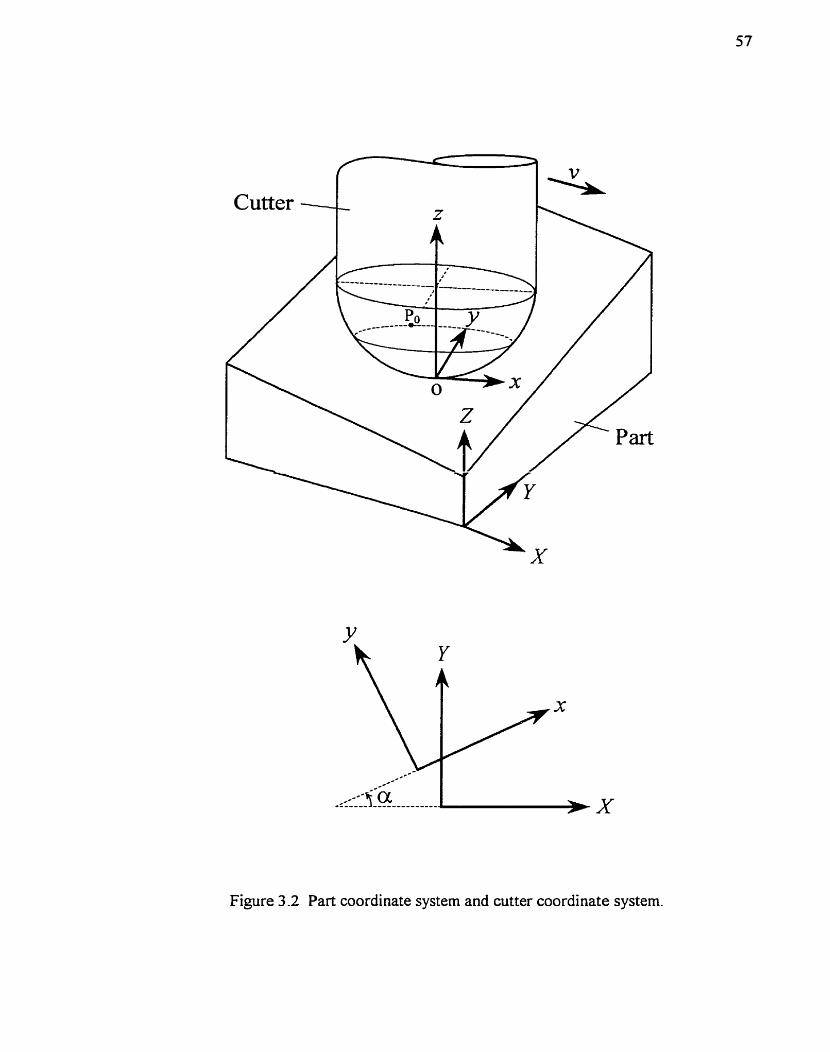
Figure 3.2 Part coordinate system and cutter coordinate system.

As discussed in Section 2.2.1, the cut geometry is characterized by angles yl and

9. It is evident that w and 4 change with respect to the cutter feed direction (cc) as xo and

y0 change with a. For one particular Pa, the corresponding feed angle and cross feed

angle 4 at a are given by Eqs. (2.2) and (2.3) and re-written as

Changes in y and 4 result in changes in cut geometry, and therefore lead to changes in

cutting forces.

Step size represents the distance between two adjacent tool paths in the y direction

of the cutter coordinate system. It determines how far in the cross feed direction the cutter

moves to machine the next tool path so that the machined scallop is smaller than the

requirements. Changes in step size affect the cut geometry of the ball-end mil1 and the

size of the scallop lefi on the machined surface. Step size is kept constant between the

parallel tool paths in 3D plane surface machining to produce constant scallop height and

to maximize eficiency. It is evident that maximum step size reduces the total tool path

length for a specific cutter feed direction. Step size plays an important role in machining

time calculation because it is not only related to the total tool path length but also related

to the maximum feedrate. Changes of step size resuIts in variations in the total tool path

length and the maximum feedrate.

Given the scallop height requirement of a 3D plane surface, the maximum step

size varies according to changes of and 4. Step size for a given scallop height is readiIy

detemined in the normal direction of the 3D plane surface. Figure 3.3 shows the step size

caIculation procedure. The xy,- coordinate system is the original cutter coordinate system.

As the scallop height is rneasured in the surface normal direction, if the original cutter

coordinate system is used, the step size calculation procedure will become very

complicated. To reduce the diffrculties in calculating step size, coordinate systern

L--ir--.-i -.. -- (.....;- P: -..-- 9 - \ - 1 . . . .I. J . - ,,-, . ,, LI a~isiui iiiaiiuii~ &le ~ à i ï i i d r i ~ u i ti 3 .>ta) iiiusii aics L L I ~ GUUL U I ~ I L C : S Y S L C I ~

transformation procedures needed to calculate the step size:

First, the .yz coordinate system is translated in the xi plane to the point on the

cutter whose tangent is at an angle of i y with the x axis. The coordinate system is now

x'y'r'. The coordinates (xo, yo, zo) of Po in the original cutter coordinate system now

become (xor7 yor, a') in the translated coordinate system x'y'z' :

x, + Rsin w

-0 z, -(R-RCOSV)

Second, rotation of an angle of iy is made about the y' axis and the coordinate

system rotates from x'y'z' to x"Yir. After the rotation the cross-section of the bal[ part of

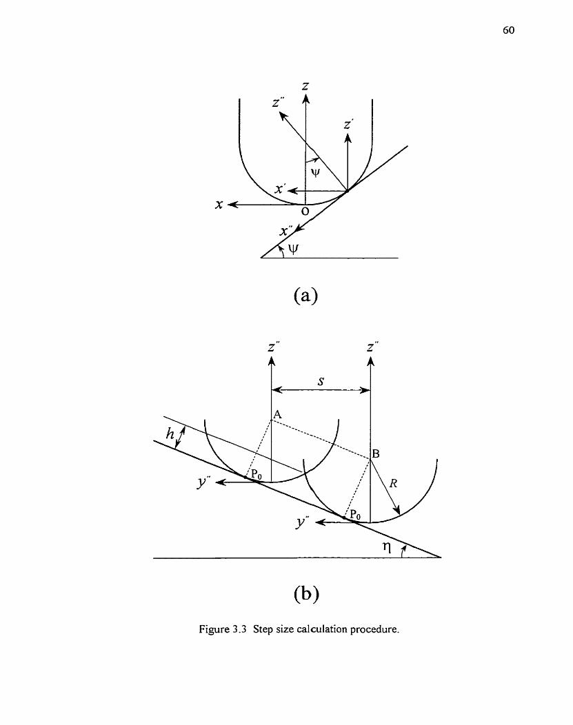
Figure 3.3 Step size calculation procedure.

the cutter on y".$' plane is a half circle. The coordinates of the cutter contact point PO

become (xo", y& =O"):

It can been seen that after the coordinate transformations the y coordinate value does not

change, while x and r coordinates change. As s h o w in Figure 2.3, before the coordinate

system transformations, on the plane parallel to the yz plane and containing Po, the

tangent to Po is at an angle 4 with the y axis. The corresponding angle in the transformed

coordinate system x''y"i' is no longer equal to 4 and denoted as q. q can be forrnuiated as

,IR' -Y, 2

q = cos-' R

Figure 3.3(b) depicts the determination of the step size. In the transformed

coordinate system Y r ~ i ' , when the bal1 part center of the cutter moves h m B to 4 the

distance between these two centers in they" direction is the step size S. h represents the

scallop height in the plane normal direction, while Po is the cutter contact point with the

surface. The step size can be expressed as

s = 2cosq J z R ~ - h 2

The detailed derivation of step size s is descnbed in Appendix B.

3.2.3 Feedrate

In machining operations, feedrate represents the speed of the cutter moving in the

feed direction relative to the workpiece. Feedrate selection directly affects the eficiency

of the machining process and the part quality. It is obvious that faster feedrate results in

higher eficiency. On the other hand, faster feedrate leads to poorer part quality due to the

large cutting system deflections caused by excessive cutting forces. Constrained by the

surface tolerance requirements, cutting forces can not exceed the Iimiting values. Since e

feedrate is directly related to cutting forces, there are upper limitations for the allowable

feedrate during the machining process. For an end mil1 with N cutting edges. the feedrate,

v, can be calcutated by:

where f is the chip load (feed per tooth) and S is the spindle speed. N is fixed for a given

cutter. S is optimized with respect to cutting speed and tool life. As a result, feedrate

optirnization is in fact a procedure of optimizing the chip load. Chip load f is an essential

parameter to cutting forces. Its optimal value is obtained fiom cutting force and

machining error calculations using an iterative procedure. Cutter feed direction and

maximum step size determined previously are required to calculate the cutting forces.

The cutting forces used to determine the resulting machining errors are those when the

cutter is generating Po on the plane surface. As the ith cutting edge is generating Po, the

angular orientatiofi of the ball-end mil1 is denoted as 9,:

3 27T + z t a n B + ( i - 1)- Bi = sin -' d--

xo +Y, R N

Arnong the N cutting edges, only the cutting edge that produces the largest cutter force

when generating Po is considered. Cutting forces of this cutter orientation are calculated

which are used to iteratively determine the maximum feedrate. It is evident from Eq.

(3.9) that Bi is related to the cutter contact point with the 3D plane surface. As has been

shown in Eq. (3.1), when a changes, the values of xo and y0 change. This results in the

change of 0, according to Eq. (3.9). More irnportantly, cutting force components

calculated at Bi change accordingly.

The surface tolerance which is defined in the surface normal direction is an

importafit criterion in the calculation of the maximum feedrate. Machining erron mainly

result from cutting system deflections in ball-end milling and are measured in the surface

normal directions. The machining error is the component of the cutting system deflection

in the surface normal direction. In other words, the machining error is the inner product

of cutting system deflection and the unit vector h of the surface normal. The

resulting machining error e is then given by:

This machining error is to be evaluated against surface tolerance requirements. To assure

product quality, e rnust be less than the surface tolerance.

Iterative procedure is applied to determine the maximum chip load f: First, a

preset initial value off is used. Cutting forces and the resulting deflections in the x and

the y directions are calculated based on this f using the cutting force mode1 described in

the previous chapter. The machining error is calculated fiom the inner product of the

cutting system deflection and the surface normal vector. Whenever the difference

between the surface toIerance and the calculated machining error is iarger than the

specified convergence criterion, f is updated according to this difference. Cutting forces

and cutting system deflections are re-calculated with the updated f. This iterative

procedure continues until the calculated machining error is very close to the specified

surface tolerance requirement. In other words, the converged f is found when the

projection of the cutting system deflection in the surface normal direction of the 3D plane

surface is equal to the specified tolerance.

It should be noted that often the chip load f can reach a relatively large value

without resulting in significant machining errors. This happens when cutting forces are

smd! 2s the -"'ter is gezerzting Pu md'cr the Z G ~ U ! -;cctcr cf the P!JX S Ï ~ ~ Z C Î i~ z!rncs!

perpetidicular to the cutter xy plane. A typical example is that the machining error of a

horizontal plane is practically zero because the projected error of the cutting systern

deflection is zero. Under these situations, the calculated feedrate can be very large or

even infinite. Using these calculated maximum feedrate in practice is not realistic. Even

though the resulting machining errors are small at the cutter contact point, cutting forces

in other cutter orientations may be very large. In these cases, the maximum chip load

value recommended by machining handbooks (e-g., Tool and Manufacturing Engineers

Handbook, 1983), fm,, is used to avoid tool breakage or chatter. In the current work,

whenever the converged f exceeds the maximum value recomrnended by machining

handbooks, f,, is used as the feed per tooth in the calculation of feedrate.

The machining time for one particular feed direction is readily available fiom the

total tool path Iength and feedrate. The approach to calculate the total tool path length is

depicted in Figure 3.4. Cutter feed direction and maximum step size are used to define

the parallel tool paths on the 3D plane surface. The basic idea is to calculate the projected

tool path length on the xy plane first, and then calculate the tool path length on the 3D

plane surface. The tool path determination procedure is as follows. First, a series of lines

parallel to the x axis in the cutter coordinate system are used to intersect the projected

area of the part in the xy plane. The distance between any two adjacent parallel lines is

equal to the maximum step size S. Second, determine the lengths of these intersected lines

-+vithi:: the prcjectîd r x . Triri, detîni.ix the tm! p-th !r@x c:: the 3E p ! r x s=rf.ce.

Several factors need to be considered in the determination of the tool path lengths.

The first one is the machined scallop heights in the beginning and the end of the

machining process. It should be clear from Figure 3.3 that at the beginning or the end of

machining, when the distance between the cutter contact (CC) tool path and the plane

surface edges in they direction is less than s/2, the resulting scallop height is less than the

maximum scallop height. On the other hand, if this distance is Iarger than d2 , the

resulting scallop height is larger than the maximum scallop height. Therefore, to

eliminate unnecessary cutter movernents, the first intersecting line begins at a distance of

5-12 in the y axis direction with respect to the plane surface edge. At the end of machining,

if the distance between the plane surface and the last intersecting line is larger tlian s/2,

an additional tool path is needed to make the scallop height less than the maximum

scallop height. Othenvise no additional path is needed.

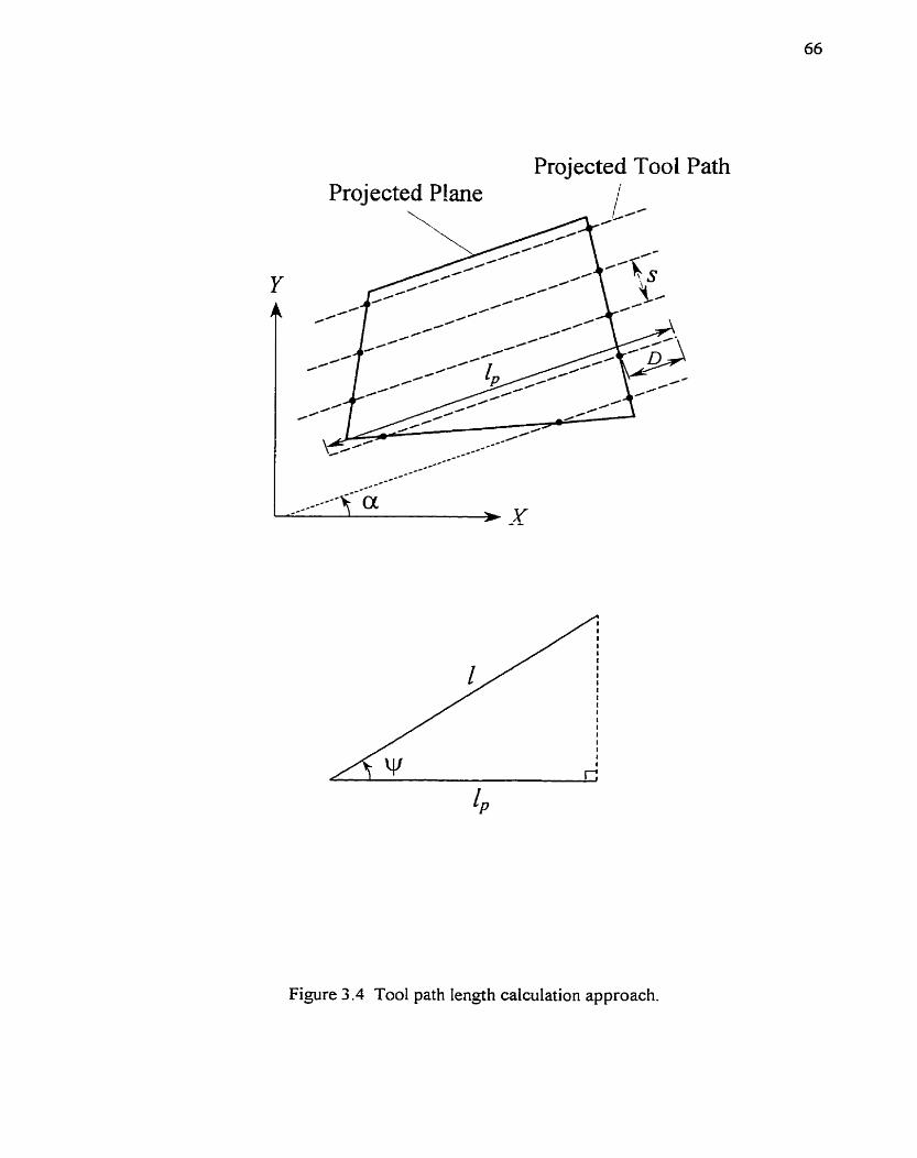
Projected Tool Path Projected P!ane /

Figure 3 -4 Tool path length calculation approach.

Another factor that should be taken into account is the entry and the exit extension

distances from the plane surface. In practice, the cutter starts and ends cutting at

recommended extension distances away frorn the part to provide clearance to the

machined surface. Entry and exit distances are in fact part of each individual tool path.

The entry and the exit extension distance used in the present work is the cutter diameter

D. Therefore, a distance of 2D should be added to each projected tool path length.

In this work, lace (zigzag) or non-lace cut patterns can be used. In non-lace

machining, the cutter rnoves in one direction only. After the cutter finishes machining

one path, it moves rapidly to the start position of the next path. This rapid tool movement

is ignored in the caIculation of machining time because of the rapid feedrate. In other

path is not considered in the calculation of the machining time.

So far, by considering al1 the factors discussed above, the projected tool path

length IF in the xy plane can be calculated. By projecting 1, onto the 3D plane surface by

the feed angle y, the individual tool path length, 2, can be detemined:

[P [=- cos \y

Summing up al1 the individual tooi path lengths yields the total tool path length L.

Once the total tool path length L and the maximum feedrate v for one particular

cutter feed direction are available, the machining time, t, for this feed direction can easily

be deterrnined:

3.3 Simulation Results and Discussions

A simulated machining operation is used to demonstrate the feasibility of the

current process planning method. The geometry of the 3D plane surface is described by a

general plane expression: Ax + By + C: + D = O . (A, B, C) is the plane normal vector.

The 3D plane normal vector used in the sirnulated study is (0.5,0.5,1 .O). The projected

area of the plane surface on the XY plane is a 100 mm x 100 mm square. A ball-end mil1

with 12.7 mm diarneter, 35" helix angle, and two cutting edges is used. Cutting

conditions for the simulated down milling cuts are: depth of cut d = 6.35 mm and spindle

speed S = 600 rpm. The machined surface requirements are: maximum scallop height

h = 0.1 mm and surface tolerance = f 0.025 mm. The empirical parameters of the cutting

force mode1 have been described in the previous work by Feng and Menq (1996).

K,-,(w) and KR-,(^), used to characterize non-horizontal cutting mechanics, are

approxirnated by

To simpliQ the calculations, the origin of the part coordinate system is set at the left

bottom corner of the projected square area in the XY plane. One edge of the square is set

as the X axis of the part coordinate system and the perpendicular edge on the left is the Y

axis.

Figure 3.5 shows the variation of step size and total tool path length with respect

to a. From Figure 3S(a), it can be seen that the variation of step size is relatively small

and around 20%. The step size changes within the range o f 1.82 mm - 2.25 mm. A

period of x is observed for both pararneters in Figure 3.5. This periodicity is due to the

same tool paths followed by the ball-end mi11 at CY and atsr in reverse directions. It can be

seen from Eq. (3.7) that as the absoiute value of q increases, the step size s decreases. As

described in Section 3.2.2, q is closely related to 4. From Eqs. (3.3) and (3.6), it is clear

that as the absolute value of 4 increases, the step size decreases. In Figure 3 3 a ) the

values of step size at 135" and 3 15" are the smallest because the absolute values of q and

4 are the largest at these positions. While at a=&" and a=22S0, s becomes the largest

due to the smallest q and 4 (both equal to O).

Figure 3.5 (b) shows the variation of total tool path length, L, with respect to a. It

c m be seen that the variation of L is within 6.84 m - 7-42 rn and less than 10%. One

observation made is that even though the step sizes at a = 45-d 22S0 are the largest,

the total tool lengths at these feed directions are still very large. This is because the total

tool path length not only depends on the step size s but also the feed angle w (Eq. (3.1 1)).

w is the largest at these feed directions as cm be seen fiom Eqs. (3.1) and (3.2). The

Figure 3.5 Variation of (a) step size and (b) total tool path length with a.

combination of the largest step size and the largest y results in the very large total tool

path length at these feed directions. Another observation made is the small peaks of the

total tool path length at a = 135' and 3 15". It c m be explained by the entry and exit

extension distance 20 added to each individual tool path- Since the size of the plane.

surface is relatively small with respect to the cutter diameter, the total tool path length is

sensitive to the additional entry and exit extensions. When the plane surface is relatively

large, the total tool path length becornes tess sensitive to the entry and exit extensions,

and it is expected that the tool path length curve wi11 become smother.

Figure 3.6(a) shows the variation of the maximum feed per tooth f at different a.

The maximum feed per tooth fmL., recommended by rnachining handbooks for similar

cuaing conaitions and tooüwork materiais, is equal to 0.08 mm/tooth. There are two

pocket areas in the figure in which the converged feed per tooth f is less than f,,. At

cc = 95" - 120" and a = 240" - 345" the maximum feed per tooth f is less than f-.,

while at other feed directions the feed per tooth is fmxx. This is because cutting system

deflection varies at different feed directions. It results in variations in the atlowable

maximum f with cc. As mentioned before, the machining errors are the inner product of

the cutting system deflection and the plane surface normal. In fact, when the plane

inclination is very srnall (Le., when the plane surface normal is almost parallel to the

cutter axis), the component of cutting system deflection projected in the plane surface

normal direction is very srnall.

Once f is obtained, the machining error at different a can be determined. Figure

3.6(b) shows the resulting rnachining errors at different a. It is noted that when the

---. .................................................................................

/' * w=

w9' ! u 1

-----cm 0T 0*

.-*= t

\ ! \ ,a . / - Tolerance :

a i \ 7 '4' l

! i * 0.025 mm 1 I

a i

Figure 3.6 Variation of (a) feed per tooth and (b) machining error with a.

converged f is smaller than f,, (Le., in the pocket areas), the machining errors are almost

equal to the tolerance value (t 0.025 mm). When f,, (0.08 mdtooth) is used, the

machining errors are smaller than the tolerance- At a = 0" - 90°, 125" - 235" and

350' - 360°, the machining errors caused by cutting system deflections are smaller than

the tolerance. At some cutter feed directions the machining errors are close to zero, while

at others the machining errors are bigger. This figure can be used to select the optimum

cutter feed direction to produce the smallest machining error.

Figure 3.7 shows the trajectories of cutting system deflections at different cutter

feed directions in the XY plane of the part coordinate system. The two thicker dashed

Iines represent the boundaries of the maximum cutting system deflection in the XY plane

Pl

i i i ordcr io rneei ihe iuierariçe rcquirerneni. i nese iwo iimiis are esiabiishad usiny ihe

specified tolerance value, f 0.025 mm. It is expected that if the cutting system deflection

falls within the two dashed lines: 6Y = -6X + 0.06 12 and 6Y = -6X - 0.06 12 (detailed

derivations are described in Appendix C), the machining errors caused by cutting system

deflections are within tolerance. These two Iimit Iines are established from the surface

tolerance requirement. They form the boundary of allowable cutter deflections in the XY

plane. At the cutter feed directions in which a converged f can be found, the cutting

system deflection always reach the limit at the converged value. It can be seen that at

a= 11O0, 250". and 330°, the converged f can be found and is smaller than fmK.

Therefore the cutting system deflections reach the li mit 1 ines. Theoretical 1 y, except the

horizontal plane, at any feed direction there exists one cutting system deflection that will

result in an inner product with the surface normal equal to the tolerance. Sometimes at

this feed direction the converged f may be larger than f,, and the corresponding

Figure 3.7 Trajectories of cutting system deflections at different a.

excessive cutting system deflections will result in cutter breakage. For example, at

a = 60" the deflection is almost parallel to the Iirnit lines, and it will intersect the upper

iimit line somewhere in the far position where the cutting forces are very large. This can

be the optimum cutter feed direction for maximum etficiency and least machining error.

The direction change of the cutting system deflection trajectory with respect to a can also

be seen from Figure 3.7. For the first pocket in Figure 3.6(a), the cutting system

deflections are seen at the second quadrant of the XY plane and restricted by the lower

limit. While the cutting system deflections for the second pocket in Figure 3.6(a) are

restncted by the upper limit line.

Machining time for different feed directions is shown in Figure 3.8. For those

1 - Fe& Uiieciioris iri w l i i ~ i t iiic çuriverSai j is iess iiiari/,, the niacriiiiiriy iiriic: i~iclci ïs~.~s

dramatically. The two peaks in Figure 3.8 correspond to the two pockets in Figure 3.6(a).

At feed direction in which f,, is used, due to the small variation of the total tool path

lengths (less than 10%). the variation of machining time at these directions is very small.

Because of the small variation of machining time, in choosing the optimum cutter feed

direction, the machining error should be considered. It is found that at a = Oa - 60°, f,,

is used and the machining error is around zero. So, these feed directions can be

considered as the optimum machining directions. From the figure it can be seen that the

optimum feed direction is not unique but within an optimum range.

Cornparison is made for machining a plane surface at different inclinations. The

plane is a 100 mm x 75 mm rectangle. The different plane inclinations are created by

rotating the horizontal plane about the Y axis by an angle (y) of 10°, 20°, and 30" in the

Figure 3.8 Machining time at dserent a.

XY plane of the part coordinate system. Figure 3.9 shows the machining time at these

different inclination angles. At y = O0 the machining error is practically zero, so f,, is

always used. .Alsol variation of the total tool path length at different feed directions is

very srnall. As a result, variation of the machining time at different feed directions is

negligible and is almost a straight line. As y increases, the component of cutting system

deflection projected in the surface normal direction increases. This means the converged f

at some feed directions decrease such that the cutting forces and the cutting system

deflection decrease and the resulting machining errors can be kept within tolerance. The

larger the plane tilts (Le., the larger the value of y), the larger the value off has to

decrease and the more the machining time is required. This can be seen in Figure 3.9. In

this fiwre, at cutter feed directions in which f,, can not be used, the required machining

time for y = 30" is the most, y = 20" the second most, and y=OO is the least.

Figure 3 -9 Machining tirne of plane surfaces at different inclinations.

CHAPTER 4

CONCLUSIONS

In the finishing machining of 3 D sculptured surfaces using, bail-end rnilling, the

machined surface is generated by non-horizontal and cross-feed cutter movements.

These cutter movements result in much more complicated cut geometry, undeformed chip

thickness distribution, and empirical chip-force relationships than horizontal cutter

movements. An improved mechanistic cutting force model is presented in this work to

deal with these complexities. Cut geometry is used to identie engaged area on the bail-

end mi!!. It Is e~t&!isheS hy hcrrndq !Im% res~l!teS finm the semi-finished n a d r--

surface, the slot surface left by the adjacent finishing tooI path, and the non-horizontal

cutter feed direction. Undeformed chip thickness for each engaged cutting element is

obtained by identieing the radial difference between the trajectory of the cutting element

and the surface left by the immediate previous revolution of the cutter. A comprehensive

empirical chip-force relationship is employed to characterize non-horizontal cutting

mechanics in 3D ball-end milling. The empirical model parameters are deterrnined fiom

measured average cutting forces of both horizontal and non-horizontal slot cuts. The

present model together with the empirical parameters has been validated by the excellent

correspondence between the predicted and the measured instantaneous cutting forces in

3 D ball-end milling.

From the simulation results of the integrated process planning method based on

cutting force optimization, the following concIusions can be drawn. First, this method

enables process planners to choose the most economicd process to make the product. The

combined consideration of maximum eficiency and minimum machining errors

successfully determines the optimum feed direction- It has been shown that for a given

3D plane the total tool path length variation at different feed directions is very small. This

shows that the tool path length should not be considered as the only criterion in process

planning. On the other hand, the variation of maximum feed per tooth with respect to

feed direction is obvious. The maximum feed per tooth f,, obtained fiom the machining

handbook is not appropriate for every feed direction. At some feed directions, smaller

chip load should be used to assure machining quality. These machinin2 directions should

be avoided in practice due to the low machining efftciency. Machining error is another

consideration in process planning and should be as small as possible. Maximum step size

interrelates tool path determination and maximum feedrate selection because it affects the

total tool path length as well as cuttin~ system deflections caused by cutting forces.

Because tool path related step size and maximum feedrate are important components in

determining cutting forces, concurrent optimization of tool path and feedrate is in fact

optimization of cutting forces.

Another conclusion can be drawn fiom the simulated results is that the optimum

cutter feed direction is not unique. For a given 3D surface, there often exist more than

one optimum feed direction in which the feedrate is maximum and the machining error is

minimum. Under this situation, in practice the feed direction should be chosen

considering the convenience of tool access. Using this process planning method, the

optimum feed direction can be selected on a scientific basis. High machining eficiency

and machining quality can be achieved at the same time.

The present work on 3D plane surface machining represents an important step

toward true optimization of the finishing machining of sculptured surfaces using ball-end

mills. ScuIptured surfaces can be considered to be composed of numerous small 3D piane

surfaces due to linear interpolation of tool paths of current Cornputer Numerical Control

machine tooIs. It has been discovered that the optimum feed direction in 3D plane surface

rnachining is often not unique but falls within an optimum range. This property greatly

facilitates the Iinking of the linear tool paths for these srna11 plane surface patches into a

complicated tool path for a sculptured surface. Integrated process planning based on

cutting force optimization for sculptured surface rnachining is the fûrther work based on

the present study.

APPENDIX

A. Determination of Cutter Contact Point Po (XO, Yo, 20)

The part coordinate system is defined first. With this part coordinate system, the

expression of the 3D plane surface is available:

where E = (A, B,C) is the normal vector of the 3D plane surface. The cutter contact point

Po(Xo, Yo, Zo) in the cutter coordinate system when a = 0" can be detemined fiom the

surfice m x 2 ! ~ectn_r- As shc1.m in Fig. A.!, the cWer coordinzte zymm is in the wme

orientation as the part coordinate system. <p is the angle between the z axis and the surface

normal vector.

Figure A. 1 Determination of cutter contact point in the cutter coordinate system.

where ë, is the unit vector in the r direction.

It can be seen fiorn Fig. A. 1 that

The 3D line that passes through the cutter contact point Po and the bal1 centre (O, O, R) of

the cutter can be expressed as

As a result, the coordinates of the cutter contact point Po in the cutter coordinate system

when a = 0" are

B. Step S u e Determination

As mentioned in Section 3.2.2, after the coordinate system transformations, the y

coordinate dose not change. Therefore in ABPoE in Fig. A-2, there exists:

Al so,

Figure A.2 Step size determination geometry.

Substituting Eqs. ( A g ) and (Ag) into Eq. (A.7). the expression for step size can

be obtained:

(A. 10)

C. Limit Lines for Cutting System Deflections

Given the surface tolerance value k E and the 3D plane surface normal vector

(A, B,c), the allowable cutting system deflections in the XY plane of the part coordinate

system, (u, 6 Y,O) , can be obtained by using Eq. (3.10)

(A. 1 1)

Given surface tolerance value, 4 0.025mm, and the surface normal vector (0.5,0.5,1), the

upper and lower lirnit lines for the cutting system deflections can be established using Eq.

(A. 1 1)

(the upper limit line)

(the lower Iirnit line)

REFERENCES

Abrari, F., and Eibestawi, M. A., 1997, "Closed Forrn Formulation of Cutting Forces

for B al1 and Flat End Mills," intrmufiotral JotrmaI of Machine Tools and Mamrfac~zrre,

Vol. 37, pp. 17-27.

Bayoumi, A. E., Yucesan, G., and Kendall, L. A., 1994% "An Analytic Mechanistic

Cutting Force Model for Milling Operations: A Theory and Methodology," ASME

Jozrrnal of Engineeritzg for Ir~cii~stry, Vol. 1 1 6, p p. 3 24-3 3 O.

Bayoumi, A. E., Yucesan, G., and Kendall, L. A., 1994b, "An Analytic Mechanistic

Cutting Force Model for Milling Operations: A Case Study of Helical Milling

Operation," ASME Jozrrnal of Etigineerirgfor I i ~ d z ~ ~ y , Vol. 116, pp. 33 1-339.

. -C I C ëoogen, Z. Ni., nais, E. j. i-, ana Van tiouren, F. j. A. Ni., irro, T o o i Pains and

Cutting Technology in Cornputer-Aided Process Planning," The Inlei-naliorral Jounzul of

Advanced Manzrfacfzrrir~g Techology, Vol. 1 I , pp. 1 86- 1 97.

Budak, E., Altintas, Y., and Arrnarego, E. J. A., 1996, "Prediction of Milfing Force

Coefficients fiom Orthogonal Cutting Data7" ASME Jozrrnal of Mnnz&zc~zu-it~g Science

and Etzgineering, VoI. 1 1 8, pp. 2 1 6-224.

DeVor, R. E., Kline, W. A., and Zdeblick, W. J., 1980, "A Mechanistic Model for the

Force System in End Milling with Application to Machining Airframe Structures,"

Proceedirzgs of the 8th Norlh Americmi Marzujactzrring Resenrch Conference, p p. 297-

303, Rolla, Mossouri.

Dong, Z., Li, H., and Vickers, G.W.. 1993, "Optimal Rough Machining of Sculptured

Parts on a CNC Milling Machine," Jotrrnnl of Engineering for Indzrsby, Vol. 1 15, pp.

424-43 1.

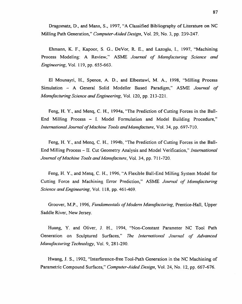
Dragomatz, D., and Mann, S., 1997, "A Classified Bibliography of Literature on NC

Milling Path Generation," Comprrler-AidedDesign, Vol. 29, No. 3, pp. 239-247.

Ehmann, K. F., Kapoor, S. G., DeVor, R. E., and Lazoglu, I., 1997, "Machining

Process Modeli ng : A Revi ew," AS ME Jozimial of Ma~nrfcrcrrrring ScÏencr and

Etz'rzeeritrg, Vol. 1 19, pp. 65 5-663.

El Mounayri, H., Spence, A- D., and Elbestawi, M. A., 1998, "Milling Process

Simulation - A General Solid Modeller Based Paradigm," ASME Journal of

Mamrfcturi~zg Science and Engineering, VoI. 120, p p. 2 1 3 -22 1 .

Feng, H. Y., and Menq, C. K., 1994% "The Prediction of Cutting Forces in the Bail-

End Milling Process - 1. Model Formulation and Model Building Procedure,"

hterrtutior~al Jozcnzal of Machirze TooO and Mamifac~zrre, Vol. 34, p p. 697-7 1 0.

Feng, H. Y., and Menq, C. H., 1994b, "The Prediction of Cutting Forces in the Ball-

End Milling Process - II. Cut Geometry Analysis and Model Verifkation," hten~atzonal

Jortnml of Mnchirze Tools und Mmrzijàcrzire, Vol. 3 4, pp. 7 1 1 -720.

Feng, H. Y., and Menq, C. K., 1996, "A Flexible Ball-End Millin; System Model for

Cutting Force and Machin ing Error Prediction," AS ME Jozirrrnl of Mnmrfnclzrrzng

Scitirtce md Engrizeering, Vol. 1 1 8, pp. 46 1-469.

Groover, M.P ., 1 996, F~mdmetrtals of Modern Marnc$octziri?ig, Prentice-Hal 1, Upper

Saddle River, New Jersey.

Huang, Y. and Oliver, J. H., 1994, "Non-Constant Parameter NC Tool Path

Generat ion on Sculptured Surfaces," T h hternationnl Jozinzal of Advanced

Ma~~zflactr~ritzg Techrzology, Vol. 9, 28 1-290.

Hwang, I. S., 1992, "Interference-fiee Tool-Path Generation in the NC Machining of

Parametrk Compound Surfaces," Comprtrr-AidedDesign, Vol. 24, No. 12, pp. 667-676.

Hwang, J. S. and Chang, Tien-Chien, 1998, "Three-axis Machining of Compound

Surfaces Using Flat and Filleted Endrnills," Compter-Aided Design, Vol. 30, No. 8, pp.

64 1-647-

Kline, W. A., DeVor, R. E., and Lindberg, J. R, 1982% "The Prediction of Cutting

Forces in End Milling with Application to Cornering Cuts," In~t.r>mntional Jozrnlal of

Machbte Tool Design alid Resrarch, Vol. 22, p p. 7-22.

Kline, W. A., DeVor, IR. E., and Shareef, 1. A., 1982b, "The Prediction of Surface

Accuracy in End Milling," ASME Journal of Etzgineeritzg for lrzdz~stiy, Vol. 104, pp.

Kline, W. A., and DeVor, R E., 1983, "The Effect of Runout on Cutting Geometry

and Forces in End Milling" Iritertzotiotznl Joz~rrzaI of Machine Toof Design ami Research,

Vd 23, pp 123-140

Lim, E. M. and Menq, C . H., 1997, "Error Compensation for Sculptured Surface

Productions by the Application of Control-Surface Strategy Using Predicted Machining

Errors," ASME Jozintal of Manrfactzu-ing Scieme mtd Erzgriieer-ing, Vol. 1 1 9, p p. 402-

409.

Lim. E. M., Menq, C. H., 1997, "Integrated Planning for Precision Machining of

Complex Surfaces. Part 1: Cutting-Path and Feedrate Optimization," International

Jor~n~alofMachbzr TooisctrzdMmrf~ctz~re, Vol. 37, No. 1, pp. 61-75.

Lim, E. M., Menq, C. H., and Yen, D. W., 1997, "Integrated Planning for Precision

Machining of Complex Surfaces. Part 2: Application to the Machining of a Turbine Blade

Die," Intenmtiorzal Jotrrtznl of Mnchitze Tools arrd Manzqlac~trre, Vol. 37, No. 1, pp. 77-

91.

Lin, R. S. and Koren, Y., 1996, "Efficient Tool-Path Planning for Machining Free-

Form Surfaces," Jorrrttal of Ertgitnerritzg for I>ldtcsîry, Vol. 1 1 8, pp. 20-28.

MarshallT S. and Griffiths, J. G., 1994, "A New Cutter-Path Topology for Milling

Machines," Compter-AidrdDesign, Vol. 26, No. 3, pp. 204-2 14.

Melkote, S. N., and Endres, W. J., 1998, "The Importance of Including Size Effect

When Modeling S lot Milli ng," AS ME Jozirnai of Ma~n&ctzir@ Scietjce md

Engiheering, Vol. 120, pp. 68-75.

Nakayama, K., and Tamura, K., 1968, "Size Effect in Metal-Cutting Force," ASME

Jozmal of Etzginerring for Zndzisby, Vol. 90, pp. 1 19-126.

Park, S., Jun, Y. T., Lee, C . W., and Yang, M. Y., 1993, "Determinhg the Cutting

Conditions for Sculptured Surface Machining," The Irt~ertintiottnl Jorcrtiol of Advanceci

Mantrfactzrri,zg Technology, Vol. 8, pp. 6 1-70.

Sim. C.. and Yane - M.. 1993. "The Prediction of the Cutting Force in Ball-End , Mi lling with a Flexible Cutter," Ititerttatiot~al Jozrrrral of M~ichine Tools and

Manzflactzrre, Vol. 3 3, pp. 267-284.

Smith, S., and Tlusty, J., 1991, "An Overview of Modeling and Simulation of the

Milling Process," ASME Jozinml of Ettgirteerittg for Indzisîry, Vol. 1 13, pp. 169-1 75.

Society of Manufacturing Engineers, 1983, Tool md Mmufuc~wittg Etzgineers

Hatdbook. Vol. 1: Machitling, Fourth Edition, Dearbom, Michigan.

Suh, Y. S., and Lee, K., 1990, "NC Milling Tool Path Generation for Arbitrasr

Pockets Defined by Sculptured Surfaces," Compzlter-Aided Design, Vol. 22, No. 5, pp.

273 -284.

Suresh, K. and Yang, D. C. H., 1994, "Constant Scallop-height Machining of Free-

form Surfaces," Joicrnal of Et,gi,irerit1g for It1dzcs&y, Vol. 1 16, pp. 253-259.

Sutherland, J. W., and DeVor, R. E., 1986, " An improved Method for Cutting Force

and Surface Error Prediction in Flexible End Milling Systems," ASME Jo11maI of

Etzgi>zeeritg for hdzrstry, Vo 1. 1 08, p p. 269-279.

Veeramani, D., and Gau, Y. -S., 1998, "ModeIs for TooI-Path Plan Optirnization in

Patch-by-Patch Mac hining," it~tentatiotml Joirnid of P roul<ctiott Resrarch, V o 1. 3 6 , No.

6, pp. 1633-1651-

Wang, J.-J. J., and Liang, S. Y., 1996, "Chip Load Kinematics in Milling with Radial

Cutter Runout," ASME Jozlnlal of Engineeritrg for I'd~~stry, Vol. 1 1 8, pp. 1 1 1 - 1 16.

Yang, M., and Park, H., 199 1, "The Prediction of Cutting Force in Ball-End Milling,"

Intert~nliotrnl J o z of Muchit~e Tools nrrd Mmnrfn~zrre, Vo 1. 3 1, p p. 45-54.

Yellowlev, 1.. 1985, "Observations on the Mean Values of Forces. Torque and

Specific Power in the Perip heral Milling Process," it~~rrtrationd Jow-td of Machine Tooi

Desigr md Research, Vol. 25, pp. 3 37-346.

Yucesan, G., and Altintas, Y., 1996, "Prediction of Bal1 End Milling Forces," ASME

Jmirnal of Etigzizeeritg for Ittdustty, Vol. 1 1 8, pp. 95- 1 03.

Zheng, L., and Liang, S. Y., 1997, "Identification of Cutter Axis Tilt in End Milling,"

ASME Jozrrnal of Mamfuctzii-itg Scietice ntrd Etgirieenng, Vol. 1 1 9, pp. 1 78- 1 8 5 .

Zheng, L., Liang, S. Y., and Melkote, S. N., 1998, "Angle Domain Analytical Model

for End Mill i ng Forces," ASME Jozrnzal of tvlanzrfac~zrritzg Science and Engheeritg

Vol. 120, pp. 252-258.