Customer order flow, information and liquidity

on the Hungarian foreign exchange market

Áron Gereben

György Gyomai

Norbert Kiss M. ♥♣

First draft: December 2005.

This version: April 2006

Abstract Customer order flow – signed transaction volume between market makers and their customers – is a key concept in the microstructure approach to exchange rates. We attempt to explore what the data tells us about the role of customer order flow in the market for Hungarian forint, using the standard analytical framework of the FX microstructure literature. Our results confirm that customer order flow helps to explain exchange rate fluctuations, which suggests that customer order flow is a key source of information for the market makers. We also find that domestic and foreign customers play significantly different roles on the euro/Hungarian forint market: foreign players’ order flow seems to provide the information that drives exchange rate fluctuations, whereas domestic customers are the source of market liquidity. We present evidence suggesting that current order flow from customers is able to provide a better forecast for the future value of the exchange rate than the ‘benchmark’ random walk model. Finally, we highlight some features of our data that suggest that beyond microstructure, the traditional portfolio-balance channel of exchange rate determination is also in place.

JEL: F31, G15

Keywords: customer order flow, microstructure, exchange rate

♥ Áron Gereben and Norbert Kiss M. are with the Department of Financial Analysis of the Magyar Nemzeti Bank (the central bank of Hungary, MNB). At the time of writing, György Gyomai was with the Department of Financial Analysis of the MNB; now he is with the OECD Statistics Directorate. Please address correspondence to Áron Gereben, Magyar Nemzeti Bank, 1850 Budapest, Hungary; email: gerebena@mnb.hu. The authors wish to thank Gyula Barabás, Csaba Csávás, Gergely Kóczán, Zsolt Kondrát, Róbert Rékási, György Sándor and Sándor Valkovszky for the comments on earlier versions of this paper. All remaining errors are ours. ♣ The views expressed here are those of the authors and do not necessarily reflect the official view of the central bank of Hungary (Magyar Nemzeti Bank).

1

1. Introduction

Customer order flow – signed transaction volume between market makers and their customers – is a key concept in the microstructure approach to exchange rates. Microstructure models, such as Kyle (1985), highlight that market-makers can extract private beliefs and knowledge about the future value of the exchange rate from customer trades, and then translate these into price changes. Customer order flow can therefore, on one hand, be a source of information. Other models, such as Evans and Lyons (2002), emphasize that once an appropriate risk premium is offered, customers are also willing to take over accumulated trading exposures from market makers. It is also an empirical fact that market makers generally close their positions at the end of each trading day. If this is true for the market as a whole, then it is the customers who must absorb the accumulated trading imbalances. Customer order flow thus can also be regarded as the ultimate source of market liquidity. This paper is mainly empirical in nature. We examine what the data tells us about the role of customer order flow in the market for Hungarian forint (EUR/HUF). Using the standard analytical framework of the FX microstructure – based on Evans and Lyons (2002) and the subsequent literature1 –, we test whether customer order flow helps explaining exchange rate fluctuations. We also identify the typical market roles of different customer types. Finally, we analyse whether current order flow from customers helps to forecast the future value of the exchange rate.

The motivation behind this study is twofold. Firstly, analysing the link between order flows and exchange rate behaviour is relevant for the practice of monetary policy, especially for countries like Hungary, who plan to join the ERM II exchange rate regime at some point, and might use, under certain circumstances, foreign exchange intervention to keep the exchange rate within the prescribed band. Knowledge on the nature and the impact of order flows may be the key to the success of these operations. Secondly, we wish to examine whether previous results, obtained using data on major currency pairs, can be extended to an emerging market’s currency. To our knowledge, this is the first study of the customer order flow – exchange rate relationship on CEEC currencies. The relatively unique database collected by the central bank of Hungary is particularly suited for such an analysis.

The relation between customer order flow and exchange rates was first examined by the pioneering works of Rime (2000), Fan and Lyons (2002) and Froot and Ramadorai (2002). The key findings of these studies are that a) customer order flow dynamics can explain the movements in exchange rates at various frequencies, and b) order flows from different customer types usually behave quite differently from each other.

More recently, a few papers explicitly examined the different behaviour of order flows from different customers. Carpenter and Wang (2003), for example, analyse spot FX transaction data from a major Australian bank. They find that order flow from the central bank and financial institutions has a positive impact on the exchange rate, whereas non-financial customers’ order flow has no influence on it. They suggest that trades with financial institutions carry more information. Mende and Menkhoff (2003), using data from

1 For a recent survey of the microstructure approach to exchange rates, see Gereben, Gyomai and Kiss M. (2005).

2

a medium-sized German bank, carried out a similar exercise and found that financial customers’ order flow is positively related to the exchange rate, whereas commercial customers’ flows are negatively related to it, i.e. commercial customers’ currency purchases coincide with depreciations.

Marsh and O’Rourke (2005) find similar results on a larger dataset, obtained from a commercial bank with a significant role on the global FX market. They argue that the difference in the impact of separate customer types’ order flow on the exchange rate suggests that the relationship between exchange rates and order flow is due to the information content of order flow, as sugggested by the information-based models of FX microstructure, rather than to the dealers’ inventory management and risk preferences, as suggested by the inventory-based microstructure theory. They argue that the inventory model would generate price reactions of same direction and magnitude across all types of order flows, no matter what type of customers are on the other side of the trade.

Probably the most detailed discussion of the relationship between exchange rates and customer order flows is by Bjønnes, Rime and Solheim (2004). They use a large and unique data-set, representing customer trades by all market-making banks on the Swedish kronor/euro market. Their starting point is the observation that market-makers generally close their positions at the end of the day, therefore there should be someone else among their customers who mops up their accumulated intraday trades. The aim of their work is to examine who – which customer group – is this longer-term liquidity provider is.

Two particularities of this study has to be pointed out. Firstly, instead of using some ad hoc specification, Bjønnes et al. derive their estimated equations from Evans and Lyons’ “workhorse” theoretical model for the FX market. Secondly, they use a cointegration framework, instead of estimating regressions between daily changes, as it is most common in the literature.

The main finding of their empirical analysis – besides confirming the dichotomy between the impact of financial vs. non-financial customers’ order flow – is that financial customers’ order flow precedes – Granger-causes – non-financial customers’ order flow. From the facts that non-financial customers’ order flow is negatively correlated with the value of the currency, and that they passively match financial customers’ order flow, the authors assert that non-financial customers are the ultimate source of liquidity on the FX market.

Yet another aspect of customer order flow, namely its potential to forecast future exchange rate movements, has been examined recently by Evans and Lyons (2005). They find that customer order flow can help predicting future changes in the exchange rate: their order flow-based forecasts were able to outperform the random walk benchmark at different forecast horizons ranging from 5 days to 1 month.

Our key results can be summarised as follows. We found a strong and significant positive relationship between a well-defined customer group’s order flow and changes in the exchange rate at a daily frequency, whereas a negative relationship was found between another customer group’s order flow and the exchange rate. This partly confirms the results obtained previously in the literature.

However, unlike in other studies, in our case it is not the financial customer vs. non-financial customer distinction that matters. Rather, the grouping is by country of origin: foreign customers’ order flow has a strong positive impact on the exchange rate, suggesting that it contains information on the future level of the exchange rate. The same is true for the central bank, although with some important qualifications. Other domestic customers,

3

on the other hand, seem to play the role of liquidity provider, as their order flow is negatively related to the exchange rate.

We also examined whether our customer order flow indicator is able to forecast the changes in the exchange rate. We found that order flow-based regressions provide forecasts with significantly lower mean squared errors than the random walk forecasts we used as a benchmark.

Looking at the data, however, revealed some puzzling features as well. Some of these suggest that beyond the microstructure effects, a portfolio-balance channel also plays a role in shaping the level of the Hungarian forint’s exchange rate. Future research is needed, however, to confirm these claims with stronger evidence. Another interesting finding is related to central bank intervention: it seems that central bank were highly succesful during times of market turmoil, but its FX transactions during normal times had no measurable impact on the exchange rate.

The paper proceeds as follows. Section 2 briefly discusses the role of customer order flow in FX microstructure theory, and provides some simple theoretical foundation to the equations estimated subsequently. Section 3 discusses the data set. Section 4 presents our estimations of the relationship between the exchange rate and customer order flow. Section 5 examines the ability of our order flow measures to forecast changes in the exchange rate. Section 6 highlights some features of the data that we could not explain using the standard FX microstructure framework. Section 7 concludes.

2. Background

In the next few paragraphs we will briefly describe the logic behind the regressions we use in the subsequent empirical analysis. As the paper’s main focus is uncover what empirics tell us, rather than to test any particular model of market microstructure, we do not provide here a rigorous and detailed theoretical model. We simply wish to show the intuition behind the equations that link the order flows of different customer groups to the exchange rate.

The equations we estimate are similar in nature to those of Bjønnes, Rime and Solheim (2004), who derive their estimated equations from the classic model of Evans and Lyons (2002).2 The intuition in our paper to link the theoretical models with empirics is quite similar to the one used by these authors. Furthermore, we also believe that the estimated equations can also be interpreted in the flavour of Kyle’s (1985) asymmetric information model. Thus we present this alternative interpretation, too.

In the classic framework of Evans and Lyons (2002), the foreign exchange trading is modelled as a three-stage process. In the first stage, the group of market makers, or dealers, receive customer orders, and thus learn about the (local) currency demand of their own customers. In the second stage of the trading, market makers trade with each other on the inter-dealer market. During this process – which is sometimes referred to as “hot potato trading” – the market plays an information aggregating-role; trading with other market makers reveals the net global demand of the whole market. Since the dealers are modelled as risk-averse participants, they wish to end the trading with a zero net open position. They

2 There is a key difference however: Bjønnes, Rime and Solheim (2004) use cointegration techniques, while we use regression on differences. However, our underlying economic interpretation is similar to theirs.

4

have to pass these positions therefore to their customers, who are also risk-averse, but they have larger risk-bearing capacity because of their size. To achieve that, market makers have to set their price in the third round of the trading in a way that it includes just the right amount of discount or premium for customers to absorb the net open positions.

This model was originally developed to explain the relationship between the exchange rate and the aggregated inter-dealer order flow, as shown in Evans and Lyons (2002). Despite the fact that in the model clear-cut relationships exist between the different types of order flows – i. e. the interdealer order flow is proportional to the first-stage customer order flow – applying the model to customer data is not trivial.

To modify the model for customer order flow, one could use the linear relationships between first-stage customer order flow and interdealer order flow and estimate an equation directly between first-stage customer order flow and the exchange rate. The problem here is how to identify the empirical, real world equivalents of the first-stage and third-stage customer trades of the Evans-Lyons model, which is necessary to calculate an empirical measure of first-stage order flow. Otherwise, if we simply aggregate across the first and third stage flows, the flows will cancel each other, and will have no relevance in an empirical model.

The property that market-wide customer order flows aggregated over a trading day cancel each other out is not an ad hoc property of the Evans-Lyons framework. It has been often observed that market makers, in general, close trading days with no or very small open positions (see, for example, Bjønnes and Rime, 2003). A consequence of this is that net bank-wide or market-wide aggregate customer order flow should only randomly be different from zero, and it should not be correlated with the exchange rate.

Some studies, for example Fan and Lyons (2002), use fully aggregated customer order flows, and find that it, despite all the above, can explain exchange rate fluctuations. A potential explanation for this result is that these studies use order flow data from a single market maker, and this market maker’s clients order flow does not necessarily represent the market-wide customer order flow. For instance, it can happen that the clients of certain large market makers are more informed than the typical client on the market. In the aggregate customer order flow of such market-makers the trades from the well-informed, ‘high-impact’ customers are overrepresented, and thus it actually may help to explain the exchange rate.

Another approach is to assume that different customer types act as counterparties in the different stages of the trading process. Once we can identify who are the typical first-round customers, and who are the ones usually in the third-round, we can create separate “first-round” and “third-round” customer order flow aggregates, and use them in regressions explaining changes in the exchange rate. Estimated equations in studies, such as Carpenter and Wang (2003), Mende and Menkhoff (2003), Marsh and O’Rourke (2005) and Evans and Lyons (2005), that use disaggregated customer order flows, can be interpreted in this manner.

Bjønnes, Rime and Solheim (2004) make this interpretation explicit. They estimate customer order flow models based on the Evans-Lyons model, augmented with assumptions described above: i.e. that separate customer segments participate in the first and third stages of trading. Besides giving an interpretation of the link between exchange rates and customer order flow within the Evans and Lyons framework, they introduce the notion of “push customers” and “pull customers”. Push customers are the first-round customers: they tend to move to the market, initiate orders and cause price changes. Pull

5

customers are the third-round customers: they are attracted to the market by price changes and they considered to possess no private information about the value of the currency. They may be driven to the market by random liquidity needs, but they can time their entry and wait for a good price. They absorb the shocks caused by the push customers by providing liquidity, and their order flow is likely to be correlated negatively with the exchange rate.

We suggest a complementary interpretation of the relationship between different customer order flow aggregates and the exchange rate using the information-based logic of Kyle (1985). In the stylized world of Kyle’s model there exists an uninformed market maker who receives a flow of informed and uninformed orders that are undistingusihable from each other. The market maker is characterized by two distinctive features: she adjusts prices to protect herself against information-based trades, and she provides the necessary liquidity for the market.

On the foreign exchange market, no single candidate on the market has both these characteristics. However, we can consider the dealers and the pull-customers together as a joint entity that comes close to Kyle’s concept of the market maker. The dealers master the technique of price setting, but provide liquidity for only a very short time; whereas the pull-customers are willing to take over the positions accumulated from the actions of the push-customers. Using this approach, the Kyle model and its implications are thus valid for what we called the first-round trading – or trading with push customers – previously. In this interpretation, public information is the driver behind the positive relationship between the first-round customer order flow and the exchange rate. The order flow of the non-informed liquidity providers, who take over the accumulated positions from the market makers, will correlate negatively with the exchange rate.

3. Data and summary statistics

Our data set contains forint/euro exchange rates and the corresponding customer order flow data at daily frequency. It covers almost four years (from 7 November 2001 to 3 October 2005) and a total of 980 observations. Data are compiled from two data sources.

The exchange rate data contains quotes from the Reuters D2000 trading system. We used the midpoint of the best bid and ask quotes at 5.00PM each day, and used the logarithmic difference to create a series of daily log changes of the exchange rate. The heavy trading hours finish by 5:00 p.m., therefore we can assume that we can capture the daily exchange rate movements related to the order flow of a given day.

The source of order flow data is the Daily Foreign Exchange Report of the Magyar Nemzeti Bank (MNB, the central bank of Hungary), which contains all foreign exchange transactions of significant size carried out by commercial banks residing in Hungary. This data allows us to calculate daily order flow measures between domestic market-making banks and different customer groups.

As we do not know the initiator of the single trades, we made an assumption that is wide-spread in the customer order flow literature, namely that trades between market makers and customers are always initiated by the customer side. We used this assumption as a guideline to determine trade sign, and calculated the order flows accordingly. More details on the database and the process of transforming raw data into order flow measures is in Appendix 1.

6

Our time span is relatively long by the standards of the FX microstructure literature. The data set contains both spot and forward market order flows, and we treat those as separate variables.3

The coverage of our order flow data set is not complete. The data covers only domestic commercial banks, as financial institutions registered outside Hungary do not have reporting obligations to the MNB. As a result, the database gives a partial picture of the forint/euro market, as some market makers are located offshore. We do not have precise information about the size of the offshore forint/euro market. Anecdotal evidence indicates that the offshore turnover is significant; however, the most important market makers are said to be the locally based ones.

This feature puts our database, in terms of coverage, halfway between the two approaches generally used in empirical analyses of customer order flow. Our data provides us with a more complete picture of the given market than the one in those studies that use data from a single market-maker (e.g. Fan and Lyons, 2002; Froot and Ramadorai, 2002; Carpenter and Wang, 2003; Mende and Menkhoff, 2003; Marsh and O’Rourke, 2005). However, it does not provide the full picture of the market, such as the data in Rime (2000) and Bjønnes, Rime and Solheim (2004), which, at least theoretically, cover all significant trades of the observed markets.

The database contains information on counterparty identity. This allowed us to distinguish the domestic market-makers’ order flows with the following counterparty types:

• domestic (non-marketmaking) banks; • domestic non-banks; • the central bank; • foreign banks; • and foreign non-banks.4

These order flow measures has been calculated for both the spot and the forward market transactions.

The Hungarian forint’s exchange rate is allowed to fluctuate within a +/- 15 per cent band relative to the euro. For most of the period, the exchange rate was floating within this wide band. However, in January 2003, it reached the strong edge of the band and stayed there for two days, while the central bank was carrying out large-scale interventions. As to the size of the market, the domestic market makers’ average daily spot market turnover amounted to about 400 million euro during the time period considered, while the forward market’s average turnover was around 50 million euro.

Tables and charts with descriptive statistics of the data can be found in Appendix 2. Looking at the turnover data by customer types (see Table A1 in Appendix 2), it seems that about half of the domestic market makers’ trading is with foreign banks, while domestic

3 Most studies of customer order flow use spot market data only. One exception is Bjønnes, Rime and Solheim (2004), who aggregate spot and forward trades into a single combined order flow variable. 4 Unfortunately, the data does not allow us to further separate the non-bank categories into financial and non-financial customers, a distinction that has proven to be of interest in most of the earlier studies. Such a breakdown is only possible for the data in 2005, and only for the domestic non-bank series.

7

banks and non-bank customers are also heavily represented.5 Foreign non-bank customers play a relatively insignificant role on the market in terms of turnover.6

It is worthwhile to look at the correlations between the different order flows, as it can give us a preliminary hints on the roles of different customer types (see Table A2 in Appendix 2). One interesting feature is that none of the single order flow variables show correlation with the exchange rate. Some order flow indicators, however, show strong correlations with each other. It can be noted that, in general, correlation between domestic and foreign participants’ order flow is negative. This suggests that they may play opposite roles on the market, i.e. being ”push customers” and „pull customers”.

Our sample is heterogenous in a sense that it contains periods when the Hungarian foreign exchange was relatively calm, and periods of high turbulence as well. This heterogeneity plays an important role in our subsequent empirical analysis, especially when we look at the stability of the results. Besides using the whole sample, we will also examine whether our results hold for certain periods with unique characteristics. For this purpose, we will divide our sample into three subsamples: (i) from 7 November 2001 to 31 December 2002; (ii) from 1 January 2003 to 31 December 2003; and (iii) from 1 January 2004 to 3 October 2005.

Some background information on these subperiods may be useful for the further analysis. The first subperiod was relatively calm. The forint’s exchange rate stayed near the strong edge of its fluctuation band (see Chart A3 in Appendix 2), and in most of the time fluctuated within a narrow range, between 240 and 250. The order flow data is also characterised with relatively low variance (see Table A4 in Appendix 2). The database does not show any central bank FX operations being carried out during this period.

The year of 2003 can be characterized as a turbulent period. Extraordinary events – such as a speculative attack against the strong edge of the forint’s fluctuation band, a devaluation of the band’s central parity, sudden large shifts in the central bank’s key policy rate etc. – contributed to an increase in exchange rate volatility. Large daily depreciations happened in more than one occasion. The disorderly market conditions were reflected in the order flow as well. Variances of the spot market order flow measures are significantly higher than in any other periods. The central bank’s market activity was important during this period.

One event of this period which is particularly noteworthy is the speculative attack against the strong edge of the fluctuation band, which happened in January. During this time, the central bank intervened not only through the usual domestic market makers, but executed trades in considerable amount with domestic non-marketmaking banks as well. As trades between non-marketmaking entities are usually not considered to be important enough in size to be relevant for price determination, this intervention does not show up in our order flow measures. However, in this particular case, the order flow between non-dealer banks and the MNB was important, and it was necessary to add this particular order flow to some

5 The large amount of trading that occurs with foreign banks may reflect a certain weakness of our data set, namely that we cannot distinguish between foreign-based market-makers and other foreign banks. As a result, a large part of the order flow we assign to foreign bank customers may be a result of inter-dealer trading, rather than pure customer trading. A more detailed discussion of this problem can be found in Appendix 1. 6 Part of the foreign banks’ order flow may represent indirect trades by non-bank customers, thus the role of foreign non-bank entities on the euro/forint market is likely to be much larger than this data suggests. However, our database do not allow to distinguish between foreign banks’ proprietary trades and customer orders.

8

of the regressions as an auxiliary variable. It takes up positive values only during the two days of the speculative attack, and is zero otherwise.

In the last period the exchange rate followed a slow appreciating trend. Once again it was a relatively calm period, with the exchange rate volatility reverting back to normal levels. Order flow data is similar: the standard deviations are smaller relative to the year 2003. The central bank appeared on the market from time to time, but its role was much more subdued than in the preceding subsample.

4. Econometric analysis

In this section we use empirical analysis to explore the relationships between customer order flows and the exchange rate. Firstly, we examine the links between spot market order flows and the exchange rate. Secondly, we extend the analysis to forward order flows as well. Finally, we look at the (temporal) stability of our results.

Spot market order flow. We begin our empirical analysis by estimating two versions of the order flow model. In both versions we attempt to explain daily exchange rate dynamics with spot market order flows. In the first, generic version of the model we include all order flow variables in a single equation, without separating the order flows from push and pull customers.7 For the second model, we estimate two equations, which, in the spirit of Bjønnes, Rime and Solheim (2004) treat the order flows originating from push and pull customers separately.

The generic model takes the following form:

ti

itit xds εββ ++= ∑0 , { }cbdodbfofbi ,,,,= (1)

where dst is the logarithmic daily change in the exchange rate, and xit are the different

components of the market makers’ daily spot customer order flow, namely the order flow from foreign banks (xfb

t), foreign non-bank entities (xfot), domestic non-marketmaking

banks (xdbt), domestic non-bank entities (xdo

t), and the central bank (xcbt).8 Order flows are

measuerd in billion forints. After testing the residuals of our preliminary estimates, we found evidence of autoregressive conditional heteroskedasticity, thus we imposed a GARCH (2, 1) structure on the model’s variance.

We estimate the generic model at daily frequency for the full sample using maximum likelihood. The results show that the estimated coefficients of the foreign banks’, foreign non-banks’ and central bank’s order flows are highly significant (see column 1 in Table 1). The negative sign of these coefficients suggest that HUF purchases by these types of customers generally result in an appreciation of the Hungarian currency relative to the 7 We use the notions of push customers and pull customers in the sense described in Section 2. To recapitulate, push customers’ buy orders coincide with appreciations of the currency; these customers are understood to provide the market with information that is not yet common knowledge through their trades. Such trades are also considered to drive exchange rate dynamics. Pull customers’ purchases coincide with currency depreciation, and they are assumed to provide liquidity to the market. 8 As it was discussed in the previous section, during the two days of the speculative attack against the forint some non-marketmaking domestic banks carried out direct trades with the central bank. We included these trades as an auxiliary variable in those regressions that include the order flows from domestic banks. The inclusion of this information in the regressions helped us to increase parameter stability. Replacing this auxiliary variable with a speculative attack dummy yields similar results.

9

euro.9 The foreign-based trading partners, together with the central bank, could therefore be considered as push customers. The coefficients of the domestic banks and non-banks are not significantly different from zero.

The overall fit of the model is relatively high: the adjusted R2 of approximately 30 per cent is of the same magnitude as reported in similar studies in FX microstructure literature. The diagnostics do not suggest autocorrelation or heteroskedasticity over and above the imposed GARCH structure.

In the case of the specific model we followed the footsteps of Bjønnes, Rime and Solheim (2004) and distinguished between “push” and “pull” customers by running separate regressions for the two groups.

We assigned the role of push customers to foreign participants and the central bank, and let domestic banks and non-bank customers play the role of pull customers. This choice was partly motivated by the correlation analysis of the order flows, described in section 3, and partly by the results of the generic model, which suggested the candidates for being the push customers.

We estimated Equation 1 separately for the two groups, i.e. using i={fb, fo, cb} and i={db, do}.10 Besides the explanatory variables the regression specifications were the same. The results are in columns 2 and 3 in Table 1.

The push customer equation yields results that are similar to the generic version of the model. Coefficients attributed to the order flows of the foreign customers and of the central bank are highly significant. The adjusted R2 indicates an explanatory power similar to the generic model. This suggests that order flows originating from foreign customers – together with the flow from the central bank – are the key drivers of exchange rate fluctuations.

It is also interesting to look at the regression with the pull customers. Once being put into a separate equation, the order flow coefficients of the domestic banks and domestic non-banks become highly significant. The sign of the coefficients is positive, which indicates that domestic customers’ forint purchases generally coincide with a depreciation of the Hungarian currency. The explanatory power of the equation is lower than the one with the push customers. The regression diagnostics are satisfactory.

9 The usual quotation of the currency pair is HUF/EUR, therefore an increase in the exchange rate corresponds to a depreciation of the forint. Negative coefficients for the order flow hence indicate buy orders making the forint to appreciate, while positive coefficients indicate a depreciating impact. 10 Bjønnes, Rime and Solheim (2004) use co-integration technique and include an error correction term in their model. Their specification implicitly suggests an equilibrium relationship between the exchange rate and cumulated order flows, where deviations from this equilibrium level tends to diminish over time. In our view this error correction mechanism is not necessarily an integral part of the underlying microstructure theory, therefore we carried out the estimations in terms of differences.

10

Table 1.: Spot market order flow and exchange rate dynamics – estimation results*

Variables

(1)

Generic model

(2)

Model with push customers

(3)

Model with pull customers

Constant (β0) -0.082 (-1.06)

-0.114 (-1.55)

0.058 (0.60)

Foreign banks’ order flow (βfb) -0.124 (-17.91)

-0.127 (-21.42)

-

Foreign non-banks’ order flow (βfo)

-0.186 (-12.12)

-0.201 (-14.22)

-

Domestic (non-market making) banks’ order flow (βdb)

0.027 (1.17)

- 0.285 (14.41)

Domestic non-banks order flow (βdo)

0.003 (0.24)

- 0.115 (7.28)

Central bank’s order flow (βcb) -0.185 (-11.66)

-0.169 (-28.64)

-

Order flow from dom. non-market-making banks to the central bank

-0.376 (-1.14)

- -1.299 (-19.61)

Diagnostics

Adjusted R2 0.302 0.305 0.147

P-value, serial correlation Q-test (lags: 1, 5)

0.16, 0.25 0.17, 0.23 0.50, 0.60

P–value, ARCH LM test for heteroskedasticity (lags: 1, 5)

0.84, 0.80 0.84, 0.75 0.96, 0.90

*Dependent variable: daily logarithmic change of the EUR/HUF exchange rate. Parameter z-statistics are in parentheses. Sample period: 8 Nov 2001 – 3 Oct 2005. Number of observations: 979. Estimation method: maximum likelihood.. ARCH and GARCH components are not included. To test for serial correlation, null probabilities derived from a Ljung-Box Q-test using 1 and 5 lags are shown. To test for heteroskedasticity, p-values dericved from the ARCH LM test (using F-statistics) are shown. Parameter estimates significant at a 1 per cent level are shown with bold typeface.

The observation that order flows from the domestic banks and non-banks are not significant in the generic model, but significant in the pull customer model is likely to be due to the fact that pull customers’ order flow, in approximate terms, is a mirror image of the push-side order flow. Market maker exposures arising from trades with push customers are absorbed during the day by the pull customers, who provide the liquidity. The two variables are thus conveying approximately the same information. Putting the two types of order flow in the same equation yields to multi-collinearity between the explanatory variables; which, in our case, renders the parameters of the push side non-significant.

The overall results are in line with our initial expectations. Firstly, order flows performed well in explaining exchange rate dynamics. Secondly, the estimated equations confirm that foreign entities, together with the central bank, play the role of push customers on the EURHUF market. Domestic customers, on the other hand, act as pull customers and provide liquidity to the market.

This second finding is somewhat surprising in the sense that it is not fully in line with previous research in this area. Earlier studies, such as Mende and Menkhoff (2003),

11

Bjønnes, Rime and Solheim (2004) and Marsh and O’Rourke (2005), find that it is the distinction between financial and non-financial customers’ order flow that matters for determining the sign of the order flows’ impact on the exchange rate, rather than the distinction of domestic and foreign customers.

One possible reason why in our case it is the distinction of foreign- and domestic-originating order flow that separates the push customers from the pull customers may be that our data does not allow the separation of financial and non-financial non-bank customers’ order flow. It is possible that if we could further break down our order flow variables, and create series of financial and non-financial customers’ order flow, then that specification would yield to a similar or better separation between push and pull customers.

However, from January 2005, the data allowed us to break down the domestic non-bank order flow series into financial and non-financial customers. We used these disaggregated series in regressions on the available subsample to test the importance of this effect. We did not find significant differences in the behaviour of financial and non-financial domestic customers’ order flow. Although this short sample does not allow us to draw strong conclusions, it suggests that the non-standard result may not be due to the data availability problem.

Another potential explananation stems from the fact that Hungary is an emerging market economy, relying heavily on foreign capital flows. A large share of the economic fundamentals governing the forint’s exchange rate are dependent on external factors. As a result, it is likely that foreign customers are more likely to convey non-public information about future fundamentals through their trades than domestic customers.

Forward market order flow. So far we considered only the order flow on the spot market. Our data set allows us to also include forward market order flows into the model. We re-estimated the push and pull customer models extended with the forward market variables, by customer type and nationality. Table 2 shows the push- and pull-side equations, with forward market order flows included when significant.

The inclusion of forward market order flow has not changed the overall picture in case the push-side equation. None of the forward market order flow variables have a push-type impact on the exchange rate. It seems that the primary channel that aggregates information about the future value of the currency is the spot market.

In the pull customer regression, however, domestic non-banks’ forward order flow is highly significant, and its inclusion considerably improved the R2 value of the equation, too. This suggests that the forward market plays a role in liquidity provision.11 It is interesting to note that foreign banks’ forward order flow has also been siginficant in the pull-side equation in some subperiods; however, this result has not proven to be stable over time.

11 The introduction of the forward order flow, however, resulted in the deterioration of the regression diagnostics, which suggest further autocorrelation and autoregressive heteroskedasticity over and above the imposed GARCH structure.To compensate for these factors we also estimated the model using Newey and West (1989) standard errors. The Newey-West correction resulted in somewhat higher standard errors for the parameters, but has not changed the fundamental picture.

12

Table 2.: Spot and forward market order flow and exchange rate dynamics – estimation results*

“Push”-side equation

Variables

Coefficients

“Pull”-side equation

Variables

Coefficients

Constant (β0) -0.114 (-1.55)

Constant (β0) 0.046 (0.51)

Foreign banks’ spot order flow (βfb)

-0.127 (-21.42)

Domestic non-marketmaknig banks’ spot order flow (βdb)

0.225 (9.97)

Foreign non-banks’ spot order flow (βfo)

-0.201 (-14.22)

Domestic non-banks’ spot order flow (βdo)

0.129 (6.50)

Central bank’s order flow (βcb) -0.169 (-28.64)

Domestic non-banks’ forward order flow

0.128 (10.66)

Order flow from dom. non-market-making banks to the central bank

-1.09 (-12.04)

Diagnostics Diagnostics

Adjusted R2 0.302 Adjusted R2 0.233

P-value, serial correlation Q-test (lags: 1, 5)

0.16, 0.25 P-value, serial correlation Q-test (lags: 1, 5)

0.01, 0.02

P–value, ARCH LM test for heteroskedasticity (lags: 1, 5)

0.84, 0.80 P–value, ARCH LM test for heteroskedasticity (lags: 1, 5)

0.93, 0.57

*Dependent variable: daily logarithmic change of the EUR/HUF exchange rate. Parameter z-statistics are in parentheses. Sample period: 8 Nov 2001 – 3 Oct 2005. Number of observations: 979. Estimation method: maximum likelihood.. ARCH and GARCH components are not included. To test for serial correlation, null probabilities derived from a Ljung-Box Q-test using 1 and 5 lags are shown. To test for heteroskedasticity, p-values dericved from the ARCH LM test (using F-statistics) are shown. Parameter estimates significant at a 1 per cent level are shown with bold typeface.

Stability. In section 3 we elaborated on the temporal heterogenity of the sample. Due to the differences between the sample’s sub-periods, it is thus worthwhile to examine how stable the relation between the exchange rate and order flow was over time.

To perform the stability test we estimated the “push-side” and the “pull-side” equations over two different sub-samples: the pre-2003 sample and the post-2003 sample (Table 3.). Our main goal was to examine whether the parameters were similar for the two relatively shock-free sub-periods, therefore we did not perform a separate estimation for the year 2003. We included only the “best fit” version of the models, i. e. we included only the significant variables – the cut-off probability was 5 percent – in the model, besides the constant.

The estimated regressions indicate that our overall results are relatively stable. The sign and the magnitude of the key order flow coefficients are similar in both the pre-2003 and the post-2003 sample, and they are also comparable to the full-sample results. The only notable shift is the increase in the coefficient of domestic banks’ order flow, however, the sign of the coefficient has not changed. Regression diagnostics are somewhat inferior in the first subsample than either in the post-2003 sample and in the full sample. The lower R2 indicate weaker explanatory power, and some additional serial correlation is also present. However, all in all, most of our conclusions hold for each subsample.

13

Table 3.:Stability analysis – estimation results*

“Push”-side equation

Variables

Pre-2003

Coefficients

Post-2003

Coefficients

“Pull”-side equation

Variables

Pre-2003

Coefficients

Post-2003

Coefficients

Constant (β0) -0.130 (-1.08)

-0.247 (-2.06)

Constant (β0) 0.022 (0.125)

0.057 (0.452)

Foreign banks’ spot order flow (βfb)

-0.104 (-11.07)

-0.139 (-13.77)

Domestic non-marketmaking banks’ spot order flow (βdb)

0.161 (4.957)

0.390 (7.216)

Foreign non-banks’ spot order flow (βfo)

-0.212 (-13.86)

-0.260 (-5.63)

Domestic non-banks’ spot order flow (βdo)

0.101 (2.75)

0.152 (7.025)

Central bank’s order flow (βcb)

n.a. - Domestic non-banks’ forward order flow (βdbf)

0.111 (5.50)

0.076 (3.600)

Diagnostics Diagnostics

Adjusted R2 0.259 0.326 Adjusted R2 0.110 0.217

P-value, serial correlation Q-test (lags: 1, 5)

0.01, 0.00 0.65, 0.29 P-value, serial correlation Q-test (lags: 1, 5)

0.01, 0.02 0.25, 0.13

P–value, ARCH LM test for heteroskedasticity (lags: 1, 5)

0.59, 0.62 0.86, 0.99 P–value, ARCH LM test for heteroskedasticity (lags: 1, 5)

0.71, 0.60 0.95, 0.91

*Dependent variable: daily logarithmic change of the EUR/HUF exchange rate. Parameter z-statistics are in parentheses. Sample periods are: 8 Nov 2001–31 Dec 2002 (283 obs) for pre-2003 and 5 Jan 2004–3 Oct 2005 (446 obs.) for post-2003 . Estimation method: maximum likelihood. ARCH and GARCH components are not included. To test for serial correlation, null probabilities derived from a Ljung-Box Q-test using 1 and 5 lags are shown. To test for heteroskedasticity, null probabilities dericved from the ARCH LM test (using F-statistics) are shown. Parameter estimates significant at a 1 per cent level are shown with bold typeface.

The only key exception is the central bank’s order flow, which is present with a strong and significant coefficient in the full-sample regression, and is missing from both the pre-2003 and post-2003 regressions. The central bank has not carried out any transaction with domestic market makers during the span of the first subsample, thus it is natural that its order flow does not feature in the regression. During the post-2003 sample, the central bank carried out some foreign exchange transactions with the domestic market makers, although the amounts were relatively small compared to 2003. This order flow does not have a significant exchange rate impact, if put in the post-2003 regression. The strong impact of the central bank transactions on the exchange rate measured in the full-sample regression, is hence exclusively due to the events of 2003. We provide further analysis of this finding in section 6.

We can summarize the results of the empirical analysis in the followings.

• Daily customer order flow is able to explain a significant part of the fluctuations of the forint/euro exchange rate.

• The data is consistent with the model of push and pull customers. Foreign customers and the central bank seem to play the role of push customers, while domestic clients are the pull customers. This result differs from the findings of other authors, who usually find that financial clients are the push customers, and non-financial customers are the pull ones, irrespective of their location.

• Forward market order flow is important only in the pull customers’ equation.

14

• The results are relatively stable over time, with the impact of the central banks’ transactions being the only notable exception.

5. Forecasting ability

When evaluating order flow models, the FX microstructure literature usually distinguishes between two different concepts of forecasting ability. The first concept traces back to the well-known study by Meese and Rogoff (1982), who compare the performance of different exchange rate models by looking at their out-of-sample forecasting performance relative to the random walk model. The Meese-Rogoff test, however, does not involve ‘true’ forecasting, as it uses the actual realised values of the models’ contemporaneous explanatory variables; an information that a real-life forecaster would not know. In a sense, it is more a test of out-of-sample model fit than of forecasting ability.

The Meese-Rogoff test has become a standard tool of model evaluation in the empirical exchange rate economics in general, and the empirical FX microstructure literature in particular. As it was shown in Meese and Rogoff’s original article and in the following literature, most macroeconomic models do not score particularly well in the test. They usually cannot beat the random walk, at least not on ‘forecasting’ horizons shorter than one year. Microstructure-based models, on the other hand, are often successful in producing results better than the random walk benchmark.

Besides testing forecasting ability in the Meese-Rogoff sense, there has been some attempts to test the ‘true’ forecasting ability of order flow model as well, where future changes in the exchange rate is predicted using only current and past values of the explanatory variables. A promising example is by Evans and Lyons (2005). Using customer order flow data from Citibank, they show that current-period order flow can actually predict future exchange rate changes better than the random walk model.

In this chapter we examine the forecasting performance of our customer order flow data using both the weaker (Meese-Rogoff) and stronger (true predictions) concept of forecasting ability.

To perform the forecasting exercises, we had to select two data periods: one for carrying out the estimations and one to do the forecasts. Due to the heterogenous nature of the data, we decided to focus on the post-2003 segment of the sample during the forecasting exercise. In particular, we used the period from June to December 2004 for estimating the forecasting equations, and used the remaining data of the year 2005 to perform the forecasts themselves. We have chosen five forecasting horizons: 1 day, one week (5 days), two week (10 days), one month (20 days) and three months (60 days).

Meese-Rogoff-type forecasting exercise. To carry out the Meese-Rogoff-type forecast tests, we picked the pull customer specification from the previous chapter, i. e. the equation that explains the logarithmic change of the exchange rate (dst) with the order flows from foreign banks (xfb

t) and foreign non-bank entities (xfot). Formally:

tfo

tfb

tt xxds εβββ +++= 210 . (2)

We first estimated the above equation from June to December 2004, a sample of 150 observations altogether, then re-estimated the equation in each forecast round, adding new data from the previous period to the sample. We calculated the ‘forecasts’ in each period

15

between January and September 2005 for the five different forecasting horizons using the following equation:

∑∑=

+=

++ +++=h

i

foit

h

i

fbittht xxhss

12

110 βββ , h =[1, 5, 10, 20]. (3)

We converted the log forecast values back to level forms, and compared the forecast values to the actual exchange rate data. Finally, we calculated the forecasts’ mean squared errors (MSE), and compared the order flow model’s MSE with the performance of the random walk (Table 4.).

Table 4.: Out-of-sample forecasting performance (Meese-Rogoff)

Forecast horizon (days) h=1 h=5 h=10 h=20

MSE (order flow model) 0.34 1.55 3.38 7.36

MSE (random walk) 0.55 2.52 5.67 10.90

MSE ratio (order flow/RW) 0.62 0.62 0.60 0.67

It is obvious from the table that the customer order flow model performs quite well in the Meese-Rogoff test. Depending on the forecast horizon, the model produced MSE values that are 33-40 percent smaller than the results of the random walk benchmark. Although the Meese-Rogoff test tells us little about the model’s true forecasting ability, it confirms that the out-of-sample fit of the model is relatively good.

An important finding is that the model performs relatively well, even at the longer forecast horizons. This suggests that the impact of customer order flow on the exchange rate is not a short-term, transitory phenomenon. Rather, it seems that order flow shocks cause permanent – or at least rather long-lasting – impacts on the exchange rate; long enough to be relevant for the purpose of monetary policy.

True forecasting ability. In a real forecasting exercise, however, the contemporaneous values of the explanatory variables –order flows in our case – are not known. To be able to forecast in the absence of contemporaneous explanatory variables, we have two options. Either we use the already estimated models and provide forecasts for the future values of the explanatory variables in a separate step, or we can re-estimate our models to use lagged-values of the explanatory variables.

Following Evans and Lyons (2005), we used the latter forecasting technique. We estimated a regression model in which we explained contemporaneous changes in the exchange rate with past order flows at different time horizons. The sample covered June - December 2005. Then we used these equations to forecast exchange rate changes in the remaining part of the sample (the year 2005), with re-estimating the regression in every forecasting round, incorporating the new data as it became available. 12

12 One obvious question that arises here is whether microstructure theory suggests any non-contemporaneous relationship between aggregate order flows and the exchange rate. In other words, do we have theoretical grounds to propose that today’s aggregate order flow could explain the exchange rate in the future. Evans and Lyons (2005) argue that a lagged impact of the aggregate order flow could be attributed to the fact that market makers cannot observe the aggregate order flow. They observe the order flow from their own customers. The order flow at the market’s level reveals itself slowly during the inter-dealer trading process. This may explain delays between order flow shocks and their impact to the exchange rate.

16

For comparability, we used the same explanatory variables as in the models we used in the Meese-Rogoff exercise. We also covered the same sample period.

Specifically, our forecasting relationship was inferred from the following model:

∑∑∑=

+=

−=

−+ +++=−h

iit

h

i

foit

h

i

fbittht xxss

102

010 εβββ , h =[1, 5, 10, 20] (4)

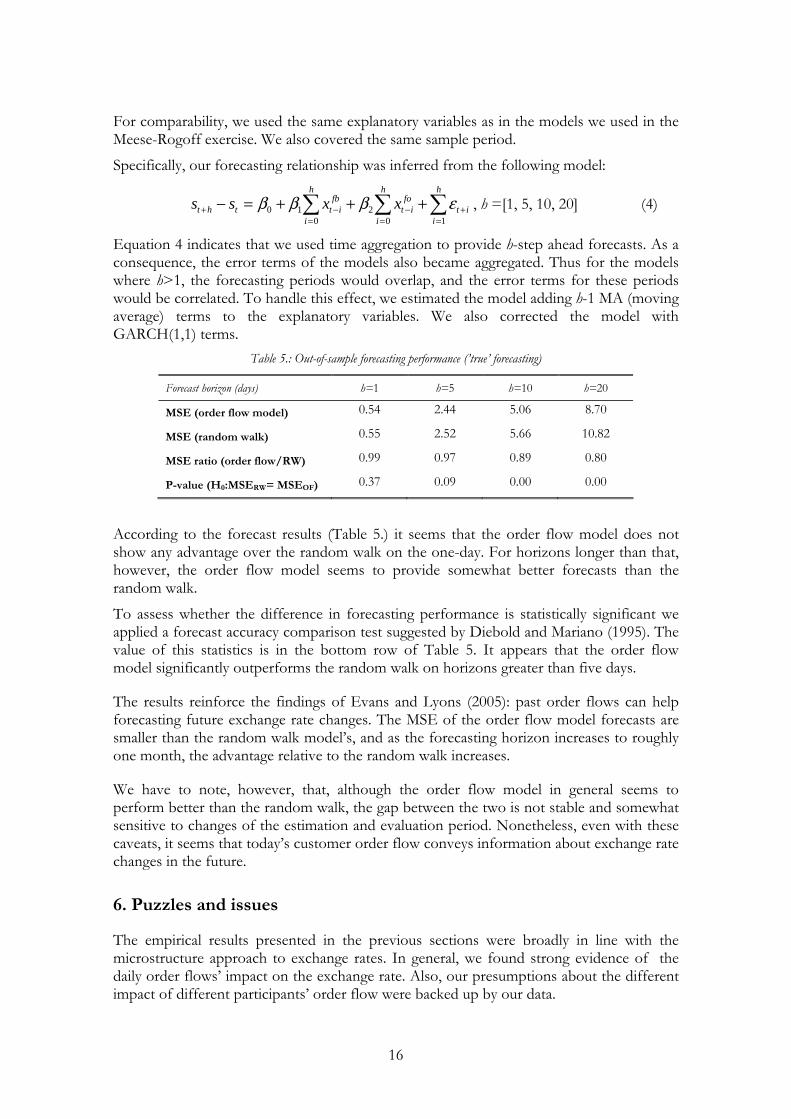
Equation 4 indicates that we used time aggregation to provide h-step ahead forecasts. As a consequence, the error terms of the models also became aggregated. Thus for the models where h>1, the forecasting periods would overlap, and the error terms for these periods would be correlated. To handle this effect, we estimated the model adding h-1 MA (moving average) terms to the explanatory variables. We also corrected the model with GARCH(1,1) terms.

Table 5.: Out-of-sample forecasting performance (’true’ forecasting)

Forecast horizon (days) h=1 h=5 h=10 h=20

MSE (order flow model) 0.54 2.44 5.06 8.70

MSE (random walk) 0.55 2.52 5.66 10.82

MSE ratio (order flow/RW) 0.99 0.97 0.89 0.80

P-value (H0:MSERW= MSEOF) 0.37 0.09 0.00 0.00

According to the forecast results (Table 5.) it seems that the order flow model does not show any advantage over the random walk on the one-day. For horizons longer than that, however, the order flow model seems to provide somewhat better forecasts than the random walk.

To assess whether the difference in forecasting performance is statistically significant we applied a forecast accuracy comparison test suggested by Diebold and Mariano (1995). The value of this statistics is in the bottom row of Table 5. It appears that the order flow model significantly outperforms the random walk on horizons greater than five days.

The results reinforce the findings of Evans and Lyons (2005): past order flows can help forecasting future exchange rate changes. The MSE of the order flow model forecasts are smaller than the random walk model’s, and as the forecasting horizon increases to roughly one month, the advantage relative to the random walk increases.

We have to note, however, that, although the order flow model in general seems to perform better than the random walk, the gap between the two is not stable and somewhat sensitive to changes of the estimation and evaluation period. Nonetheless, even with these caveats, it seems that today’s customer order flow conveys information about exchange rate changes in the future.

6. Puzzles and issues

The empirical results presented in the previous sections were broadly in line with the microstructure approach to exchange rates. In general, we found strong evidence of the daily order flows’ impact on the exchange rate. Also, our presumptions about the different impact of different participants’ order flow were backed up by our data.

17

However, the analysis of our data revealed some additional features that we were either unable to explain through microstructure theory, or they are somewhat in odds with other research in this area.

In this subsection we will elaborate on these „puzzles”. We would like to emphasise that our aim here is to highlight some empirical observations and speculate about potential underlying causes in order to generate further discussion, rather than providing a definite explanation.

The first puzzle we discuss is an observed relationship between the exchange rate and some stock quantity variables. As we have seen in the previous sections, strong relationship exists between the exchange rate changes and order flows. This is in line with microstructure theory. However, it is apparent from the data that co-movements exist between the level of the exchange rate and some stock variables, too. The variable that shows a particularly strong long-term co-movement with the exchange rate, indicating the possibility of co-integrating relationship, is the forward market position of domestic non-bank customers. The two variables are plotted on Chart 1.13

From the chart it seems that there exist a relationship not only between the daily changes, but also between the levels as well, as far as the non-banks’ forward stock is concerned. Moreover, this forward stock variable is not a simple cumulative order flow measure. Besides the new forward transactions executed a certain day – from which order flow can be calculated –, it also contains stock changes due to the expiry of forward contracts, too. (The simple cumulated order flow measure does not show such a strong relationship with the exchange rate).

If we believe that the impact of order flow to the exchange rate is mainly due to its information content, it is difficult to explain why the expiry of forward contract should make a difference in terms of the level of exchange rate. Forward expiries do not seem to reveal any new, not yet publicly known information that could rationalise its impact on the exchange rate.

One potential explanation is that, beyond the microstructure effects, portfolio-balance effects also play a role in exchange rate determination. The portfolio-balance approach assumes that assets denominated in domestic and foreign currencies are not perfect substitutes. Investors are assumed to be risk-averse and to hold domestic and foreign assets to diversify risk. The composition of their portfolio is determined by different sources of risk connected to these assets. Therefore they expect compensation for portfolio shifts in the form of higher relative relative rate of returns. In such cases exchange rate can be affected by portfolio-realignments, like forward expiries.

13 The Johanssen test confirms the existence of a long-run relationship at 5% significance level (see Appendix 2. Table AA4.).

18

Chart 1: Exchange rate and domestic non-banks' forward stock

-100

-50

0

50

100

150

200

250

300

350

400

450

500

550

600

Jan/

2004 Fe

b

Mar

Mar

Apr

May Jun

Jul

Aug Sep

Oct

Nov Dec

Jan/

2005 Fe

b

Mar

Apr

May Jun

Jun

Jul

Aug Sep

billion forint237,5

240

242,5

245

247,5

250

252,5

255

257,5

260

262,5

265

267,5

270

272,5

HUF/EUR

domestic non-banks' forward stock exchange rate The second issue is the relationship between the Hungarian households’ increasing foreign currency denominated debt and the developments of the exchange rate. Up until August 2004, the foreign customers’ position – cumulated order flow – moved together closely with the exchange rate. Since then this stable link disappered, the two series diverged: the foreign customers’ position decreased significantly, while the forint remained relative stable.

Chart 2: Exchange rate, foreign customers' position and stock of households’ currency loan

-800

-700

-600

-500

-400

-300

-200

-100

0

100

200

300

400

500

600

700

800

900

May

/200

3

Jun

Jul

Jul

Aug Sep

Oct

Nov Dec

Jan/

2004 Fe

b

Mar

Apr

May Jun

Jul

Aug Sep

Oct

Nov Dec

Dec

Jan/

2005 Fe

b

Mar

Apr

May Jun

Jul

Aug Sep

billion forint

205

210

215

220

225

230

235

240

245

250

255

260

265

270

275

280

285

290

HUF/EUR

foreigners' position stock of households foreign currency loan exchange rate (right-hand scale) At the same time, from mid-2004 the currency composition of new mortgage lending started to change. Due to the high forint interest rates, and a reduction in government subsidies on housing loans, cheaper foreign currency denominated loans have become more popular. New lending to households occurred mainly in foreign currency since then. Once the loan is granted, it has to be converted into Hungarian forint, resulting in a considerable forint demand from domestic households.

The data plotted on Chart 2 indicates that this increased forint demand from the households seems to compensate the gap derived from the decrease in the Hungarian

19

forint exposure of foreign investors. Again, it is difficult to find a pure information-based explanation why a relatively predictable portfolio shift in of the households cause such a gradual impact on the exchange rate.

A mechanism that may potentially explain the impact of households’ foreign-currency borrowing on the exchange rate lies in the fact that the conversion is usually done by the lending banks themselves. It means that in an environment where households’ foreign currency borrowing is increasing in a constant and predictable manner, the bank faces a stable stream of foreign currency supply. At the level of the currency trading desk this means that traders can absorb larger shocks of currency demand, due to this increased buffer. As a consequence, foreign investors forint sales could have relatively smaller impact on the forint’s exchange rate than previously.

The third issue we discuss here is the role of the central bank’s currency trades in the exchange rate determination. In Section 4 we found that the parameter representing the impact of the central bank’s order flow on the exchange rate has not been stable over time. Here we look behind this result in more detail.

Table 6 shows the regression parameters of central bank order flow, estimated on three different samples.14 As we can see, order flow from the MNB is highly significant and and negative in the regression for both the full-sample regression and the one ran for the the year 2003. This suggest that intervention was efficient to influence the exchange rate as desired during 2003. In the post-2003 period, however, central bank order flow became non-significant in the regression, indicating that central bank trades did not influence the exchange rate in this period.

Table 6.: Characteristics of central bank order flow15

Coefficient (βcb)

z-statistics p value

Full period

(1) Generic modell -0.185* -11.66 0%

(2) Model with “push” customers -0.169* -28.64 0%

2003

(1) Generic modell -0.194* -8.35 0%

(2) Model with “push” customers -0.161* -11.44 0%

Post-2003

(1) Generic modell -0.341 -1.22 22%

(2) Model with “push” customers -0.3 -1.04 30%

* denotes parameters significant at a 1% per cent level

What causes the difference between the effects of central bank trades in different periods? It is obvious that in 2003, during the speculative attack and the subsequent consolidation period the central bank played an active role on the currency market, often with the aim of influencing the exchange rate. Within the two days of speculative attack (15 and 16

14 The regression specification was the same as discussed in Section 4. 15 We used the same regression specifications as were described in section 4.

20

January) the bank purchased 5.3 billion euros to defend the band. Later, as the consolidation started, the MNB resorted to open intervention, to FX auctions and conducted silent intervention in order to sell euros. From 2004 onwards, however, the bank’s active participation on the currency market had diminished significantly in size. Also, the purpose of these transactions were often related to the conversion of the government’s increased foreign currency inflows.

One possible reason why central bank intervention has an unstable impact on the exchange rate over time can be related to its signalling effect. The literature on central bank intervention often emphasises that one of the main channels through which intervention can influence the currencies is the signalling channel, first proposed by Mussa (1981). According to the signalling hypothesis, central banks can convey information about the future stance of their monetary policy, or the desirable level of the exchange rate, through intervention. These signals, interpreted by the market participants, can cause changes in the exchange rate. If the central bank trades after 2004 were perceived by the market as ones with no intention to influence the exchange rate, then they did not convey any signal about future policy, thus it may be natural that they did not affect the exchange rate.

As an alternative, we can not rule out the possibility that size matters, and the quantities traded were too small to have any order flow effect. Finally, it is also possible that central bank intervention is more successful in market turmoil than in normal, orderly market conditions.

7. Conclusions

Customer order flow is a key concept in the microstructure approach to exchange rates. In this paper we analysed the role of customer order flow on the market for Hungarian forint, using the analytical framework of the FX microstructure literature.

Our key results can be summarised as follows. Daily customer order flow is able to explain a significant part of the fluctuations of the forint/euro exchange rate. The explanatory power of the different models considered is higher than the one of commonly used macroeconomic models of exchange rate determination, and comparable to other empirical findings in the FX microstructure literature.

We found a strong and significant positive relationship between a well-defined customer group’s order flow and changes in the exchange rate at a daily frequency, whereas a negative relationship was found between another customer group’s order flow and the exchange rate. This finding is consistent with the model of ‘push’ and ‘pull’ customers. Foreign customers, together with the central bank, seem to play the role of push customers, suggesting that their trades contain information on the future level of the exchange rate. Domestic clients appear to be pull customers, playing the role of liquidity provider. However, this result differs from the findings of other authors who usually find that financial clients are the push customers and non-financial customers are the pull ones, irrespective of location.

Our key results are relatively stable over time. The sign and the magnitude of the key order flow coefficients are similar in both the pre-2003 and the post-2003 sample, and they are also comparable to the full-sample results. The only key exception is the central bank’s order flow, which is present with a strong and significant coefficient in the full-sample regression, and is insignificant in the post-2003 regression.

21

We examined whether our order flow measures are able to forecast the changes in the exchange rate. The results are promising; our order flow-based regressions provide forecasts with significantly lower mean squared errors than the random walk forecasts we used as a benchmark.

Looking at the data, however, revealed some puzzling features as well. Some of these suggest that beyond the microstructure effects, a portfolio-balance channel also plays a role in shaping the level of the Hungarian forint’s exchange rates. Another interesting finding is related to central bank intervention: it seems that central bank were highly succesful during times of market turmoil, but its FX transactions during normal times had no measurable impact on the exchange rate. Future research is needed, however, to confirm these claims with stronger evidence. We regard this analysis as a first step of understanding the microstructure of the forint/euro market.

22

References

Barabás, Gyula (2003) „Coping with the speculative attack against the forint’s band” MNB Background Studies, 2003/3

Bjønnes, Geir H. & Dagfinn Rime (2003) „Dealer Behavior and Trading Systems in Foreign Exchange Markets”, Norges Bank Working Paper, 2003/10.

Bjønnes, Geir H. & Dagfinn Rime & Haakon Solheim (2004) „Liquidity provision in the overnight foreign exchange market” Journal of International Money and Finance, forthcoming.

Carpenter, Andrew & Jianxin Wang (2003) „Sources of private information in FX trading” University of New South Wales, typescript, January.

Diebold, Francis X. & Roberto S. Mariano (1995) „Comparing Predictive Accuracy,” Journal of Business and Economic Statistics, vol 13, pp. 253-265.

Evans, Martin D. D. & Richard K. Lyons (2002) „Order Flow and Exchange Rate Dynamics” Journal of Political Economy, University of Chicago Press, vol. 110(1), pp. 170-180.

Evans, Martin D. D. & Richard K. Lyons (2005) „Meese-Rogoff Redux: Micro-Based Exchange Rate Forecasting” NBER Working Papers 11042, National Bureau of Economic Research, Inc.

Fan, Mintao & Richard K. Lyons (2002) „Customer trades and extreme events in foreign exchange,” in: Paul Mizen (ed.), Essays in Honor of Charles Goodhart, Edward Elgar, Northampton, MA, USA, pp. 160-179.

Froot, Kenneth A. & Tarun Ramadorai (2002) „Currency returns, institutional investor flows, and exchange rate fundamentals” NBER Working Paper Series 9101, August

Gereben, Áron & György Gyomai & Norbert Kiss M. (2005) „The microstructure approach to exchange rates: a review from a central bank perspective”, MNB Occasional Papers 42., (Hungarian only, forthcoming in English)

Kyle, Albert (1985) „Continuous auctions and insider trading” Econometrica vol. 53, pp. 1315-1336.

Lyons, Richard K. (1993) ‘Tests of Microstructural Hypotheses in the Foreign Exchange Market’ Journal of Financial Economics, vol 39, pages 321-351..

Marsh, Ian W. & Ceire O'Rourke, (2005) „Customer Order Flow and Exchange Rate Movements: Is there Really Information Content?” City University, EMG Working Paper Series, EMG-02-2005.

Meese, Richard, and Rogoff, Kenneth (1983) “Exchange rate models of the seventies. Do they fit out of sample?”, Journal of International Economics 14.

Mende, Alexander & Lukas Menkhoff (2003) „Different counterparties, different foreign exchange trading? The perspective of a median bank” March

Mussa, Michael (1981) „The Role of Official Intervention,” Group of Thirty Occasional Papers 6.

23

Rime, Dagfinn (2000) „Private or public information in foreign exchange markets? An empirical analysis” Oslo University Memorandum 14/2000, Department of Economics

24

Appendix 1: Calculating order flow from the MNB’s Daily Foreign Exchange Report

The MNB receives daily reports from all domestic banks on their foreign exchange transactions. The report contains the following details for each trade:

• date of the trade (report date, deal date, value date); • reporting bank ID; • transaction type (spot, forward, swap or option contract); • currency pair traded; • quantity traded (bought and sold quantity separately); • type of the counterparty:

o domestic/foreign o bank/other counterparty;

• name and code of the counterparty (available only in certain cases, not for all the transactions).

The individual reports are compiled into a (non-public) database. It is worthwhile to point out the key advantages of this data set:

• Length. Our data span almost four years; a time period longer than many of the datasets in previous works in FX microstructure.

• Transaction types. Our data include both spot and derivative trades. This feature gives us the possibility to compare the microstructure effects of different trade types. Most of the data sets used in the customer order flow literature contain either only spot transactions or changes in the total FX position. This data set allows us to examine the role of spot and forward market order flows separately. 16

• Counterparty types. The database distinguishes between six groups of market participants: (i) domestic banks, (ii) domestic „other” participants (domestic customers or end-users), (iii) foreign banks, (iv) foreign „other” participants (foreign customers or end-users), (v) the central bank, and (vi) the Hungarian Development Bank.17 The counterparty information is particularly useful, as it allows us to identify different market participants, calculate the order flow for each group, and uncover their separate role in price determination and liquidity provision.

Besides the afore-mentioned desirable features, some major limitations should also be mentioned:

• Coverage. Our database covers only domestic commercial banks, as foreign-based financial institutions do not have reporting obligations to the MNB. As a result, the database gives only a partial picture of the forint/euro market, as some of the major

16 As FX swaps consist of two opposite signed trades, they do not have net order flow effects. Option turnover covered by the database is omissible. 17 This latter is a state-owned agency with little role on the FX market. We excluded its order flow from the analysis.

25

market makers are located offshore. We do not have precise information about the exact size of the offshore forint/euro market.

• Time stamp. First, although the report includes individual trades, the precise time of the trade – the time-stamp – is missing. As a result we cannot identify the chronology of the trades within the day. To create order flow series out of this data, we thus have to use daily time aggregation, and exclude the intra-day information from the analysis. Although a transaction-level analysis, such as Lyons (1995), is therefore not possible using this data, however, daily and lower frequencies are common in the recent foreign exchange microstructure literature, and are well-suited for our purpose.

• Trade sign. A more crucial drawback of the data is that the reports do not indicate who was the „initiator” of the trade. To put it differently, it does not include whether a purchase (sale) reported by a given bank was a passive, bid (offer) transaction, or an active, hit (take) transaction. This information is crucial in the microstructure literature, as it determines whether a certain transaction enters into the order flow measure with a positive or a negative sign.

If we had the time stamp and the trade sign information, we could create a database containing both inter-dealer and customer order flows at intraday frequencies just by aggregating the individual trades by counterparties and sign.

Due to the lack of these details, we cannot calculate inter-dealer order flow, as we cannot determine the initiator of the trades occurring between two market-making banks. However, by assuming that customer trades – trades between market-making banks and other entities – are always initiated by the customer, it is possible to calculate the order flow between the market makers and the customers.

The rationale behind this assumption is that when a market-maker wishes to take a position, the best quotes – lowest bid-ask spreads – are provided by the other market-makers. Market-maker initiated trades are therefore are likely to be trades with other market-makers. As a consequence, trades between market-makers and customers are likely to be initiated by the latter. According to our knowledge about the mechanism of the foreign exchange market, this seems to be a realistic approach, and is also widely used in the literature (see for example Bjonnes, Rime and Solheim, 2002)

Using this assumption, we employed the following method to compute the order flow series. First, based on information from market contacts, we identified a group within the domestic banks, that can be regarded as the (domestic) market makers on the forint/euro market. Then we grouped the trades of these market makers by counterparty type (domestic non-dealer banks, domestic others, foreign banks, foreign others, MNB) and transaction type (spot or forward). Finally, we aggregated these trades on a daily basis by adding customer forint purchases, and subtracting forint sales to calculate the order flow series for each customer type and transaction type.

Another possibility to calculate order flows was to consider all the reporting banks as market maker. This way we could have avoid the potential misspecification of the market makers’ group, but we could have lost an important variable, the domestic non-market-making banks’ order flow. Our data, however, suggests that the selected market maker group is not misspecified: their turnover accounts for more than 80 per cent of total turnover (see Appendix 2, Table 1).

26

As a result, flows between non-marketmaking domestic banks and other participants is insignificant in most cases. There is only one important exception. In 15 and 16 January 2003 a speculative attack occurred against the strong side of the exchange rate band. The MNB intervened to defend the band, and during this intervention the central bank executed trades with the non-marketmaking banks as well. In this particular case, the order flow between non-marketmaking banks and MNB was important, and it was necessary to take these flows into consideration in some of our regreessions.

27

Appendix 2: Tables and charts

Table A1.: Forint/euro market turnover by customer type (HUF billion)

domestic bank domestic customer foreign bank foreign

customer MNB

Spot market Customer group’s total turnover 22 523 22 922 54 482 4 437 1 540

Customer group’s turnover with market makers 18 502 18 883 51 388 3 940 1 485

as per cent of total turnover (82%) (82%) (94%) (89%) (96%) Average daily turnover (total) 23.0 23.4 55.6 4.5 1.6 Forward market Customer group’s total turnover 152 9 796 1 264 852 0

Customer group’s turnover with market makers 98 7 436 1 135 670 0

as per cent of total turnover (65%) (76%) (90%) (78%) - Average daily turnover (total) 0.16 10.0 1.29 0.87 0.0

Table A2.: Correlation coefficients between the variables (full sample)

exchange rate spot o. f. - domestic

banks

spot o. f. - domestic non-banks

spot o. f. - foreign

banks

spot o. f. - foreign

non-banks

spot o. f – central bank

forward o. f. -

domestic banks

forward o. f. -

domestic non-banks

forward o. f. -

foreign banks

forward o. f. -

foreign non-banks

1.00 0.04 0.00 -0.06 -0.05 0.04 -0.06.11 0.11 0.0 -0.01 exchange

rate

1.00 0.03 -0.78 -0.68 0.75 0.07 0.02 -0.08 0.0 spot o. f. –

domestic banks

1.00 -0.09 -0.05 -0.12 -0.02 0.11 0.01 -0.03 spot o. f. –

domestic non-banks

1.00 0.71 -0.89 -0.01 -0.14 0.08 0.00 spot o. f. –

foreign banks

1.00 -0.75 -0.02 -0.11 -0.05 -0.02 spot o. f. –

foreign non-banks

1.00 0.0 -0.13 -0.08 0.0 spot o. f –

central bank

1.00 0.01 0.02 0.03 forward o. f. –

domestic banks

1.00 -0.02 0.02 forward o. f. –

domestic non-banks

1.00 0.0 forward o. f. –

foreign banks

1.00 forward o. f. –

foreign non-banks

28

Chart A1.: The HUF/EUR exchange rate

230

235

240

245

250

255

260

265

270

275

Nov

/200

1

Jan/

2002

Mar

May Ju

l

Sep

Nov

Jan/

2003

Mar

May Ju

l

Sep

Nov

Jan/

2004

Mar

May Ju

l

Sep

Nov

Jan/

2005

Mar

May Ju

l

Sep

HUF/EUR230

235

240

245

250

255

260

265

270

275

HUF/EUR

Chart A2.: The HUF/EUR exchange rate

230

235

240

245

250

255

260

265

270

275

Nov

/200

1

Jan/

2002

Mar

May Ju

l

Sep

Nov

Jan/

2003

Mar

May Ju

l

Sep

Nov

Jan/

2004

Mar

May Ju

l

Sep

Nov

Jan/

2005

Mar

May Ju

l

Sep

HUF/EUR230

235

240

245

250

255

260

265

270

275

HUF/EUR

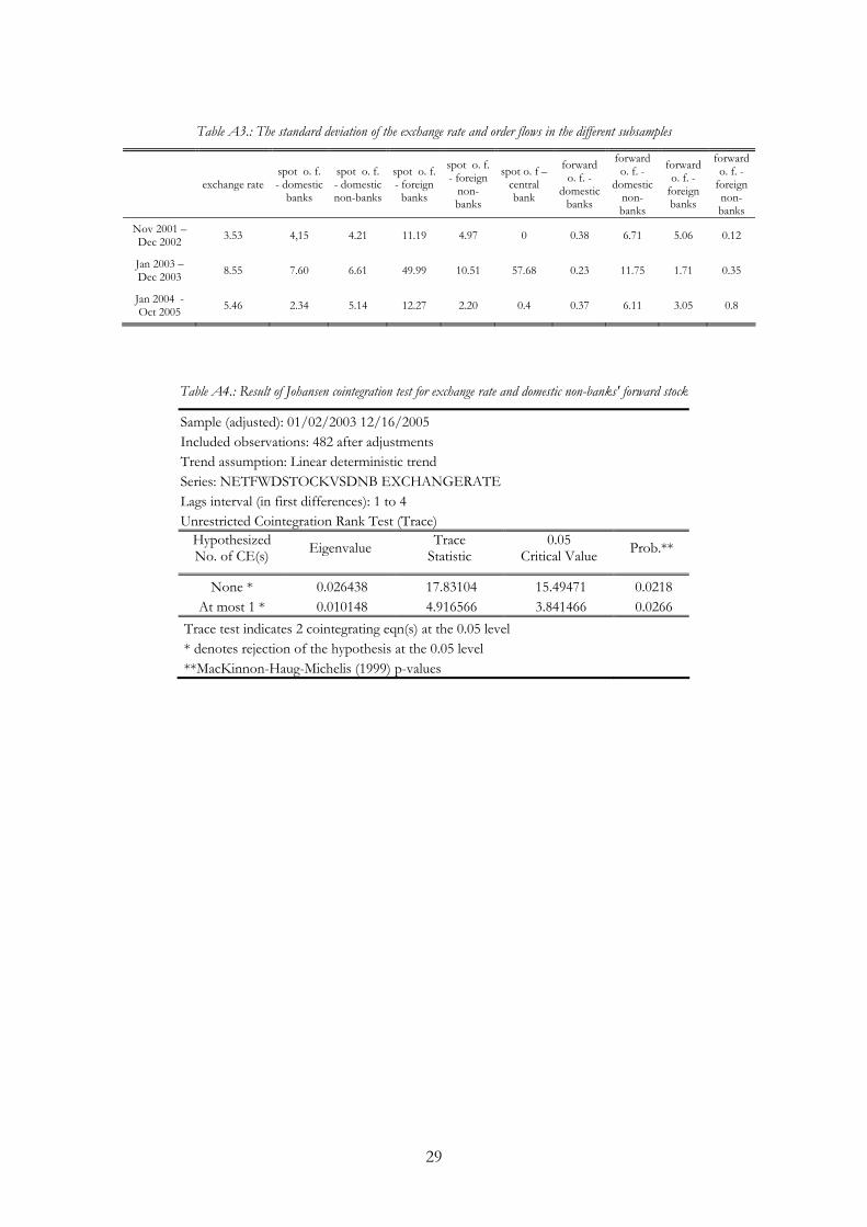
29

Table A3.: The standard deviation of the exchange rate and order flows in the different subsamples

exchange ratespot o. f. - domestic

banks

spot o. f. - domestic non-banks

spot o. f. - foreign

banks

spot o. f. - foreign

non-banks

spot o. f – central bank

forward o. f. -

domestic banks

forward o. f. -

domestic non-banks

forward o. f. -

foreign banks

forward o. f. -

foreign non-banks

Nov 2001 – Dec 2002 3.53 4,15 4.21 11.19 4.97 0 0.38 6.71 5.06 0.12

Jan 2003 – Dec 2003 8.55 7.60 6.61 49.99 10.51 57.68 0.23 11.75 1.71 0.35

Jan 2004 - Oct 2005 5.46 2.34 5.14 12.27 2.20 0.4 0.37 6.11 3.05 0.8

Table A4.: Result of Johansen cointegration test for exchange rate and domestic non-banks' forward stock

Sample (adjusted): 01/02/2003 12/16/2005 Included observations: 482 after adjustments Trend assumption: Linear deterministic trend Series: NETFWDSTOCKVSDNB EXCHANGERATE Lags interval (in first differences): 1 to 4 Unrestricted Cointegration Rank Test (Trace)

Hypothesized No. of CE(s) Eigenvalue Trace

Statistic 0.05

Critical Value Prob.**

None * 0.026438 17.83104 15.49471 0.0218 At most 1 * 0.010148 4.916566 3.841466 0.0266

Trace test indicates 2 cointegrating eqn(s) at the 0.05 level * denotes rejection of the hypothesis at the 0.05 level **MacKinnon-Haug-Michelis (1999) p-values