customer choice - personal.psu.edu · discount r1 0 0 r2 0 0 r3 0 0 r4 0 0 ... linear approximation...
TRANSCRIPT

Customer choice

Customer choice
Outline The binary choice model
□ Illustration
□ Specification of the binary choice model
□ Interpreting the results of binary choice models
□ ME output
The multinomial choice model
□ Illustration
□ Specification of the multinomial choice model
□ Interpreting the results of multinomial choice models
□ ME output
□ Properties of the multinomial choice model
Extensions of the basic choice model

Customer choice
The binary choice model: An illustration
Assume we have data on a consumer’s choice of a particular brand (1 when
the brand was chosen, 0 otherwise) across 30 purchase occasions; we also
know whether the brand was on sale on a particular occasion (0, 10, 15, 20,
or 30 cents below the regular price).
Observations / Choice data
Choice (0/1)
Discount
R1 0 0
R2 0 0R3 0 0R4 0 0R5 0 0
R6 0 0R7 0 0
R8 1 0
R9 0 10R10 0 10R11 0 10R12 0 10
R13 0 10R14 0 10
R15 1 10
Observations / Choice data
Choice (0/1)
Discount
R16 0 15
R17 0 15R18 0 15R19 1 15R20 1 15
R21 1 15R22 0 20
R23 1 20
R24 1 20R25 1 20R26 1 20R27 1 30
R28 1 30R29 1 30
R30 1 30
Customer choice
The binary choice model: An illustration
(cont’d)
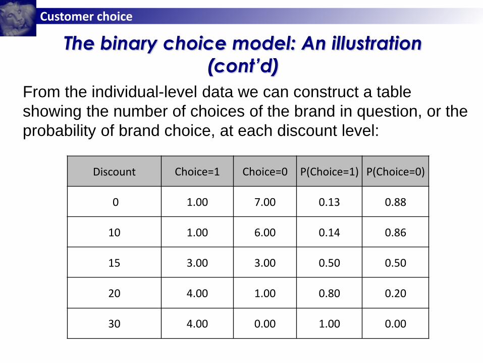
Discount Choice=1 Choice=0 P(Choice=1) P(Choice=0)
0 1.00 7.00 0.13 0.88
10 1.00 6.00 0.14 0.86
15 3.00 3.00 0.50 0.50
20 4.00 1.00 0.80 0.20
30 4.00 0.00 1.00 0.00
From the individual-level data we can construct a table
showing the number of choices of the brand in question, or the
probability of brand choice, at each discount level:

Customer choice
Probability(Choice=1) as a function of
discount size

Customer choice
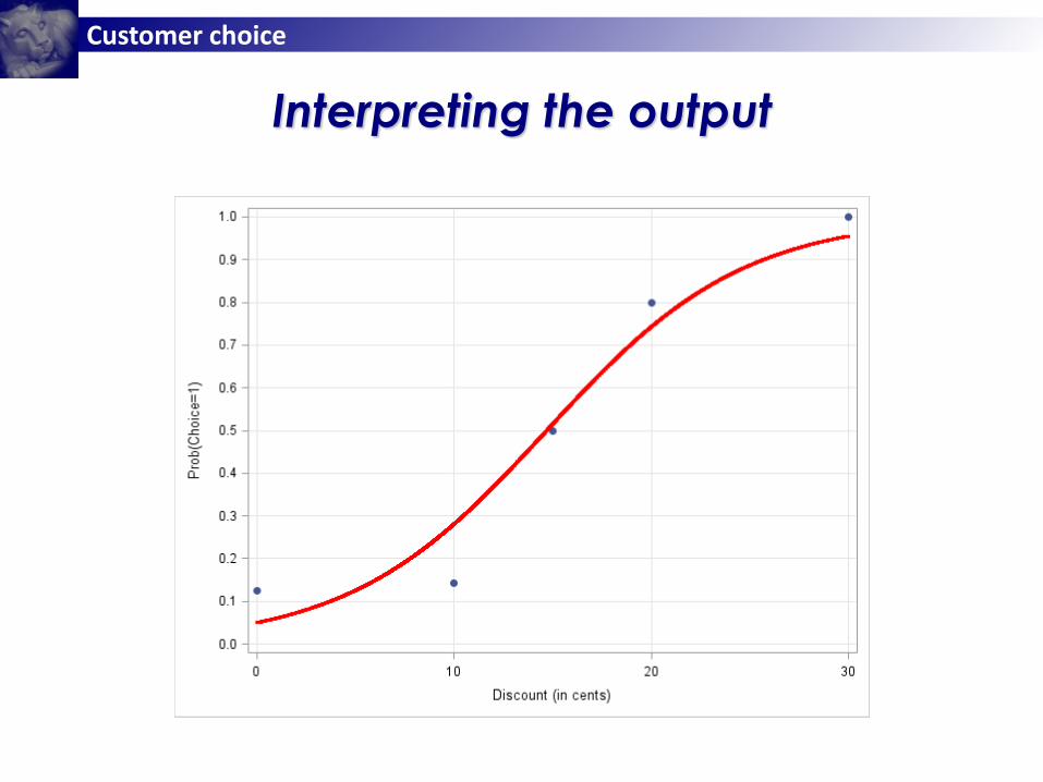
Two issues:
□ If the discount is larger than 30 cents, the model
predicts a probability greater than 1.
□ We can only compute a probability if we have multiple
0/1 observations for each level of discount.
Solution:
□ Choose an S-shaped curve that restricts the
probability of choice to the interval of 0 to 1.
□ Assume that the 0/1 variable is a crude measure of
an underlying probability of choice.
The binary choice model: An illustration
(cont’d)

Customer choice
Using an S-shaped function to link the
probability of choice to level of discount

Customer choice
In general, the logit model is:
𝑃 𝑌 = 1 =𝑒𝑥𝑝 𝛼 + 𝛽1𝑥1 + 𝛽2𝑥2 + …+ 𝛽𝑘𝑥𝑘
1 + 𝑒𝑥𝑝 𝛼 + 𝛽1𝑥1 + 𝛽2𝑥2 + …+ 𝛽𝑘𝑥𝑘
=1
1 + 𝑒𝑥𝑝 −(𝛼 + 𝛽1𝑥1 + 𝛽2𝑥2 + …+ 𝛽𝑘𝑥𝑘)
□ is an intercept term that determines P(Y=1) when all
explanatory variables xi equal zero
□ i is the contribution of a unit change in xi to P(Y=1) (for a
given value of the other explanatory variables)
The binary (logit) choice model

Customer choice
The previous model is equivalent to:
𝑙𝑜𝑔𝑖𝑡 𝑃 𝑌 = 1 = 𝑙𝑜𝑔𝑃 𝑌 = 1
1 − 𝑃 𝑌 = 1= 𝛼 + 𝛽1𝑥1 + 𝛽2𝑥2 + …+ 𝛽𝑘𝑥𝑘
■ The logit of P(Y=1) is defined as the natural logarithm of the odds
of choice and is a linear function of the explanatory variables.
■ The interpretation of the i coefficients is straightforward, but
thinking in terms of logits is not straightforward.
The binary (logit) choice model (cont’d)

Customer choice
A utility interpretation of the logit model
A consumer’s utility (u) for the brand in question consists of a
deterministic (v) and stochastic () component:
𝑢 = 𝑣 + 𝜖
The deterministic component is a linear function of observable
characteristics of the brand:
𝑣 = 𝛼 + 𝛽1𝑥1 + 𝛽2𝑥2 + …+ 𝛽𝑘𝑥𝑘
The brand is chosen if the utility of choosing the brand is
greater than the utility of not choosing the brand.
The deterministic component of the utility of not choosing the
brand is fixed at zero.
is the deterministic component of utility for the brand when
all the observable characteristics are zero.
The i are the relative contributions of the xi to the brand’s
deterministic component of utility.

Customer choice
Interpreting the results of a
binary choice model
Linear approximation interpretation of the effects of the
explanatory variables:
□ The approximate rate of change in P(Y=1) for a unit
increase in xi (holding the other x’s constant) is given by
𝛽𝑖𝑃 𝑌 = 1 1 − 𝑃(𝑌 = 1)

Customer choice
Interpreting the results of a
binary choice model
Odds ratio interpretation:
□ For given values of the other explanatory variables, a unit
increase in xi changes the odds by a factor of exp(𝛽𝑖)
Elasticity interpretation:
□ For given values of the other explanatory variables, the
percent change in the probability of choice due to a one
percent increase in xi is:
𝛽𝑖 1 − 𝑃(𝑌 = 1) 𝑥𝑖
□ Not that this implies that elasticities are greater at lower
choice probabilities.

Customer choice
Using ME to estimate a binary logit model

Customer choice
Illustrative example:
ME output (Segment tab)
Coefficient Estimates [segment 1]Coefficient estimates of the Choice model. Coefficients in bold are statistically significant.
Variables / Coefficient estimatesCoefficient estimates
Standard deviation
t-statistic
Discount 0.199905 0.075153 2.659987Const-1 -2.93693 1.138345 -2.58Baseline n/a n/a
Elasticities [segment 1]Elasticities of coefficients.
Elasticities of Discount ResponseDummy (No
Choice)
Response 0.931691 -0.71248
Dummy (No Choice) 0 0

Customer choice
How to interpret the ME output
What’s the interpretation of the intercept (-2.94)?
What’s the probability of choice at a discount of 0?
What’s the interpretation of the slope (.20)?
What is the effect of a one-cent increase in the size of
the discount on the odds of choice?
If the current discount is 12.67 cents and we increase
the discount by one cent, what is the effect on the
probability of choice?
What is the percentage change in the probability of
choice due to a 1% increase in the size of the discount?
What is the percentage change in the probability of not
choosing the brand due to a 1% increase in the size of
the discount?

Customer choice
Interpreting the output
When there is not discount, the deterministic component of the utility
for the brand is -2.94; since the deterministic component of the utility
for no choice is 0, this implies that the probability of choice is low (in
fact, it is .05).
A one cent discount increases the log of the odds of choice by .20.
A one cent discount increases the odds of choice by a factor of
exp(.20) = 1.22 (i.e., by 22%)
The probability of choice increases with the level of discount; at a
discount of 15 cents, the probability of choice is about .50.
The effect of a one cent discount on the probability of choice
depends on the price at which the brand is offered; for example, at
the mean discount of 12.67 cents, a discount of one cent will
increase the probability of choice by about .05.
The discount elasticity also depends on the price at which the brand
is offered, but the average aggregate elasticity is .93.
Customer choice
Interpreting the output

Customer choice
Variable Averages
Averages of independent variables for each alternative. Alternative-specific constants, if added, are set to zero by definition.
Variables / Alternatives Discount
Response 12.667
Dummy (No Choice) 0.000
Variable Averages for Chosen Alternatives
Averages of independent variables for each alternative where that alternative was the chosen alternative. Alternative-specific constants, if added, are set to zero by definition.
Variables / Alternatives Discount
Response 19.615
Dummy (No Choice) 7.353
Confusion Matrix on Estimation Sample
Comparison of observed choices and predicted choices (based on MNL analysis).High values in the diagonal of the confusion matrix (in bold), compared to the non-diagonal values, indicate high convergence between observations and predictions.Analysis has been performed on the estimation dataset, and measures the goodness-of-fit of the model.
Observed / Predicted Choice Response Dummy (No Choice)
Response 11 4
Dummy (No Choice) 2 13
Illustrative example: ME output (Diagnosis tab)

Customer choice
Respondents / Choice probabilitiesResponse
probabilityDummy (No
Choice) probabilityPredicted Response
Predicted Dummy (No Choice)
Observed Response
Observed Dummy (No Choice)
R1 0.050 0.950 0 1 0 1
R2 0.050 0.950 0 1 0 1
R3 0.050 0.950 0 1 0 1
R4 0.050 0.950 0 1 0 1
R5 0.050 0.950 0 1 0 1
R6 0.050 0.950 0 1 0 1
R7 0.050 0.950 0 1 0 1
R8 0.050 0.950 0 1 1 0
R9 0.281 0.719 0 1 0 1
R10 0.281 0.719 0 1 0 1
R11 0.281 0.719 0 1 0 1
R12 0.281 0.719 0 1 0 1
R13 0.281 0.719 0 1 0 1
R14 0.281 0.719 0 1 0 1
R15 0.281 0.719 0 1 1 0
R16 0.515 0.485 1 0 0 1
R17 0.515 0.485 1 0 0 1
R18 0.515 0.485 1 0 0 1
R19 0.515 0.485 1 0 1 0
R20 0.515 0.485 1 0 1 0
R21 0.515 0.485 1 0 1 0
R22 0.743 0.257 1 0 0 1
R23 0.743 0.257 1 0 1 0
R24 0.743 0.257 1 0 1 0
R25 0.743 0.257 1 0 1 0
R26 0.743 0.257 1 0 1 0
R27 0.955 0.045 1 0 1 0
R28 0.955 0.045 1 0 1 0
R29 0.955 0.045 1 0 1 0
R30 0.955 0.045 1 0 1 0
Illustrative example: ME output (Estimation tab)

Customer choice
Interpreting the output
The fit of the logit model can be assessed based on
the confusion matrix, which cross-classifies
observed and predicted choices.
If the predicted probability of choice exceeds .5,
then 𝑌 = 1, otherwise 𝑌 = 0.
The sum of the diagonals over the sample size gives
the hit rate (percent of observations for which the
actual choice was predicted correctly).
In the illustration, the hit rate is 80%.

Customer choice
Review: Basic idea of the
binary choice model
What determines choice when there are two choice
options?
Assume we have two possible influences on the choice
of a brand, quality and price. The model is
𝑃 𝑌 = 1 =1
1 + 𝑒𝑥𝑝 −(𝛼 + 𝛽1𝑄 + 𝛽2𝑃)
We can rewrite this equation as follows:
𝑙𝑜𝑔𝑃 𝑌 = 1
1 − 𝑃 𝑌 = 1= 𝛼 + 𝛽1𝑄 + 𝛽2𝑃

Customer choice
Evaluating the effect of quality on choice
Model Effect of a unit change in Q
𝑃 𝑌 = 1 =1
1 + 𝑒𝑥𝑝 −(𝛼 + 𝛽1𝑄 + 𝛽2𝑃)
Linear approximation:
𝛽1 𝑌 = 1 1 − 𝑃(𝑌 = 1)
Elasticity:
𝛽1 1 − 𝑃(𝑌 = 1) 𝑄
𝑃 𝑌 = 1
1 − 𝑃 𝑌 = 1= exp(𝛼 + 𝛽1𝑄 + 𝛽2𝑃) exp(𝛽1)
𝑙𝑜𝑔𝑖𝑡 𝑃 𝑌 = 1 = 𝑙𝑜𝑔𝑃 𝑌 = 1
1 − 𝑃 𝑌 = 1
= 𝛼 + 𝛽1𝑄 + 𝛽2𝑃
𝛽1

Customer choice
The multinomial choice model: An illustration
Observations / Choice data
AlternativesChoice (0/1)
Discount
1 A 0 0
B 0 0
C 1 0
2 A 1 5
B 0 0
C 0 0
3 A 0 5
B 0 0
C 1 0
4 A 1 30
B 0 0
C 0 0
5 A 0 15
B 0 0
C 1 0
6 A 0 0
B 0 0
C 1 0
7 A 0 0
B 0 0
C 1 0
8 A 1 15
B 0 0
C 0 0
9 A 1 15
B 0 0
C 0 0
10 A 1 25
B 0 0
C 0 0
Observations / Choice data
AlternativesChoice (0/1)
Discount
11 A 0 0
B 0 10
C 1 0
12 A 0 0
B 0 10
C 1 0
13 A 0 0
B 0 10
C 1 0
14 A 0 0
B 1 15
C 0 0
15 A 0 0
B 0 15
C 1 0
16 A 0 0
B 0 15
C 1 0
17 A 0 0
B 1 20
C 0 0
18 A 0 0
B 1 30
C 0 0
19 A 0 0
B 1 20
C 0 0
20 A 0 0
B 1 30
C 0 0
Observations / Choice data
AlternativesChoice (0/1)
Discount
21 A 1 30
B 0 5
C 0 0
22 A 1 20
B 0 5
C 0 0
23 A 1 25
B 0 15
C 0 0
24 A 1 20
B 0 5
C 0 0
25 A 0 15
B 1 10
C 0 0
26 A 0 5
B 1 25
C 0 0
27 A 1 10
B 0 30
C 0 0
28 A 0 15
B 1 30
C 0 0
29 A 0 5
B 0 25
C 1 0
30 A 0 10
B 1 30
C 0 0
Assume we have data on a consumer’s choice of one of three brands across 30
purchase occasions and we also know whether the brands were on sale on a
particular occasion (0 to 30 cents below the regular price).

Customer choice
In general, the multinomial model is:
𝑃 𝑌 = 𝑖 =𝑒𝑥𝑝 𝛼𝑖 + 𝛽1𝑥𝑖1 + 𝛽2𝑥𝑖2 + …+ 𝛽𝑘𝑥𝑖𝑘
𝑖 𝑒𝑥𝑝 𝛼𝑖 + 𝛽1𝑥𝑖1 + 𝛽2𝑥𝑖2 + …+ 𝛽𝑘𝑥𝑖𝑘
The probability of choice of alternative i is equal to the
share of alternative i’s exponentiated deterministic utility
component among all choice alternatives.
For identification, exp(·) is set to one for one brand.
The interpretation of the coefficients is the same as in
the binary logit model
The multinomial choice model

Customer choice
Using ME to estimate a multinomial logit model

Customer choice
Illustrative example: ME output (Diagnosis tab)
Variable AveragesAverages of independent variables for each alternative. Alternative-specific constants, if added, are set to zero by definition.
Variables / Alternatives Discount
A 8.833
B 11.833C 0.000
Variable Averages for Chosen AlternativesAverages of independent variables for each alternative where that alternative was the chosen alternative. Alternative-specific constants, if added, are set to zero by definition.
Variables / Alternatives Discount
A 19.500B 23.333C 0.000
Confusion Matrix on Estimation SampleComparison of observed choices and predicted choices (based on MNL analysis).
High values in the diagonal of the confusion matrix (in bold), compared to the non-diagonal values, indicate high convergence between observations and predictions.
Analysis has been performed on the estimation dataset, and measures the goodness-of-fit of the model.
Observed / Predicted Choice A B C
A 8 1 1B 1 7 1C 1 1 9

Customer choice
Illustrative example: ME output (Estimation tab)Respondents / Choice
probabilitiesA probability B probability C probability Predicted A Predicted B Predicted C Observed A Observed B Observed C
1 0.099 0.025 0.875 0 0 1 0 0 1
2 0.234 0.022 0.744 0 0 1 1 0 0
3 0.234 0.022 0.744 0 0 1 0 0 1
4 0.980 0.001 0.019 1 0 0 1 0 0
5 0.702 0.008 0.290 1 0 0 0 0 1
6 0.099 0.025 0.875 0 0 1 0 0 1
7 0.099 0.025 0.875 0 0 1 0 0 1
8 0.702 0.008 0.290 1 0 0 1 0 0
9 0.702 0.008 0.290 1 0 0 1 0 0
10 0.948 0.001 0.051 1 0 0 1 0 0
11 0.085 0.167 0.748 0 0 1 0 0 1
12 0.085 0.167 0.748 0 0 1 0 0 1
13 0.085 0.167 0.748 0 0 1 0 0 1
14 0.066 0.357 0.577 0 0 1 0 1 0
15 0.066 0.357 0.577 0 0 1 0 0 1
16 0.066 0.357 0.577 0 0 1 0 0 1
17 0.040 0.606 0.354 0 1 0 0 1 0
18 0.008 0.922 0.070 0 1 0 0 1 0
19 0.040 0.606 0.354 0 1 0 0 1 0
20 0.008 0.922 0.070 0 1 0 0 1 0
21 0.979 0.002 0.019 1 0 0 1 0 0
22 0.861 0.010 0.128 1 0 0 1 0 0
23 0.920 0.031 0.049 1 0 0 1 0 0
24 0.861 0.010 0.128 1 0 0 1 0 0
25 0.664 0.061 0.275 1 0 0 0 1 0
26 0.052 0.783 0.165 0 1 0 0 1 0
27 0.058 0.875 0.067 0 1 0 1 0 0
28 0.146 0.794 0.060 0 1 0 0 1 0
29 0.052 0.783 0.165 0 1 0 0 0 1
30 0.058 0.875 0.067 0 1 0 0 1 0

Customer choice
Illustrative example:
ME output (Segment tab)Coefficient Estimates [segment 1]Coefficient estimates of the Choice model. Coefficients in bold are statistically significant.
Variables / Coefficient estimates Coefficient estimates Standard deviation t-statistic
Discount 0.203877 0.052848 3.857763Const-1 -2.17458 0.797709 -2.72604Const-2 -3.53879 1.158237 -3.05533Baseline n/a n/a
Elasticities [segment 1]Elasticities of coefficients.
Elasticities of Discount A B C
A 0.547463 -0.11885 -0.40045B -0.24913 1.110283 -0.68194
C 0 0 0

Customer choice
Properties of the MNL model:
Independence of irrelevant alternatives (IIA)
This assumption implies that when a new alternative
is added to a choice set, the new alternative will
steal share from the existing alternatives in
proportion to their current choice shares.
This is unrealistic because a new alternative is likely
to steal more share from more similar alternatives
(e.g., if a new cola drink is introduced, existing cola
drinks are likely more vulnerable than non-cola
drinks).
To avoid this problem, the choice alternatives can
be grouped into sets that are similar.

Customer choice
Office Star Choice Data
Data are available for 20 respondents who made a
choice between 3 alternatives: Office Star, Paper &
Co., and Office Equipment;
Five variables are used to predict people’s choices:
the number of purchases previously made at one of
the stores, ratings of whether a given store is
expensive or convenient, and whether a store offers
good service and a large choice;

Customer choice
Office Star choice data (cont’d)Observations / Choice
dataAlternatives
Choice
(0/1)
Past
purchasesExpensive Convenient Service Large choice
Respondent 1 OfficeStar 0 0 2 1 3 4
Paper & Co 0 0 4 4 7 3
Office Equip'nt 1 0 1 3 5 1
Respondent 2 OfficeStar 1 0 3 2 5 6
Paper & Co 0 0 7 4 6 7
Office Equip'nt 0 0 5 5 5 7
Respondent 3 OfficeStar 1 0 3 3 3 6
Paper & Co 0 0 7 2 1 1
Office Equip'nt 0 0 5 2 1 7
Respondent 4 OfficeStar 0 0 1 7 7 4
Paper & Co 1 8 3 4 7 7
Office Equip'nt 0 0 6 5 2 1
Respondent 5 OfficeStar 0 0 5 2 2 4
Paper & Co 1 0 1 3 3 4
Office Equip'nt 0 0 7 1 2 7
Respondent 6 OfficeStar 1 0 7 6 4 3
Paper & Co 0 0 5 5 2 3
Office Equip'nt 0 0 5 2 6 2
Respondent 7 OfficeStar 0 0 5 2 7 4
Paper & Co 1 0 4 4 3 4
Office Equip'nt 0 0 1 7 5 2
Respondent 8 OfficeStar 1 0 1 7 3 6
Paper & Co 0 0 3 6 2 4
Office Equip'nt 0 0 5 1 1 7
Respondent 9 OfficeStar 1 0 4 4 4 4
Paper & Co 0 0 4 3 3 6
Office Equip'nt 0 0 1 4 4 1
Respondent 10 OfficeStar 1 0 3 2 3 2
Paper & Co 0 0 7 3 1 4
Office Equip'nt 0 0 1 5 5 1
Etc.

Customer choice
Office Star data: Diagnosis tabVariable AveragesAverages of independent variables for each alternative. Alternative-specific constants, if added, are set to zero by definition.
Variables / Alternatives Past purchases Expensive Convenient Service Large choice
OfficeStar 0.000 3.150 3.950 3.300 4.550Paper & Co 0.900 3.750 3.600 4.250 4.350Office Equip'nt 0.800 3.900 4.400 3.500 4.050
Variable Averages for Chosen AlternativesAverages of independent variables for each alternative where that alternative was the chosen alternative. Alternative-specific constants, if added, are set to zero by definition.
Variables / Alternatives Past purchases Expensive Convenient Service Large choice
OfficeStar 0.000 2.700 4.400 3.400 4.900Paper & Co 2.250 2.875 3.625 4.625 5.000Office Equip'nt 4.000 3.000 4.000 4.000 3.500
Confusion Matrix on Estimation SampleComparison of observed choices and predicted choices (based on MNL analysis).High values in the diagonal of the confusion matrix (in bold), compared to the non-diagonal values, indicate high convergence between observations and predictions. Analysis has been performed on the estimation dataset, and measures the goodness-of-fit of the model.
Observed / Predicted Choice OfficeStar Paper & Co Office Equip'nt
OfficeStar 10 1 1Paper & Co 0 7 0Office Equip'nt 0 0 1

Customer choice
Office Star Data: Estimation tabEstimation Sample DetailsChoice probabilities, predicted and observed choices, segment membership probabilities and predicted segment for the sample usedto estimate the model.
Respondents / Choice probabilities
OfficeStar probability
Paper & Co probability
Office Equip'nt
probability
Predicted OfficeStar
Predicted Paper & Co
Predicted Office
Equip'nt
Observed OfficeStar
Observed Paper & Co
Observed Office
Equip'nt
Respondent 1 0.628 0.353 0.020 1 0 0 0 0 1
Respondent 2 0.900 0.083 0.017 1 0 0 1 0 0
Respondent 3 0.998 0.001 0.002 1 0 0 1 0 0
Respondent 4 0.015 0.985 0.000 0 1 0 0 1 0
Respondent 5 0.040 0.960 0.000 0 1 0 0 1 0
Respondent 6 0.506 0.491 0.003 1 0 0 1 0 0
Respondent 7 0.251 0.388 0.361 0 1 0 0 1 0
Respondent 8 0.982 0.018 0.000 1 0 0 1 0 0
Respondent 9 0.637 0.338 0.025 1 0 0 1 0 0
Respondent 10 0.748 0.038 0.215 1 0 0 1 0 0
Respondent 11 0.039 0.960 0.001 0 1 0 0 1 0
Respondent 12 0.009 0.164 0.827 0 0 1 0 0 1
Respondent 13 0.779 0.221 0.000 1 0 0 1 0 0
Respondent 14 0.955 0.042 0.003 1 0 0 1 0 0
Respondent 15 0.719 0.000 0.281 1 0 0 1 0 0
Respondent 16 0.669 0.322 0.009 1 0 0 0 1 0
Respondent 17 0.088 0.904 0.008 0 1 0 0 1 0
Respondent 18 0.879 0.117 0.004 1 0 0 1 0 0
Respondent 19 0.051 0.725 0.224 0 1 0 0 1 0
Respondent 20 0.109 0.891 0.000 0 1 0 0 1 0

Customer choice
Office Star Data: Segment tab
Coefficient Estimates [segment 1]
Coefficient estimates of the Choice model. Coefficients in bold are statistically significant.
Variables / Coefficient estimatesCoefficient estimates
Standard deviation
t-statistic
Past purchases 0.863569 0.359493 2.402184
Expensive -0.81508 0.383513 -2.12529
Convenient 0.537433 0.373534 1.438779
Service 0.166118 0.255744 0.649551
Large choice 0.4312 0.32222 1.338216
Const-1 4.391705 1.933972 2.270821
Const-2 3.600351 1.805345 1.994273
Baseline n/a n/a

Customer choice
Office Star Data: Segment tab (cont’d)
Elasticities [segment 1]Elasticities of coefficients.
Elasticities of Past purchases OfficeStar Paper & Co Office Equip'nt
OfficeStar 0 0 0Paper & Co -0.06699 0.084338 -0.00238Office Equip'nt -0.14645 -0.1145 1.190273
Elasticities of Expensive OfficeStar Paper & Co Office Equip'nt
OfficeStar -0.65391 0.672727 0.578669Paper & Co 0.553199 -0.82619 0.538747Office Equip'nt 0.054357 0.111399 -0.71738
Elasticities of Convenient OfficeStar Paper & Co Office Equip'nt
OfficeStar 0.494317 -0.47137 -0.5861Paper & Co -0.34876 0.581375 -0.58167Office Equip'nt -0.16315 -0.20024 1.616706

Customer choice
Office Star Data: Segment tab (cont’d)
Elasticities [segment 1]Elasticities of coefficients.
Elasticities of Service OfficeStar Paper & Co Office Equip'nt
OfficeStar 0.135179 -0.11152 -0.22981Paper & Co -0.12049 0.194688 -0.17631Office Equip'nt -0.04354 -0.05058 0.420012
Elasticities of Large choice OfficeStar Paper & Co Office Equip'nt
OfficeStar 0.416223 -0.38783 -0.52979Paper & Co -0.34915 0.558712 -0.48908Office Equip'nt -0.03802 -0.12612 0.694574

Customer choice
Extensions of the basic choice model
The logit model assumes that the intercepts and the
effects of the explanatory variables in the
deterministic part of utility are the same across
individuals.
Two ways to get around this limitation:
□ Individual differences can be used as additional
determinants of the deterministic part of utility.
□ Different coefficients can be estimated for different
segments of consumers (so-called latent class choice
models).