Stock Trading using Linear Genetic Programmingwith Multiple Time Frames

Garnett WilsonAfinin Labs Inc.

St. John’s, Canadagwilson@afinin.com

Derek LeblancAfinin Labs Inc.

St. John’s, Canadadleblanc@afinin.com

Wolfgang BanzhafAfinin Labs Inc.

St. John’s, Canadabanzhaf@afinin.com

ABSTRACTA number of researchers have attempted to take successfulGP trading systems and make them even better throughthe use of filters. We investigate the use of a linear geneticprogramming (LGP) system that combines GP signals pro-vided over multiple intraday time frames to produce onetrading action. Four combinations of time frames stretchingfurther into the past are examined. Two different decisionmechanisms for evaluating the overall signal given the GPsignals over all time frames are also examined, one basedon majority vote and another based on temporal proxim-ity to the buying decision. Results indicated that majorityvote outperformed emphasis on proximity of time frames tothe current trading decision. Analyses also indicated thatlonger time frame combinations were more conservative andoutperformed shorter combinations for both overall upwardand downward price trends.

Categories and Subject DescriptorsI.2.8 [Artificial Intelligence]: Problem Solving, ControlMethods, and Search—Heuristic methods

General TermsAlgorithms, Performance, Experimentation

Keywordscomputational finance, linear genetic programming, algo-rithmic trading

1. INTRODUCTIONResearchers who apply genetic programming (GP) or evo-

lutionary computation methods for analysis of financial mar-kets have a number of different approaches to discover prof-itable opportunities in the price time series they analyze.Some researchers train a system on an extended period oftime, and then allow the evolved solution of static rules to

Permission to make digital or hard copies of all or part of this work forpersonal or classroom use is granted without fee provided that copies arenot made or distributed for profit or commercial advantage and that copiesbear this notice and the full citation on the first page. To copy otherwise, torepublish, to post on servers or to redistribute to lists, requires prior specificpermission and/or a fee.GECCO’11, July 12–16, 2011, Dublin, Ireland.Copyright 2011 ACM 978-1-4503-0557-0/11/07 ...$10.00.

operate on a subsequent extended test period [3], [4]. Otherresearchers have found it beneficial to continually train ona moving window, and only act in anticipation of the im-mediate future of the price changes based on the immediatepast [1], [8]. Others go further than this, combining eitherof these systems with filters that are used to improve theconfidence that a GP signal is actually being evolved on aninherently trending time series [3], [4], [7]. In this work,we combine the notions of filtering GP signals and movingwindows of varying length in a linear genetic programmingsystem (LGP). In particular, we use the LGP system to de-termine whether price series in partially overlapping timeframes are collectively consistent in producing a particularalgorithm signal.

The next section describes existing literature on the useof filters with GP and the notion of predictable windowswith price series. Section 3 describes the linear GP systemapplied to stock trading using multiple time frames. Section4 describes trading performance characteristics of the systemand its profitability. Conclusions follow in Section 6.

2. PREVIOUS WORKTo the authors’ knowledge there are no GP systems in the

literature that run over multiple time frames to create moreaccurate signals. However, there are a few examples of theapplication of pretests to market data used in conjunctionwith evolutionary computing to determine if the price se-ries is predictable (and thus appropriate for GP analysis).The first instance of a GP system with filtering applied toa financial domain was Kaboudan [4]. Kaboudan proposeda metric called the “η” statistic that indicates predictabil-ity. To establish η, a GP used the unaltered price series anda shuffled version of the price series. The sum of squarederrors (SSE) between the results predicted by GP and theunaltered price series is calculated, and compared to the SSEof the GP and the randomly shuffled series over numerousGP trials. Kaboudan examined the price series of eight DowJones stocks and found that predictability was inversely re-lated to time elapsed between price samplings. Chen et al.[3] expand on Kaboudan’s work by comparing GP results todifferent search methods rather than running GP on shuf-fled time series. The authors compare GP to both intensiverandom search and a search method called “lottery” tradingbased on a random variable. The comparison of GP to theserandom search methods accurately indicated predictabilityof the time series in some of the nine markets tested. Neelyand Weller [6] used GP to attempt to forecast the volatilityof future currency prices in a time series rather than future

1667

prices themselves, but they found that the technique was notmore useful than recognized technical volatility measures.

Rather than testing predictability of time series using GP,other researchers have attempted to restrict GP signals toimprove their accuracy. Li and Tsang [5] use a GP hybridcalled “FGP” that includes decision trees of rule sets. TheGP was given a minimum and maximum of signals that werepermitted when predicting prices based on the training data.The authors reported that the failure rate was reduced, butthey also found that there were more missed opportunitiesby the system.

In this work we do not train GP on shuffled versions ofactual price series or compare results of GP to randomizedsearch techniques to increase confidence in underlying pre-dictability of a price series. In contrast, we use GP multipletimes, each time on a separate unaltered time series. Thetime series are progressively longer in order to increase theconfidence that the GP is making a signal based on a moresustained trend.

3. LGP MULTIPLE TIME FRAMETRADING SYSTEM

3.1 LGP Algorithm and ParametersThe algorithm applied to stock trading in this work is lin-

ear genetic programming (LGP). LGP evolves individualscomposed of binary strings and associated registers, in con-trast to the tree-based individuals of traditional GP. Thebits that make up one individual can be further divided intoseparate instructions. These instructions can be executedsequentially, with the subresult of each instruction stored inone of the individual’s registers. Each instruction performsan operation corresponding to a member of the function setthat it references, and uses subresults in registers or externaldata as operands. Thus, each LGP individual represents asmall machine-language type program that is evaluated bya fitness function upon termination, often by examining a fi-nal solution in one of the individual’s registers. LGP is nowconsidered an established hallmark form of GP, and furtherdetails of general LGP implementation can be found in [2].

In this work, we apply a LGP automated trading imple-mentation to the intraday trading of four stocks: BRK-B,RIMM, RY, and AAPL. An initial period was reserved toestablish values of technical indicators, following which theGP fitness was evaluated on data corresponding to a mov-ing window of n minutes. Individuals represented sets oftrading rules, based on functions in the function set (to bedescribed). For each window of trading minutes m to n,each of m to n - 1 minutes were used for calculation of atrading decision, with m + 1 to n left for the evaluation ofthe signal based on the preceding minutes. Data used for thedetermination of a trading decision were normalized usingtwo-phase preprocessing similar to treatment of stock datain [1]: All daily values were transformed by division usinga lagged moving average, and then normalized using linearscaling into the range [0, 1] using

vscaled =vt − lnhn − ln

(1)

where vscaled is the normalized trading value, vt is the trans-formed trading value at time step t, hn is highest trans-formed value in the last n time steps, ln is the lowest trans-

formed value in the last n time steps, and n is the length ofthe time lag chosen for the initial transformation.

In addition to an instruction set, each LGP individualpossesses four registers, a flag for storing the current value oflogical operators, and an output (trade) register for storingthe value corresponding to a trade signal following executionof the instruction set. If the value of the trade register is0, no trade is conducted. If the value in the trade registercorresponds to a value in the range +/-[0, 1], it indicates thestrength of a buy or sell signal based on positive or negativevalue, respectively. The fitness function is the profitabilityof the GP individual after evolution over a series of priceswhen acting on a next unknown price (described in detailbelow). For each trade conducted, there is a moderate $10trading commission fee (with a round trip commission of$20).

The LGP function set includes standard mathematical op-erators and logical operators. In addition, established tech-nical analysis metrics such as moving average, momentum,and channel breakout are used. Moving average is the meanof the previous n share prices. The momentum is the ratioof a time-lagged price to the current price. Channel break-out typically uses Bollinger bands around a n-minute mov-ing average of the price at +/- 2 standard deviations of theprice movement over the last n minutes to alert the traderof significant movements in rates. Each LGP tournamentconsisted of 1000 rounds. XOR mutation on individual in-structions was used with a probability of 0.5, and crossoveroccurred with a probability of 0.9.

3.2 Multiple Time FramesThe best individual, consisting of the best trading rule

set, is used by a “live” trading algorithm. The live tradingsystem provides known information to the LGP for minutesm to n. The LGP algorithm returns a signal for the livetrading system, which is used as the basis of its trade on thefollowing minute, n + 1. The net value of the best evolvedindividual (trading rules) given the signal of the trade reg-ister over all the fitness cases is the buy or sell signal to the“live” trading system. The best LGP individual can thusrecommend a buy, sell, or hold to the live system. Based onthe signal, the live system purchases as much stock as pos-sible using its current cash assets, sells all shares, or doesnothing, respectively. The sell signal of the GP system isgenerally issued as a sell to stop losses in a downtrend, soan additional sell mechanism to take profit based on mo-mentum is used that closes the trade when a future higherprice is met following a buy signal. The transactions of thelive trading system are actually based on unknown data anddetermine the success of the automatic trader.

For a time frame of m to n minutes, there are n-1 fitnesscases. In the smallest time frame, that of 5 minutes, thereare 4 fitness cases for m = 1 to n = 5 in the 5 minutewindow and a signal is made for the unknown (6th) minutefollowing the time frame. For example, in the smallest (5minute) time frame, the LGP will train on minute 1 withminute 2 unknown, then minute 1, 2 with 3 unknown, then1, 2, 3 with 4 unknown, and finally 1, 2, 3, 4 with 5 unknown(giving 4 fitness cases in total). Based on the mean valueover all the trade registers of the best individuals after eachfitness case, the overall signal is determined. The automatedsystem then trades in anticipation of the next minute (theunknown).

1668

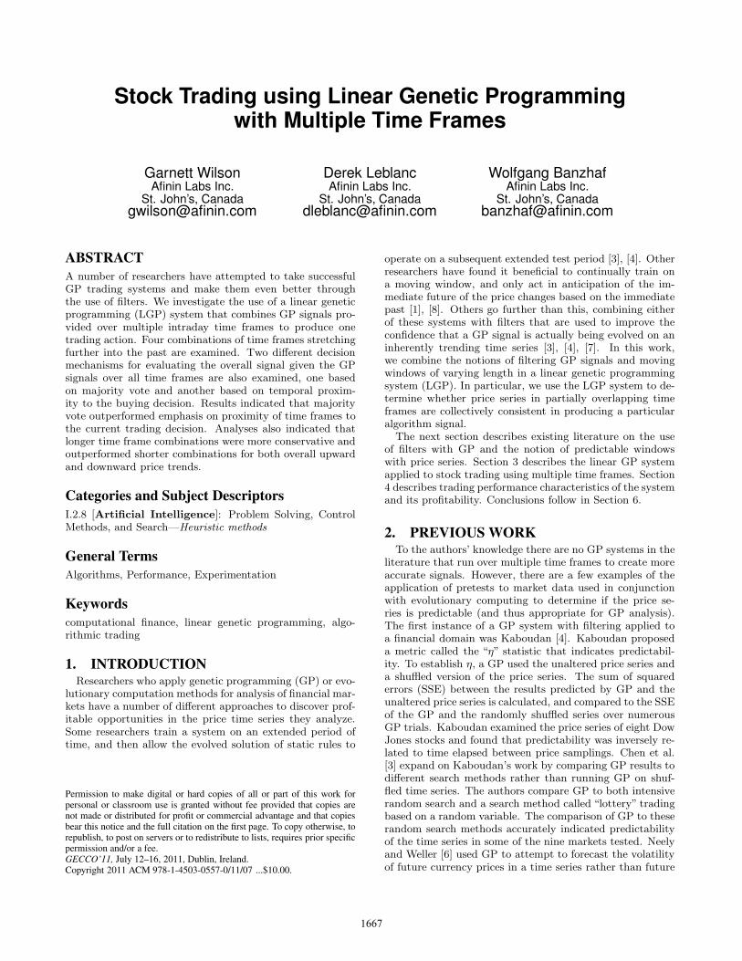
Unkown5 min10 min15 min30 min

time frame 1time frame 2time frame 3time frame 4

Figure 1: The LGP trains repeatedly on progres-sively longer time scales to generate the signal forthe “live” trading system to act on unknown values.

This smallest time frame, given minute-to-minute tradingdecisions, provides an algorithm that is reactive to change.In this paper we examine tempering the reactiveness of thesmaller time scale with additional information from GP runon longer time frames into the past. For each time frame,the LGP algorithm evaluates known (provided) values ofm to n, with minute n + 1 being unknown and GP beingrun on n - 1 fitness cases. Now there are multiple signals,which may or may not be the same, since the LGP trainsover longer time frames consisting of more fitness cases asn increases. As the number of time frames increases, therecommended action corresponds to trading strategies forlonger trends. Combining the signals for shorter and longertime frames creates a more conservative (safer) signal forbuying and selling actions. In this work, we found it usefulto examine the time frames of 5, 10, 15, and 30 minutes.The process is shown in Figure 1.

Once the GP algorithm has been run on each of the pro-gressively increasing time frames, an overall trading signalmust be determined from the signals generated by the GPfor each time frame. Two methods for deciding this actionare examined. The first decision method is called “Major-ity” and uses a buy or sell signal if that signal accounts forhalf (or more) of all the signals for each time scale. Thesecond method is called “Temporal Proximity” and uses abuy or sell signal if that signal is present for (at least) allof the time frames back from the most recent time framef to time frame f - �f/2� for f time frames. Hold signalsare not counted toward an action decision, but in the caseof both majority and temporal decision methods holds areissued if no decision can be made. The majority signal de-cision is designed to base a decision to buy or sell on anoverall trend over all the time frames, irrespective of thelatest price movement in the most current time frame. Forinstance, if the price trend has been increasing for the past30 minutes overall given four time frames and a 30 minuteand 15 minute time frame recommend buys but the verylatest time frame recommends a sell, the majority decisionrecommends a buy. There is a slight aggressiveness of thesystem toward buying: If there is a tie between buy and sell,buy takes preference. In contrast, the temporal proximitydecision emphasizes the trend closest to the unknown pricepoint. For example, temporal proximity will recommend asell if the time frame at 10 minutes and 5 minutes bothrecommend a sell given four time frames.

4. STOCK TRADING RESULTSThe live trading system is evaluated using minute interval

price values for each of 373 minutes of the arbitrarily chosentrading day, October 18, 2010. Results are shown for oneday since we are most interested in examining behavior in

high volatility, intraday situations within the space of thispaper. We use data for stocks selected for their variationsin trend, and thus stocks are examined on an individual ba-sis. Two minutes and an initial 15 minutes of values arewithheld for data feed verification and seeding of techni-cal indicators, respectively. The stock prices examined wereBRK-B (Berkshire Hathaway Class B), RIMM (Research inMotion Limited), RY (Royal Bank of Canada) , and AAPL(Apple Inc.). The stocks were chosen in order to providea number of different trends to evaluate the robustness ofthe algorithm and for the difficulty these trends present forGP: all are volatile and only one presents an upward pricemovement throughout the day that is not abrupt. Varia-tion across trials is practically non-existent since the LGPis consistent enough that it will recommend the same action(one of buy, sell, or hold) given the same price values in atime frame window, so a single run is shown. Performanceof the LGP over time is examined, followed by examinationof trading behavior and overall profitability.

4.1 Performance TrendsThe ability of the algorithm to trade over time is exam-

ined in this section. The general success of the LGP tradingsystem used in this work was previously established in [8],and in this work we are interested in focusing on the effectof multiple time frames on trading. The system starts thetrading day with $1,000,000 in cash assets. The total worth(total value of cash and shares) in dollars of the live tradingsystem using all time frames as described in the previoussection are provided in Figure 2 for each minute. As a base-line, the value of total assets when as much of the initialcash as possible is invested in shares at the start of tradingis indicated as Buy and Hold. For fairness, trading can startfor all time frame combinations only after the number ofminutes required for the longest time frame have elapsed.

The most striking aspect of Figure 2 is that when the Ma-jority and Temporal Proximity decision methods are com-pared for each stock, the majority decision process yieldsbetter results in general across time frame combinations.The less restrictive decision process of Majority allowed moretime frames to rise above the profitability of the buy-and-hold plot (solid line) compared to Temporal Proximity. Tomake the comparison with buy-and-hold clearer, the ratioof each time frame combination’s current total worth tobuy-and-hold is plotted in Figure 3 for each minute. Thesegraphs indicate that in the case of almost every stock, theratios achieved by temporal proximity decision do not reachthe levels of majority decision made by one or more of thetime frames. Based on the overall better performance of themajority decision, we now focus on its analysis.

By examining the buy-and-hold behavior of each stock’sprices, we can note from Figure 2 the behavior of each stock’sprice trend throughout the day. We see that BRK-B ex-hibits an overall sideways trend for the day, with consid-erable phases of volatility during certain periods. For thistype of price trend, we see that the {5, 10, 15} minute timeframe combination performs best. RIMM exhibits a priceseries that (overall) climbs throughout the day, but includesperiods of decline, abrupt and gradual gains, and sidewaysmovement. For this type of trend we see that the most con-servative time frame combination works best, namely {5,10, 15, 30}. RY exhibits a fairly consistent gain in pricethroughout the day, and we again find that {5, 10, 15, 30}

1669

Figure 2: Total value of assets (cash and shares held) given initial $1,000,000.

1670

Figure 3: Ratio of total assets to buy and hold given initial $1,000,000.

1671

(and {5, 10}) perform best. AAPL has a largely decliningprice trend, followed by gains in the later part of the day(prior to minute 300 until close). In order to avoid losses,the {5, 10, 15, 30} time frame combination dominates formost of the day but it is not able to realize gains at the endof the day because it was out of market during a large priceincrease that the more reactive, shorter time frame combina-tions ({5} and {5, 10}) could quickly identify. One cannotsee the buy-and-hold trend as a reference point, but Fig-ure 3 shows clearly the ranking of time frame combinationsagainst buy-and-hold throughout the day for each stock. Allresults just discussed are clearly presented, and it is evidentthat GP using multiple time frames outperforms buy-and-hold where in many instances GP using only the 5 minutetime frame may not. However, the less reactive nature ofthe longer time frame combinations does not allow them toreact to fast moving price changes toward profit and then 5outperforms others (see end of price series for RY and AAPLin Figure 3). Examining all stocks using Majority decision,the longer {5, 10, 15, 20} time frame combination domi-nates the shorter time frame combinations other than forthe case of RIMM. Overall profitability of the different timeframe combinations is discussed in greater detail in Section4.3. The reactiveness of trading behavior related to numberof time frames in a combination, which we now examine ingreater detail, directly impacts profitability.

4.2 Trading AnalysisThe profitability of the different fitness metrics are a result

of underlying length and frequency of trades conducted. Fig-ure 4 shows a chart of the trading activity for each GP andtime frame combination; both majority and time proximitydecision types are shown to determine the effect of decisiontype on trading activity. Time is graphed on the abscissa,with a trade that ends in profit (after commissions) graphedabove the abscissa and a trade that ends in a loss (after com-missions) graphed below the abscissa. These graphs allowthe reader to examine in a simple way both the total num-ber of trades made by each time scale combination, and howmany of those trades were successful. All trades shown inFigure 4 are the result of the GP algorithm issuing a signalto buy, whether or not it resulted in profit at the sell signalof the trade. The sell signal, as discussed in Section 3.2, isthe result of a sell signal to take profit or a sell signal to stopfurther losses.

It is evident from Figure 4 that for each stock, as the num-ber of time frames in a combination increases, the number oftrades decreases. Additionally, the overall time spent in themarket for each trade increases as the number of time framesin a combination increases. The temporal proximity decision(right side) did not generate any noteworthy behavior dif-ferences from the majority decision trading patterns (leftside) with respect to trade length or overall trading accu-racy. The temporal proximity decision, however, did resultin fewer trades overall, which is to be expected due to itsmore stringent requirement for trade execution. Seeing nooverall benefit to the temporal proximity decision method,as mentioned in the last section, we discuss the majority de-cision results (left side) for the remainder of this work: ForBRK-B, where the overall trend of the stock was sidewayswith initial decline and end of day gains, the number of suc-cessful trades for the longest time frame combination is thelowest of all time frame combinations. Similarly, for AAPL

Table 1: Final Profit (%)

BRK-B RIMM RY AAPL5 Min. -0.34 0.70 0.30 -0.305, 10 Min. -0.37 0.11 0.79 0.105, 10, 15 Min. -0.18 0.88 0.64 -0.485, 10, 15, 30 Min. 0.20 0.42 0.34 -0.78

which showed a decline over the price series, the two longesttime frame combinations showed the lowest number of suc-cessful trades. RIMM and RY, for which the daily trendshowed a climb in price over the time series, show the high-est proportion of profitable trades in the longest time framecombination. We now examine whether the higher accuracyof the longer time frame combinations correspond to higheroverall profits.

4.3 Profitability AnalysisThere are two analyses of overall profit provided in this

section. The final profit at the end of the time period issomewhat arbitrary but is often stated in studies, and isshown in Table 1. A preferable measure is the cumulativeprofit average over all minutes compared to buy-and-holdthroughout the time period, shown in Figure 5. Bottom,middle, and top of boxes indicate lower quartile, median,and upper quartile values, respectively. If notches of boxesdo not overlap, medians of the two sets of data differ at the0.95 confidence interval. Points are outliers to whiskers of1.5 times the interquartile range. The symbol ‘+’ denotespoints from 1.5 to 3 times the interquartile range, and ‘o’represents points outside 3 times the interquartile range.

From Figure 5, it is evident that the longest time framecombination {5, 10, 15, 20} outperformed (or performed aswell as) the buy-and-hold baseline for three of four stocks.For RIMM and AAPL, the longest time frame combinationoutperformed all others with statistical significance. For RY,it outperformed all others, but did not differ at 95% statis-tical significance around the median in comparison to {5,10}. For BRK-B, the {5, 10, 15} time frame combinationoutperformed the others with statistical significance. Theunderlying price trend for BRK-B was sideways throughoutthe day with sporadic and short-lived price climbs and de-clines. The unique aspect of the {5, 10, 15} combination isthat due to the majority voting rule, two out of three of thetime frame GP runs must produce a buy/sell signal. That is,the time frame combination must produce a definitive buymajority to execute the buy/sell. For the other time frames,only half of the members of the time frame combination needto be used to create a majority. For the single {5} minutetime frame, no voting occurs. It is likely the tendency for{5, 10, 15} to require a proper majority that leads it to stayout of the market for sporadic gains or losses of which theother time frames may try to take advantage. On a volatilesideways trend such as that for BRK-B, not trying to takeadvantage of these short changes was advantageous. For theother trend types of RIMM, RY, and AAPL where mostof the day was sustained climb or decline, a more reactivevoting mechanism was most beneficial.

Final profit at the end of the time frame combination foreach stock is shown in Table 1. In terms of profits generatedover the selected time period, final profit was largely depen-

1672

Figure 4: Time spent in and out of market for each time frame combination.

1673

Figure 5: Cumulative profit (%) greater than buyand hold.

dent on the net gain of the stock for the day. Comparingthe cumulative results to the final profits indicates that thetime frames with highest final profit do not necessarily cor-respond to those with highest cumulative profits. It shouldbe noted that final profit depends heavily on the arbitrarystopping point.

5. CONCLUSIONSA linear genetic programming (LGP) system is applied to

intraday stock trading using multiple time frame combina-tions: 5 minutes, {5, 10} minutes, {5, 10, 15} minutes, and

{5, 10, 15, 20} minutes. Two types of decision techniquewere used to determine whether or not a buy, sell, or holdsignal would be issued by the system: majority and tempo-ral proximity. The temporal proximity decision mechanismwas more restrictive and traded slightly less often than themajority decision, and it was found not to work as well dur-ing performance analysis. Focusing on the majority decisionmechanism, it was evident that time frame combinationsinvolving more time frames (stretching into the past) weremore conservative and less reactive to changes in price trend.Combinations of more time frames also traded less often andstayed in the market longer during trades. Such behaviorwas found to be more beneficial than shorter time framecombinations that did not stretch as far into the past forprice trends that moved down or upwards overall through-out the day. However, for price trends that involved largervolatile movements, the three-member time frame workedbest, likely due to a more restrictive demand (2 out of 3) toachieve majority for a trading action. Planned future workincludes different means of gathering time frame data, suchas sampling points at the time frame interval, and differentvoting mechanisms for determining majority decision.

6. REFERENCES[1] A. Brabazon and M. O’Neill. Biologically Inspired

Algorithms for Financial Modeling. Springer Verlag,Berlin, 2006.

[2] M. Brameier and W. Banzhaf. Linear GeneticProgramming. Springer, New York, 2007.

[3] S.-H. Chen and N. Navet. Failure ofgenetic-programming induced trading strategies:Distinguishing between efficient markets and inefficientalgorithms. In S.-H. Chen, P. P. Wang, and T.-W. Kuo,editors, Computational Intelligence in Economics andFinance, pages 169–182. Springer Berlin Heidelberg,2007.

[4] M. A. Kaboudan. A measure of time series’predictability using genetic programming applied tostock returns. Journal of Forecasting, 18(5):345–357,1999.

[5] J. Li and E. P. K. Tsang. Reducing failures ininvestment recommendations using geneticprogramming. Computing in Economics and Finance2000 332, Society for Computational Economics, 2000.

[6] C. J. Neely and P. A. Weller. Predicting exchange ratevolatility: Genetic programming vs. GARCH andRiskMetricsTM. Federal Reserve Bank of St. LouisReview, 84(3):43–54, May/June 2002.

[7] G. Wilson and W. Banzhaf. Fast and effectivepredictability filters for stock price series using lineargenetic programming. In 2010 IEEE Congress onEvolutionary Computation (CEC), pages 1 –8, 2010.

[8] G. Wilson and W. Banzhaf. Interday and intradaystock trading using probabilistic adaptive mappingdevelopmental genetic programming and linear geneticprogramming. In A. Brabazon, M. O’Neill, andD. Maringer, editors, Natural Computing inComputational Finance, volume 293 of Studies inComputational Intelligence, pages 191–212. SpringerBerlin / Heidelberg, 2010.

1674