currency returns, market regimes and behavioral biases

Ann Finance (2013) 9:249–269DOI 10.1007/s10436-012-0220-3

SYMPOSIUM

Currency returns, market regimes and behavioral biases

Leonard C. MacLean · Yonggan Zhao ·William T. Ziemba

Received: 13 November 2011 / Accepted: 23 November 2012 / Published online: 9 December 2012© Springer-Verlag Berlin Heidelberg 2012

Abstract Covered interest rate parity assumes that there is no risk premium onthe hedged returns on currencies. However, empirical evidence indicates that riskpremiums are not identically zero, and this is referred to as the forward premiumpuzzle. We show that there exist market regimes, within which behavioral biases affectdecisions, and a type of parity holds within regimes. The foreign exchange marketswitches between regimes where there is a premium. This paper presents varioustests for the hypotheses of currency regimes and regime dependent risk premiums.Based on the existence of regimes, a diversified currency portfolio is created with amean-variance criterion. Using the Federal Exchange Rate Index as a proxy for thecurrency benchmark and the U.S. T-Bill as the risk free asset, the similarity betweenthe benchmarks and the implied equilibrium hedged and unhedged portfolios provides

This research was supported by Grants from the Lamb Trust, Natural Sciences and Engineering ResearchCouncil of Canada, the Social Sciences and Humanities Research Council of Canada, and the CanadaResearch Chairs Program.

L. C. MacLean (B)· Y. ZhaoRowe School of Business, Dalhousie University,6100 University Avenue, Suite 2010, Halifax,NS B3H 3J5, Canadae-mail: [email protected]

Y. Zhaoe-mail: [email protected]

W. T. ZiembaSauder School of Business, University of British Columbia,Vancouver V6T 1Z2, Canadae-mail: [email protected]

W. T. ZiembaICMA center, University of Reading, Reading, UK

123

250 L. C. MacLean et al.

evidence for regimes and decision bias. Within each regime interest rate parity isappropriate for modeling currency returns.

Keywords Forward premium puzzle · Behavioral bias · Regime switching · Interestrate parity · Currency market portfolio

JEL Classification C12 · C13 · C32 · C61 · F31 · F37 · G11

1 Introduction

One of the key investment trends to emerge in recent years has been the growinginterest in non-traditional asset classes, not only as stand-alone investment instrumentsbut also as value-added components of an asset allocation or multi-asset investmentprogram. Among possible alternative instruments is a well formulated multi-currencyportfolio. When determining the building blocks of asset allocation, investors typicallyreview the allocation between equities, fixed income instruments and cash. Risingexchange rates against the U.S. dollar from early 2002 to summer 2007 and then asharp reversal indicate that portfolio managers denominated in the U.S. dollar shouldcarefully consider their currency overlays in the international investment arena.

Understanding the mechanics of exchange rates and their developments has stim-ulated considerable research. A key assumption of standard portfolio theory is thatdecision makers are rational and asset returns are normally distributed. However, theempirical evidence suggests that the returns from currency investments are not nor-mally distributed, but exhibit fat tails and jumps (e.g., Erb et al. 1994; Longin andSolnik 1995; De Santis and Gerard 1997; Longin and Solnik 2001). The time depen-dence of returns has been modeled in various ways. Xia (2001) provided a frame-work of dynamic learning for portfolio optimization with two assets. Ang and Bekaert(2002) presented an international asset allocation model with regime switching, whereregimes reflect market conditions implied by multiple risk factors.

With respect to foreign exchange rates, rational expectations theory predicts thatforward exchange rates should be unbiased predictors of future spot rates and there isno risk premium. That is, covered interest rate parity holds. However, the theory doesnot predict well in practice. There is evidence that short term arbitrage opportunitiesexist in exchange markets (Akram et al. 2008). Also, long term high interest currenciesdo not fall as much as futures predict. It appears there is a premium in the foreignexchange market, a feature referred to as the forward premium puzzle. Bansal (1997)provided an explanation for the violation of covered interest rate parity and suggesteda particular term structure model accounting for the empirical evidence. Bekaert andHodrick (1993) proposed a regime switching model for the measurement of foreignexchange risk premiums.

A possible explanation for the forward premium puzzle is provided by behavioralfinance. It is proposed that there are heuristic biases in decision making (Fuller 1998).Kahneman and Tversky (1979) identify a “representativeness bias”, where investorsoverweigh recent patterns in returns. Another important bias follows from “overcon-fidence”, where investors overestimate the accuracy of their forecasts (Burnside et al.

123

Currency returns, market regimes and behavioral biases 251

2010). The overreaction to information results in overshooting in the forward exchangerate and spot rate, with the error greater in the forward rate. This produces a forwardpremium, but the overreaction in the spot rate is subsequently reversed. The forwardpremium bias is greater when investors are more overconfident and this is seen in hightrading volume and excess volatility.

The models with market regimes and behavioral bias can fit together in the theoryfor interest rate parity. Often investor expectations are unbiased, but under certainconditions there are decision biases. Periods with high volatility and large spreadshave negative premiums following from overconfidence and conversely low volatilityand tight spreads are associated with positive premiums. The periods with commoncharacteristics and biases are called regimes. We show that the covered interest rateparity does not hold in its usual sense but does hold in a weak version. There areregimes over time and that the risk premiums on the hedged currency investments areconstant across all currencies within each regime but differ across regimes.

We study covered interest rate parity and the forward premium puzzle in a con-tinuous series of futures contracts. The existence of states with differential biases inforward premiums is considered as evidence of currency market regimes. Based onthe existence of regimes in the foreign exchange market, an optimal currency portfo-lio model is formulated using a mean-variance criterion. If the regimes are correctlyidentified, the regime dependent portfolio will adapt to the forward premium bias.

Section 2 presents the model setting and interest rate parity with an equilibriumcurrency portfolio interpretation. Section 3 presents statistical methods for testingthe regime existence and the weak interest rate parity. Section 4 presents the variousempirical tests, and portfolio performance evidence is in Sect. 5. Concluding commentsare in Sect. 6.

2 Model setting and formulation

2.1 Excess returns in the currency market

Interest rate parity relates interest rates and exchange rates between two countries.The empirical evidence on interest rate parity is contradictory. Interest rate parityis an arbitrage condition which implies that the returns from borrowing in one cur-rency and investing the same amount in interest-bearing instruments of the secondcurrency should be equal to the returns from purchasing and holding similar interest-bearing instruments of the first currency. If the returns are substantially different,investors could theoretically make risk-free returns. The evidence is that high interestrate countries typically do not have currencies that fall as much as price parity predicts.So investment in such currencies is a strategy that is implemented by firms such asMorgan Stanley.

The violation of covered interest rate parity or the forward premium puzzle providea motivation for considering regimes in foreign exchange markets. In the standard casewhere the nominal rates are fixed over time, the forward premiums should under parityequal the differential of the nominal interest rates between the home and the foreigncountries. With the U.S. dollar as numeraire, let Et j be the dollar price of currencyj at time t , for j = 1, . . . , N and t ∈ [0, T ]. To hedge the currency risk at time t , a

123


futures contract with expiry date T is entered into at a price Ft j . For each currencyand at any point in time, the interest rate parity condition requires that

Ft j = Et j e∫ T

t (rs j −rs )ds,

where rt and rt j are the continuously compound nominal interest rates of the homecountry and country j , respectively.

The continuously compounded rates of change of the spot and futures exchange

rates against currency j are ft j = d ln(Ft j )

dt and et j = d ln(Et j )

dt , respectively. A variantof the interest rate parity condition is

et j − ft j − rt j + rt = 0. (1)

This is an equilibrium condition. However, in reality Eq. (1) generally does not holdexactly due to uncertainty, and the expected return on a fully hedged position usingfutures contracts is biased.

The spot rates et j are market prices and are subject to decision biases. For example,if there is an information signal that future inflation will be positive the overcon-fident investor will overreact and cause the spot rate to overshoot its rational level(Burnside et al. 2010).

A short foreign currency futures contract can be entered at price Ft j to hedgea position, where Ft j is a market price subject to decision bias, with an additionalspeculative component. In response to a positive signal the overconfident investor willalso overshoot the forward rate, and overshoots the forward rate more than the spotrate. This induces a later correction in the spot rate (Burnside et al. 2010).

The excess rate of return on a currency money market investment is

gt j = et j + rt − rt j . (2)

The hedged excess rate of return, Rt j , is gt j − ft j , and it can be rewritten as

Rt j = et j − ft j + rt − rt j . (3)

The vector of hedged returns for a set of currencies is denoted as Rt = (Rt1, . . . , Rt N )′.If the nominal rates are constant and covered interest rate parity holds, Eq. 1 indicatesRt j has a negligible risk premium. However, in the scenario of behavioral bias indecision making the hedged returns have a non-zero expectation depending on thestate of the market. In this section, we examine the dynamics of periodic hedged excessreturns Rt . The dynamics of Rt are modeled as a stochastic process driven by hiddeneconomic regimes, where the regimes classify the market into states. The implicationsof the regime structure for the equilibrium allocation of capital in the currency marketare also considered. If the regime dependent equilibrium currency portfolio matchesthe currency index based on trading, then the valuation of international assets will bemore accurate. That is, the risk from currency exposures with an international portfoliocan be better managed with a currency overlay based on the regime switching model.

123


2.2 Weak interest rate parity hypotheses

The existence of regimes in the financial marketplace is generally accepted. Even theeconomic factors defining regimes are well known: index returns, volatility, yields, andspreads. Economic states or regimes are somewhat persistent, but changes in economicfactors can result in rapid market movements.

Assume there are a finite number of regimes and the distribution of currency returnsat a point in time depends on the current regime. The transition or switching betweenregimes is determined by a set of Markov transition probabilities. We assume that thetransition probabilities are constant over time.

Let Mt be a Markov chain, which takes exclusively any one of K states, viewedas regimes of the economy driven by market factors. Suppose that the initial regimeis M0 with probabilities qi = Pr [M0 = i], i = 1, . . . , K . The transition probabilityfrom state i at time t − 1 to state k at time t is

pik = Pr[Mt = k|Mt−1 = i], ∀i and k = 1, . . . , K .

It is anticipated that the transition matrix P = (pik) is diagonal dominant, so thatthere is a tendency to remain in a regime with a large probability. The time dynamicsdefined by transition probabilities are a critical component to the proposed behavioralbias in trading decisions. Obviously the returns can be segmented into categories orregimes. It is the persistence or successive times in regime which reflect periods ofdecision bias, possibly as a result of overreaction to information.

Regime changes are caused by economic conditions, with the transition probabili-ties as a reflection of changing economic conditions. In the hidden regime approach,the economic conditions are latent and the dependent variables, the returns, are usedto characterize transitions.

Based on the behavioral finance model for decisions the expected hedged currencyreturns reflect investor biases, which depend on market conditions. It is shown that thereis a common risk premium across currencies within each economic market regime,that is the biases are pervasive (Biasis et al. 2005). Furthermore, the risk premiumdiffers across regimes.

The definition of the weak interest rate parity condition is

Definition 1 Let Rt j , as in (3), be the excess hedged return on currency j from timet − 1 to time t , j = 1, . . . , N , and t = 1, . . . , T , with expectation E(Rt j |Mt = i) =μi j for all t , and Mt be a first-order Markov chain with K states (regimes). The weakinterest rate parity (WIRP) is defined as

{μi j = μil ∀ j, l = 1, . . . , N , ∀i = 1, . . . , K ,

μi j �= μk j ∀ k �= i, ∀ j = 1, . . . , N , ∀i = 1, . . . , K .(4)

By Definition 1, the hedged risk premiums for all currencies are different amongregimes but are identical within each regime of the economy to eliminate currencyarbitrage.

123


Let μi = (μi1, . . . , μi N )′ be the conditional mean vector and σ 2i be the condi-

tional variance/covariance matrix of Rt given Mt = i . The weak interest rate parityassumption given in Definition 1 requires the following tests of null hypotheses.

– Excess returns with hedging are jointly multivariate normal within each regime.

H1 : Rt | Mt = i ∼ N (μi , σ2i ) (5)

– Excess returns with hedging are distributed identically across regimes.

H2 : N (μi , σ2i ) ∼ N (μk, σ

2k ), ∀i, k = 1, . . . , K , k �= i. (6)

– The hedged risk premiums are equal within each regime.

H3 : μi = ai 1, ∀i = 1, . . . , K . (7)

where ai is the common mean for regime i and 1 is a vector of 1’s.

Empirical tests of these hypotheses are in Sect. 4. Hypothesis H1 is important for meanvariance analysis and is a key assumption of the Capital Asset Pricing Model. Hypoth-esis H2 distinguishes weak interest rate parity from the standard interest rate parity inthe presence of regimes. Hypothesis H3 is consistent with the fundamental theoremof asset pricing in which the discounted asset returns follow a martingle process withequal expected excess hedged returns across currencies under a risk neutral probabilitymeasure. Together the hypotheses H2 and H3 define the risk premium within regimeswhich it is proposed reflect decision bias.

Although Rt1, . . . , Rt N have equal mean values in each regime under the weakinterest rate parity condition, the variance/covariance matrices for different regimesare not necessarily equal, with possible asymmetric correlation among the currencies.

Weak interest rate parity is based on regimes governed by a Markov chain. The one-period expected return and volatility for a prevailing regime can be calculated basedon the transition probabilities. Given the regime at t − 1 is i , the conditional jointdistribution of Rt , from time t − 1 to t , is an N -dimensional K -mixture of normals.The mixing coefficients are the transition probabilities for regime i . The one-periodconditional risk premium E(Rt |Mt−1 = i) is

Ei =K∑

k=1

pikμk . (8)

If weak interest rate parity holds, Eq. (8) implies

Ei =(∑

pikak

)1 ∀i = 1, . . . , K .

Given Mt−1 = i , the conditional variance-covariance matrix of Rt is

Vi =K∑

k=1

pik(σ2k + (

μk − Ei )(μk − Ei )′) . (9)

123


The assumptions of weak interest rate parity and Markov regime switching definethe hedged currency returns by a mixture model and that has the flexibility neededto capture some of the features observed in returns such as heavy tails, skewness andexcess kurtosis (Baz et al. 2001).

2.3 Equilibrium currency portfolios with regimes

The regime switching model is a plausible framework for the type of behavioral biasproposed by Burnside et al. (2010). The theoretical implications of the model forequilibrium currency portfolios provides another avenue for validating the assumptionsof the regime switching model. That is, if the theoretical equilibrium portfolio matchesthe observed currency index, which is based on actual trading decisions, then thecase for the regime model is strong. Furthermore, the regime dependent estimates ofcurrency returns will be an improved base for valuing international assets.

The regime structure and weak interest rate parity imply there are arbitrage oppor-tunities, depending on the regime. Suppose investors allocate their funds betweenthe risk free asset and N hedged currencies using the mean-variance criterion. Withthe assumption of normality for returns within regime, the mean-variance approachwill determine efficient strategies in the sense of second order stochastic dominance(Hanoch and Levy 1969). Given the prevailing regime i at time t − 1,the equilibriumportfolio weight in currencies is Wi = (wi1, . . . , wi N )′, with

Wi = V −1i Ei

1′V −1i Ei

,

where Ei is the mean excess return vector and Vi the variance-covariance matrix ofthe excess returns in the prevailing regime i . There is an important interpretation ofthe weak interest rate parity, given that there are no constraints on asset supply anddemand or liquidity and the currency market is relatively friction free.

Proposition 1 The equilibrium portfolio satisfies the common mean within regimecondition of weak interest rate parity.

Proof Consider the risk of the equilibrium portfolio

W ′i Vi Wi = E ′

i V −1i Ei

(1′V −1i Ei )2

.

If the market is in equilibrium, the parameters (Ei , Vi ) should be such that the risk of theequilibrium portfolio is minimized. Without loss of generality, suppose the covariancematrix Vi is optimal. Then the return vector Ei solves the risk minimization problem

minEi

E ′i V −1

i Ei

(1′V −1i Ei )2

.

123


The solution to this optimization problem is

Ei = ±(1′V −1i 1)−

12 ,

which shows that the return vector has a common mean for a specific regime. Since thetransition matrix is invertible, it is necessary that the risk premiums, μi j , j = 1, . . . , N ,be equal within each regime i . This solution is consistent with the weak interest rateparity.

The effect of regimes and weak interest rate parity on the performance of optimalportfolios are expected to be significant. Given the existence of regimes and weakinterest rate parity, the optimal allocation is simple, since solving for the equilibriumportfolio is equivalent to solving a risk minimization problem.

Proposition 2 The equilibrium portfolio and the global minimum variance portfolioare identical, with the optimal portfolio weights

W ti = V −1i 1

1′V −1i 1

, (10)

given that the prevailing regime is i at time t.

So the equilibrium portfolio weights across foreign currencies depend on the pre-vailing regime and the covariance matrix of the hedged excess returns.

Since the expected returns on hedged currency investments are assumed to beconstant across all currencies within a regime, the tangency portfolio and the minimumvariance portfolio converge to the same point on the efficient frontier within a regime.So in equilibrium all investors hold the market portfolio within a regime. Let W ∗

tbe the weights in a currency index fund, with the weights determined from currencytrading. The value of the benchmark index It at time t is

It = It−1 ×N∏

j=1

(Et j

Et−1, j

)w∗t j

.

The benchmark reflects actual trading decisions, and assuming there isbias/overreaction based on market conditions, the regimes will be accommodatedin the index. Therefore, if the market is in regime i at time t , the unhedged returnson the efficient (mean-variance) currency portfolio match the benchmark. If the cur-rency positions are hedged, the hedged returns equal the risk free rate. Explicitly, thefollowing proposition is predicted.

Proposition 3 Assume that the weak interest parity condition holds. Then theone-period expected return on the hedged portfolio equals the rate of return fromU.S. T-Bills and the expected return on the unhedged portfolio equals the return onthe benchmark index.

123


The portfolio performance implied by Proposition 3 is another basis for validatingthe regime structure and weak interest rate parity hypothesis. If the regime dependentdecisions in the MV portfolio result in returns which match actual returns, then theregime model is a realistic formulation for actual currency trading decisions. Further-more, the parameters in the regime model accurately define the returns on currencyinvestments, and the relative values of international currencies. A currency overlaybased on the regime dependent values will better manage currency risk.

3 Methodology for model estimation and testing

The Markov regime switching model with the weak interest rate parity conditionimposes structure on the process for currency returns. The objectives in the empiricalanalysis are to: (i) determine if there is evidence for regimes in the currency market andtest the validity of the weak interest rate parity hypothesis; (ii) compare the equilibriumportfolio performances with various assumptions for the exchange rate dynamics andcheck the performance against the theory in Proposition 3. The statistical methodsused in the analysis of the currency data are described in this section.

3.1 Normality within regimes

Normality plays an important role in the modern portfolio theory. However, historicalcurrency observations are typically highly skewed with fat tails. A Kolmogorov–Smirnov test for the marginal distribution of returns on currencies is usually conductedto show the non-normality of data. A marginal test of normality is performed for eachof the hedged currency returns within each regime as stated in hypothesis H1 givenin Sect. 2. As well, the Marida’s test (1980) is also performed for the multivariatenormality hypothesis within each regime.

If there are K regimes with the weak interest rate parity condition, one implicationis the rejection of the hypothesis H2 as given in Sect. 2. There are a number of waysto reject the hypothesis: the means are unequal, the covariances are unequal, or boththe means and covariances are unequal. Therefore, to reject the null hypothesis H2,we need only to reject a restricted null hypothesis H2 that the mean vectors of thehedged returns are equal under the assumption of equal variance and covariances acrossregimes. Based on the K regime-categorized data inferred by the model, an unbalancedmultivariate one-way analysis of variance is conducted to examine whether the meanvectors of the hedged currency returns are statistically different across regimes.

3.2 Parameter estimation

Given the special structure of the switching model for currency returns, it is necessaryto develop an algorithm for solving the maximum likelihood estimation problem.With the additional assumption of the weak interest rate parity in a standard Markovswitching model, the estimation is an adaptation of the EM algorithm (e.g., Dempsteret al. 1977) which consists of two steps, the E-Step (estimation of the missing data) and

123


the M-Step (maximization of the likelihood based on the estimation of missing data onregimes). Given an initial condition, the two steps alternate in updating parameters. Thealgorithm is modified to accommodate the structure implied by the weak interest rateparity assumption. After estimating the parameters, a dynamic programming algorithmis applied to characterize the prevailing regime in each period by maximizing the jointprobability of regimes given the data.

Updating the distribution parameters for the observed data is straightforward with anormality assumption, since the maximum likelihood estimates are the sample meansand the sample variances/covariances. However, the weak interest rate parity assump-tion imposes a constraint—the hedged risk premiums across all currencies are equalwithin each regime, which creates side condition complexity in the maximizationstep. The following proposition is required for solving the constrained problem in theM-Step.

Proposition 4 The optimal solution, (μ̂, σ̂ 2) to the following maximization problem

max(μ,σ 2)

{T∑

t=1

pt ln(φ(xt ;μ1, σ 2))

}

satisfies the equations

μ̂ =∑T

t=1 pt x ′t σ̂

−211′σ̂−21

σ̂ 2 =T∑

t=1

pt (xt − μ̂1)(xt − μ̂1)′,

where p1, . . . , pT are nonnegative numbers, x1, . . . , xT are a sequence of observeddata which follow a multivariate normal distribution with probability density functionφ parameterized with (μ, σ 2).

The proof of Proposition 4 is a straightforward application of the first order con-ditions. Since μ̂ is a scalar, Newton’s method can be used to find the solution of μ̂

for a given σ̂ 2. Then, σ̂ 2 can be updated using the newly calculated value of μ̂ fromNewton’s method. This procedure is repeated several times until the optimal solutionsof μ and σ are found.

The adapted EM procedure for the maximum likelihood estimates continues untila stopping criterion is satisfied. The algorithm is guaranteed to converge to a localoptimal solution because the expected log-likelihood is monotonically increasing (e.g.,Dempster et al. 1977). With random initializations, the true maximum likelihoodestimates are expected to be obtained after a number of simulations.

3.3 Number of regimes

The model structure depends on the number of hidden regimes. Denote by L(ΘK |X)

the likelihood of the data given the K-regime model and the data X . The Bayes Informa-

123


tion Criterion (BIC) suggested by Schwarz (1978) is a popular method for determiningthe number of regimes. The criterion is defined as

B I CK = −2 log L(ΘK |X) + qK log A,

where qK is the number of free parameters in the model with K regimes and samplesize A. The B I CK is a penalized likelihood and is a criterion for model selection ifthere is no a priori model preference. To select an appropriate number of regimes, weoptimize the B I CK over K .

3.4 Portfolio performance

In order to quantify portfolio comparisons, the root mean square error is used tomeasure the performance of a portfolio over a preset benchmark. Denote by P̃t thecumulative return on the portfolio and by B̃t the cumulative return on a benchmark upto time t . The root mean square error of a portfolio relative to the benchmark is

ΔPt =√

E(P̃t − B̃t )2. (11)

The random returns in the portfolio and the benchmark are linked by the currencymarket regimes. Given that the errors are independently and identically distributedwithin each regime, the unbiased estimate of the portfolio performance is

Δ̃Pt =√√√√ 1

T

T∑

t=1

[P̃t − B̃t ]2.

The regime is implicit in this comparison. The implication from Proposition 1 is thatΔPt = 0, where the unhedged portfolio is compared with the FERI and the hedgedportfolio is compared with the US T-bill.

4 Empirical results

The data for analysis are the U.S. Dollar as numeriare plus five other major curren-cies: the Australian Dollar (AUD), the Canadian Dollar (CAD), the Euro (EUR), theJapanese Yen (JPY), and the British Pound (GBP). Their daily exchange rates withrespect to the U.S. Dollar (USD) over the period of January 2002–December 2007were collected from the Datastream database. The nominal rates are the short interestrates also available in Datastream.

For the price of futures it was assumed that the expiration date was fixed. In practicethere are many futures with different expiration dates at any point in time. If thenominal rates are fixed, then the rate of return on futures is the same regardless ofthe expiration. However, the nominal rates are variable. Therefore, the futures rate ofreturn for currency j at time t will be taken as the average rate over all the contracts

123


for currency j at time t . This will have an effect similar in expectation to the effect ofconstant nominal rates. So time series of futures prices are generated as the averagefutures prices available on each day. Hedged and unhedged excess returns for eachmoney market were calculated. The data for the 6 years were split into: (i) An in-sample series of 1,303 data points from January 2, 2002 to December 31, 2006; and(ii) An out-of-sample series of 523 data points from January 2, 2007 to December 31,2008.

We take the return on the Federal Exchange Rate Index (FERI) as a proxy for thereturn on the equilibrium currency portfolio. The FERI measures the strength of theUSD against a basket of the world major currencies weighted by export and importtrade data. The index is composed of seven major currencies. To reduce computationalcomplexity, we drop the Swedish Krona and the Swiss Franc for this study and use thefive above currencies. The USD was weakening between early 2002 and mid 2007.The FERI index was about 110 in January 2002. By the end of 2007, the index droppedto 70, indicating a loss of about 36.3 % during these 6 years. Had the U.S. investorsheld a diversified foreign currency portfolio, their wealth would have increased bymore than 35 %.

4.1 The forward premium

The initial step in studying the forward premium puzzle is to establish the existenceof a premium in the data window being studied. There are two properties of hedgedreturns which hold under Interest Rate Parity: normality and expected hedged returnsequal zero for each currency (no premium). The sample statistics and the statisticaltest results for hedged returns are given in Table 1. The K–S test indicates that thenull hypotheses of normality are rejected in favor of non-normality for all hedgedexcess currency returns. Expectations and standard deviations are shown in basispoints throughout the paper.

Table 1 Sample statistics and normality tests

Statistics AUD CAD EUR JPY GBP

Mean return 0.9770 0.1323 −0.0461 −1.0344 0.6473

Standard deviation 26.8877 17.7800 21.6885 22.8534 19.0583

Correlation 1.0000 0.3784 0.3518 0.1762 0.4549

0.3784 1.0000 0.2340 0.1865 0.2520

0.3518 0.2340 1.0000 0.4045 0.6326

0.1762 0.1865 0.4045 1.0000 0.3073

0.4549 0.2520 0.6326 0.3073 1.0000

Skewness 0.5125 0.1112 −0.1151 −0.7339 0.4219

Excess kurtosis 4.3547 3.7799 5.9550 6.9997 7.7956

K–S test 1 1 1 1 1

P value 1.24 × 10−6 1.15 × 10−3 6.07 × 10−10 1.63 × 10−13 2.80 × 10−10

123


Table 2 Log-likelihoods and the BIC criterion

Regimes 1 2 3 4 5

MLL (without WIRP) 31,523 32,727 32,865 32,942 32,990

BIC (without WIRP) −62,904 −65,152 −65,256 −65,224 −65,120

MLL (with WIRP) 31,520 32,722 32,859 32,916 32,970

BIC (with WIRP) −62,924 −65,200 −65,330 −65,286 −65,224

As further evidence, a chi-square test for multivariate normality rejects the assump-tion of a multivariate normal distribution for the hedged excess currency returns witha P value close to 0. Since the distribution of hedged returns is non-normal, the teston equal means is deferred until regimes and normality within regimes is investigated.

4.2 Model fitting

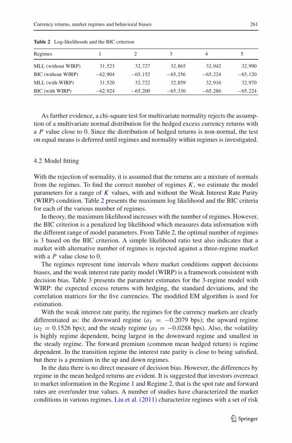
With the rejection of normality, it is assumed that the returns are a mixture of normalsfrom the regimes. To find the correct number of regimes K , we estimate the modelparameters for a range of K values, with and without the Weak Interest Rate Parity(WIRP) condition. Table 2 presents the maximum log likelihood and the BIC criteriafor each of the various number of regimes.

In theory, the maximum likelihood increases with the number of regimes. However,the BIC criterion is a penalized log likelihood which measures data information withthe different range of model parameters. From Table 2, the optimal number of regimesis 3 based on the BIC criterion. A simple likelihood ratio test also indicates that amarket with alternative number of regimes is rejected against a three-regime marketwith a P value close to 0.

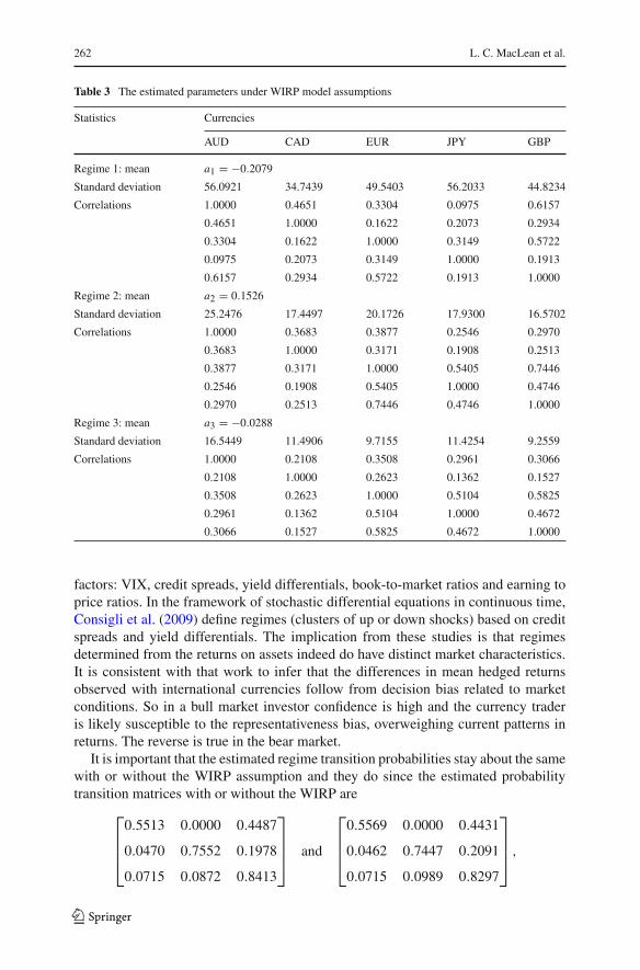
The regimes represent time intervals where market conditions support decisionsbiases, and the weak interest rate parity model (WIRP) is a framework consistent withdecision bias. Table 3 presents the parameter estimates for the 3-regime model withWIRP: the expected excess returns with hedging, the standard deviations, and thecorrelation matrices for the five currencies. The modified EM algorithm is used forestimation.

With the weak interest rate parity, the regimes for the currency markets are clearlydifferentiated as: the downward regime (a1 = −0.2079 bps); the upward regime(a2 = 0.1526 bps); and the steady regime (a3 = −0.0288 bps). Also, the volatilityis highly regime dependent, being largest in the downward regime and smallest inthe steady regime. The forward premium (common mean hedged return) is regimedependent. In the transition regime the interest rate parity is close to being satisfied,but there is a premium in the up and down regimes.

In the data there is no direct measure of decision bias. However, the differences byregime in the mean hedged returns are evident. It is suggested that investors overreactto market information in the Regime 1 and Regime 2, that is the spot rate and forwardrates are over/under true values. A number of studies have characterized the marketconditions in various regimes. Liu et al. (2011) characterize regimes with a set of risk

123


Table 3 The estimated parameters under WIRP model assumptions

Statistics Currencies

AUD CAD EUR JPY GBP

Regime 1: mean a1 = −0.2079


Correlations 1.0000 0.4651 0.3304 0.0975 0.6157

0.4651 1.0000 0.1622 0.2073 0.2934

0.3304 0.1622 1.0000 0.3149 0.5722

0.0975 0.2073 0.3149 1.0000 0.1913

0.6157 0.2934 0.5722 0.1913 1.0000

Regime 2: mean a2 = 0.1526


Correlations 1.0000 0.3683 0.3877 0.2546 0.2970

0.3683 1.0000 0.3171 0.1908 0.2513

0.3877 0.3171 1.0000 0.5405 0.7446

0.2546 0.1908 0.5405 1.0000 0.4746

0.2970 0.2513 0.7446 0.4746 1.0000

Regime 3: mean a3 = −0.0288


Correlations 1.0000 0.2108 0.3508 0.2961 0.3066

0.2108 1.0000 0.2623 0.1362 0.1527

0.3508 0.2623 1.0000 0.5104 0.5825

0.2961 0.1362 0.5104 1.0000 0.4672

0.3066 0.1527 0.5825 0.4672 1.0000

factors: VIX, credit spreads, yield differentials, book-to-market ratios and earning toprice ratios. In the framework of stochastic differential equations in continuous time,Consigli et al. (2009) define regimes (clusters of up or down shocks) based on creditspreads and yield differentials. The implication from these studies is that regimesdetermined from the returns on assets indeed do have distinct market characteristics.It is consistent with that work to infer that the differences in mean hedged returnsobserved with international currencies follow from decision bias related to marketconditions. So in a bull market investor confidence is high and the currency traderis likely susceptible to the representativeness bias, overweighing current patterns inreturns. The reverse is true in the bear market.

It is important that the estimated regime transition probabilities stay about the samewith or without the WIRP assumption and they do since the estimated probabilitytransition matrices with or without the WIRP are

⎡

⎢⎢⎣

0.5513 0.0000 0.4487

0.0470 0.7552 0.1978

0.0715 0.0872 0.8413

⎤

⎥⎥⎦ and

⎡

⎢⎢⎣

0.5569 0.0000 0.4431

0.0462 0.7447 0.2091

0.0715 0.0989 0.8297

⎤

⎥⎥⎦ ,

123


respectively. The regime transition matrices are very close, reinforcing our predictionabout regimes being independent of interest rate parity.

The estimated transition matrices are diagonal dominant, supporting the persistenceof regimes in the market dynamics. The probability of switching from the upwardto downward regimes without going through the steady regime is negligible. Thedata (hedged returns) imply periods of time (regimes) where currency traders over-shoot/undershoot spot rates and forward rates.

4.3 Weak interest rate parity tests

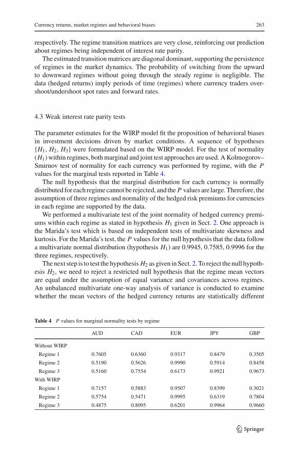
The parameter estimates for the WIRP model fit the proposition of behavioral biasesin investment decisions driven by market conditions. A sequence of hypotheses{H1, H2, H3} were formulated based on the WIRP model. For the test of normality(H1) within regimes, both marginal and joint test approaches are used. A Kolmogorov–Smirnov test of normality for each currency was performed by regime, with the Pvalues for the marginal tests reported in Table 4.

The null hypothesis that the marginal distribution for each currency is normallydistributed for each regime cannot be rejected, and the P values are large. Therefore, theassumption of three regimes and normality of the hedged risk premiums for currenciesin each regime are supported by the data.

We performed a multivariate test of the joint normality of hedged currency premi-ums within each regime as stated in hypothesis H1 given in Sect. 2. One approach isthe Marida’s test which is based on independent tests of multivariate skewness andkurtosis. For the Marida’s test, the P values for the null hypothesis that the data followa multivariate normal distribution (hypothesis H1) are 0.9945, 0.7585, 0.9996 for thethree regimes, respectively.

The next step is to test the hypothesis H2 as given in Sect. 2. To reject the null hypoth-esis H2, we need to reject a restricted null hypothesis that the regime mean vectorsare equal under the assumption of equal variance and covariances across regimes.An unbalanced multivariate one-way analysis of variance is conducted to examinewhether the mean vectors of the hedged currency returns are statistically different

Table 4 P values for marginal normality tests by regime

AUD CAD EUR JPY GBP

Without WIRP

Regime 1 0.7605 0.6360 0.9317 0.8479 0.3505

Regime 2 0.5190 0.5626 0.9990 0.5914 0.8458

Regime 3 0.5160 0.7554 0.6173 0.9921 0.9673

With WIRP

Regime 1 0.7157 0.5883 0.9507 0.8399 0.3021

Regime 2 0.5754 0.5471 0.9995 0.6319 0.7804

Regime 3 0.4875 0.8095 0.6201 0.9964 0.9660

123


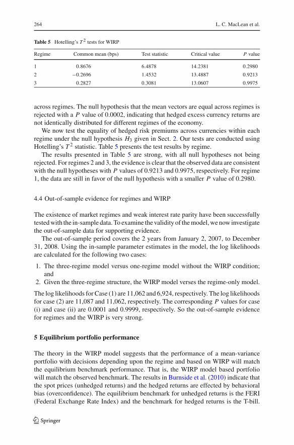
Table 5 Hotelling’s T 2 tests for WIRP

Regime Common mean (bps) Test statistic Critical value P value

1 0.8676 6.4878 14.2381 0.2980

2 −0.2696 1.4532 13.4887 0.9213

3 0.2827 0.3081 13.0607 0.9975

across regimes. The null hypothesis that the mean vectors are equal across regimes isrejected with a P value of 0.0002, indicating that hedged excess currency returns arenot identically distributed for different regimes of the economy.

We now test the equality of hedged risk premiums across currencies within eachregime under the null hypothesis H3 given in Sect. 2. Our tests are conducted usingHotelling’s T 2 statistic. Table 5 presents the test results by regime.

The results presented in Table 5 are strong, with all null hypotheses not beingrejected. For regimes 2 and 3, the evidence is clear that the observed data are consistentwith the null hypotheses with P values of 0.9213 and 0.9975, respectively. For regime1, the data are still in favor of the null hypothesis with a smaller P value of 0.2980.

4.4 Out-of-sample evidence for regimes and WIRP

The existence of market regimes and weak interest rate parity have been successfullytested with the in-sample data. To examine the validity of the model, we now investigatethe out-of-sample data for supporting evidence.

The out-of-sample period covers the 2 years from January 2, 2007, to December31, 2008. Using the in-sample parameter estimates in the model, the log likelihoodsare calculated for the following two cases:

1. The three-regime model versus one-regime model without the WIRP condition;and

2. Given the three-regime structure, the WIRP model verses the regime-only model.

The log likelihoods for Case (1) are 11,062 and 6,924, respectively. The log likelihoodsfor case (2) are 11,087 and 11,062, respectively. The corresponding P values for case(i) and case (ii) are 0.0001 and 0.9999, respectively. So the out-of-sample evidencefor regimes and the WIRP is very strong.

5 Equilibrium portfolio performance

The theory in the WIRP model suggests that the performance of a mean-varianceportfolio with decisions depending upon the regime and based on WIRP will matchthe equilibrium benchmark performance. That is, the WIRP model based portfoliowill match the observed benchmark. The results in Burnside et al. (2010) indicate thatthe spot prices (unhedged returns) and the hedged returns are effected by behavioralbias (overconfidence). The equilibrium benchmark for unhedged returns is the FERI(Federal Exchange Rate Index) and the benchmark for hedged returns is the T-bill.

123


The FERI is based on actual trading and will include decision bias (if it exists). Therates on T-bills do not respond as quickly to market conditions and it is possible thatthere is some deviation from the hedged model portfolio.

5.1 Portfolio performance: in sample

We now analyze the equilibrium implications of the assumptions on regimes and theweak interest rate parity for the currency market with in sample data. The equilibriumportfolio is calculated from Eq. (10) . For comparison mean-variance portfolios arealso calculated for alternative models: regimes but no WIRP; no regimes. The optimalmean-variance portfolio weights in each regime with the weak interest rate parity, theoptimal portfolio weights in each regime without weak interest rate parity, and thestatic mean-variance efficient portfolio are reported in Table 6.

The optimal portfolio weights vary substantially with different assumptions con-cerning the dynamics of the exchange rates. The phenomena of high leverages forboth the static mean-variance portfolio and the portfolio with regimes but withoutWIRP do not produce reasonable portfolio weights. The static mean-variance analysisassumes normality for currency returns, which is not true for the five currencies. Allow-ing for regimes without WIRP also presents portfolio weights incompatible with themarket equilibrium portfolio. However, the reasonable portfolio weights for the caseof regimes and WIRP are comparable with expectations for the market equilibriumportfolio and provide strong evidence for the parity condition to hold. The portfolioperformances will further reinforce this observation.

In order to quantify portfolio comparisons, the root mean square error is used tomeasure the average performance for the study period of a portfolio over a presetbenchmark. Denote by P̃t the cumulative return on the portfolio and by B̃t the cumu-lative return on a benchmark up to time t . The root mean square error of a portfoliorelative to the benchmark, Δ̃p, is presented in Table 7.

The weak interest rate parity model is supported by the currency data. The com-parisons of performance in both the in-sample and the out of sample data show thatthe presence of regimes and the weak interest rate assumptions are appropriate. With

Table 6 Optimal hedged portfolio weights

Model assumptions AUD CAD EUR JPY GBP

With WIRP

Regime 1 −0.0400 0.5491 0.1274 0.1417 0.2218

Regime 2 0.0255 0.4220 −0.0092 0.2330 0.3287

Regime 3 0.0143 0.3876 0.1095 0.1826 0.3059

Without WIRP

Regime 1 −12.2966 −1.9380 11.7061 24.8610 −21.3325

Regime 2 1.7996 −0.8072 −0.7829 −3.0884 3.8790

Regime 3 53.4417 12.8542 −95.4847 −157.4005 187.5892

Static mean-variance 4.5165 −0.3364 −4.0097 −9.7429 10.5724

123


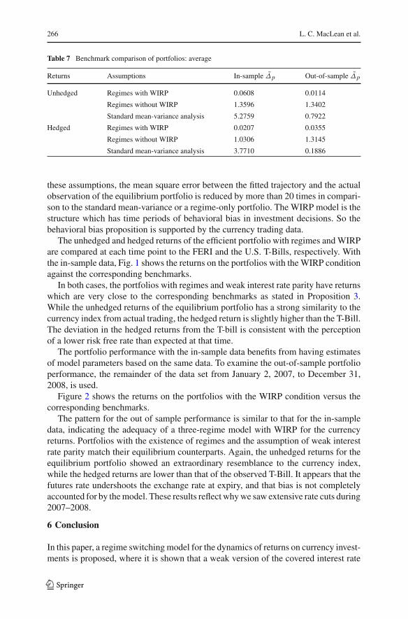
Table 7 Benchmark comparison of portfolios: average

Returns Assumptions In-sample Δ̃p Out-of-sample Δ̃p

Unhedged Regimes with WIRP 0.0608 0.0114

Regimes without WIRP 1.3596 1.3402

Standard mean-variance analysis 5.2759 0.7922

Hedged Regimes with WIRP 0.0207 0.0355

Regimes without WIRP 1.0306 1.3145

Standard mean-variance analysis 3.7710 0.1886

these assumptions, the mean square error between the fitted trajectory and the actualobservation of the equilibrium portfolio is reduced by more than 20 times in compari-son to the standard mean-variance or a regime-only portfolio. The WIRP model is thestructure which has time periods of behavioral bias in investment decisions. So thebehavioral bias proposition is supported by the currency trading data.

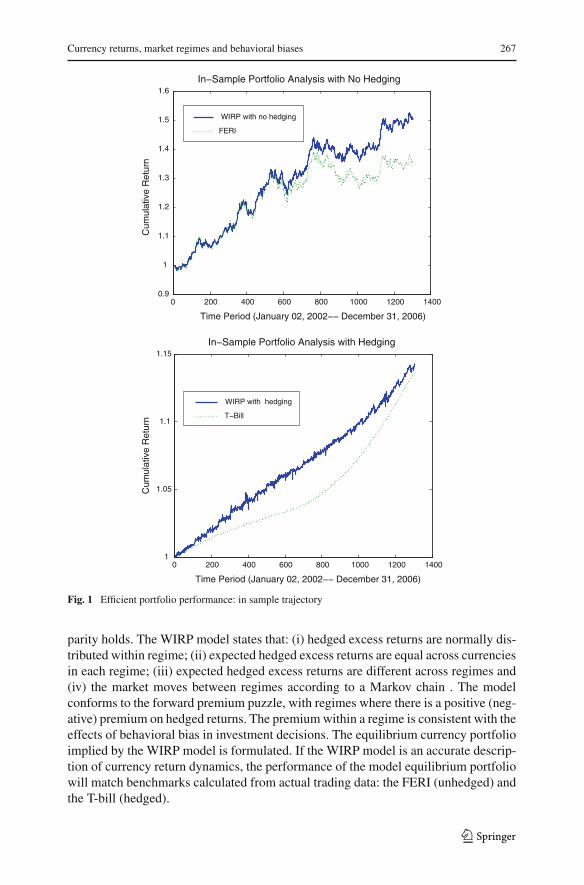
The unhedged and hedged returns of the efficient portfolio with regimes and WIRPare compared at each time point to the FERI and the U.S. T-Bills, respectively. Withthe in-sample data, Fig. 1 shows the returns on the portfolios with the WIRP conditionagainst the corresponding benchmarks.

In both cases, the portfolios with regimes and weak interest rate parity have returnswhich are very close to the corresponding benchmarks as stated in Proposition 3.While the unhedged returns of the equilibrium portfolio has a strong similarity to thecurrency index from actual trading, the hedged return is slightly higher than the T-Bill.The deviation in the hedged returns from the T-bill is consistent with the perceptionof a lower risk free rate than expected at that time.

The portfolio performance with the in-sample data benefits from having estimatesof model parameters based on the same data. To examine the out-of-sample portfolioperformance, the remainder of the data set from January 2, 2007, to December 31,2008, is used.

Figure 2 shows the returns on the portfolios with the WIRP condition versus thecorresponding benchmarks.

The pattern for the out of sample performance is similar to that for the in-sampledata, indicating the adequacy of a three-regime model with WIRP for the currencyreturns. Portfolios with the existence of regimes and the assumption of weak interestrate parity match their equilibrium counterparts. Again, the unhedged returns for theequilibrium portfolio showed an extraordinary resemblance to the currency index,while the hedged returns are lower than that of the observed T-Bill. It appears that thefutures rate undershoots the exchange rate at expiry, and that bias is not completelyaccounted for by the model. These results reflect why we saw extensive rate cuts during2007–2008.

6 Conclusion

In this paper, a regime switching model for the dynamics of returns on currency invest-ments is proposed, where it is shown that a weak version of the covered interest rate

123


0 200 400 600 800 1000 1200 14000.9

1

1.1

1.2

1.3

1.4

1.5

1.6

Time Period (January 02, 2002−− December 31, 2006)

Cum

ulat

ive

Ret

urn

In−Sample Portfolio Analysis with No Hedging

WIRP with no hedging

FERI

0 200 400 600 800 1000 1200 14001

1.05

1.1

1.15


Cum

ulat

ive

Ret

urn

In−Sample Portfolio Analysis with Hedging

WIRP with hedging

T−Bill

Fig. 1 Efficient portfolio performance: in sample trajectory

parity holds. The WIRP model states that: (i) hedged excess returns are normally dis-tributed within regime; (ii) expected hedged excess returns are equal across currenciesin each regime; (iii) expected hedged excess returns are different across regimes and(iv) the market moves between regimes according to a Markov chain . The modelconforms to the forward premium puzzle, with regimes where there is a positive (neg-ative) premium on hedged returns. The premium within a regime is consistent with theeffects of behavioral bias in investment decisions. The equilibrium currency portfolioimplied by the WIRP model is formulated. If the WIRP model is an accurate descrip-tion of currency return dynamics, the performance of the model equilibrium portfoliowill match benchmarks calculated from actual trading data: the FERI (unhedged) andthe T-bill (hedged).

123


0 100 200 300 400 500 6000.9

0.95

1

1.05

1.1

1.15

1.2

1.25


Cum

ulat

ive

Ret

urn

Out−Of−−Sample Portfolio Analysis with No Hedging

WIRP with hedging

FERI

0 100 200 300 400 500 6000.98

1

1.02

1.04

1.06

1.08

1.1


Cum

ulat

ive

Ret

urn

Out−Of−−Sample Portfolio Analysis with Hedging

WIRP with hedging

T−Bill

Fig. 2 Efficient portfolio performance: out of sample trajectory

A three-regime WIRP model was fitted to international currency data for the years2002–2008. To test the validity of the model, a series of in-sample and out-of-sampletests were performed. The regime-dependent mean-variance efficient portfolios werecompared with benchmark equilibrium portfolios. There is strong statistical evidencesupporting the hypotheses underlying the WIRP model.

A number of conclusions are drawn from the analysis. (i) There is direct evidence ofthe existence of regimes in the currency market, with a weak form of interest rate parity.The mean hedged returns have a positive (negative) premium depending on the marketregime and this is indirect evidence of a representativeness bias in decision making.(ii) The dynamics of regime switching are reasonably persistent in the sense thathistorical estimates of transition probabilities predict future regimes of the economy.

123


(iii) The performance of MV portfolios formed on the basis of the WIRP model isa close match to the performance of observed equilibrium portfolios both with andwithout hedging. (iv) The results on portfolio performance with regime switching haveimportant implications for the equilibrium allocation of investments. The currencyportfolio may be part of a larger portfolio of international assets. However, the accurateestimates for currency returns are an important factor in valuing international assets.If the assessment of foreign exchange exposures is in error, this increases the risk withinternational portfolios. A currency overlay strategy based on estimated parameters inthe WIRP model should reduce the risk from currency exposures.

References

Akram, Q., Rime, D., Sarno, L.: Arbitrage in the foreign exchange market: turning on the microscope. J IntEcon 76(2), 237–253 (2008)

Ang, A., Bekaert, G.: International asset allocation with regime shifts. Rev Financ Stud 15, 1137–1187(2002)

Bansal, R.: An exploration of the forward premium puzzle in currency markets. Rev Financ Stud 10,369–403 (1997)

Baz, J., Breedon, F., Naik, V., Peress, J.: Optimal portfolios of foreign currencies. J Portf Manag 28, 102–110(2001)

Bekaert, G., Hodrick, R.J.: On the biases in the measurement of foreign exchange risk premiums. J IntMoney Financ 12, 115–138 (1993)

Biasis, B., Hilton, D., Mazurier, K., Pouget, S.: Judgemental overconfidence, self-monitoring, and tradingperformance in an experimental financial market. Rev Econ Stud 72, 287–312 (2005)

Burnside, C., Han, B., Hirshleifer, D., Wang, T.: Investor overconfidence and the forward premium puzzle.Rev Econ Stud 78, 523–558 (2010)

Consigli, G., MacLean, L., Zhao, Y., Ziemba, W.: The bond-stock yield differential as a risk indicator infinancial markets. J Risk 13, 1–22 (2009)

De Santis, G., Gerard, B.: International asset pricing and portfolio diversification with time-varying risk. JFinanc 52, 1881–1912 (1997)

Dempster, A.P., Laird, N.M., Rubin, D.B.: Maximum likelihood from incomplete data via the EM algorithm.J R Stat Soc (Ser B) 39, 1–38 (1977)

Erb, C.B., Harvey, C.R., Viskanta, T.E.: Forecasting international equity correlations. Financ Anal J 50,32–45 (1994)

Fuller, R.J.: Behavioral finance and the sources of alpha. J Pension Plan Invest 2, 1–21 (1998)Hanoch, G., Levy, H.: The efficiency analysis of choices involving risk. Review of Economic Studies 36(3),

335–346 (1969)Kahneman, D., Tversky, A.: Prospect theory: an analysis of decision making under risk. Econometrica 47,

263–291 (1979)Liu, P., Xu, K., Zhao, Y.: Market regimes, sectorial investment, and time-varying risk premiums. Int J Manag

Financ 7, 107–133 (2011)Longin, F., Solnik, B.: Is the correlation in international equity returns constant: 1960–1990? J Int Money

Financ 14, 3–26 (1995)Longin, F., Solnik, B.: Correlation structure of international equity markets during extremely volatile peri-

ods. J Financ 56, 649–676 (2001)Marida, K.: Tests of univariate and multivariate normality. In: Handbook of Statistics, vol. 1, S.Kotz et al.

(eds). pp. 279–320. New York: Wiley (1980)Schwarz, G.E.: Estimating the dimension of a model. Ann Stat 6, 461–464 (1978)Xia, Y.: Learning about predictability: the effects of parameter uncertainty on dynamic asset allocation.

J Financ 56, 205–246 (2001)

123

currency returns, market regimes and behavioral biases

Documents