cure information svnc

1

UNDERSTANDING CURE WITH THESCANNING VIBRATING NEEDLE CUREMETER

(SCANNING VNC)(RTL/2844)

Authors: B.G. Willoughby and K.W. Scott

Rapra Technology Limited,Shawbury,

Shrewsbury,Shropshire.SY4 4NR.

Tel. +44 (0)1939 250383Fax. +44 (0)1939 251118

SVNC Cure MonitoringRTL/2844

1

CONTENTS

1. INTRODUCTION....................................................................................................... 12. MONITORING LIQUID POLYMER CURES............................................................ 3

2.1 Elasticity and Modulus .................................................................................... 32.2 Modulus and Cure............................................................................................ 32.3 Fluid Flow and Viscosity .................................................................................. 42.4 Oscillatory Measurements................................................................................. 52.5 Phase Angle (δ) ................................................................................................ 82.6 Summary of Changes During Cure ................................................................... 152.7 Practical Cure Monitoring - The Rapra Scanning VNC..................................... 15

2.7.1 The Instrument................................................................................ 162.7.2 Amplitude Attenuation for the Scanning VNC................................. 192.7.3 Resonance Frequency Effects .......................................................... 26

2.8 References........................................................................................................ 303. MONITORING THE CURE OF THERMOSET RESINS WITH THESCANNING VNC............................................................................................................. 31

3.1 Polyurethanes................................................................................................... 333.2 Polysulphides ................................................................................................... 353.3 Silicones........................................................................................................... 363.4 Epoxy Cures .................................................................................................... 363.5 Unsaturated Polyester Resins............................................................................ 373.6 Visible Light Cure ........................................................................................... 383.7 PVC Plastisols.................................................................................................. 383.8 Polyurethane Foams ......................................................................................... 403.9 Cure Monitoring of Thin Films ......................................................................... 453.10 Comparison of Fixed Frequency Monitoring and ScanningFrequency Monitoring............................................................................................ 453.11 Assessment of Cured Rubbers ....................................................................... 473.12 Summary....................................................................................................... 483.13 References..................................................................................................... 48

INDEX ............................................................................................................................. 49


1

UNDERSTANDING CURE WITH THE SCANNING VIBRATING NEEDLECUREMETER (SCANNING VNC)

1. INTRODUCTION

The Scanning Vibrating Needle Curemeter (SVNC) is a simple and robust instrumentwhich is capable of providing a continuous profile of liquid polymer cures:

- for elastomeric systems up to the final stages of cure;

- for glassy systems, approaching the point of vitrification.

A continuous profile provides new levels of discrimination, releasing the technologistfrom the constraints of single point determinations. No longer need "gel point" be thesole focus of attention - a point in practical terms too long to define the working life ofthe uncured mix but too short to define demould time. Figure 1 shows the kind of

output obtained.There are twocontinuous cureprofiles givingcomplimentaryinformation. Whatthey mean withrespect to thedevelopment of cureis discussed in moredetail in Section 2 ofthis document.

Examples covering a diversity of cure profiles for cure systems are given Section 3.All the examples are also provided as data files on the SVNC Program disk(Version 2.2) and can be displayed using the SVNC software - see "Operating Manualfor the ScanningVNC" RTL/2843, Sections 5.5, 6.1.1.1 and 6.3 or "Description of aDemonstration Program for the Scanning Vibrating Needle Curemeter (ScanningVNC)" RTL/2846, Sections 4.1.1 and 4.2.

What is shown in Figure 1 are two outputs covering elastic (solid line) and dampingresponses. Together they show how fast cure is developing and what kind of productis obtained. They enable practical concepts of application time, work life, demouldtime, etc., to be put into a coherent and recordable context.


2

In fact the standard software supplied with the SVNC allows for eighteen diagnosticpoints (including gel time) to be allocated for comparative purposes. Some can beselected entirely at the discretion of the user.

Reference to the "standard software" highlights a key feature of the SVNC in that it isa computer driven instrument - indeed the reader will soon realise it is only possible tooperate this device in computer driven form. The sampling head is simple and robust -the sophistication is in the control. Yet developments in computers allow this controlto be achieved with nothing more elaborate than a modern PC (386 or faster). Oncethe standard software is loaded, any IBM compatible PC of sufficient power can drivethe SVNC. The control panel is even a display on the screen.

Integrating a computer into an instrument in this way obviates the need for a dedicatedchart recorder - or for the storage and archiving of chart material. All recorded curetraces can be stored, and retrieved, as computer files. New data can be compared withold data directly on screen. Of course hard copies can be produced, as required, usingconventional printers. Detail of the operation of the instrument are given inRTL/2843.


3

2. MONITORING LIQUID POLYMER CURES

During the cure of a liquid polymer, chain extension and crosslinking processes causechanges in the viscous and elastic properties of the polymer. Liquids which cure tosolids are of major technological importance, providing structural materials(e.g. GRP), solid and foamed rubbers (e.g. PU, silicones), surface coatings andadhesives. Thus the reliable monitoring of these production processes is vital toeffective process and product control, yet often little may be done bar a cursory singlepoint determination (gel point). Whilst the technologist may recognise the importanceof optimising application time, work life, etc., profiling cures has not reached thewidespread acceptance that is seen in solid rubber processing.

The problem may reflect the major changes taking place with liquid polymer cures.These changes not only extend beyond the dynamic ranges of many measurementdevices, they also challenge the technologist with respect to their understanding andrationalisation. Those seeking an up-to-date summary of network theory shouldconsult Dusek1 and the references listed therein.

However, familiarity with modern branching theory is not a pre-requisite to theunderstanding of liquid polymer cures, nor is access to expensive instrumentation apre-requisite to monitoring them. This section explains in basic terms what changesare occurring during the cure and how the Scanning VNC can record them.

2.1 Elasticity and Modulus

A solid has a defined shape and an elastic solid is one which will revert to its originalshape after any imposed distortion has been removed. The characteristic resistance tosuch distortion is the stiffness, or “modulus”, of the material.

Over the region where a solid displays ideal elastic behaviour, the resulting strain (γ) isdirectly proportional to the imposed stress (σ). Hence for example in simple shear

σ = Gγ

where G is the shear modulus

2.2 Modulus and Cure

In rubbers, elastic behaviour results from a molecular architecture in which freelyjointed chains are linked together at certain points (crosslinks). The restoring forceagainst any imposed distortion arises from thermal motion and the drive to restore theequilibrium chain configuration. In the ideal elastic network where all molecular


4

segments can contribute to their restoring force (the so-called “Gaussian” condition),then shear modulus is directly proportional to crosslink density, i.e.

G = NkT

where N is the number of chains per unit vol.

K = Boltzmann’s constant

T = absolute temperature

Alternatively, if Mc is the molecular weight between crosslinks, then:

G = pRT/Mc

where p = material density

R = gas constant per mole

Although representative of an ideal case (freely-jointed chains, no network defects,etc.), the simplicity of the above relationship invites widespread use. Thus modulus isregarded as an index of “state of cure”; the cure being regarded as complete when themodulus has reached its maximum value and the faster that modulus increases, then thefaster is the cure. Given the inherent difficulty of measuring Mc directly, suchpragmatism is not unreasonable.

2.3 Fluid Flow and Viscosity

The molecular weights of segments in a network may present a severe challenge tomeasurement, but molecular weight per se is not beyond the scope of nominallyroutine investigation. For molecules of finite length, molecular weight is capable ofestimation by a variety of techniques. For liquid polymers, a growth in molecularweight is indicative of the onset of cure. This is reflected as an increase in viscosity,one theoretical treatment suggesting (for monodisperse polymers)

η α M3.5

where η is the coefficient of viscosity.

Whilst viscosity itself is amenable to convenient, and continuous, monitoring, it shouldbe recognised that the data obtained can give little insight into the processes ofcrosslinking. Viscosity is a property of a fluid, whilst molecular crosslinking is morecommonly associated with solid materials.

A fluid will flow whenever a stress is applied and continue to flow for as long as thatstress is in place. The resistance to flow is reflected in the rate of flow which results,and for an ideal (Newtonian) fluid the defining relationship is:


5

σ ηγ=

where σ is shear stress

and γ is the resulting shear rate

Thus if the coefficient of viscosity (η) is low, less stress will be required to maintain agiven shear rate, monitoring the torque required to achieve a given rotational shearrate being a common means of measuring η. What is obtained is a steady statecoefficient, and this value must become infinite if and when the transition to a solidoccurs.

This transition marks the point when a curing liquid is no longer capable of flow - i.e.the “gel point”. As an infinite value would be outside the measuring range ofconventional steady state (e.g. rotational) instruments, continuous monitoring ofsteady state viscosity up to the gel point is not feasible.

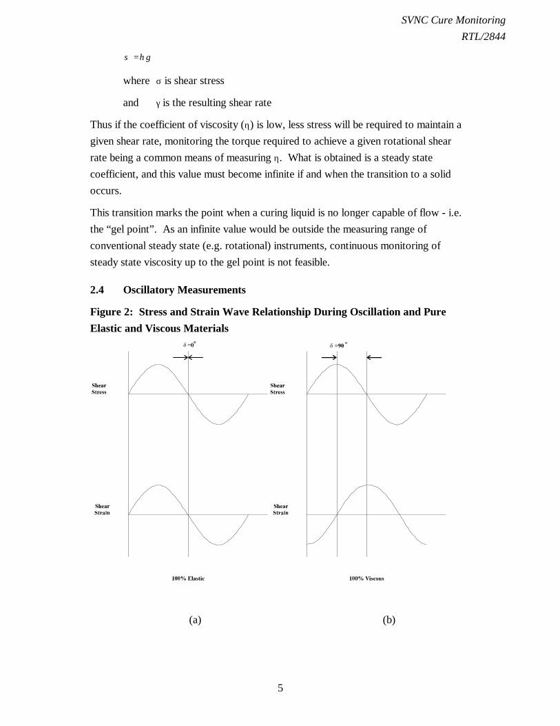
2.4 Oscillatory Measurements

Figure 2: Stress and Strain Wave Relationship During Oscillation and PureElastic and Viscous Materials

(a) (b)


6

For solid rubbers, the most commonly employed form of continuous cure monitoring isby an oscillatory or reciprocating technique. Thus instruments such as the Wallace-Shawbury Curometer and the Monsanto Rheometer have widespread familiarity.

The kind of information which can be obtained can be seen from the example of asinusoidal oscillation. The dependencies of stress and strain with time are shown inFigure 2(a): for a purely elastic solid, the maximum strain occurs at the point ofmaximum stress and the dependencies of stress and strain with time are completely inphase.

However this situation will not apply if the medium is purely viscous. Here themaximum stress produces the maximum rate of strain, and the dependencies of stressand strain with time are 90° out of phase (see Figure 2(b)). Thus for a purely viscousmaterial the strain lags the stress by 90°, the so-called phase angle (δ).

It follows that if a material is neither purely viscous nor purely elastic(i.e. visco-elastic), the sinusoidal stress and strain responses will not be in-phase, butthe phase angle will be less than 90°. The sinusoidal strain will lag behind the appliedstress; the stress (σ) and strain (γ) at any time t being given by the expressions

σ σ ω δγ γ ω

= +=

0

0

sin ( )

sin

t

t

where ω is the frequency

The equation for σ can be re-written

σ = σ ϖ δ σ ϖ δo osin t cos + t sincos

showing that the shear stress can be considered to consist of two parts: one which isin-phase with the strain (with an amplitude σ δo cos ) and the other which is 90°out-of-phase with the strain (with an amplitude σ δo sin ). The shear-stress/shear-strainrelationship can thus be specified by a modulus G' in-phase with the shear strain and amodulus G'' 90° out-of-phase with the strain, i.e.

′=Gσγ

δ0

0

cos

′′=Gσγ

δ0

0

sin

The parameters σ γo oand in the above expressions represent the amplitudes for thestress and strain waves, respectively. Thus if these, and the phase angle δ aredetermined experimentally, G' and G'' may be obtained.


7

An alternative mathematical treatment uses complex representations of stress andstrain, whereby:

( )σ σ ϖ δ*= oei t +

γ γ ω* = 0ei t

The complex modulus G* is given by:

( )G *= e cos + i sin*

*iσ

γσγ

σγ

δ δδ=

=

o

o

o

o

Hence

G* = G' + iG'

where G' is the in-phase or “storage” modulus

and G'' is the out-of-phase or “loss” modulus

Whereas the in-phase component relates to the elasticity in the material, the out-of-phase components relate to damping or viscous behaviour. Indeed, a complexviscosity can be derived from these values. Thus if the strain at any time t is given by:

γ γ ω* = 0ei t

Differentiating against time given:

&* *γ ωγ ωγω= =i e ii t0

Thus if G * =

σγ

**

η σγ ω

**

*

*

&= = G

i

Hence two complementary expressions can be derived:

G * = G + iG′ ′′

η η η* = ′− ′′i

and ′= ′′ ′′ ′η ηG / = G /w w

The dynamic viscosity coefficients are frequency-dependent parameters - at lowfrequencies ′η approaches the steady-state coefficient η, but its value remains finiteeven through gelation.


8

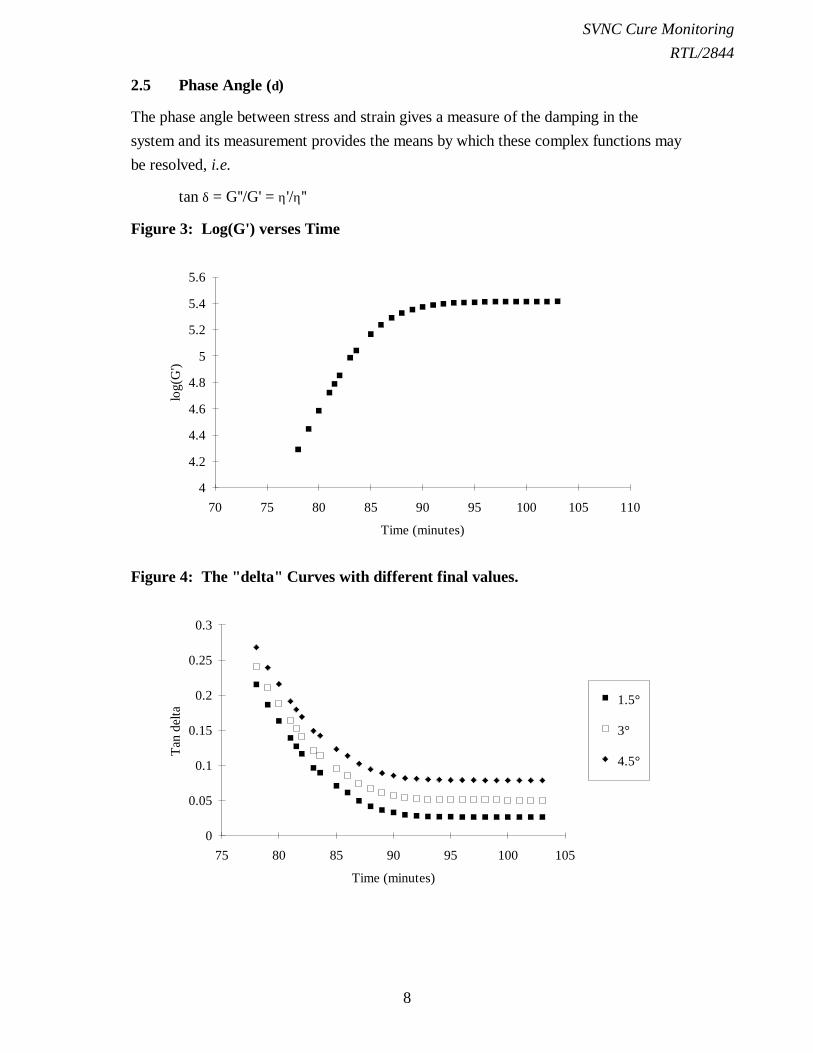
2.5 Phase Angle (δ)

The phase angle between stress and strain gives a measure of the damping in thesystem and its measurement provides the means by which these complex functions maybe resolved, i.e.

tan δ = G''/G' = η'/η''

Figure 3: Log(G') verses Time

Time (minutes)

log(

G')

4

4.2

4.4

4.6

4.8

5

5.2

5.4

5.6

70 75 80 85 90 95 100 105 110

Figure 4: The "delta" Curves with different final values.

Time (minutes)

Tan

delta

0

0.05

0.1

0.15

0.2

0.25

0.3

75 80 85 90 95 100 105

1.5°

3°

4.5°


9

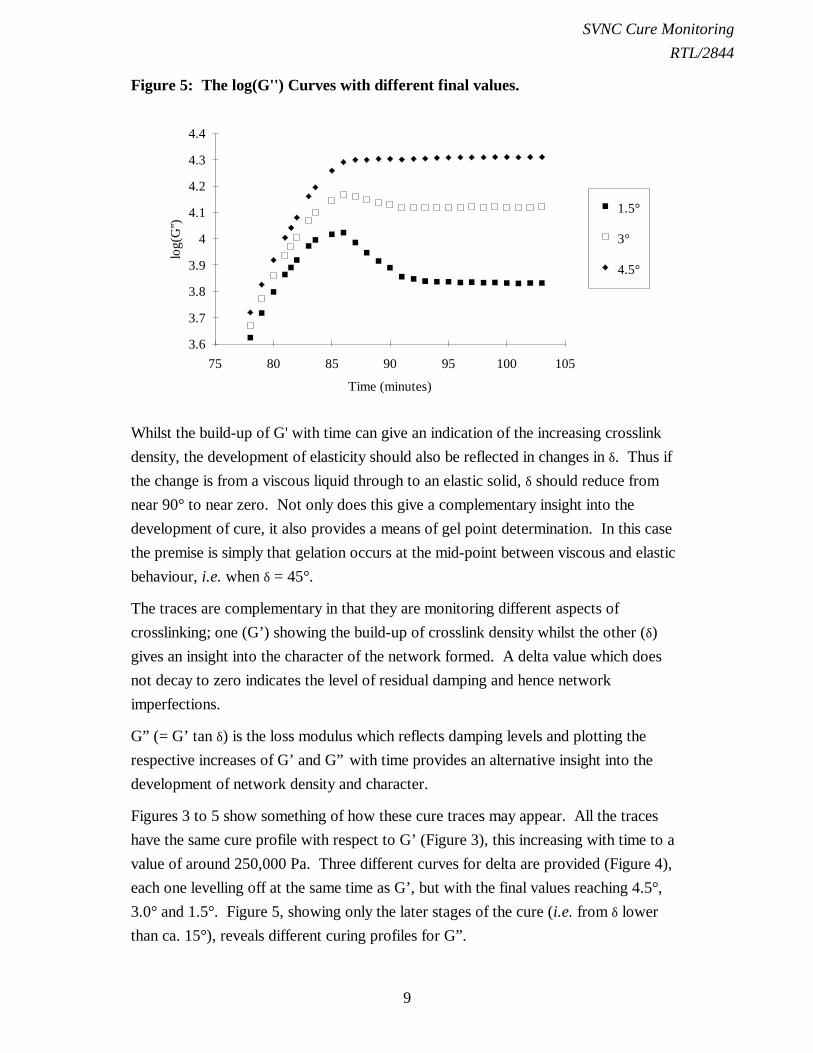
Figure 5: The log(G'') Curves with different final values.

Time (minutes)

log(

G'')

3.6

3.7

3.8

3.9

4

4.1

4.2

4.3

4.4

75 80 85 90 95 100 105

1.5°

3°

4.5°

Whilst the build-up of G' with time can give an indication of the increasing crosslinkdensity, the development of elasticity should also be reflected in changes in δ. Thus ifthe change is from a viscous liquid through to an elastic solid, δ should reduce fromnear 90° to near zero. Not only does this give a complementary insight into thedevelopment of cure, it also provides a means of gel point determination. In this casethe premise is simply that gelation occurs at the mid-point between viscous and elasticbehaviour, i.e. when δ = 45°.

The traces are complementary in that they are monitoring different aspects ofcrosslinking; one (G’) showing the build-up of crosslink density whilst the other (δ)gives an insight into the character of the network formed. A delta value which doesnot decay to zero indicates the level of residual damping and hence networkimperfections.

G” (= G’ tan δ) is the loss modulus which reflects damping levels and plotting therespective increases of G’ and G” with time provides an alternative insight into thedevelopment of network density and character.

Figures 3 to 5 show something of how these cure traces may appear. All the traceshave the same cure profile with respect to G’ (Figure 3), this increasing with time to avalue of around 250,000 Pa. Three different curves for delta are provided (Figure 4),each one levelling off at the same time as G’, but with the final values reaching 4.5°,3.0° and 1.5°. Figure 5, showing only the later stages of the cure (i.e. from δ lowerthan ca. 15°), reveals different curing profiles for G”.


10

The cure that leaves the highest level of residual damping (δ = 4.5°) shows G” rise to aplateau at around 20,000 Pa. When δ drops to 2.5°, the plateau value of G” issomewhat lower at around 13,500 Pa., but there are signs of an intermediate maximumvalue (at around 85 minutes) perhaps some 1,500 Pa. higher. The existence of anintermediate maximum is quite distinct in the third trace where δ drops to 1.5°. Herethe maximum is reached perhaps a little earlier than before and at a lower level of11,000 Pa. The residual plateau value is only 7,000 Pa.

These traces demonstrate pictorially what is in essence a mathematical expectation,namely that the product G' tan δ will be numerically low when either G' or tan δ arelow - i.e. at the start and end of cures. Thus the intermediate values of G'' may behigher than either starting or finishing values.

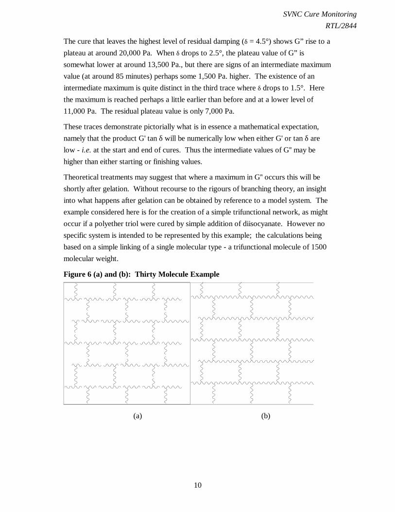
Theoretical treatments may suggest that where a maximum in G'' occurs this will beshortly after gelation. Without recourse to the rigours of branching theory, an insightinto what happens after gelation can be obtained by reference to a model system. Theexample considered here is for the creation of a simple trifunctional network, as mightoccur if a polyether triol were cured by simple addition of diisocyanate. However nospecific system is intended to be represented by this example; the calculations beingbased on a simple linking of a single molecular type - a trifunctional molecule of 1500molecular weight.

Figure 6 (a) and (b): Thirty Molecule Example

(a) (b)


11

Figure 6 (c): Thirty Molecule Example

(c)

Consider the example of 30 such molecules arranged in a suitable manner for networkformation (see Figure 6(a)). After the first bond has been formed there will remain 29molecules. Hence after 29 bonds there will be only one molecule (MW 45,000) andthe maximum molecular weight has been attained. The situation where all reactantshave been linked together to form one complete molecule is representative of the gelpoint - in reality the point where the molecular weight becomes infinite.

The example under consideration shows what happens after gelation. The 30th bondmade (first one after “gelation”) cannot raise the molecular weight any higher, butintroduces one crosslink. The 31st bond gives a second crosslink, and so on. In thesituation represented in the Figure 6(b), a total of 37 bonds have formed (74 chainends reacted, 16 still free). A plot of MW and N (number of crosslinks) against bondnumber from 1 - 37 gives the type of plot which might be expected for viscosity(before gelation) and G’ (after gelation).

What is happening within the crosslinked structure can be seen by assembling thenetwork, step-by-step. Each link is assigned a number from 1 - 37 (left-to-right, top-to-bottom) and the bonds are assembled in random number order. The situation at the29th bond is shown in Figure 6(c). The remaining eight bonds are filled in thenumerical sequence: 35 (30th), 24 (31st), 8 (32nd), 34 (33rd), 10 (34th), 27 (35th), 20(36th) and 3 (37th).

The build-up of molecular weight, both within the network and outside the networkscan be seen in Table 1.


12

Table 1:

No. of BondsMade

Av. Mol.Wt.

No. ofX-links

MW inopen chain

MW innetwork

0 1,500 0 1,500 -1 1,550 0 1,550 -10 2,250 0 2,250 -20 4,500 0 4,500 -25 9,000 0 9,000 -26 11,250 0 11,250 -27 15,000 0 15,000 -28 22,500 0 22,500 -29 45,000 0 45,000 030 45,000 1 35,000 10,00031 45,000 2 28,000 17,00032 45,000 3 23,000 22,00033 45,000 4 19,000 26,00034 45,000 5 15,000 30,00035 45,000 6 14,000 31,00036 45,000 7 13,000 32,00037 45,000 8 10,000 35,000

It is clear from this the network is changing in character as it forms with the molecularweight within the network eventually exceeding that in free chains. If the respectiveproportions of material inside and outside the network reflects the level of damping inthe system then it is perhaps not surprising that G'' continues to increase beyond the gelpoint.

However it might also be expected that in the final stages of network formation,especially when most of the material is combined within the network, then G” mustultimately decrease. Under these circumstances, a maximum value for G” will be seen.

2.6 Summary of Changes During Cure

The following scheme generalises the various stages that occur during the cure of aliquid polymer.

1. Viscosity increase.

2. Development of elasticity - (e.g. through entanglements) - end of work life.

3. Gelation (viscosity → ∞ ) - no flow beyond this point

4. Crosslink density increases (G' increases) - rate of G' change equates to rateof cure.


13

5. Network flaws decrease - extra network content decreases, networkcontent increases.

- G'' reaches a maximum-G'' may then decrease as flaws disappear.

6. Crosslinking reaction cease

G' reaches a maximumG'' levels out.

7. Reversion?

- G' starts to decrease- G'' starts to increase.

2.7 Practical Cure Monitoring - The Rapra Scanning VNC

Classical rheometers can give cure traces as above for a range of materials, but are notnecessarily optimised for curing liquids. One limitation relates to the strict geometricrequirements for the accurate determination of G’. The geometry which is imposedwill be that which is required for the measurement range, and not necessarily thatwhich is of interest to the technologist. The most active liquid curing systems willexploit their exothermic behaviour to some degree in their cures so that thin filmstudies may not be totally relevant. Such studies may characterise the system, but notnecessarily its practical curing characteristics.

Furthermore, the “system” as such must be taken to the instrument, indeed it may haveto be mixed in close proximity to the instrument if the true start of cure coincides withthe start of mixing. Additionally it may be less than willing to leave the instrument if astrong adhesive cure results.

It follows from this that, if an instrument can be taken to the cure (rather than the otherway around), practical benefit would result. A transportable robust instrument whichposes no special geometric constraints on the sample would have remarkable versatilityfor the monitoring of liquid polymer cures. Thus rapidly curing liquids could bemonitored in the thicker sections more representative of practice, or even in the mixingcontainer itself. Without unnecessary geometric constraints, cures could be monitoredwithin a container large enough to allow for expansion or even in applications relatedconfigurations.

This is the rationale behind the development of the Rapra Vibrating Needle Curemeter(or VNC), an instrument which is robust and transportable to the sample. The only


14

special constraints are the need for access for the needle into the sample and thenecessary mains electricity supply. The heart of the instrument is a simple electrically-driven vibrator and its power to resolve a cure comes from the manner of itsintegration to a PC. The computer both selects the frequency for oscillation andanalyses the outputs. Thus, unlike a great many other instruments, the VNC does notwork at a single fixed frequency. The fact that the instrument is scanning a range offrequencies gives it the name Scanning VNC.

2.7.1 The Instrument

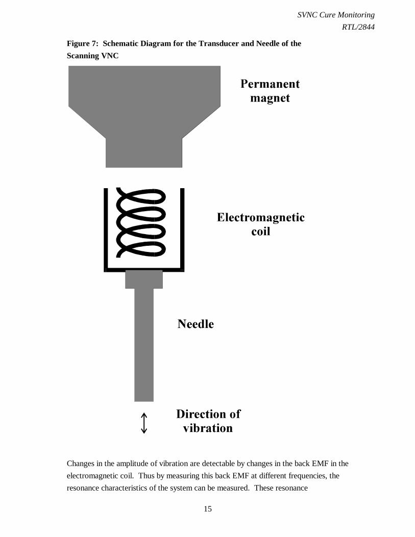
The heart of the Scanning VNC is the vibrator itself. This contains a moving coilassembly located via flexible mountings close to one pole of a permanent magnet(Figure 7). The coil is energised by an AC current to produce a vibration of the samefrequency as the oscillating current. This drive is provided by the Control Box of theinstrument and the frequency of the AC signal is scanned over a range of frequencies.


15

Figure 7: Schematic Diagram for the Transducer and Needle of theScanning VNC

Changes in the amplitude of vibration are detectable by changes in the back EMF in theelectromagnetic coil. Thus by measuring this back EMF at different frequencies, theresonance characteristics of the system can be measured. These resonance


16

characteristics, in particular the resonance frequency and amplitude, are used tomonitor the progress of cure.

2.7.2 Amplitude Attenuation for the Scanning VNC

The processes of cure will change the resonance characteristics of a vibrating probe(e.g. needle) penetrating that curing mix. How the resulting effects can be rationalisedrequires consideration of the whole system, then vibrator, the needle and the curingformulation.

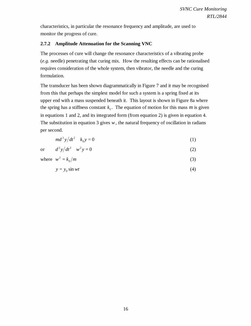
The transducer has been shown diagrammatically in Figure 7 and it may be recognisedfrom this that perhaps the simplest model for such a system is a spring fixed at itsupper end with a mass suspended beneath it. This layout is shown in Figure 8a wherethe spring has a stiffness constant k0. The equation of motion for this mass m is given

in equations 1 and 2, and its integrated form (from equation 2) is given in equation 4.The substitution in equation 3 gives ω , the natural frequency of oscillation in radiansper second.

md y dt k y2 20 0+ = (1)

or d y dt y2 2 2 0+ =ω (2)

where ω 20= k m (3)

y y t= 0 sin ω (4)


17

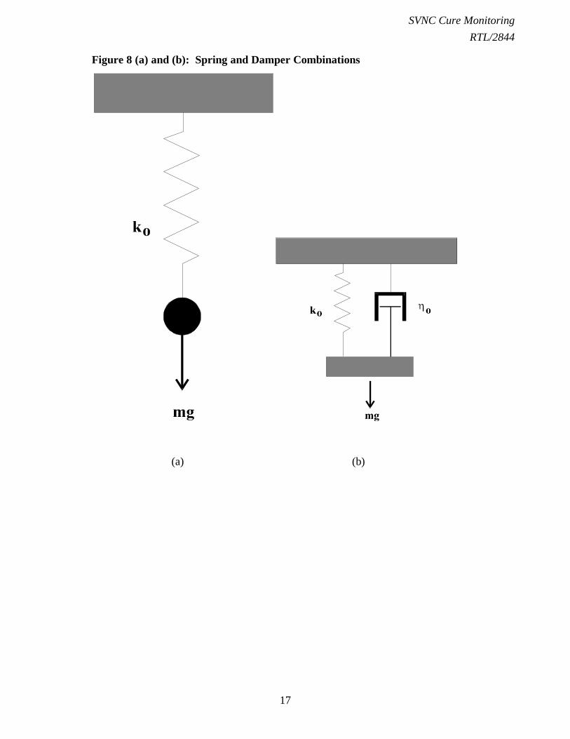
Figure 8 (a) and (b): Spring and Damper Combinations

(a) (b)


18

Figure 8 (c) and (d): Spring and Damper Combinations

(c) (d)

In free vibration, a system as described by this model vibrates at its natural frequency(ω = k m0 ). However in forced vibration, such a system is capable of oscillating at

any frequency as determined by the frequency of the periodic force. This is the case forthe electrodynamic transducer of the Scanning VNC where the vibration frequency isthat of the AC signal which energises the coil. However when the driving frequencyequals that of the natural frequency of the system the condition of resonance isobtained. This effect is readily seen with the Scanning VNC which with the standardvibrator and probe/needle gives a resonance peak (in air) at around 85 Hz.


19

In reality there will be some internal friction in the vibrator and a damping term shouldbe included in equations (1) and (2). The system is then represented by a spring anddash pot in parallel, as in Figure 8b.

This model is not representative of the situation when the vibration is being restrainedby an additional viscous element, as is the case when the VNC needle is in contact witha fluid. Figure 8c shows a modification to the first model to accommodate this, themass on the spring being immersed in a damping medium. This damping mediumrepresents the sample being monitored, the container for which should not itself be freeto vibrate. Thus the top and bottom of this system are both fixed in space with onlythe central part free to vibrate. Thus the layout in Figure 8c is equivalent to that inFigure 8d, the arrangement with the spring and dampers in parallel.

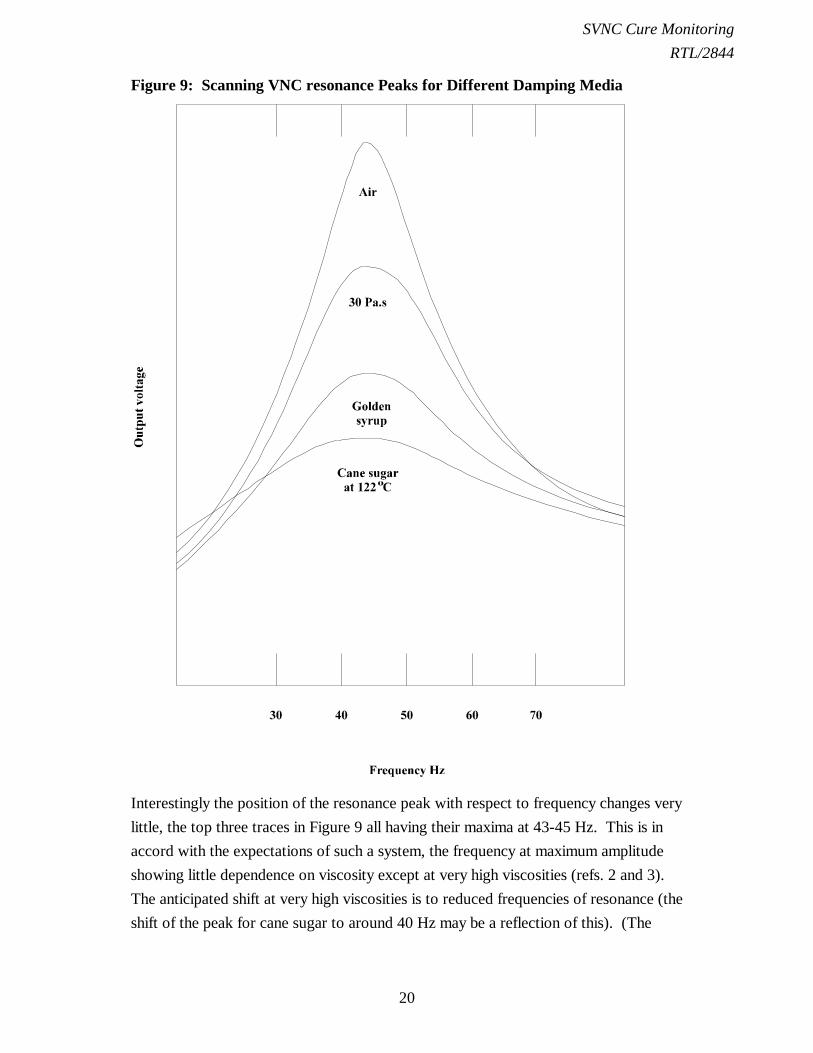
The effect of damping for forced vibrations is to reduce the amplitude. Figure 9 showsthis effect for the VNC at resonance in four different fluids: air, silicone oil, goldensyrup and molten sucrose (cane sugar). The amplitude at resonance as measured by theback EMF is significantly reduced as the viscosity increases to around 200 Pa.s in thecase of the cane sugar melt.


20

Figure 9: Scanning VNC resonance Peaks for Different Damping Media

Interestingly the position of the resonance peak with respect to frequency changes verylittle, the top three traces in Figure 9 all having their maxima at 43-45 Hz. This is inaccord with the expectations of such a system, the frequency at maximum amplitudeshowing little dependence on viscosity except at very high viscosities (refs. 2 and 3).The anticipated shift at very high viscosities is to reduced frequencies of resonance (theshift of the peak for cane sugar to around 40 Hz may be a reflection of this). (The


21

resonance frequencies are lower than usually obtained as the transducer used here wasnot the standard transducer.)

2.7.3 Resonance Frequency Effects

Gel time is an important parameter of the cure of liquid polymers and a usefulcure-monitoring device should be capable of recognising it. How this can be achievedwith the Scanning VNC may be appreciated by reference to the resonance peaksshown in Figure 10 measured during the cure of a polyurethane elastomer.

Figure 10: Typical Resonance Peaks for the Cure of a PU

Frequency (Hz)

Res

pons

e

0

1000

2000

3000

4000

5000

6000

7000

8000

9000

10000

0 50 100 150 200 250 300 350 400 450 500

What is evident is that the frequency of the resonance maximum is increasing, a featurenot observed in studies of purely viscous damping (e.g. see Figure 9). The reasons forthis may be appreciated by reference again to an elastic model.

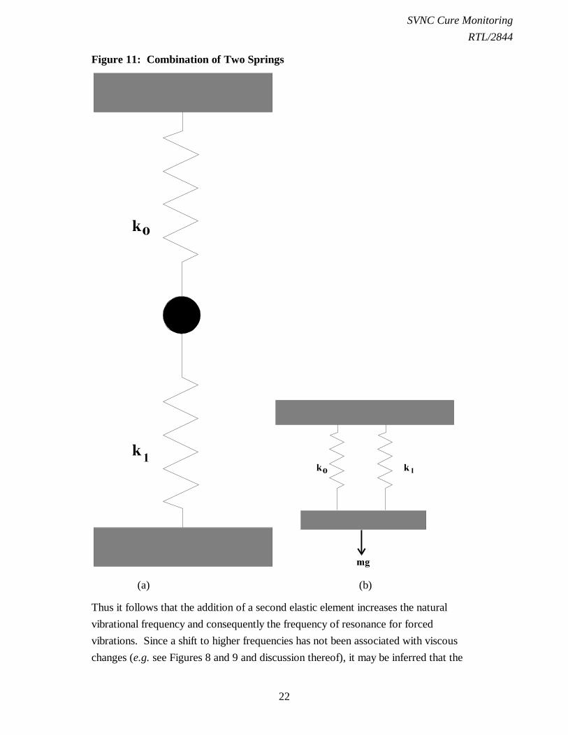
The change in resonance frequency for a model system can be illustrated with respectto the simplest of these, based on undamped springs as in Figure 8a. The introductionof a second spring beneath the vibrating mass is shown in the arrangement inFigure 11a where the second spring has a stiffness constant k1. If both springs act both

in extension and compression then the model is analogous to that in Figure 11b forwhich the equation of motion of the mass m is given by equation 5. It follows fromthis that the natural frequency for free vibration is given by the expression inequation 6.

md y dt k k2 20 1 0+ + =( ) (5)

( )k k m0 12+ = ω (6)


22

Figure 11: Combination of Two Springs

(a) (b)

Thus it follows that the addition of a second elastic element increases the naturalvibrational frequency and consequently the frequency of resonance for forcedvibrations. Since a shift to higher frequencies has not been associated with viscouschanges (e.g. see Figures 8 and 9 and discussion thereof), it may be inferred that the


23

observation of such a shift is diagnostic of additional elasticity in the vibrating system.The initial development of elasticity during cure, indicated by an increase in theresonance frequency, gives a close approximation to the gel point.

2.8 References

1. Dusek. J. Macromol. Sci.-Chem., 1991, A28, 843.

2. Morrsion R.B., Concise Physics, Arnold, London, 1962, pp. 15-17.

3. Den Hartog J.P., in McGraw-Hill Encyclopaedia of Science and Technology, Vol.8, McGraw-Hill, New York, 1971, pp. 247-250.

3. MONITORING THE CURE OF THERMOSET RESINS WITH THESCANNING VNC

During the cure of a liquid polymer two processes are caused by the chemical reactionused to effect the cure:

1) Chain Extension; and2) Crosslinking.

In the early stages of the cure of a liquid polymer, chain extension causes the viscosityof the liquid to increase. Either simultaneously or subsequently, crosslinking occurscausing an increase in modulus and, in many cases, resilience. These two processes aremonitored separately by the Scanning VNC, thus two-dimensional cure monitoring isachieved.

This two-dimensional representation of cure is produced by causing the monitoringneedle of the Scanning VNC to vibrate at different frequencies and indirectlymeasuring the amplitude of vibration. If the amplitude of vibration is plotted againstfrequency then a resonance peak can be constructed. The resonance amplitude andfrequency of this peak is dependant on the physical properties of the fluid that theneedle penetrates. If the fluid is a reactive system that cures then the nature of theresonance peak changes as the cure progresses. Figure 10 (Section 2.7.3) shows atypical series of resonance peaks recorded during the cure of a polyurethane elastomer.

The two-dimensions are taken as the amplitude and position (frequency) of theresonance peak. Thus traces of both the resonance amplitude and frequency againsttime can be built up.

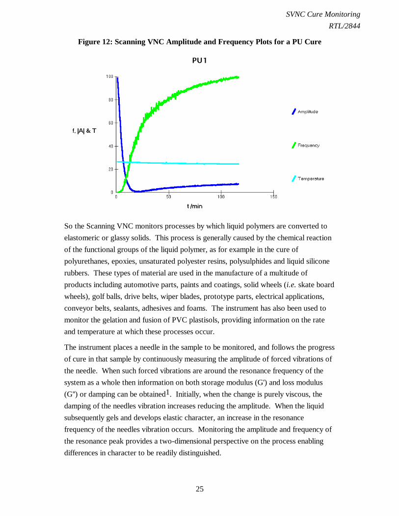
The Scanning VNC records the resonance amplitude and frequency, every 5 secondsor so (depending on computer speed) by recording the amplitude at three differentfrequencies. These points are fitted to a quadratic equation from which the maximum


24

amplitude and the resonance frequency are calculated. Figure 12 shows the amplitudeand frequency plots for a PU cure, the temperature of the sample holder is also shown.


25

Figure 12: Scanning VNC Amplitude and Frequency Plots for a PU Cure

So the Scanning VNC monitors processes by which liquid polymers are converted toelastomeric or glassy solids. This process is generally caused by the chemical reactionof the functional groups of the liquid polymer, as for example in the cure ofpolyurethanes, epoxies, unsaturated polyester resins, polysulphides and liquid siliconerubbers. These types of material are used in the manufacture of a multitude ofproducts including automotive parts, paints and coatings, solid wheels (i.e. skate boardwheels), golf balls, drive belts, wiper blades, prototype parts, electrical applications,conveyor belts, sealants, adhesives and foams. The instrument has also been used tomonitor the gelation and fusion of PVC plastisols, providing information on the rateand temperature at which these processes occur.

The instrument places a needle in the sample to be monitored, and follows the progressof cure in that sample by continuously measuring the amplitude of forced vibrations ofthe needle. When such forced vibrations are around the resonance frequency of thesystem as a whole then information on both storage modulus (G') and loss modulus(G'') or damping can be obtained1. Initially, when the change is purely viscous, thedamping of the needles vibration increases reducing the amplitude. When the liquidsubsequently gels and develops elastic character, an increase in the resonancefrequency of the needles vibration occurs. Monitoring the amplitude and frequency ofthe resonance peak provides a two-dimensional perspective on the process enablingdifferences in character to be readily distinguished.


26

The following examples show how the SVNC has been used to characterise the cure ofvarious types of resin.

3.1 Polyurethanes

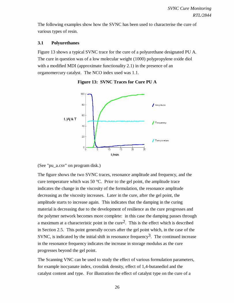
Figure 13 shows a typical SVNC trace for the cure of a polyurethane designated PU A.The cure in question was of a low molecular weight (1000) polypropylene oxide diolwith a modified MDI (approximate functionality 2.1) in the presence of anorganomercury catalyst. The NCO index used was 1.1.

Figure 13: SVNC Traces for Cure PU A

(See "pu_a.csv" on program disk.)

The figure shows the two SVNC traces, resonance amplitude and frequency, and thecure temperature which was 50 °C. Prior to the gel point, the amplitude traceindicates the change in the viscosity of the formulation, the resonance amplitudedecreasing as the viscosity increases. Later in the cure, after the gel point, theamplitude starts to increase again. This indicates that the damping in the curingmaterial is decreasing due to the development of resilience as the cure progresses andthe polymer network becomes more complete: in this case the damping passes througha maximum at a characteristic point in the cure2. This is the effect which is describedin Section 2.5. This point generally occurs after the gel point which, in the case of theSVNC, is indicated by the initial shift in resonance frequency3. The continued increasein the resonance frequency indicates the increase in storage modulus as the cureprogresses beyond the gel point.

The Scanning VNC can be used to study the effect of various formulation parameters,for example isocyanate index, crosslink density, effect of 1,4-butanediol and thecatalyst content and type. For illustration the effect of catalyst type on the cure of a


27

simple PU formulation is shown in Figures 14 and 15. PU A is that shown inFigure 13 and contains Thorcat 535 (0.53%) - an organomercury catalyst. PU B is thesame formulation except that the catalyst used is dibutyltin dilaurate (DBTL, 0.15%).

The traces clearly show significant differences between the two cure profiles. Themost obvious difference is in the final resonance frequency achieved, the formulationcontaining Thorcat 535 (PU A) reaching the higher resonance frequency (260 Hz forPU A and 150 Hz for PU B). The two formulations contain an excess of isocyanateand the Thorcat 535 catalyses the reaction of isocyanate with urethane groups(allophonate formation) more effectively than DBTL. Thus after 25 minutes theDBTL cure contains a higher proportion of unreacted isocyanate groups, reducing thestorage modulus of the material. In the Thorcat 535 cure these excess isocyanategroups become bound into the polymer network resulting in crosslinking and a higherstorage modulus. This difference in storage modulus (G'), which is related to hardness,is reflected by the difference in the final resonance frequency.

Figure 14: SVNC Frequency traces for Cures Containing Different Catalysts

(See "pu_a.csv" and "pu_b.csv" on program disk.)

The resonance amplitude trace responds to changes in the viscosity before gelation andin the loss modulus (G'') or damping after gelation. Thus the initial decrease in theresonance amplitude results from the increase in the viscosity of the formulation aschain extension progresses. These traces also reflect the progress of crosslinking inthese formulations (Figure 15). It has already been explained that the crosslink densityof the Thorcat 535 formulation increases more rapidly and how the resonancefrequency traces demonstrates this. The amplitude trace also shows this effect by theincrease in the amplitude during the later stages of the Thorcat 535 cure. This is dueto the reduction of the damping or loss modulus (G'') as the excess isocyanate groupsreact with the urethane groups.


28

Figure 15: SVNC Amplitude traces for Cures Containing Different Catalysts

(See "pu_a.csv" and "pu_b.csv" on program disk.)

3.2 Polysulphides

Liquid polysulphides are frequently used in sealants. Their proven ageing andweathering performance has found them wide use in the building industry whereas theirresistance to fuels has made them useful sealants for the fuel tanks of aeroplanes.

Figure 16 shows the Scanning VNC traces for the cure of a typical liquid polysulphidesealant. The curing agent used is manganese dioxide which oxidises the thiol endgroups of the polysulphide to disulphide linkages effecting chain extension andcrosslinking. As with the polyurethane example the increase in the viscosity in theearly stages of the cure is indicated by the decrease in the resonance amplitude. Thedevelopment of resilience, or reduction in damping, after the gel is indicated by theincrease in the amplitude during the later stages of the cure. The resonance frequency

Figure 16: SVNC Traces for the Cure of a Liquid Polysulphide

(See "sulphide.csv" on program disk.)


29

trace shows the increase in storage modulus or hardness as the cure progresses,reaching a final value of 170 Hz.

3.3 Silicones

Cured silicone polymers often have high resilience. The development of this resiliencecan be clearly observed using the SVNC as shown in Figure 17 which shows the cureof a silicone gum at 120 °C. Note the large increase in the resonance amplitude as theresonance frequency increases after the gel point.

Figure 17: SVNC Traces for the Cure of a Liquid Silicone

(See "silicone.csv" on program disk.)

3.4 Epoxy Cures

The examples described so far are for liquids that cure to rubbery solids. Generallyepoxides cure to hard and glassy plastics. This means that the cured products havevery high loss modulii which results in the resonance amplitude being very low. Thislimits the instruments ability to monitor to the very latest stages of this type of cure asit becomes increasingly difficult to locate the maximum of the resonance peak as theepoxide hardens causing the resonance amplitude to become very small (see SVNCOperating Manual RTL/2843 Sections 5.2 and 9). Ultimately the resonance peak maydisappear altogether.

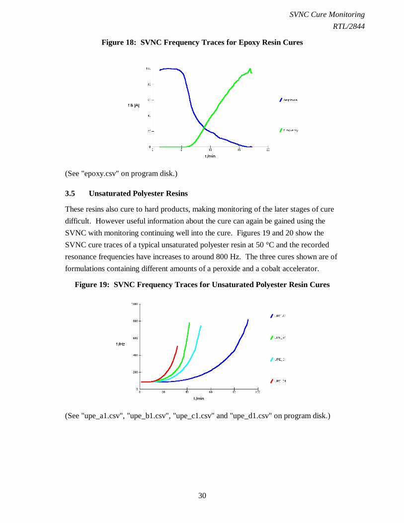
Although the instrument has this limitation for systems that cure to very hardproducts, it still provides useful information about these cures. Figures 18 shows theScanning VNC trace for a typical epoxy resin. The resonance frequency reached420 Hz before monitoring ceased.


30

Figure 18: SVNC Frequency Traces for Epoxy Resin Cures

(See "epoxy.csv" on program disk.)

3.5 Unsaturated Polyester Resins

These resins also cure to hard products, making monitoring of the later stages of curedifficult. However useful information about the cure can again be gained using theSVNC with monitoring continuing well into the cure. Figures 19 and 20 show theSVNC cure traces of a typical unsaturated polyester resin at 50 °C and the recordedresonance frequencies have increases to around 800 Hz. The three cures shown are offormulations containing different amounts of a peroxide and a cobalt accelerator.

Figure 19: SVNC Frequency Traces for Unsaturated Polyester Resin Cures

(See "upe_a1.csv", "upe_b1.csv", "upe_c1.csv" and "upe_d1.csv" on program disk.)


31

Figure 20: SVNC Amplitude Traces for Unsaturated Polyester Resin Cures

(See "upe_a1.csv", "upe_b1.csv", "upe_c1.csv" and "upe_d1.csv" on program disk.)

3.6 Visible Light Cure

With an appropriate initiator system vinyl or acrylic monomers can be cured by theaction of either UV or visible light. Figure 21 shows traces for duplicate cures oftriethyleneglycol dimethacrylate (TEGDMA) in the presence of a visible light initiatorsystem. The sample was place in a 4 mm deep sample holder and then the probe waslowered into it. Monitoring was started when a visible light (400 - 500 nm) was shone,via an optical guide, on the sample.

Figure 21: Fixed Frequency VNC Trace of Visible Light Initiated Cure ofTMPTMA.

(See "viscure1.csv" and "viscure2.csv" on program disk.)

3.7 PVC Plastisols

For the cure of thermosetting resins the amplitude and frequency responses are plottedagainst time, however the fusion of a PVC plastisol is a temperature dependant process


32

and the two sets of resonance data can be plotted against temperature. The SVNC canbe supplied with a temperature controller which allows the temperature of the heatstage to be increased in a controlled manner and by using a relatively thin film ofplastisol (e.g. 1 mm) the temperature of the liquid can be assumed to be that of theheat stage.

Figure 22 shows the percentage changes in the resonance amplitude and frequency asthe temperature is increased at 10 °C/minute. At temperatures up to about 80 °C thereis no change in the resonance frequency, indicating that the plastisol is still liquid.During this period the resonance amplitude increases slightly, reflecting the decrease inviscosity as the temperature of the liquid increases. At temperatures above 80 °C theresonance amplitude decreases, indicating that the viscosity is increasing, as thetemperature increases to 200 °C. The maximum rate of viscosity increase seems to beoccurring at about 125 °C. This increase in viscosity is caused by the plasticiserdiffusing into and swelling the particles of PVC.

Figure 22: Change in Resonance Amplitude and Frequency with IncreasingTemperature (10 °C/minute)

(See "pvc.csv" on program disk.)

The liquid does not become a solid (i.e. fusion) until the temperature reaches around120 °C. This is indicated by the temperature at which the resonance frequency firststarts to increase. After this point the plastisol cannot flow any longer. When thetemperature reaches 200 °C, the resonance frequency continues to increase, indicatingthat diffusion of the plasticiser into the particles occurs more slowly than thetemperature increase, thus when the temperature reaches 200 °C the diffusion processstill has some "catching up" to do for this particular plastisol.


33

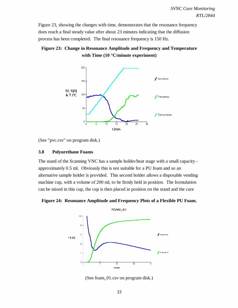
Figure 23, showing the changes with time, demonstrates that the resonance frequencydoes reach a final steady value after about 23 minutes indicating that the diffusionprocess has been completed. The final resonance frequency is 150 Hz.

Figure 23: Change in Resonance Amplitude and Frequency and Temperaturewith Time (10 °C/minute experiment)

(See "pvc.csv" on program disk.)

3.8 Polyurethane Foams

The stand of the Scanning VNC has a sample holder/heat stage with a small capacity -approximately 0.5 ml. Obviously this is not suitable for a PU foam and so analternative sample holder is provided. This second holder allows a disposable vendingmachine cup, with a volume of 200 ml, to be firmly held in position. The formulationcan be mixed in this cup, the cup is then placed in position on the stand and the cure

Figure 24: Resonance Amplitude and Frequency Plots of a Flexible PU Foam.

(See foam_01.csv on program disk.)


34

monitored (see SVNC Operating Manual RTL/2843 Section 7.2). In this test about30 g of material was mixed in a suitable cup and the cure monitored.

Figure 24 shows a Scanning VNC trace for a flexible foam, comparing the resonancefrequency, indicative of changes in the elasticity or modulus of the sample, andresonance amplitude, indicative of changes in the viscosity of the sample.

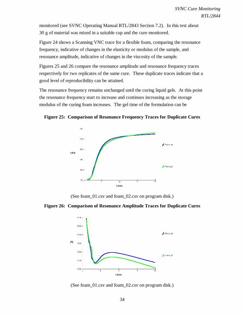
Figures 25 and 26 compare the resonance amplitude and resonance frequency tracesrespectively for two replicates of the same cure. These duplicate traces indicate that agood level of reproducibility can be attained.

The resonance frequency remains unchanged until the curing liquid gels. At this pointthe resonance frequency start to increase and continues increasing as the storagemodulus of the curing foam increases. The gel time of the formulation can be

Figure 25: Comparison of Resonance Frequency Traces for Duplicate Cures

(See foam_01.csv and foam_02.csv on program disk.)

Figure 26: Comparison of Resonance Amplitude Traces for Duplicate Cures



35

estimated by calculating the time at which the frequency trace has increases by 5% ofits total change. In the case of the two traces of Figure 25 this occurs after 2.3 and2.1 minutes. Formulation changes, for example isocyanate index, may be expected toaffect the final modulus of the cured foam and this would be reflected in differing finalresonance frequencies.

The amplitude traces (Figure 26) show the changes in the damping character of thecuring formulation. The initial decrease in resonance amplitude is caused by theincrease in viscosity that occurs before the gel point. In these traces a minimum occursjust after the gel point at 3.8 and 3.6 minutes. This minimum indicates the point ofmaximum damping and the subsequent increase in resonance amplitude is the result ofan increase in the resilience of the foam as the crosslink density continues to increase.The decrease in amplitude that occurs after about 8 minutes is most probably due tothe effect of the foam cooling as the exotherm subsides.

The SVNC is also capable of monitoring temperature, for example via a thermocoupleplaced in the curing sample.

The Scanning VNC can also be used to monitor the cure of rigid foams. Figures 28 to30 show traces for such cures.

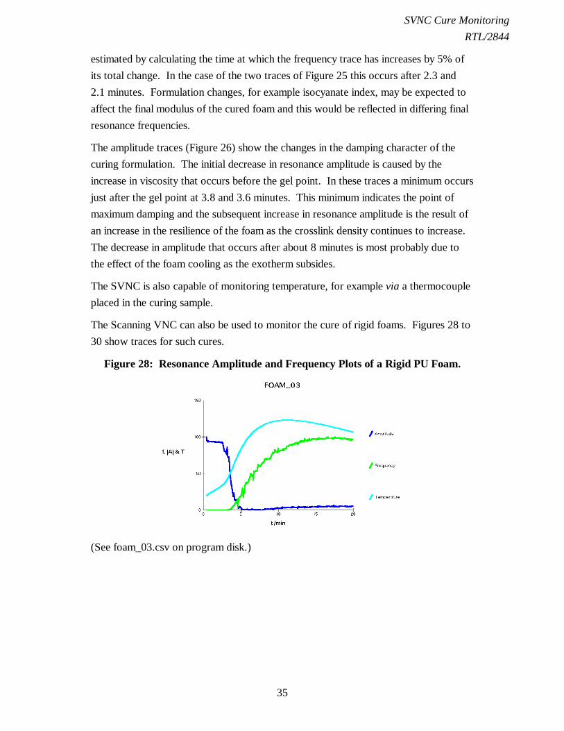
Figure 28: Resonance Amplitude and Frequency Plots of a Rigid PU Foam.

(See foam_03.csv on program disk.)


36

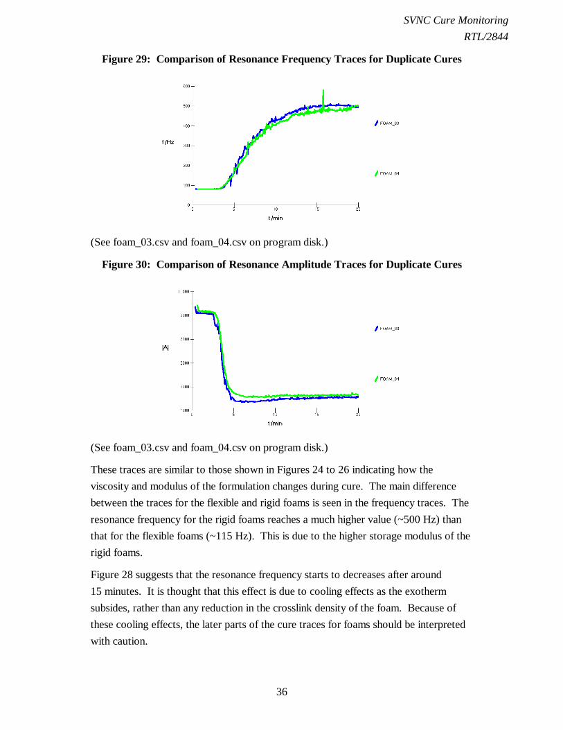
Figure 29: Comparison of Resonance Frequency Traces for Duplicate Cures


Figure 30: Comparison of Resonance Amplitude Traces for Duplicate Cures


These traces are similar to those shown in Figures 24 to 26 indicating how theviscosity and modulus of the formulation changes during cure. The main differencebetween the traces for the flexible and rigid foams is seen in the frequency traces. Theresonance frequency for the rigid foams reaches a much higher value (~500 Hz) thanthat for the flexible foams (~115 Hz). This is due to the higher storage modulus of therigid foams.

Figure 28 suggests that the resonance frequency starts to decreases after around15 minutes. It is thought that this effect is due to cooling effects as the exothermsubsides, rather than any reduction in the crosslink density of the foam. Because ofthese cooling effects, the later parts of the cure traces for foams should be interpretedwith caution.


37

In general foaming formulations have to be designed so that the rise occurs before thegel time. Thus as the formulation is foaming it is still a viscous liquid and so is able torise around the instruments probe/needle. Obviously there are many process occurringduring the cure of a foam, changes in viscosity, temperature, density and depth ofneedle/probe penetration. The traces obtained are the result of a combination of theseeffects, albeit the traces can be used as a useful measure of the process of cure duringthe formation of a PU foam. The instrument does not give any indication of the foam'srise, however the data obtained can be used in conjunction with such data to provide acomprehensive characterisation of the foaming process.

The cure of the rigid foam shown in Figures 29 and 30 is fairly slow. Figures 31 and32 show the SVNC traces for a typical refrigerator insulation PU foam which has asignificantly faster cure. These cures were monitored using the Fast Cure option of theSVNC menu rather than the Monitor option.

Figure 31: Resonance Frequency Traces for a Typical Insulation PU Foam


Figure 32: Resonance Amplitude Traces for a Typical Insulation PU Foam


38


3.9 Cure Monitoring of Thin Films

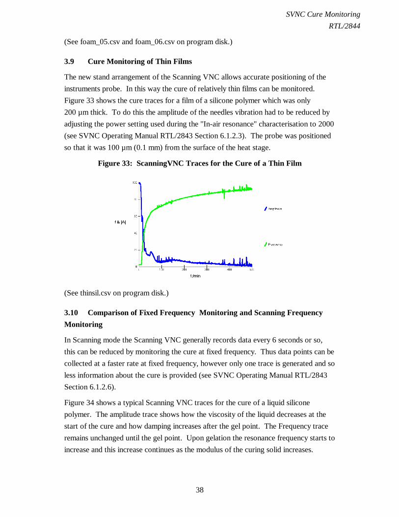
The new stand arrangement of the Scanning VNC allows accurate positioning of theinstruments probe. In this way the cure of relatively thin films can be monitored.Figure 33 shows the cure traces for a film of a silicone polymer which was only200 µm thick. To do this the amplitude of the needles vibration had to be reduced byadjusting the power setting used during the "In-air resonance" characterisation to 2000(see SVNC Operating Manual RTL/2843 Section 6.1.2.3). The probe was positionedso that it was 100 µm (0.1 mm) from the surface of the heat stage.

Figure 33: ScanningVNC Traces for the Cure of a Thin Film

(See thinsil.csv on program disk.)

3.10 Comparison of Fixed Frequency Monitoring and Scanning FrequencyMonitoring

In Scanning mode the Scanning VNC generally records data every 6 seconds or so,this can be reduced by monitoring the cure at fixed frequency. Thus data points can becollected at a faster rate at fixed frequency, however only one trace is generated and soless information about the cure is provided (see SVNC Operating Manual RTL/2843Section 6.1.2.6).

Figure 34 shows a typical Scanning VNC traces for the cure of a liquid siliconepolymer. The amplitude trace shows how the viscosity of the liquid decreases at thestart of the cure and how damping increases after the gel point. The Frequency traceremains unchanged until the gel point. Upon gelation the resonance frequency starts toincrease and this increase continues as the modulus of the curing solid increases.


39

It can be seen that both the resonance frequency and resonance amplitude are stillchanging after 100 minutes of cure, indicating that the cure process is incomplete atthis stage.

Figure 34: Scanning VNC Trace for a Liquid Silicone Polymer

(See sil_scan.csv on program disk.)

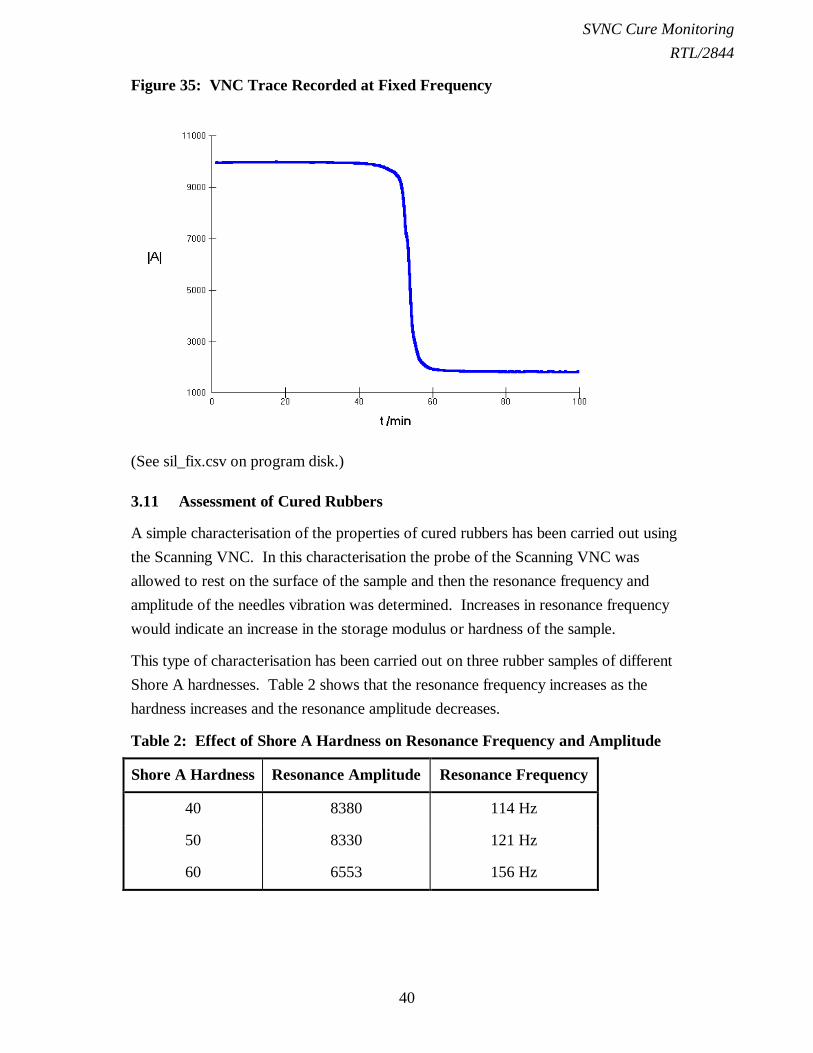
Figure 35 shows the single trace monitored at fixed frequency for the cure of the sameformulation. This trace is affected by both changes in viscosity and modulus. In theearly part the trace is predominantly representative of changes in the viscosity of thesample. The later part of the trace is mainly affected by the modulus of the curingsolid. Thus a single trace is produced which is representative of the cure, however it ismore difficult to interpret this simple trace in terms of viscosity and modulus changesthan the dual trace of the Scanning VNC. However there is the potential for recordingdata more quickly with the fixed frequency option. Figure 35 shows that the tracestops changing after about 70 minutes, however the trace of Figure 34 shows thatchanges are still occurring after 100 minutes. Thus in the fixed frequency mode theinstrument cannot detect the changes occurring during the later stages of the cure.


40

Figure 35: VNC Trace Recorded at Fixed Frequency

(See sil_fix.csv on program disk.)

3.11 Assessment of Cured Rubbers

A simple characterisation of the properties of cured rubbers has been carried out usingthe Scanning VNC. In this characterisation the probe of the Scanning VNC wasallowed to rest on the surface of the sample and then the resonance frequency andamplitude of the needles vibration was determined. Increases in resonance frequencywould indicate an increase in the storage modulus or hardness of the sample.

This type of characterisation has been carried out on three rubber samples of differentShore A hardnesses. Table 2 shows that the resonance frequency increases as thehardness increases and the resonance amplitude decreases.

Table 2: Effect of Shore A Hardness on Resonance Frequency and Amplitude

Shore A Hardness Resonance Amplitude Resonance Frequency

40 8380 114 Hz

50 8330 121 Hz

60 6553 156 Hz


41

3.12 Summary

The SVNC is a simple, robust instrument which is capable of recording the progress ofthe cure of liquids and pastes setting to rubbers or glasses. This relatively low costcuremeter is designed for use by non-rheologists, however it is capable ofdistinguishing the effect of various formulations changes. This is achieved by separatelycharacterising cure in terms of the viscous and elastic changes providing informationon key cure parameters: onset of viscosity increase; gel time; build up of modulus andresilience. This Section has illustrated this ability with respect to PU, polysulphide,silicone, epoxy and unsaturated polyester cures as well as the fusion of a PVCplastisol. The SVNC is ideal for both development of new formulations and qualitycontrol during production.

3.13 References

1. R.W. Whorlow, "Rheological Techniques", Ellis Horwood, Chichester, 1989,pp270-272.

2. C.W. Macosko, "Rheological Changes During Crosslinking", Br. Polym. J.,1985, 17, 239-245

3. B.G. Willoughby, K.W. Scott and D. Hands, "Cure Rationalisation Using aVibrating Needle Curemeter", Rapra Seminar "Flow and Cure of Polymers -Measurement and Control", Shawbury, 22-23 March 1990.


42

INDEX

AApplication Time, 3BBranching Theory, 3CChain Extension, 3, 31Complex Viscosity, 8Computer, 16Crosslink Density, 11, 15Crosslinking, 3, 31Cure, 1, 3, 15, 31

Application Time, 1, 3Branching Theory, 3Chain Extension, 3, 31Changes During, 15Complete, 4Crosslinking, 3, 15, 31Damping, 32Demould, 1Elasticity, 3, 15

Entanglements, 15Epoxy, 36Exotherm, 16Gel Point, 1, 3, 5, 11, 15Gel Time, 14, 26Glassy, 1Glassy Products, 36, 37Hard Products, 36, 37Liquid Polymer, 3Model System, 11Modulus, 3Molecular Weight, 4Monitoring, 19Network, 3Network Flaws, 15Onset of, 4Polysulphide, 35Polyurethane, 32

Foam, 40Flexible, 41Rigid, 42

Profile, 1Resilience, 31, 36

Sealant, 35Silicone, 36State of, 4Thin Films, 45Unsaturated Polyester Resin, 37Viscosity, 15Viscous, 32Visible Light, 38Vitrification, 1Work Life, 1, 3, 15

DDamping, 1, 8, 11

Maximum, 11EElasticity, 1, 3, 15Entanglements, 15Epoxy, 36Exotherm, 16FFixed Frequency, 45Fluid Flow, 4Frequency, 26GG', 15G'', 15Gaussian condition, 3Gel Point, 3, 5, 11, 15, 30, 32Gel Time, 14, 26LLiquid Polymer; Cure, 3Loss Modulus, 8, 11MMaximum Damping, 11Modulus, 3

G', 9, 15, 32G'', 9, 15, 32In-phase, 7Loss, 8, 11Out-of-phase, 7Stiffness, 3

Molecular Weight, 4Monitoring, 3, 31

Amplitude, 32


43

Fixed Frequency, 45Frequency, 32

Elasticity, 30Monsanto Rheometer, 7Oscillatory Measurements, 5PVC Plastisols, 38Resilience, 31Resonance, 19

Amplitude, 19Frequency, 19

Resonance Peak, 31Rheometers, 15Thin Films, 45Two-dimensional, 31, 32Visible Light Cure, 38

Monsanto Rheometer, 7NNetwork, 11

Formation, 14Network Flaws, 15OOscillatory Measurements, 5PPhase Angle, 7, 8Polysulphide, 35Polyurethane, 33

Foam, 40Flexible, 41Rigid, 42

Gel Point, 33Resilience, 33Storage Modulus, 33Trace, 34, 35

Process Control, 3Product Control, 3PVC Plastisols, 38RResilience, 31Resonance

Amplitude, 19Frequency, 19

Resonance Frequency, 26Rheometers, 15SScanning VNC, 15, 16Sealant, 35

Polysulphide, 35

Shear Modulus, 4Silicone, 36State of Cure, 4Stiffness, 3Storage Modulus, 8TThin Films, 45Trace

Damping, 1Elastic, 1

Transducer, 16, 19, 23Model, 19, 23

Elastic, 27UUnsaturated Polyester Resin, 37VVibrator, 16, 19, 23

Elastic Model, 27Model, 19, 23

Visco-elastic, 7Viscosity, 4, 15, 24

Amplitude Attenuation, 24Complex, 8

Viscous Properties, 3WWork Life, 3, 15

cure information svnc

Documents