cultural and biological evolutionary processes, selection...

THEORETICALPOPULATIONBIOLOGY~, 238-259(1976)

Cultural and Biological Evolutionary Processes, Selection for a Trait under Complex Transmission*

MARCUS W. FELDMAN

Department of Biological Sciences, Stanford University, Stanford, California 94305

AND

L. L. CAVALLI-SFORZA

Department of Genetics, Stanford University School of Medicine, Stanford, California 94305

Received June 1, 1975

We consider the evolution of a trait, which is under both genetic and phenotypic transmission. An individual is always born in one state but can be converted to the other before reaching adulthood. If the conversion takes place by a learning process, the native state is called “unskilled,” and that acquired by learning is called “skilled. ” If phenotypic conversion takes place by way of infection, the native state is uninfected, and can be converted to infected. Native and converted phenotypes may be subject to selection; acquiring a skill may lead to selective advantage of skilled versus unskilled, while contracting a disease may involve a selective disadvantage. Conversion probability is a function of the parental phenotypes. In some of our models we assume that only one parent has teaching ability (or transmits the disease) and in others we consider more general situations. The probability of learning (or of taking the disease) may be determined by the individual’s genotype. A diallelic locus is considered. The evolution of the genotypes and the phenotypes is studied in a variety of situations. Equilibria, and in a few simple cases the dynamics of the phenotypes and genotypes in the population are given. The usual equilibrium for heterozygote advantage is found to depend, in the present case, on the parameters of the learning process. Oscillatory equilibria and more than one stable equilibrium can exist in certain circumstances. Even in the absence of genotypic differences for the conversion probability gene frequencies may change.

1. INTRODUCTION

The quantitative theory of genetic change in populations is one of the most highly developed subdisciplines of theoretical biology. This is especially true for single gene loci, or small numbers of loci with well-defined effects. The

* Research supported in part by NIH Grants USPHS 10452-10-11, 20467-02, NSF Grant GB 37835 and USAEC AT(04-3)-326.

238 Copyright 0 1976 by Academic Press, Inc. AU rights of reproduction in any form reserved.

CULTURAL AND BIOLOGICAL PROCESSES 239

dynamics of the change of characters that are not controlled in a simple genetic way but that depend on interactions with the environment is one of the under- developed areas of population genetics. We have been especially interested in the transmission and evolution of cultural traits that are influenced by the familial environment, and by the group into which an offspring is born (Cavalli-Sforza and Feldman 1973a, b, Feldman and Cavalli-Sforza, 1975). In one of these studies we addressed the question of the interation between genotype and phenotype by assuming that a child’s phenotype was linearly regressed on the midparental phenotype, but in such a way that the regression coefficient depended on the child’s genotype. There are obvious generalizations to the case where the regression coefficient depends on both parental genotypes as well.

The simple model was amenable to some analytic treatment. A central objective of that study was to track changes in population statistics, such as parent-offspring and sib-sib correlations, as well as heritability, over time. (A completely different approach to the same subject was taken by Morton (1974) and Rao, Morton, and Yee (1974). The graphical analysis by Lewontin (1974) however, is similar in many respects to our formulation.) In these studies we considered the gene frequency to be fixed, and we assumed random mating and no natural selection. Some of these restrictions have been lifted in a study by D. Wagener (in preparation).

Most studies of the dynamics of phenotypes have concentrated on the statistics of the continuous traits. Kimura (1965) analysed a one locus model with mutation and stabilizing selection. He used a quadratic deviations fitness function and allowed mutation to cause small changes in allelic effects. He showed that under these assumptions the equilibrium distribution of allelic effects was approximately normal. Latter (1970), used a different approach to obtain a formula for the amount of genetic variance that could be maintained. The analysis by Slatkin (1970) was restricted to properties of the equilibrium phenotypic variance in a “polygenic” model and was not concerned with any equilibrium properties of such genotypic variables as gene or chromosome frequencies or the genetic contribution to the phenotypic variance. Lande’s recent studies of more general models of the Slatkin type does address the issue of heritability, but without reference to allele frequencies at specific loci (Lande, 1975).

In the present paper we study models in which the probability of transmission of a discontinuous phenotype to an offspring depends only, or largely, on whether one or both of its parents had the trait. Individuals are classified into those who have the trait, called skilled, and those who do not, called unskilled. It is our purpose to study situations in which the acquisition of the skill may carry with it a selective advantage (or disadvantage). We consider a single diallelic locus which may affect the presence or absence of the skill.

240 FELDMAN AND CAVALLI-SFORZA

“Skilled” and “unskilled” are the only possible phenotypes. We first develop a more general form of the model which allows learning differences among the genotypes, and genotypically determined selection values for the trait. In most of the models presented here we assume that only one parent is involved in the transmission of the trait. Biparental extensions are obvious, and an example is contained in Section 7. However, in the more general model and in most special cases the assumption of uniparental teaching is retained.

We demonstrated (Cavalli-Sforza and Feldman, 197313) previously that the dynamics of change in statistics for a phenotype in a population may be strongly affected by interactions between the parent’s and the offspring’s phenotypes and genotypes. One of our main purposes here is to demonstrate how selection on a culturally determined character can cause changes in gene frequency. We shall also show how, under special circumstances, gene frequencies can change even if there are no genetic differences in learning ability.

We commence with the structuring of a general uniparental model. In subsequent sections we discuss a number of special simpler cases in which there are no genotypic differences in selection and in some of which there are special assumptions about the mode of transmission of the skill.

2. A GENERAL UNIPARENTAL TRANSMISSION AND SELECTION SCHEME

Consider a simple diallelic genetic locus at which the frequencies of alleles A and a are p and p, respectively. In addition to their genotype, individuals are characterized by the phenotype of having or not having a certain unspecified skill. Within the genotypes AA, Aa, aa the skilled individuals are denoted --- AA, Au, aa, and the unskilled ones AA, Au, aa. The proportions of the respective genotypes that are skilled are K, , k, , k, at a given generation. Thus, K, is the number of AA divided by the combined number of AA and AA, etc. Mating occurs at random with respect to skill and genotype. One parent, who may or may not be skilled, is arbitrarily defined as the teaching parent. If the teaching parent is skilled the probabilities that the offspring of genotypes AA, Aa, and aa are unskilled are respectively Ni , iVa , and Na . If the teaching parent is unskilled they are n, , n2 , 11s . Finally we suppose that selection occurs and that it depends on the acquisition of the skill. The relative survival rates of __- AA, Au, iii, AA, Au, au are 1 + sr , 1 + sa , 1 + s, , 1 + t, , 1 -t t, , 1 f t, , respectively.

To track the changes in the various frequencies from one generation to the next we introduce the genotype frequencies u, v, and w of AA, Aa, and aa, respectively. All 36 possible matings, their frequencies and the probabilities of the various classes of offspring may then be tabulated. The list is recorded as Table I.


It is easy to see, by adding the appropriate groups of frequencies that after the first generation the genotype frequencies AA, Au, and au are in fact the products of the respective gene frequencies. Therefore, we may reduce the consideration of the variables u, V, and w to that of p, the frequency of A in the population. Again, by adding the appropriate offspring frequencies of -- AA, Aa, and Zi, and dividing by the new genotype frequencies, we obtain a recursion system for k, , k, , and k, in terms of these variables, and the gene frequency in the previous generation. The complete four-dimensional recursion system is presented as equations (I), (2) (3), and (4) with Q = 1 - p.

p[l _L WI + h(l PI = 1 + (Slk, + tl( 1 - K,)} pa

- u P + bk, + a - WI1 + 2{s,k, + t,(l - k,)) pq +{& + &(I - &,F ’ (l)

k,’ =

(I--n,)[p(l-k,)(l+t,) + q(l--k,)(l +f,)l + (~--NJW~~+SI) + @2(1+s2)1

1 +p[& + tl(l - k,)l + ds2k2 + t2U - k2)l (4

k 2 , = ~(l-n,)[p(l-k,)(l +~,>+q(1-k,)(~+~,)l+(l-~,)[pk,(l+s,)+qk,(l+sz)l 2 - 1 + p[& + tl(l - k,)l + d& + t2U - kJ1 I (I-n2)[p(l-k,)(1+~,)+q(l-~,)(1+~,)l+(l-~,)C~~~(l+~,)+qk,(~+s~)l i-

’ 2 1 + p[& + te(l - &)I + q[& + t&l - &)I (3)

k , =(l-n3)[p(l-k2)(1+t2)+~(1--3)(1+t3)1+(1-~3)IPk2(1+s~)+qk3(l+s,)l 3 1 + p[s,k, + tz(l - &)I i- q[& + h(l - kdl

(4) The full four-dimensional system, which involves 12 parameters (actually 11 since we can normalize the viabilities), is clearly very complicated. It is easy to see that apart from states of genetic fixation ( p = 0, p = 1) any isolated equilibrium of the system must satisfy

j?Jz {S3R3 + ta(1 - R,)) - {stfip + t20 - R2)

Sff (5)

1 1 + t1( 1 - Al) f S3R3 + i3( 1 - R,) - 262ff2 + f2(1 -m ’

where the circumflex denotes equilibrium values of the variables, provided the right side of (5) is meaningful.

For (5) to be admissible (i.e., 0 < j < 1) we require restrictions on A, ,

A2 7 and A, . But these equilibrium values are difficult to extract from the system of three simultaneous cubic equilibrium equations. For this reason we have chosen a set of less general parametrizations for which equilibrium theory, and in some cases time dependent theory, can be obtained. In all of the analysis that follows we set si = sa = sa = s and t, = t, = t3 = 0. Thus, the relative viability of a skilled to an unskilled phenotype is 1 + s : 1. This is a substantial simplification, but does cover the important case where selection is completely

TABL

E I

Mat

ing

Tabl

e fo

r Le

arne

d Sk

ill”

hl

R

Teac

hing

O

ther

pare

nt

x pa

rent

-~__

-.--

AA

x AA

- AA

x

AA

AA

x AA

AA

x AA

AA

x Aa

%i

x Aa

AA

x Aa

AA

x Aa

- AA

x

z.i

- AA

x au

AA

x z

AA

x au

A,

x AA

A<

x AA

Aa

x AA

Aa

x AA

Prob

abilit

y of

offs

prin

g

Freq

uenc

y of

mat

ing

(AA)

(A

Al

(Aa)

k,(l

- k&

l +

sd(l

+ t,W

/T2

k,(l

- k,

)(l

-I s&

l +

t&2/

T”

(1 -

k,

)2(1

+

t,)W

/F

k,k,

(l i-

SIN

+

S&J/

T2

kl(l

- k,

)(l

+ s&

l +

thvl

T*

Ml

- k&

l i

sz)(l

+

t&m

/T*

(1 -

k&

l -

k,)(l

+

tJ(l

+ t&

W

f&(1

3

sd(l

+ s,

W/T

2

k,(l

- k,

)(l

+ sI

)(l

$- t

&u/

T2

Ml

- M

l -t

s:dl

+

t&w

/P

(1 -

k,

)(l

- M

l +

Ml

+ t,W

IT*

k&,(1

+

s&l

+ s,

)u~/

T2

Ml

- k&

l i-

d(l

+ tJ

w/T

2

k,(l

- k,

)(l

+ sA

(l i-

t&o/

T2

(1 -

k,

)( 1

-. k&

l -i-

tJ(

l +

t&u/

T*

NJ2

N

J2

n,P

42

1 -

Nl

1 -

NI

I -

?lt

1 -

111

(1 -

N

J/2

NJ2

(1

-

NM

. N

J2

(1 -

41

2 %

I2

(1 -

d/

2 42

N

2

N2

%

n,

(1 -

N

,)P

NJ2

(1

-

Nd/

2 N

J2

(1 -

d/

2 %

I2

(1 -

d/

2 %

I2

(1 -

N

dl2

(1 -

N

N

(1 -

f-d

/2

(1 -

74

12

1 -

Nr

1 -

N2

t-112

1 -

n2

(1 -

N

AP

.

(1 -

N

J2

(1 -

flz

)P

(1 -

%

)P

AU

Z A a

A a

Aa

- Aa

Aa

Aa

aa

aa

aa

all

zi

z aa

aa

zi

aa

aa

na

X Z

X Aa

X Z

X AU

X aa

X aa

X an

X aa

X AA

X AA

X AA

x AA

-

x Aa

X Aa

X A<

X Aa

X ;i;

;

X aa

x aa

X aa

k,(l

- k,

)(l

i- SP

)(l -

IF L

w/T

2

k,(l

- k,

)(l

-I- s

z)(l

+ hW

/T’

(1 -

k,

)“(l

-I- t

2)‘u

2/T”

k,k,

(l i-

s,)(l

+-

s&w

/T’

k,(l

- k&

l +

s&l

+ @

J~/~

”

k,(l

- k&

l +

~a)(1

+

G.)‘

Jw/T

~

(1 -

k?

)(l

- k&

l -b

b)(l

-1

b)~

w/T

’

kIk,

(l -I-

s,)(

l +

c,)u

w/T

2

k,(l

- k,

)(l

i- s&

l +

hh/~

*

kl(l

- k,

)(l

-t sz

)(l

+ ts

)w~/

~’

(1 -

k&

l -

k&l

+ h)

(l -I’

- t&

u/T”

k,k,

(l f

s,)(l

+

s,)w

/T*

k,(l

- k&

l +

c,)(l

+

@-‘w

/~”

k&l

- k&

l +

s&l

+ t&

w/T

”

(1 -

k,

)(l

- k&

l -t

t&l

i- C

&w/T

”

ka2(

l +

s@u2

/T”

k,(l

- k,

)(l

-I- s

,)(l

+ h)

w’/~

’

k,(l

- k,

)(l

+ %

)(l

+ hh

2/T2

(1 -

k,

)yl

+ t&

uZ/T

2

NJ4

(1

-

N1)

/4

N2/

2 N

J4

(I -.-

N,)/

4 N

zP

9111

4 (1

.-

d/4

742

%I4

(1

-

d/4

42

NJ2

N

J2

%I2

“2

P

NZ

N2

n2

n2

NJ2

N

J2

4 %I2

(1 -

N

&2

N,/4

(1 -

N

&/2

N,/4

(I --

n,)/2

nJ

4

(1 -

%

)/2

%/4

(1 -

N

,)/2

NJ2

(1 -

N

J/2

Nd

(1 -

d/

2 4

(1 -

74

12

&,I2

1 -

Nz

1 -

N2

1 -

n2

1 -

n,

(I -

NdP

N

,/2

(1 -

N

W

NJ2

(I

- d/

2 42

(1 -

d/

2 d2

N3

N:,

,23

123

(1 -

N

,)/4

(1 -

N

J/4

(1 -

%

)/4

( 1 -

%

)/4

(1 -

~ N

J2

(1 -

N

3)/2

(1

-

d/2

(1 -

%

)/2

(1 -

N

3)/2

(1 -

N

dD

(I -

nm

(1 -

%

)P

1 -

N3

1 -

N,

1 -

ng

1 -

Tl3

u T

is a

nor

mal

izin

g fu

nctio

n,

T =

tr[k,

(l +

sz)

+ (1

-

MI

+ h)

l -t

v[k,

(l -i-

~2)

+

(1 -

k,

)(l

+ &)

I -t

w[k

,(l

+ 3s

) -F

(1

- k,

)(l

-t &,

)I.


phenotypic. The various models that follow involve assumption on the transmission parameters Ni and ni . We shall refer to the general model (l)-(4) as model G.

3. SOME RESULTS FOR THE GENERAL MODEL WITH SELECTION FOR SKILL ONLY (MODEL SS)

Set si = s, ti = 0, (; = 1, 2, 3) in (l)-(4). The system is now one with essentially seven parameters. Writing CL( = 1 - ni and /3i = (1 + s)( 1 - Ni) - 01~) (; = 1, 2, 3) the system (l)-(4) is more simply expressed as

P’ = p(1 + sW(l + SK), (6) kl’ = (a1 + fvG)/U + SK), (7)

k,’ = ww% + B,w(l + SK,) i 6% + 13,fGMl + &)I~ (8)

4 = (aa + &~2)/(1 + sm (9)

where K1 = pk, + qk, , K2 = pk, + qk, . The K1 and K, are in some sense marginal effects of the skill. K = pK, + qK, is the mean skill in the population. Rewriting (6) as

P’ = P + sPq(K, - &Ml + SK), (6’)

it is easy to see that the equilibria for p are of the form $ = 0, j = 1, and, from KI = K, ,

b = (6 - Q/(4 + A, - 2&h (10)

where the hats denote values at equilibrium. If $ = 0, then from (9), if 01~ + 0, a single valid equilibrium value of k3 is obtained as the root of a quadratic equation. We call this k, . ^(‘) When substituted into (8), this produces a single valid value &Lo) as the root of a quadratic equation. Together &” and xi” produce a unique &“‘. We denote this solution ($ = 0, ii’), &‘), &“) by S(O). Similarly there is an equilibrium ($ = 1, &:I’, &I, @)), which we denote by S(l).

It is not difficult to see that L?(O) is stable when s > 0 only if A$‘) > xi’), or when s < 0 only if &‘) < xi’). Note here that if 01~ (or 01~) is zero then so is &, (or L,). From these boundary facts we infer that a gene frequency polymorphism at equilibrium entails that, if it is advantageous, the skill is more frequent at equilibrium among the heterozygotes than the homozygotes. This says nothing about the form of the polymorphism, although (10) . IS o b viously a candidate. We shall see that the full picture is more complicated than this.

The (genetic) polymorphic equilibrium (10) is explicitly determined from (7)-(9) with Kip) = K.$“‘. Th e superscriptp denotes the polymorphic equilibrium, which henceforth will be called S(p). In fact we must have


where K(p) solves the cubic equation

k’3wl + 83 - %)I

+ WPl + P3 - 282 + 4% + a3 - 2012) - w3 - A”)1 + K[ol, + 013 - 2% - 433 - 0[3/31 + 2&J + %2 - %%7 = 0 (11)

It is therefore conceivable that three polymorphic solutions exist for the average frequency of skill in the population. Rather than work with the full seven parameter system, we have assumed in most of what follows that CQ = 0 for all i. (That is, an unskilled teaching parent does not produce skilled offspring.) It may be that this assumption alters some of our qualitative conclusions. However, in some of the subsequent sections we relax this assumption (while making others) so that certain speculations concerning the more general case can be made.

4. EQUILIBRIUM ANALYSIS OF MODEL SS WITH oli = 0

As in the general case, at equilibrium we must have j = 0 or $ = 1 or &i = K2 . The case $ = 0 is analogous to the solution So) in the case where ai # 0. But with oli = 0 (all ;) there are three possible solutions with j = 0. They are

$ = 0; /$, = A2 = A, = 0 (124

$ = 0; $1 = 032P - lM32/2& 9 & = @,/2 - 1)/s, L, = 0 (12b)

$ = 0; A, = /&r”/(l + S@), 4s = YO, L, = (p3 - 1)/s, W)

where r” is the valid root of

Sk2 + kz[ 1 - /32/2 - &A3/2( 1 + d3)] - &r;,/Z( 1 + si3) = 0.

A set corresponding to (12a)-(12c) with j = 1 clearly also must be considered; of interest to us is the point

1; = 1; 6, = (fil - 1)/s, L, = Yl, L, = j33Yi/(l + Vi), (124

where r1 is the valid root of

sk22 + k,[l - /3,/Z - $2&/2(l + sff,)] - /3,&/2(1 + &) = 0.

Note that (12b), (12c), and (12d) are admissible only if s > 0. Further, (12~) requires is, > 1, (12d) requires fir > 1, and (12b) requires p2 > 2.


Remark 4.1. When CQ # 0 for all i, (12a, b, c) reduce to a single equilibrium. With s > 0 and 01~ small (necessarily positive) this equilibrium, S(O), is close to (12~). With s < 0 and 01~ small S(O) . 1s close to (12a). Similar considerations apply to S’(l) when cli are small, with reference to (12d).

Equilibrium (12b) can never be stable, while (12a) always has a unit eigenvalue. On the other hand (12~) is locally stable if and only if & > A, (since its existence entails s > 0). This in turn reduces to the elegant condition /?a > pz . Similarly, if 81 > fiz the analogous $ = 1 equilibrium is locally stable. Thus, if skill is selected for (s > 0) and the selection is strong enough (pB > 1, p1 > 1) so that (12~) and (12d) exist, then we expect genetic polymorphism to be maintained if the heterozygotes are more receptive to the skill of their parents than are the homoxygotes.

Remark 4.2. From (7)-(9) it is clear that even though (12a) has a unit eigenvalue, it cannot be stable while (12b) and (12~) exist. If (12a) is stable, it has an eigenvalue of unity and neither (12b) nor (12~) exist.

Remark 4.3. In this situation LY~ = 0 for all i, an interesting new special class of equilibria exists in addition to S to), S(l), and S(P). If A1 = x, = L, = 0, then the system is in equilibrium for any p value. This neutral one parameter family of equilibria is denoted ,!P).

S(n) = {p, R, = 0, A, = 0, x, = 0). (13)

To elucidate the interaction of selection and differential transmission of the selected character as an evolutionary force, it is necessary to study the stability properties of the equilibria S(O), S(l), S(*), and Stn) in some detail.

We have already remarked that the (gene frequency) boundary equilibrium (12~) exists when s > 0, & > 1 and is stable if & > f12 . Solution (12d) exists when s > 0, is, > 1 and is stable if ,Q1 > pz . If s < 0, neither (12b) nor (12~) exist. When ai = 0 we return to (11) and see that either R = 0 or

R(“) = (A83 - 82”) - (A + 163 - 332) = @d = @de

@l + 83 - 332) (14)

The solution & = 0 is Sn) as defined in (13). The polymorphic isolated equilibrium (14) has

P ̂fp) = (A - P2Wl + A - 2@2), (15)

and clearly requires either & > pz , p3 > p2 , or & < & , &, < fi2 for existence. It is straightforward to show that if s < 0 this polymorphic solution (14), (15) cannot exist since the constraint 0 < R (p) ,( 1 is violated. In other words, if the skill is selectively disadvantageous and if offspring attain the skill only by transmission from a skilledparent, no isolatedpolymorphicgene frequency equilibrium


can be attained. When s > 0, from (14) the admissibility condition 0 < R(P) < 1

reduces to

w% - 822M81 + A - 332) > 1) (16)

irrespective of whether /Ii , /3s > f12; or /I1 , & < P2 . From (14), (IS), and (6), (g), and (9) at equilibrium, &‘), xi”), and &AP) may be found. A linear analysis in the neighborhood of this equilibrium reveals that it is locally stable provided

(a) (16) holds, and (b) A < I% , A < PZ - Closer scrutiny of these stability conditions provides further information

on the interaction between differential receptivity to the skill and its selective advantage. Condition (b) clearly requires Nr , Na > N2 ; i.e., the chance that a heterozygote offspring of a skilled teaching parent is skilled is greater than that of a homozygote child. Thus, (b) sa y s nothing about the selection. However, (16) does involve all of the parameters in the model. It reduces to the inequality

s > V/(1 - V), (164 where

v = (N&v, - N,2)/(N, + Iv3 - 2N2). (17)

Since Y is positive, (16a) says that when there is a selective advantage to the skill it must be sufficiently great before a stable gene frequency polymorphism occurs. Another way of looking at the existence-stability condition (16) is

or

632 - 1)” > (PI - l)(& - 11, if B2 > & , P2 , (16b)

t/32 - 1)” < (A - l)(P, - 11, if PI , A > P2 . (164

The interpretation of (16b) is that when the heterozygote has the advantage in receiving the skill, the polymorphism will be stable provided the advantage is large enough that the geometric mean condition (16b) holds. Thus, if we view is, - 1, pa - 1, and /I3 - 1 as “effective fitnesses” for AA, Aa, and aa, then normalize so that the heterozygote has effective fitness unity, the geometric mean of the homozygous effective fitnesses must be less than unity.

Remark 4.4. In the symmetric case /3, = pa , the conditions for stability of the gene frequency polymorphism are /3r < B2 , s > 0, & + /3, > 2.

As mentioned earlier, the equilibrium (12~) exists when s > 0 and & > 1 and is stable when /3a > /I2 . (12d) requires /& > /3, and fir > 1. If we combine these conditions with (16~) it is impossible for just one of the two gene frequency fixation points (12~) and (12d) t o exist when the polymorphic equilibrium also exists and is unstable. On the other hand, if /I1 < 1 and /3s < 1, it is conceivable that the polymorphic equilibrium exist and be stable while neither (12~) nor (12d) is valid.


More interesting are the following possibilities. If /3i < 1, @a < 1 and /3a > 1, then neither (12~) nor (12d) exists. From (16b), S(p) also may not exist. Another interesting possibility is that /3i > 1; /3s > 1; /3i , ,6, > ,6, , but (& - l)(& - 1) < (pz - l)“, in which case both (12~) and (12d) are locally stable, but the polymorphic equilibrium S (fl) does not exist. These are extremely interesting cases because they do not conform to any classical outcome of a simple, purely genetic, selection model. To understand them we must return to the neutral curve of equilibria S cn). A numerical study has been made of these possibilities and it appears that the story is completed by invoking a range of initial gene frequency values from which convergence to S(n) occurs. In the former example where /3i < 1, 8s < 1, and no isolated equilibrium is valid convergence occurs for all initial gene frequencies to SC%). In the latter example there is a range of p values near p = 0 from which convergence to (12~) occurs and a corresponding domain of attraction to (12d). Our numerical work shows that when S(P) does not exist these two domains are separated by a region of p values from which convergence occurs to Stn). Of course the convergence is algebraically slow in the gene frequency, although the ki values may decrease geometrically.

Remark 4.5. If CQ # 0, then S’(O) and S(l) are single points. 9~) apparently does not exist. There may be up to three polymorphic equilibria. No detailed analysis has been made in this case. We shall see from some of the special cases in the following sections that further complications may arise. We proceed to a discussion of these simpler models, some of which are particular cases of the general system (l)-(4), while others involve some changes in the transmission rules.

5. EQUAL LEARNING AMONG GENOTYPES WITH COMPLETE TRANSMISSION OF PARENTAL PHENOTYPE (MODEL EC)

In terms of the parameters defined in the previous section we have si = sa = sa = s; Ni = Na = Na = 0, 5 = n2 = n3 = 1. That is, all of the offspring of skilled teaching parents are skilled and all of the offspring of unskilled teaching parents are unskilled. The system (l)-(4) reduces to

Pt,, = P# t Q’tk,,, + ~&M-1 + Wkt + 2P&,,t + d’kdl, (18) km,, = (1 + sXPtk,,t + dd/P + 4PAt + c&41, (19)

k,,t+, = (k,,t+l + kw+JP~ (20) k s,t+l = (1 + Wtk,,, + &,t)lU + Otk,,, + c&,t)l, (21)

where the subscript t denotes values in the tth generation and 0 the initial generation.


In terms of K,,, , K,,, , and Kt , (6)-(9) reduce to

pt.+, = ~41 + sK,~tMl + SK), k l,t+1 = (1 + 4 Kl,tlU + sJG,t)~ k s,t+l = (1 + 4 K,,tlU + sK2.t).

It is then immediate that

w>

(19’)

(21’)

K til = (1 + 4 KtlU + SK,) = (1 + ++l K,/[(l - Ko) + (1 + ~)~+l Ko].

It is useful to rewrite (18’) as

P,,, = P, + WW + SK,)> t 3 1, (23)

with

P, = P,U + sKo)lU + sKo), (23a)

where we make the definition

Dt = zut(k,,t - k,,,). (24)

It is now possible to make a substantially complete iteration of (23) with (24). The details are omitted. The conclusion is that

p,,, = p, + Ddfo + 1 + ST 1 1$-S (2(P,:l + s) - 2Qo + (: + S)Ql)

where

t-1

- & [2i+1(Po + (1 + 4j”>l-’ , 1

D, = P,~oU + WGo - &oMl + sKJ2.

On taking the limit as t --f co in (25) we have

(25)

P, =;$Pt=P,+ Wo + 1 + s12 i 1

1+s \ Po+l+s - El PZ(Po + (1 + 4°F’

= po + ~PO(KLO - Ko) 1 + SK,

+ ~oa(K1.0 - K2.o) MO(s) K02

,

(26 (27)

where

MO(S) = ho - f 1

Z=l 2z(Po + (1 + s)“) ’ (28)

with p. = (1 - Ko)/Ko . Note that if s = 0, then since n/r,(O) = 0, p, = p, . Rearranging (27) we have

f-‘, = PO + Po40 (K1*o ; K2~n) [l - gl 2zt(1 _ K > : (1 + s)zK r] . (29) 0 0 0


Thus, if the initial average “skill effects” of the two alleles, K,,, = p&r,, + c&,~ , and K,, = p&a,, + q&a,, for A and a, respectively, are equal, then, p, = p, . Whether there is a change in gene frequency, therefore, depends on both the existence of selection, and the existence of initial differences in the population effects of alleles with respect to skill. It is a matter of elementary algebra to show that 0 < p, < 1 so that the equilibrium is an admissible gene frequency.

It is possible to prove that the variables K,,, and K,,, converge to equality, and hence, to the same value that Kt attains. Then it follows that K,,, , ka,, , and h,t all converge to either 1 or 0 depending on whether s > 0 or s < 0, respectively. From (22) we see that if s > 0, i.e., it is advantageous to be skilled, the population is eventually all skilled. Ifs < 0, so that the acquisition of the skill reduces fitness, the population is eventually all unskilled.

The key conclusion here is that substantial change in gene frequency may occur even though there are no genetically based selection dz@rences, so long as there are initial differences in the skill “effects,” and selection operates on the phenotypes. For example, if p, = q0 = l/2, k,,, = 0.9, k,,, = 0.5, kSSo = 0.1, and s = 0.5, the gain in the frequency of A, p, -pa , is at least 0.15. This 30 y0 change in the gene frequency is due to the combination of selection and nonuniformity in the initial distribution of skill among the genotypes.

In the usual terminology of population genetics the gene frequency equilibrium is “neutral” in the sense that each initial condition ( p, , k,,, , k,,, , k3,J produces a different equilibrium (27) and that small perturbations from this equilibrium result in return to different (but nearby) equilibria.

6. EQUAL LEARNING AMONG THE GENOTYPES WITH INCOMPLETE TRANSMISSION OF PARENTAL PHENOTYPES (MODEL EZ)

The model proposed here differs from the general scheme of model G in the form of the transmission rule. If G is the skilled phenotype of genotype G and G is the unskilled phenotype of genotype G, (with the same convention for H), the transmission rule is represented by the following Table II.

TABLE II

Incomplete Transmission

Teaching parent probability that

X Other parent any offspring is skilled

G G

G G

X

X

x x

R b,

H 6, R b, H bo


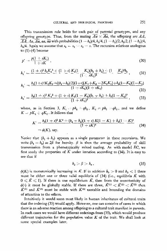
This transmission rule holds for each pair of parental genotypes, and any offspring genotype. Thus, from the mating & x Aa, the offspring are AA, AA, Aa, &, au, Z with probabilities (1 - b&/4, b,/4, (1 - &J/2,6,/2, (1 - &J/4, b,/4. Again we assume that si = sg = sa = s. The recursion relations analogous to (l)-(4) become

k , = (1 + gz b&l2 + (1 + 4 KlU - w4 + a,> + (1 - Jw+J 1

(1 + w2 > (31)

k I = b,(l+s)2K,K,+((6,+6,)/2)(1+s)l~~+K, --2K,K,l+b,(l--K,)(l--K,) 2

(1 + sfG)(l + SK*) (32)

k 3 , = Ml + s12 K22 + (1 + 4 K2(1 - K2)& + 62) + b”(l - w (1 + s&J2 , (33)

where, as in Section 3, K1 = pk, + qk2 , K, = pk, + qk, , and we define K = pK, + $C, . It follows that

K, = b,(l + s)” K2 + (6, + b,)(l + 5) fql - Kf + b,(l - fq2 (1 + SW2 (34)

= WO say.

Notice that (b, + b,) appears as a single parameter in these recursions. We write (b, + b,) as 2,8 for brevity. ,G is then the average probability of skill transmission from a phenotypically mixed mating. As with model EC, we first study the properties of K under iteration according to (34). It is easy to see that if

b, > P > 4, , (35)

4(K) is monotonically increasing in K. If in addition b, > 0 and b, < 1 there must be either one or three valid equilibria of (34) (i.e., equilibria K with 0 < R < 1). If there is one equilibrium &, then from the monotonicity of 4(.) it must be globally stable. If there are three, @) < &?J < &t3) then R(l) and &t3) must be stable with K(2) unstable and bounding the domains of attraction to the others.

Intuitively it would seem most likely in human inheritance of cultural traits that the ordering (35) would apply. However, one can conceive of cases in which there is an adverse reaction among offspring to a cultural trait manifest in parents. In such cases we would have different orderings from (35), which would produce different trajectories for the population value K of the trait. We shall look at some special examples later.


Suppose that {Kt} converges to the equilibrium ri with p bounded away from 0 or 1. Then for sufficiently large t

I Km+, - K,.t+, I EX I K,,, - K,,, I I I y (1 + Sri’)2

(1 + &,tN + SK,,,) ’ (36)

The assumptions then allow us to use the fact that 1 $‘(&)I < 1 to prove that

I K,,,,, - K2.w / + 0 at a geometric rate. The gene frequency ultimately achieved is a function of the initial population array. Both K,,, and K?,, then converge to l?. The net change in the gene frequency is difficult to compute explicitly because we have no expression analogous to (22) for K, .

We now discuss some special cases of model El for which the equilibrium K can be explicitly determined.

Case 1. Additive transmission rule. Assume b, = b, = b, + a, b, === 6, - 201. The possible equilibria are the roots of

sK2 + K[1 - sb, - 24 1 + s)] - 6, = 0.

The positive root &* of (37) is stable, as can be seen from the fact that

If, in particular b, = 0, so that skill is transmitted only in families where at least one parent is skilled, the roots of (37) are

@I) = 0 and R(2) = (24 + s) - 1)/s.

If s > 0, I+’ is globally stable, while if s < 0, K(l) = 0 is globally stable. In the former case the transmission rule interacts with the selective advantage of the skill in preventing the whole population from becoming skilled. In the latter case the selective disadvantage in being skilled overcomes the transmission and the skill is lost from the population. As long as there is some chance that an offspring from a mating in which both parents lack the skill may acquire it from some source (i.e., b, > 0) there will always remain a residual fraction of skill in the population.

Case 2. The Kuru model. Assume that b, = 6, = b, = 1, b, = 0; one member of a mating must be skilled in order that transmission occurs, and transmission is complete. We examine here also the situation where the skill is disadvantageous selectively and call this case “Kurt?’ because of its analogy with the well-known disease endemic in certain New Guinea Tribes. The disease is acquired as a result of the custom of eating or sniffing dead relatives. Some of these dead relatives may carry a virus, which on transmission almost certainly results in the death of the infected member of the tribe. Again we restrict attention to the case of equal genotypic selection which in the Kuru case is most interesting when it is against those who have adopted the custom and have the virus. In our terminology, these are the skilled individuals.


The three equilibria can be explicitly obtained and are J?(l) = I, @) = 0, I@) = -(l + 2s)/s2. Th us, if s < -l/2, three valid equilibria are possible. 4(K) is monotonic; R U) = 1 is always stable and R(s) = 0 is stable provided J?(a) is valid, i.e., s < -l/2. The trait will spread through the population at a rapid rate even if it is deleterious (to the extent that s > -l/2). A more realistic treatment would then have to make allowance for the finite size of the population and the associated possibility of extinction. If s < -l/2 then @a) divides the range of &, values into a lower set, which eventuates in the loss of the skill from the system, and an upper region from which the whole population will eventually become skilled.

From the general convergence argument above we then infer that Kl and Kz both converge to the equilibrium l? value and that p, + p, , which in this case seems difficult to obtain in closed form.

Remark. One interesting aspect of the Kuru model is its relation to the possibility of three interior equilibria for K. In fact if b, is small and positive, and b, is slightly less than 1, leaving 6, and 6, both at unity, three valid interior equilibria exist for s large and negative. The largest and smallest of these will be stable. Necessary conditions in terms of all four parameters can be given for the existence of three roots from the equilibrium cubic equation. These conditions turn out to be difficult to interpret.

7. MODELS WITHOUT SELECTION

mre first return to the system (l)-(4) with sr = sa = s3 = 0. The gene frequency then remains at its initial value p through all subsequent generations. If we write k, as the column vector (k,,, , k,,, , k3,t)T then

k tfl = a + Pkt (39)

where a is the column vector (1 - n, , 1 - n, , 1 - n,)’ and p is the matrix.

(% - WPCI (% - Nl)(l - PO) 0 p = hi - m po n2 - N2 __--

2 +2 ; %L (1 - p,) .

0 (n3 -2N3)Po (n3 - N3N -P,)

1 This model is formally equivalent to that of Cavalli-Sforza and Feldman (1973) where the entries (ni - NJ correspond to 2bi in our previous terminology. The eigenvalues of p are less than unity in absolute value and

kt e CT - PI-l a, where I is the identity matrix.


A more interesting example, without selection, is that of Section 6. Here again p, remains at its initial value p, but now (30), (31), and (32) are replaced by the simpler system

4 = b, + 2w3 - b,) + &“(b3 + bo - W), (3la)

k2’ = 4l + K + K,)(P - b,) + Jw,(b, + b, - W), (32a)

ji31 = 4, + K&3 - h,) + fQ(b, + 4, - V). (33a)

Again, there is change in the average frequency of the skill in the population. In fact, (34) becomes

K-1 = 4, + 2&(B - 4,) + K,z(b, + h, - 39

= f(G), say, to identify it in this simple case.

(34a)

As in the analysis of Section 6, it is possible to show that j K,,, - K2,1 j --f 0, when t --f co. Hence, &, k,,, , K,,, all approach the value ultimately taken by K. The convergence properties of K are of some interest here. The admissible equilibrium for K is

&- = 1 + 2(h - 8) - AlI2 2(b, + 4, - 2P) ’

where A = [l + 2(b, - p)]” - 4b,,[b, + b, - 2,Ll-J. Now if A < 1 the convergence of Kt to k , is monotonic. If 1 < A < 4 the convergence to k is oscillatory. But if A > 4, the only valid equilibrium of (34a) is unstable. In this case we have shown that there is a stable two-point limit cycle. The points are equilibria of the recursion

K+2 = dKt) = fww (41)

Obviously, two equilibria of (41) are those of (34a). The other two are represented as C, , &- with

e i = -(I + 263 - h,)) It (A - 4P2 33

The points C+ and C- lie on either side of &.. and clearly, f(C+) = C- and f(c-) = c+ . A s e ut 1 ria of (40) they are stable whenever they exist, i.e., q ‘l’b whenever K- is unstable.

The conclusion here is that when A < 4, &, k2,t, k3,t all converge to J?- . If A > 4 these three frequencies tend to equality and to oscillate between C+ and C- . We have represented the situation graphically in Fig. 1, highlighting the parameter region which leads to cycling. This is termed the “chip of oscillation.” It should be pointed out that the condition A > 4 is quite extreme


since A is in fact bounded above by 5. We require 4b,(l - 6.J > 3 and indeed b, < b, . These conditions may seem artificial in most common cases of learning, but they are not so unrealistic in situations where children tend to behave in a manner opposite to the parental norm.

- b3

FIG. 1. The shaded area in the top left depicts the parameter set that results in the

stable two point limit cycle (42). The b oundary surface marked E. , El , E, and Es correspond to the stable equilibria I? = 0, I? = I, I? = (b, + b, - I)/(b, + b, - ba), K = b,,//3, respectively. In the unshaded three-dimensional area, I?- specified by (40) is stable.

A very simple example of direct convergence is given by the specification h, = 0, b, = b, = b, = 1. That is, the skill can be acquired only from the parents, but it is enough that one of the parents knows the skill for all the children to acquire it. Similarly, this specification might describe an infectious disease, where the children get the disease only from one or other or both of the parents, but they get it with probability 1. The recursion (10) becomes

Kt = 1 - (1 - I&,)2 = 1 - (1 - K#,

where K,, is the initial K value. Clearly, Kt converges rapidly to 1. For the more general system (30)-(33) t i is also conceivable that a limit

cycle be established. In fact the system I&+, = $(+(KJ) has five possible equilibria of which three are possible roots of (34) at equilibrium. The other two, under certain conditions would presumably be the points of a two point


cycle. From the special Case 2 above, we might conjecture that under conditions that make all equilibria of (34) unstable, this two point cycle would be stable. The algebra appears to be prohibitive, especially since the stability conditions on the roots of the general cubic have not been delimited.

DISCUSSION

The difficulty of assessing whether a quantitative character (such as an inherited disease) is due to a single gene with incomplete penetrance, or is polygenic in its origin, has been pointed out by many authors (e.g., Edwards, 1960; Smith, 1971; Kidd and Cavalli-Sforza, 1973). Most analyses have been made in terms of one generation transitions of population statistics such as correlations between relatives. To study the long term evolutionary dynamics of such quantitative traits requires the assumption of a fitness function (such as the squared deviation from optimum model of Fisher (1930)) and an “inheritance kernel” describing the phenotypes of the offspring of the possible matings (see, e.g., Slatkin, 1970). The genetic origin of the character does not usually enter into these considerations although the studies of Karlin and Carmelli (1974, 1975) and Carmelli and Karlin (1975) are exceptions in this regard.

In this paper we have considered the simplest form of phenotypic variation, namely, a trait taking two values. Since our motivation here has been the study of cultural evolution, the phenotypes were termed skilled and unskilled. With reference to the study of heritable diseases these might just as well be called “infected” and “uninfected.” The latter dichotomy motivated Wilson (1974) in her statistical study of correlations between relatives for a disease transmitted in much the same way as we have modelled here. Wilson’s central conclusion was that, for diseases transmitted environmentally, such correlations may be very close to those expected under a classical one locus scheme.

Our purpose has been to study the equilibrium dynamics of the frequencies of the phenotypes in the population. In particular we have studied the interaction between natural selection on the phenotype and genetically determined differences in the receptivity of offspring to its transmission.

In the main we have assumed that fitness was determined only by the presence or absence of the trait. (The details of Model G, incorporating genetic differences in the selction on the trait are presently under study). We have concentrated on two models of the learning process. In the former, depicted in Table I, the probability that an offspring acquires the skill is determined by its genotype, and by whether the teaching parent had the skill. The model in Table II describes a learning process unaffected by the offspring genotype but dependent on the phenotypic makeup of both parents.


It might have been predicted that for the former model of transmission with selection independent of genotype, differences in the ability to learn among the genotypes would determine the status of any genetic polymorphism. Reflection might have advanced this reasoning to include consideration of whether the selection favored or disfavored the skill. In fact it turns out that if the skill is advantageous and only skilled teaching parents have skilled offspring (ai = 0) a stable genetic polymorphism is possible only if the heterozygotes are better “learners” than homozygotes. It is somewhat surprising that this “overdominance”in learning ability is not sufficient for the maintenance of a genuinely stable polymorphism. Condition (16a), in fact, shows that, under these conditions, selection must be stronger than an amount determined by the learning probabilities. For example, if (1 - Nr) = (1 - NJ = 0.7 and (1 - N,) = 0.8 are the probabilities in Table I that the respective offspring genotypes be skilled when their teaching parent is skilled, (16a) requires that for a stable polymorphism the advantage s, in favor of skill be greater than l/3. Clearly, (16a) can be a stringent additional requirement to the intuitively expected condition of overdominance in learning ability. It is also surprising that, in these cases, if the skill is disadvantageous, no isolated polymorphism exists, and while the skill disappears from the population, the ultimate gene frequency is governed by a neutral curve of equilibria. One way of interpreting the additional condition (16a) is in terms of an added segregation operation. Selection has to overcome the usual Mendelian segregation, and as well, the phenotypic segregation due to imperfect phenotypic transmission.

The analysis in Section 5 illustrates a further interesting fact. Here, using the transmission set up of Table I, there is completely accurate copying of the teaching parent by all offspring irrespective of genotype. Even if the skill is advantageous, no isolated polymorphism obtains since all genotypes are equivalent. But there may be a substantial change in the gene frequency over time due to initiaI differences among the genotypes in the frequency of the skill. These founder effects, together with selection, may cause large gene frequency changes according to (29).

The learning rule in Table II differs from that in Table I in that (1) the genotypes are not differentiated, and (2) the parental mating phenotype deter- mines the probability of learning. In these cases the gene frequency apparently approaches a point determined by initial frequencies, while the phenotypic proportions within the genotypes converge to an isolated equilibrium value. The Kuru model of Section 6 is interesting in this respect since it shows that a strongly disadvantageous custom can spread through a group provided there is enough pressure on the members of the group to conform to the custom. On the other hand, if a strongly disadvantageous trait can be learned outside the family environment then a low frequency of the trait may be maintained. This is completely analogous to the classical mutation-selection balance of


population genetics. In these cases it would be of considerable interest to introduce the added feature of finite population size in order to consider the problem ecologically, as one of potential extinction or survival of the group.

The models and analysis in Sections 5-7 are not concerned in a direct way with population genetics. Yet it seems plausible that the evolution of any phenotype will result in changes in the frequencies of unrelated genes that were initially nonrandomly distributed among the phenotypic classes.

A brief remark on the reasons for some of the strange mathematical behavior of the models is in order. Referring to Eq. (l)-(4), f or example, the transformation in the gene frequency variable involves a confounded term in the selection coefficients and skill proportions. The latter are of course functions of the gene frequency at earlier time points. We have then a form of frequency dependent selection involving a complex delay phenomenon. It is well known (see, e.g., Crow and Kimura, 1970) that frequency dependent selection may produce cycling and other behavior not found in systems with constant selection.

The type of model represented by (l)-(4) IS not restricted in application to cultural and learned traits or infectious diseases transmitted from parent to child. It could also apply to systems of maternal inheritance such as have been discussed by Watson ( 1959) in relation to the cytoplasmic transmission of “sexratio” in Drosophila bifasciata. An extensive review of the epidemiology of such vector-borne diseases was made by Fine (1974) in the context of what he called “vertical transmission” of infections. Watson’s model would fall into this general category with the added feature of sex-ratio distortion. Our model could also be viewed in these terms as allowing genotypically determined differences in either the viability of infected offspring or their resistance to a vector or both.

ACKNOWLEDGMENT

The authors are grateful to Drs. C. Matessi and G. A. Watterson for their valuable suggestions.

REFERENCES

CARNELLI, D. AND KARLIN, S. 1975. Some population genetic models combining artificial and natural selection pressures. I. One locus theory, Theor. Popul. Biol. 7, 94-122.

CAVALLI~FORZA, L. L. AND FELDMAN, M. W. 1973a. Models for cultural inheritance. I. Group mean and within group variation, Theor. Pop&. Biol. 4, 42-55.

CAVALLI~FORZA, L. L. AND FELDMAN, M. W. 1973b. Cultural versus biological inheritance. Phenotypic transmission from parents to children (a theory of the effect of parental phenotypes on children’s phenotypes), Amer. J. Hum. Genet. 25, 618-637.

EDWARDS, J. H. 1960. The simulation of Mendelism, Acta Genet. Stat. Med. 10, 63-70. FELDMAN, M. W. AND CAVALLI-SFORZA, L. L. 1975. Models for cultural inheritance.

A general linear model, Ann. Hum. Biol. 2, 215-226.


FINE, P. E. M. I974 The epidemiological implications of vertical transmission, Thesis, Univ. of London, Faculty of Medicine.

KARLIN, S. AND CARMELLI, D. 1974. Some population genetic models combining artificial and natural selection pressures, Proc. Nut. Acad. Sci. U.S.A. 71, 4727-4731.

KARLIN, S. AND CARMELLI, D. 1975. Some population genetic models combining artificial and natural selection pressures. II. Two locus theory, Theor. Popul. Biol. 7, 123-148.

KIDD, K. AND CAVALLI-SFORZA, L. L. 1973. An analysis of the genetics of schizophrenia, Sot. Biol. 20, 254-265.

KI~IURA, M. 1965. A stochastic model concerning the maintenance of genetic variability in quantitative characters, Proc. Nat. Acad. Sci. U.S.A. 54, 731-736.

LANDE, R. 1975. A model for the maintenance of genetic variability in polygenic characters under stabilizing selection with Mutation and Linkage, Genet. Res. Camb., to appear.

I,ATTER, B. D. H. 1970. Selection in finite populations with multiple alleles, II. Centripetal selection, mutation and isoallelic variation, Genetics 66, 165-186.

LEWONTIN, R. C. 1974. The analysis of variance and the analysis of causes, Amer. J. Hum. Genet. 26, 40&411.

MORTON, N. E. 1974. Analysis of family resemblance. I. Amer. J. Hum. Genet. 26, 318-330. RAO, D., MORTON, N. E., AND YEE, S. 1974. Analysis of family resemblance. II. Amer. J.

Horn. Genet. 26, 331-359. SLATKIN, M. 1970. Selection and polygenic characters, Proc. Nat. Acad. Sci. U.S.A. 66,

87-93. S~IITH, C. 1971. Discriminating between different modes of inheritance in genetic disease,

Clin. Genet. 2, 303-314. WATSON, G. S. 1959. The cytoplasmic “sex-ratio” Condition in Drosophila, Evolution 4,

256-265. WILSON, S. R. 1974. Simulation of Mendelism by a non-genetic Markov chain model,

Ann. Hztm. Genet. London 38, 225-229.

cultural and biological evolutionary processes, selection...

Documents