cuda lab manual - great lakes consortium for petascale

Summer School 2009: Many-Core Processors for Science and Engineering Applications

Hands-On Labs

Xiao-Long Wu, Nady Obeid, I-Jui Sung

The Research Group

Coordinated Science Laboratory

Department of Electrical and Computer Engineering

University of Illinois at Urbana-Champaign

The purpose of the hands-on labs is to assist a 5-day course that teaches CUDA programming concepts and CUDA programming skills. This manual includes a “Hello World!” introductory lab, followed by several well-known problems like matrix-matrix multiplication, vector reduction, and MRI. The purpose of every lab is to reinforce one or several CUDA programming skills and concepts. To help students learn special performance tuning techniques for CUDA, we added an appendix describing several well-known techniques, such as tiling, loop unrolling, data prefetching, etc.

In order to cater to students with different levels of understanding of CUDA programming, we provide 6 hands-on labs from basic programming know-how to performance tuning. Lab 0, 1.1 and 1.2 are for the first hands-on lab section. Lab 2.1 and 2.2 are for the second lab section. Lab 3.1 and 3.2 are for the third lab section. Most labs are designed with levels of different difficulties. Due to limited time in a hands-on lab section, we ask you that you choose the difficulty level that best fits your programming skills. If you have time, you can take on another level. Here is the table of contents of this manual.

Lab 0: Environment Setup and Hello World...........................................................................3

Lab 1.1: Matrix-Matrix Multiplication...................................................................................5

Lab 1.2: Vector Reduction.......................................................................................................8

Lab 2.1: Matrix-Matrix Multiplication with Tiling and Shared Memory.............................13

Lab 2.2: Vector Reduction with Unlimited Input Elements..................................................16

Lab 3.1: Matrix-Matrix Multiplication with Performance Tuning........................................19

Lab 3.2: MRI with Performance Tuning...............................................................................24

Appendix I: CUDA Performance Tuning Techniques...........................................................28

Appendix II: Useful References............................................................................................31

If you have questions during the lab sections, please raise your hand or post your questions on the discussion boards. The TA’s will assist you as soon as they can.

Please do not distribute this manual without consent. For questions about this manual or its content please contact the Impact research group at the University of Illinois at Urbana-Champaign.

Lab 0: Environment Setup and Hello World


1. Objective

The purpose of this lab is to check your setup environment to make sure you can compile and run CUDA programs. This lab is a must for all students using the NCSA machines for the first time.

2. Preliminary work

Step 1: Use an SSH program to login to ac.ncsa.uiuc.edu, using the training account login and initial password given to you. Upon your first login you will be required to change your own password, which will remain active during the entire workshop. After the system accepts your new password, it will end the current login session, and you will be required to log in again with your new password to gain access. Your home directory can be organized in any way you like. To unpack the SDK framework including the code for all of the lab assignments, execute the unpack command in the directory you would like the SDK to be deployed.

$> tar –zxf ~xiaolong/CUDA_WORKSHOP_UIUC.tgz

Step 2: Please acquire a computation node to run the executable.$> qsub -I -l nodes=1:cuda2.2:ppn=1qsub: waiting for job xxxxx.acm to startqsub: job xxxxx.acm ready

Note: You don't need to request a computation node if you use that node only for editing your source files. Besides, each computation session will expire automatically after 30 minutes. Upon expiration, all your applications on that node will be forced to terminate.

Note: If you are a remote user, we recommend you use an FTP program with the SFTP protocol and your account/password to retrieve the source files on ac.ncsa.uiuc.edu for editing because the network may be unstable and disconnected during lab sections.

Step 3: Go to the lab0 directory and make sure it exists and is populated.$> cd CUDA_WORKSHOP_UIUC/projects/lab0-hello_world

There should be at least two source files.

‧ helloword.cu

‧ helloword_kernel.cu

3


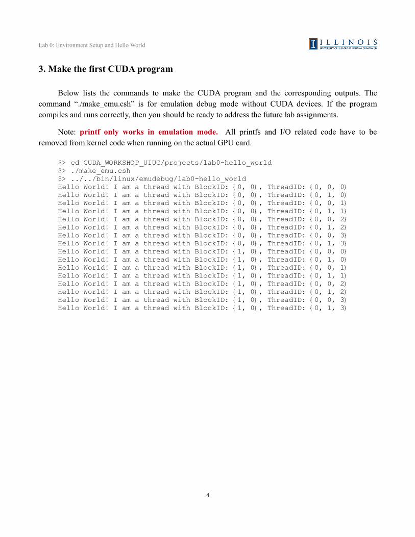
3. Make the first CUDA program

Below lists the commands to make the CUDA program and the corresponding outputs. The command “./make_emu.csh” is for emulation debug mode without CUDA devices. If the program compiles and runs correctly, then you should be ready to address the future lab assignments.

Note: printf only works in emulation mode. All printfs and I/O related code have to be removed from kernel code when running on the actual GPU card.

$> cd CUDA_WORKSHOP_UIUC/projects/lab0-hello_world$> ./make_emu.csh$> ../../bin/linux/emudebug/lab0-hello_worldHello World! I am a thread with BlockID: {0, 0}, ThreadID: {0, 0, 0}Hello World! I am a thread with BlockID: {0, 0}, ThreadID: {0, 1, 0}Hello World! I am a thread with BlockID: {0, 0}, ThreadID: {0, 0, 1}Hello World! I am a thread with BlockID: {0, 0}, ThreadID: {0, 1, 1}Hello World! I am a thread with BlockID: {0, 0}, ThreadID: {0, 0, 2}Hello World! I am a thread with BlockID: {0, 0}, ThreadID: {0, 1, 2}Hello World! I am a thread with BlockID: {0, 0}, ThreadID: {0, 0, 3}Hello World! I am a thread with BlockID: {0, 0}, ThreadID: {0, 1, 3}Hello World! I am a thread with BlockID: {1, 0}, ThreadID: {0, 0, 0}Hello World! I am a thread with BlockID: {1, 0}, ThreadID: {0, 1, 0}Hello World! I am a thread with BlockID: {1, 0}, ThreadID: {0, 0, 1}Hello World! I am a thread with BlockID: {1, 0}, ThreadID: {0, 1, 1}Hello World! I am a thread with BlockID: {1, 0}, ThreadID: {0, 0, 2}Hello World! I am a thread with BlockID: {1, 0}, ThreadID: {0, 1, 2}Hello World! I am a thread with BlockID: {1, 0}, ThreadID: {0, 0, 3}Hello World! I am a thread with BlockID: {1, 0}, ThreadID: {0, 1, 3}

4

Lab 1.1: Matrix-Matrix Multiplication


1. Objective

In the first hands-on lab section, this lab introduces a famous and widely-used example application in the parallel programming field, namely the matrix-matrix multiplication. You will complete key portions of the program in the CUDA language to compute this widely-applicable kernel. In this lab you will learn:

‧ How to allocate and free memory on GPU.

‧ How to copy data from CPU to GPU.

‧ How to copy data from GPU to CPU.

‧ How to measure the execution times for memory access and computation respectively.

‧ How to invoke GPU kernels.

‧ How to write a GPU program doing matrix-matrix multiplication.

Here is the list of the source file directories for lab 1.1. In its initial state, the code does not compile. You must fill in the blanks or lines to make it compile.

Difficulty Level 1: For students with little or no experience of CUDA programming, please choose “projects/lab1.1-matrixmul.1”.

Difficulty Level 2: For students with some experience of CUDA programming, please choose “projects/lab1.1-matrixmul.2”.

2. Modify the given CUDA programs

Step 1: Edit the runTest(…) function in “matrixmul.cu” to complete the functionality of the matrix-matrix multiplication on the host. Follow the comments in the source code to complete these key portions of the host code.

Code segment 1:

‧ Allocate device memory for the input matrices.

‧ Copy the input matrix data from the host memory to the device memory.

‧ Define timer to measure the memory management time.

5


Code segment 2:

‧ Set the kernel launch parameters and invoke the kernel.

‧ Define timer to measure the kernel computation time.

Code segment 3:

‧ Copy the result matrix from the device memory to the host memory.

‧ Define timer to measure the memory management time.

Code segment 4:

‧ Free the device memory.

Step 2: Edit the matrixMul(…) function in “matrixmul_kernel.cu” to complete the functionality of the matrix multiplication on the device. Follow the comments in the source code to complete these key portions of the device code.

Code segment 5:

‧ Define the output index where the thread should output its data.

‧ Iterate over elements in the vectors for the thread’s dot product.

‧ Multiply and accumulate elements of M and N

Step 3: Compile using the provided solution files or Makefiles. Make sure your current directory is under “lab1.1-matrixmul.X”. Simply type the command “./make.csh” (for release mode) to compile the source program, or the command “./make_emu.csh” to compile for emulation debug mode without CUDA devices.

Five test cases are provided for you. They are matrices with size 8 x 8, 128 x 128, 512 x 512, 3072 x 3072, and 4096 x 4096. It’s suggested not to run matrices with sizes larger than 512 x 512 in emulation debug mode. For a matrix with size 3072 x 3072, it takes at least 20 minutes for a CPU to finish. The usage of the executables for release and emulation debug modes are listed below. You can pick only one of the given options, 8, 128, 512, 3072, or 4096.

Run the executable for release mode:$> ../../bin/linux/release/lab1.1-matrixmul <8, 128, 512, 3072, 4096>

Run the executable for emulation debug mode:$> ../../bin/linux/emudebug/lab1.1-matrixmul <8, 128, 512, 3072, 4096>

6


Your output should look like this.

Input matrix file name: Setup host side environment and launch kernel: Allocate host memory for matrices M and N. M: N: Allocate memory for the result on host side. Initialize the input matrices. Allocate device memory. Copy host memory data to device. Allocate device memory for results. Setup kernel execution parameters. # of threads in a block: # of blocks in a grid : Executing the kernel... Copy result from device to host. GPU memory access time: GPU computation time : GPU processing time :

Check results with those computed by CPU. Computing reference solution. CPU Processing time : CPU checksum: GPU checksum: Comparing file lab1.1-matrixmul.bin with lab1.1-matrixmul.gold ... Check ok? Passed.

Record your runtime with respect to different input matrix sizes as follows:

Matrix Size GPU Memory Access Time (ms)

GPU Computation

Time (ms)

GPU Processing Time (ms)

Ratio of Computation Time as compared with matrix 128x128

8 x 8

128 x 128 1

512 x 512

3072 x 3072

4096 x 4096

What do you see from these numbers?

7

Lab 1.2: Vector Reduction


1. Objective

The objective of this lab is to familiarize you with a step often used in scientific computation, reduction. A reduction is combining all elements of an array into a single value using some associative operator. Data-parallel implementations take advantage of this associativity to compute many operations in parallel, computing the result in O(lg N) total steps without increasing the total number of operations performed. One such O(lg N) reduction is the one shown below in Figure 1.1. This reduction has benefits over other reduction patterns, in terms of minimizing thread divergence and coalescing memory accesses.

3 1 7 0 4 1 6 3

7 2 1 3 3 4 1 6 3

2 0 5 1 3 3 4 1 6 3

2 5 5 1 3 3 4 1 6 3

Figure 1.1 Reduction scheme 1, using O(lg N) steps and O(N) computations

What you will learn from this lab:

． How to allocate and free memory on GPU.

． How to copy data from CPU to GPU.

． How to copy data from GPU to CPU.

． How to write a GPU program doing sum reduction

． How to measure the execution time and shared memory bank conflicts using CUDA profiler.

． How different reduction schemes affect bank conflicts

8


Here is the list of the source files for lab 1.2. They should compile completely, although with warnings, as they are.

Difficulty Level 1: For students with little or no experience of CUDA programming, please choose “projects/lab1.2-reduction.1”. This lab does not compile until you fill the blanks or lines.

Difficulty Level 2: For students with some experience of CUDA programming, please choose “projects/lab1.2-reduction.2”. This lab compiles with warnings.

2. Modifying the given CUDA programs

Step 1: Modify the function computeOnDevice(...) defined in vector_reduction.cu.

Code segment 1:

‧ Allocate CUDA device memory.

‧ Copy input data from host memory to CUDA device memory.

‧ Copy results from CUDA device memory back to host memory.

Step 2: In vector_reduction_kernel.cu, modify the kernel function to implement the reduction scheme shown in Figure 1.1. Your implementation should use shared memory to increase efficiency.

Code segment 2:

‧ Load data from global memory to shared memory.

‧ Do sum reduction on the shared memory data.

‧ Store data back to shared memory.

Step 3: Once you have finished the code, simply type the command “./make.csh” (for release mode) in the project directory (lab1.2-reduction.X depending on the difficulty level) to compile the source program, or the command “./make_emu.csh” to compile for emulation debug mode without using CUDA devices.

For release mode, the executable is at:../../bin/linux/release/vector_reduction

For emulation debug mode, the executable is at:../../bin/linux/emudebug/vector_reduction

There are two operation modes for this application, as listed below. The only difference is the input to both GPU and CPU versions of reduction code. Thereafter, the GPU version code will be launched first, followed by the CPU version code as a gold reference. The results generated by both versions will be compared to see if there is any discrepancy. If the discrepancies are within a certain

9


tolerance threshold (caused by the different execution orders in sequential by CPU version or in parallel by GPU version), it will print out "Test Passed" and the reduction results of both GPU and CPU versions. Otherwise, “Test Failed” will be printed out.

No arguments: The program will create a randomly initialized array as the input to both the GPU and CPU versions of reduction code. Below is an example.$> ../../bin/linux/release/vector_reduction

One argument: The program will use the specified data file as the input to both GPU and CPU versions of reduction code. A test case, “data.txt”, is provided for you. You can modify it as your new test cases. Below is an example.$> ../../bin/linux/release/vector_reduction data.txt

Note that this lab does not provide running time information. Because the test case size is very small, the CPU running time will outperform GPU running time. Your output should look like this.

Test PASSEDdevice: host: Input vector: random generated.

Step 4: Now that you have implemented the reduction scheme depicted in Figure 1.1, we will compare this implementation with two other reduction schemes. Please edit the function reduction(…) in “vector_reduction_kernel.cu”, where two reduction schemes are left for you to implement, as listed in Figure 1.2 and 1.3. Figure 1.2 is one reduction scheme in which each thread is responsible for the addition of two adjacent nodes in the distance of power of 2 for each operation level. Figure 1.3 is another reduction scheme in which each thread is handling the addition of two nodes in the distances from n-1 to 1. For example, in the first operation level, the 1st thread adds the 1st and the 8th elements. Hence the distance between the two nodes are 8-1 = 7. The 2nd threads adds the 2nd and the (8-1)th elements. The corresponding distance is 7-2 = 5. And the distances for the nodes added by 3rd and 4th

theads are 6-3 = 2 and 5-4 = 1, respectively.

Note the regular access patterns in the two reductions schemes. Most applications, use regular operation patterns to eliminate redundant branch divergences and bank conflicts.

10


3 1 7 0 4 1 6 3

4 1 7 0 5 1 9 3

1 1 1 7 0 1 4 1 9 3

2 5 1 7 0 1 4 1 9 3

Figure 1.2 Reduction scheme 2

3 1 7 0 4 1 6 3

6 7 8 4 4 1 6 3

1 0 1 5 8 4 4 1 6 3

2 5 1 5 8 4 4 1 6 3

Figure 1.3 Rreduction scheme 3

Step 5: Once you have finished all the code, use the following command to enable the CUDA profiler (assuming bash is used) when executing your program. The command launchs the CUDA profiler with the given profiler configuration file, profile_config, under the same project directory.

$> CUDA_PROFILE=1 CUDA_PROFILE_CONFIG=./profile_config \ ../../bin/linux/release/vector_reduction

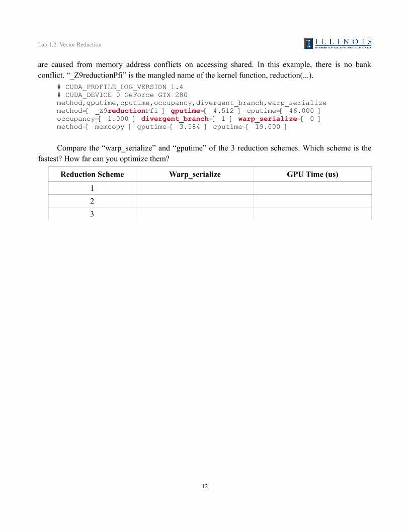
The default output file for the CUDA profiler is cuda_profile.log. Below is an example. “gputime” shows the micro-seconds it took for a CUDA function to execute. “warp_serialize” refers the number of threads in a warp executed serially, in other words, the number of bank conflicts, which

11


are caused from memory address conflicts on accessing shared. In this example, there is no bank conflict. “_Z9reductionPfi” is the mangled name of the kernel function, reduction(...).

# CUDA_PROFILE_LOG_VERSION 1.4# CUDA_DEVICE 0 GeForce GTX 280method,gputime,cputime,occupancy,divergent_branch,warp_serializemethod=[ _Z9reductionPfi ] gputime=[ 4.512 ] cputime=[ 46.000 ] occupancy=[ 1.000 ] divergent_branch=[ 1 ] warp_serialize=[ 0 ] method=[ memcopy ] gputime=[ 3.584 ] cputime=[ 19.000 ]

Compare the “warp_serialize” and “gputime” of the 3 reduction schemes. Which scheme is the fastest? How far can you optimize them?

Reduction Scheme Warp_serialize GPU Time (us)

1

2

3

12

Lab 2.1: Matrix-Matrix Multiplication with Tiling and Shared Memory

Lab 2.1: Matrix-Matrix Multiplication with Tiling and Shared

Memory

1. Objective

This lab is an enhanced matrix-matrix multiplication, which uses the features of shared memory and synchronization between threads in a block. The device shared memory is allocated for storing the sub-matrix data for calculation, and threads share memory bandwidth which was overtaxed in previous matrix-matrix multiplication lab. In this lab you will learn:

‧ How to apply tiling on matrix-matrix multiplication.

‧ How to use shared memory on the GPU.

‧ How to apply thread synchronization in a block.

Here is the list of the source file directories for lab 2.1. In its initial state, the code does not compile. You must fill in the blanks or lines to make it compile.

Difficulty Level 1: For students with little or no experience of CUDA programming, please choose “projects/lab2.1-matrixmul.1”.

Difficulty Level 2: For students with some experience of CUDA programming, please choose “projects/lab2.1-matrixmul.2”.

Difficulty Level 3: For students with good experience of CUDA programming, please choose “projects/lab2.1-matrixmul.3”.

2. Modifying the given CUDA programs

Step 1: Edit the matrixMul(…) function in matrixmul_kernel.cu to complete the functionality of the matrix-matrix multiplication on the device. The host code has already been completed for you. The source code need not be modified elsewhere.

Code segment 1: Determine the update values for the tile indices in the loop.

Code segment 2: Implement matrix-matrix multiplication inside a tile.

Code segment 3: Store the data back to global memory.

13


Step 2: Compile using the provided solution files or Makefiles. Make sure your current directory is under “lab2.1-matrixmul.X”. Simply type the command “./make.csh” (for release mode) to compile the source program, or the command “./make_emu.csh” to compile for emulation debug mode without CUDA devices.

Five test cases are provided to you. They are matrices with size 8 x 8, 128 x 128, 512 x 512, 3072 x 3072, and 4096 x 4096. It is not recommend that you run matrices with sizes larger than 512 x 512 in emulation debug mode. For a matrix with size 3072 x 3072, it takes at least 20 minutes for a CPU to finish. The usage of the executables for release and emulation debug modes are listed below. You can pick only one of the given options, 8, 128, 512, 3072, or 4096.

Run the executable for release mode:$> ../../bin/linux/release/lab2.1-matrixmul <8, 128, 512, 3072, 4096>

Run the executable for emulation debug mode:$> ../../bin/linux/emudebug/lab2.1-matrixmul <8, 128, 512, 3072, 4096>


Input matrix file name: Setup host side environment and launch kernel: Allocate host memory for matrices M and N. M: N: Allocate memory for the result on host side. Initialize the input matrices. Allocate device memory. Copy host memory data to device. Allocate device memory for results. Setup kernel execution parameters. # of threads in a block: # of blocks in a grid : Executing the kernel... Copy result from device to host. GPU memory access time: GPU computation time : GPU processing time :


14


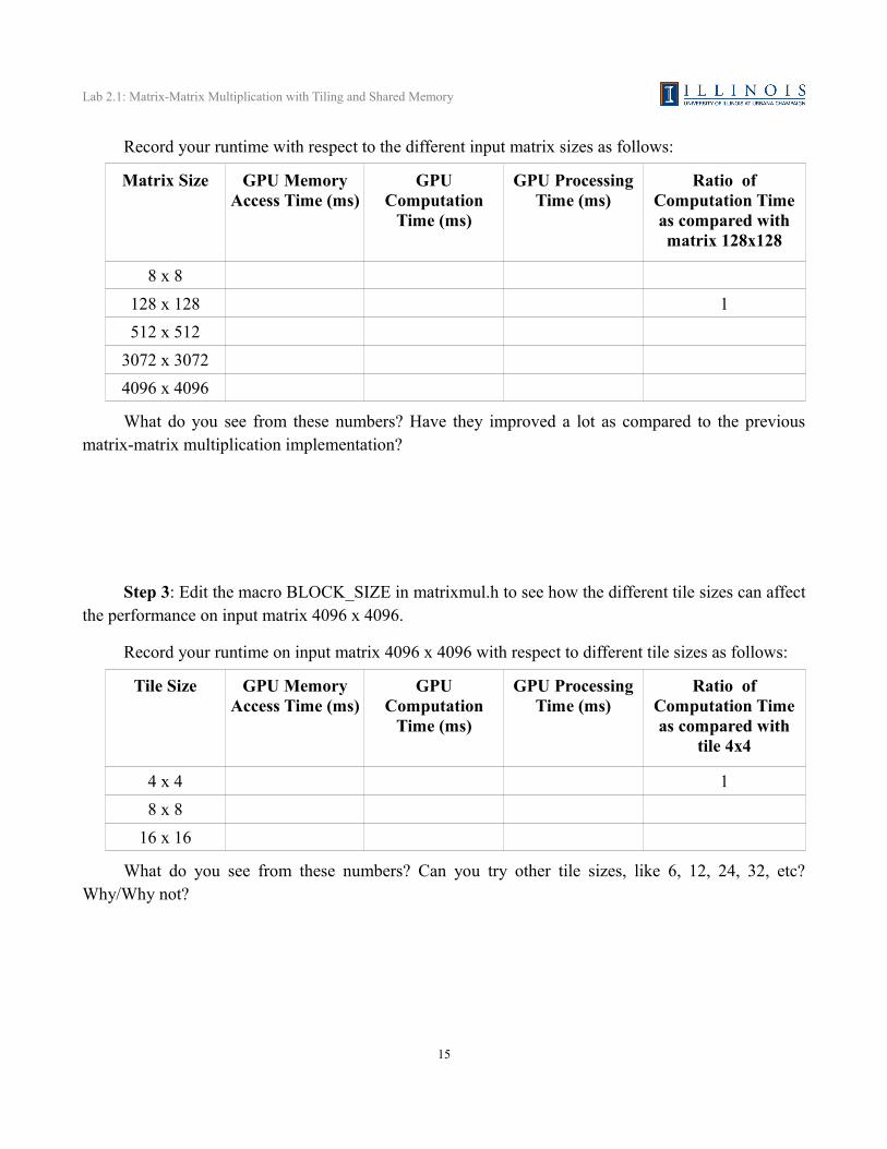
Record your runtime with respect to the different input matrix sizes as follows:

Matrix Size GPU Memory Access Time (ms)

GPU Computation

Time (ms)


Ratio of Computation Time as compared with matrix 128x128

8 x 8

128 x 128 1

512 x 512

3072 x 3072

4096 x 4096

What do you see from these numbers? Have they improved a lot as compared to the previous matrix-matrix multiplication implementation?

Step 3: Edit the macro BLOCK_SIZE in matrixmul.h to see how the different tile sizes can affect the performance on input matrix 4096 x 4096.

Record your runtime on input matrix 4096 x 4096 with respect to different tile sizes as follows:

Tile Size GPU Memory Access Time (ms)

GPU Computation

Time (ms)


Ratio of Computation Time as compared with

tile 4x4

4 x 4 1

8 x 8

16 x 16

What do you see from these numbers? Can you try other tile sizes, like 6, 12, 24, 32, etc? Why/Why not?

15

Lab 2.2: Vector Reduction with Unlimited Input Elements


1. Objective

This lab is an generalized implementation of sum reduction, which is able to handle arbitrary input sizes. In this lab you wil learn:

‧ How to use multiple kernel invocations as a means of synchronization between thread blocks in dividing-and-conquering large problems.

‧ How to measure the performance of a CUDA program.

‧ Techniques for handling non-power-of-two problem sizes.

Here is a list of the source file directories for lab 2.2. They should compile completely, although with warnings, as they are.

Difficulty Level 1: For students with little or no experience of CUDA programming, please choose “projects/lab2.2-reduction.1”.

Difficulty Level 2: For students with some experience of CUDA programming, please choose “projects/lab2.2-reduction.2”.


Step 1: Edit the runTest(…) function in reduction_largearray.cu, to complete the functionality of the host code.

Code segment 1:

‧ Define timer and kernel synchronization call to measure the kernel execution time.

Step 2: Modify the function reductionArray(...) defined in reduction_largearray_kernel.cu to complete the functionality of a kernel that can handle the input of any size. Note that this lab requires synchronization between thread blocks so you need to invoke the kernel multiple times. Each kernel handles only lg(BLOCK_SIZE) steps in the overall reduction process. You can use the output array to store intermediate results. The final sum should be stored in array element zero to be compared with the gold sum.

There are two aspects to this lab that can be dealt with seperately: 1) handling an array size that is not a multiple of BLOCK_SIZE, and 2) handling arrays that are too large to fit in one block. It is advisable to start with the first requirement.

In order to regularize the input data size, one technique that is often used is to pad the array with

16


trailing zero elements when loading into shared memory, in order to have as many elements as there are threads in a block.

Afterwards, you can modify the host function reductionArray(...) to handle large input sizes. You will most likely need to use a loop to reduce the array through multiple kernel calls or to use recursive kernel function calls. Both are doable. One way to debug your code is to copy data back to the host after each reduction level and analyzing it for correctness. Note that to be able to handle large sizes that are not multiple of BLOCK_SIZE, you need to make sure you allocate, at every level of the reduction, enough blocks to cover the entire input, even if the last block has less than BLOCK_SIZE elements. For instance, for a BLOCK_SIZE of 4 and an array size of 10, you will need to generate three blocks, not two.

Step 3: Once you have finished writing the code, simply type the command “./make.csh” (for release mode) in the project directory (lab2.2-reduction.X depending on the difficulty level) to compile the source program, or the command “./make_emu.csh” to compile for emulation debug mode without using CUDA devices.

For release mode, the executable is at:../../bin/linux/release/reduction_largearray

For emulation debug mode, the executable is at:../../bin/linux/emudebug/reduction_largearray

The program will create a randomly initialized array as the input to both GPU and CPU versions of reduction code. The size of this array is specified in the macro DEFAULT_NUM_ELEMENTS defined in reduction_largearray.cu. The default size is 16,000,000. You can run the compiled executable using the following command.

$> ../../bin/linux/release/vector_reduction

The GPU version reduction will be launched first, followed by the CPU version as a gold reference. The results generated by both versions will be compared to see if there is any discrepancy. If the discrepancies are within a certain tolerance threshold (caused by the different execution orders in sequential by CPU version or in parallel by GPU version), it will print out "Test PASSED" and the reduction results of both GPU and CPU versions. Otherwise, “Test FAILED” will be printed out.

17


Your output should look like this.Using device 0: GeForce GTX 280

**===-------------------------------------------------===**Processing 16000000 elements...Host CPU Processing time: CUDA Processing time: Speedup: Test PASSEDdevice: host:

Step 4: Plot the speedup you measured with different input sizes. At what size of input will your CUDA kernel be faster than the CPU one?

Input Size CPU Processing Time (ms) GPU Processing Time (ms)

At what size of input will the speedup factor of your CUDA kernel over CPU implementation start to saturate?

18

Lab 3.1: Matrix-Matrix Multiplication with Performance Tuning

Lab 3.1: Matrix-Matrix Multiplication with Performance

Tuning

1. Objective

This lab provides more flexibility for you to tune the matrix multiplication performance. You can give different values for loop unrolling degree, tiling factors and working size, and turn on/off the spill and prefetch functions to see the performance differences.

You can examine the source code in matrixmul.cu and matrixmul_kernel.cu and see how these switches are applied to the source code. The given programs are correct. You should be able to compile them without errors. In this lab you will learn how to use the following optimization techniques:

‧ Tiling.

‧ Loop unrolling.

‧ Varying the working size.

‧ Register spilling.

‧ Data prefetching.

‧ How to use CUDA profiler to profile your CUDA program.

‧ How to get the memory usage information of your CUDA program.

The source files for lab 3.1 are in “projects/lab3.1-matrixmul”, and should compile completely and correctly as they are.


Step 1: Edit the preprocessor definitions in matrixmul.h to vary the kernel optimization parameters. The source code does not need to be edited elsewhere. The project is correct as given, and should compile without errors.

Step 2: Compile using the provided solution files or Makefiles. Make sure your current directory is under “lab3.1-matrixmul”. Simply type the command “./make.csh” (for release mode) will compile the source program, or the command “./make_emu.csh” to compile for emulation debug mode without CUDA devices.

The test case given for this lab is a matrix with size 4096 x 4096. The usage of the executables for release and emulation debug modes are listed below.

19


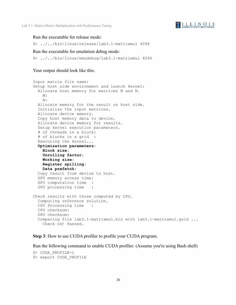
Run the executable for release mode:$> ../../bin/linux/release/lab3.1-matrixmul 4096

Run the executable for emulation debug mode:$> ../../bin/linux/emudebug/lab3.1-matrixmul 4096


Input matrix file name: Setup host side environment and launch kernel: Allocate host memory for matrices M and N. M: N: Allocate memory for the result on host side. Initialize the input matrices. Allocate device memory. Copy host memory data to device. Allocate device memory for results. Setup kernel execution parameters. # of threads in a block: # of blocks in a grid : Executing the kernel... Optimization parameters: Block size: Unrolling factor: Working size: Register spilling: Data prefetch: Copy result from device to host. GPU memory access time: GPU computation time : GPU processing time :


Step 3: How to use CUDA profiler to profile your CUDA program.

Run the following command to enable CUDA profiler: (Assume you're using Bash shell)$> CUDA_PROFILE=1$> export CUDA_PROFILE

20


Run the executable again. You will notice a file named, “cuda_profile.log”, under the same project directory. Below is a log example. The bold red words are the things you should look for. “gputime” shows the micro-seconds it takes for a CUDA function, e.g., matrixMul(...). “occupancy” shows the ratio of active warps to the maximum number of warps supported on a multiprocessor of the GPU. On G80, the maximum number of warps is 768/32 = 24 and each multiprocessor has 8192 32-bit registers. In GTX 280, the maximum active warps is 1024/32=32 and the number of registers per SM is 16384. The number of active warps will be limited by the number of registers and shared memory needed by a block. For more information about these specifications, please refer to Appendix A of “NVIDIA CUDA Programming Guide Version 2.1”.

$> ../../bin/linux/release/lab3.1-matrixmul 4096$> cat cuda_profile.log# CUDA_PROFILE_LOG_VERSION 1.4# CUDA_DEVICE 0 GeForce GTX 280method,gputime,cputime,occupancymethod=[ memcopy ] gputime=[ 24041.824 ] cputime=[ 38837.000 ]method=[ memcopy ] gputime=[ 24577.951 ] cputime=[ 38641.000 ]method=[ _Z9matrixMulPfS_S_ii ] gputime=[ 1109786.625 ] cputime=[ 10.000 ] occupancy=[ 0.500 ]method=[ memcopy ] gputime=[ 46265.602 ] cputime=[ 108240.000 ]

Step 4: How to get the memory usage information for your CUDA program.

Run the program, “find_mem_usage.csh”, with the following commands under the same project directory. The output file matrixmul.cu.cubin lists the profile of the CUDA program on the usage of registers, local memory, shared memory, constant memory, etc. For this lab, no constant memory is used so it's not listed in the output file.

$> ./find_mem_usage.csh matrixmul.cunvcc -I. -I../../common/inc -I/usr/local/cuda/include -DUNIX -o matrixmul.cu.cubin -cubin matrixmul.cu See matrixmul.cu.cubin for register usage.

$> head -n 20 matrixmul.cu.cubinarchitecture {sm_10}abiversion {1}modname {cubin}code { name = _Z9matrixMulPfS_S_ii lmem = 0 smem = 2084 reg = 9 bar = 1 const { … }…

21


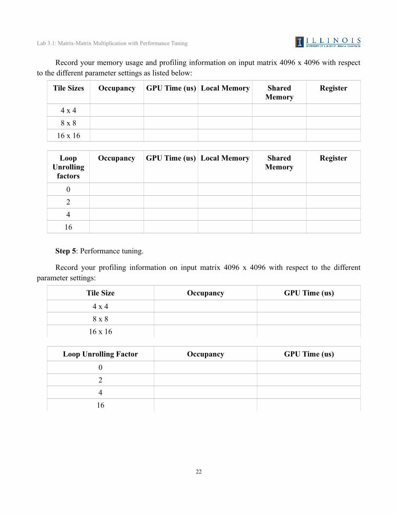
Record your memory usage and profiling information on input matrix 4096 x 4096 with respect to the different parameter settings as listed below:

Tile Sizes Occupancy GPU Time (us) Local Memory Shared Memory

Register

4 x 4

8 x 8

16 x 16

Loop Unrolling

factors

Occupancy GPU Time (us) Local Memory Shared Memory

Register

0

2

4

16

Step 5: Performance tuning.

Record your profiling information on input matrix 4096 x 4096 with respect to the different parameter settings:

Tile Size Occupancy GPU Time (us)

4 x 4

8 x 8

16 x 16

Loop Unrolling Factor Occupancy GPU Time (us)

0

2

4

16

22


Working Size Occupancy GPU Time (us)

1

2

4

Register Spilling Occupancy GPU Time (us)

Disabled

Enabled

Prefetching Occupancy GPU Time (us)

Disabled

Enabled

Can you find the parameter combination that gets the best performance? Record the best performance you can achieve, and try to explain why the selection of parameters you chose was a good one.

Parameters Setting/Results

Tile Sizes

Loop Unrolling Factors

Working Sizes

Register Spilling

Prefetching

Occupancy

GPU Time (us)

23

Lab 3.2: MRI with Performance Tuning


1. Objective

The objective of this lab is to tune the performance of an existing MRI image reconstruction kernel. You will do so by using constant memory where possible, improving SM occupancy by changing the block size, using registers for data that is reused often, etc.

Here is the list of the source file directories for lab 3.2. The project is correct as given, and should compile completely and correctly without errors as they are.

Difficulty Level 1: For students with little experience of CUDA programming, please choose “projects/lab3.2-mriQ.1”.

Difficulty Level 2: For students with good experience of CUDA programming, please choose “projects/lab3.2-mriQ.2”.


Step 1 for Difficulty Level 1: Edit the preprocessor definitions in computeQ.h to vary the kernel optimization parameters. You can give different values for loop unrolling degree and block size, and turn on/off the if condition simplification, the constant memory usage, and the trigonometry optimization to see the performance differences. The source code does not need to be edited elsewhere.

Step 1 for Difficulty Level 2: Edit the source code in computeQ.cu to improve the performance of the application. To help you get started, it would be useful for you to know that the kernel computeQ_GPU takes the most time to execute and has the highest speedup potential than all other kernels. Some techniques you should consider:

‧ Using constant memory for read-only data.

‧ Changing the number of threads per block to improve thread utilization on an SM.

‧ Loading in registers data that is frequently reused.

‧ Unrolling “for” loops to decrease code branching.

‧ Simplifying conditional statements where possible.

‧ Though this is not always applicable, and is not covered in the lectures, in this particular application, it will be beneficial to use the function sincosf( ) (google it).

The source code does not need to be edited elsewhere.

24


Step 2: Compile using the provided solution files or Makefiles. Make sure your current directory is under “lab3.2-mriQ.X”. Simply type the command “./make.csh” (for release mode) will compile the source program, or the command “./make_emu.csh” to compile for emulation debug mode without CUDA devices.

Run the executable for release mode:$> ../../bin/linux/release/mri-q -S -i data/sutton.sos.Q64x147258.input.float -o my_output.out

Run the executable for emulation debug mode:$> ../../bin/linux/emudebug/mri-q -S -i data/sutton.sos.Q64x147258.input.float -o my_output.out

You output should look like this:2097152 pixels in output; 147258 samples in trajectory; using samplesIO: GPU: Copy: Compute:

To verify the correctness of the output, you can compare it to the reference that we have given you, by typing the following command in the project directory:

$> diff -s my_output.out data/reference_full.out

Your output should look like this.Files my_output.out and data/reference_full.out are identical

Note: Since the runtime of the full data set may take up to 3 minutes, you can experiment with smaller data sets. We have given you the reference files for 512 and 10000 samples to compare your output against.

To run the program with 512 samples:$> ../../bin/linux/release/mri-q -S -i \ data/sutton.sos.Q64x147258.input.float -o my_output 512

To run the program with 10000 samples:$> ../../bin/linux/release/mri-q -S -i \ data/sutton.sos.Q64x147258.input.float -o my_output 10000

25


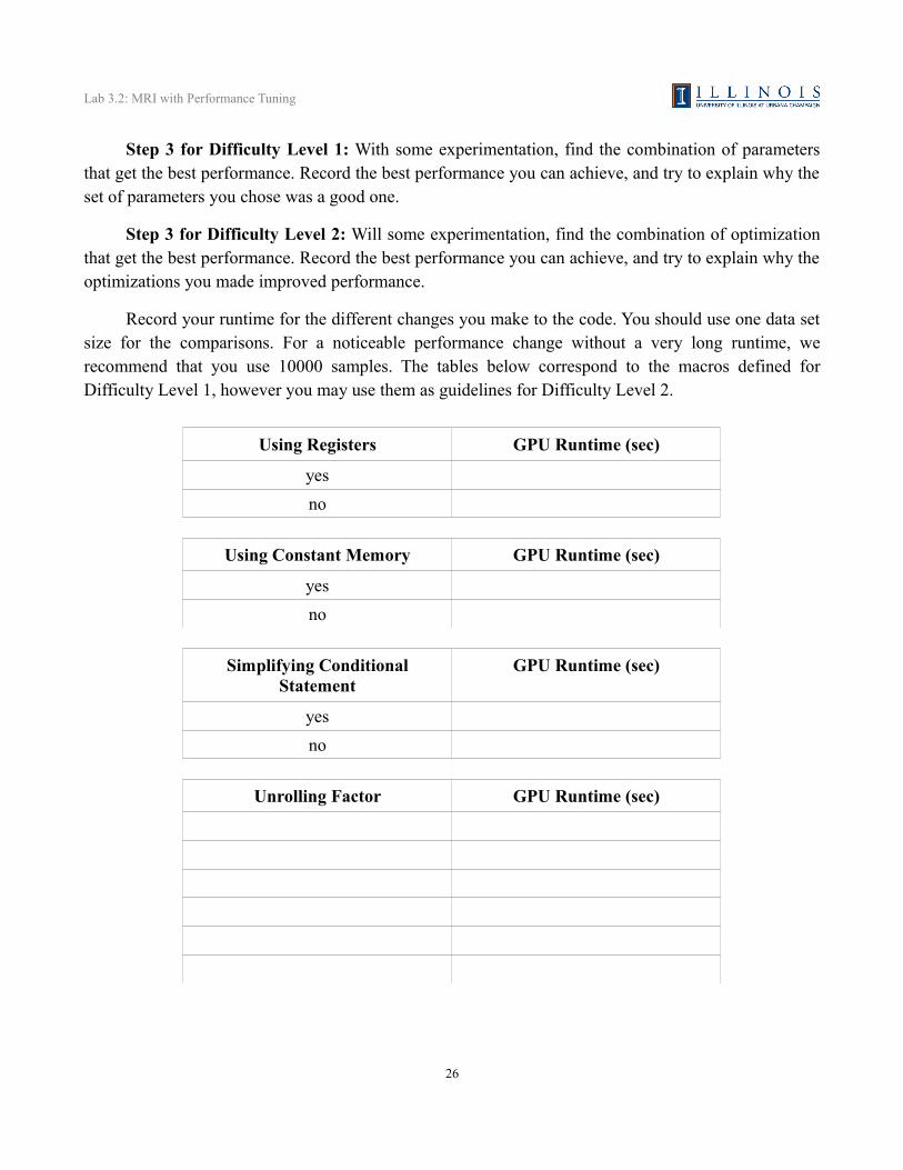
Step 3 for Difficulty Level 1: With some experimentation, find the combination of parameters that get the best performance. Record the best performance you can achieve, and try to explain why the set of parameters you chose was a good one.

Step 3 for Difficulty Level 2: Will some experimentation, find the combination of optimization that get the best performance. Record the best performance you can achieve, and try to explain why the optimizations you made improved performance.

Record your runtime for the different changes you make to the code. You should use one data set size for the comparisons. For a noticeable performance change without a very long runtime, we recommend that you use 10000 samples. The tables below correspond to the macros defined for Difficulty Level 1, however you may use them as guidelines for Difficulty Level 2.

Using Registers GPU Runtime (sec)

yes

no

Using Constant Memory GPU Runtime (sec)

yes

no

Simplifying Conditional Statement

GPU Runtime (sec)

yes

no

Unrolling Factor GPU Runtime (sec)

26


Block Size GPU Runtime (sec)

Trigonometry Optimization GPU Runtime (sec)

yes

no

27

Appendix I: CUDA Performance Tuning Techniques


In this appendix we define some common tuning techniques used to improve the performance of CUDA programs. Note that these techniques may not work for all types of applications, and in some cases may even hinder performance. Whenever you make an optimization, you have to keep in mind register usage, memory accessing, thread occupancy on an SM, etc.

1. Tiling

A tile refers to the working set of data operated on by an entity. A tile can refer to the input data and/or output data of an entity. An entity can be a block, grid, warp, etc. The following situations show how increasing or decreasing the tile size can improve the performance.

‧ Increasing the output tile size can improve the input data reuse in shared memory, if increasing the output tile size does not cause the input size to become large enough to affect thread occupancy on an SM.

‧ If the data are too big to put into shared memory, it is useful to shrink the tile size in order to make it fit, thus taking advantage of the high speed shared memory and reducing bandwidth to global memory.

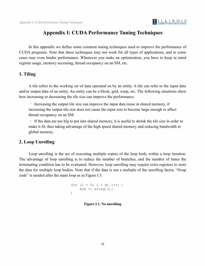
2. Loop Unrolling

Loop unrolling is the act of executing multiple copies of the loop body within a loop iteration. The advantage of loop unrolling is to reduce the number of branches, and the number of times the terminating condition has to be evaluated. However, loop unrolling may require extra registers to store the data for multiple loop bodies. Note that if the data is not a multiple of the unrolling factor, “fixup code” is needed after the main loop as in Figure I.3.

for (i = 0; i < N; i++) { sum += array[i];}

Figure I.1. No unrolling

28


for (i = 0; i < N; i=i+2) { sum += array[i]; sum += array[i+1];}

Figure I.2. Unrolling by a factor of 2 when the number of loop iterations is a multiple of 2

for (i = 0; i < N-1; i=i+2) { sum += array[i]; sum += array[i+1];}if (N mod 2 != 0) sum += array[N-1];}

Figure I.3. Unrolling by a factor of 2 with fixup code

3. Working Size

Working size is the amount of work done per thread. Usually refers to the number of input or output elements each thread computes for.

4. Register Spilling

Register spilling is when the programmer uses shared memory as extra register space to relieve real register usage. Since the number of registers per SM is limited, any extra registers needed by the kernel are automatically spilled to local memory by the compiler. Since local memory has high latency as global memory, it is beneficial for performance if the programmer manually spills extra registers to the shared memory, if shared memory space is available.

5. Data Prefetching

Data prefetching, as the name suggests, is to fetch data in advance. It's often used to fetch data for the next loop iteration. The benefit of prefetching data is to leverage the asynchronous aspect of memory accesses in CUDA. When a memory access operation is executed, it does not block other operations following it as long as they don't use the data from the operation. As written in Figure I.4, every addition waits for its data to be loaded from memory. Inside the loop of Figure I.5, the device first launches a memory load operation for the next iteration and does an addition in parallel. The time

29


for the addition is actually overlapping with the memory access time. But the increased register usage may lower the number of active warps on an SM.

for (i = 0; i < N; i++) { sum += array[i];}

Figure I.4. Kernel without prefetching

temp = array[0];for (i = 0; i < N-1; i++) { temp2 = array[i+1]; sum += temp; temp = temp2;}sum += temp;

Figure I.5. Kernel with prefetching

6. Using Registers

Using registers to store frequently reused data can save memory bandwidth and memory access latency, thus improving the kernel performance. In Figure I.6, arrays v1 and v2 are stored in global memory. They make (N*M)+(N*M) memory load requests. But we can see array v1 is reused M times in the inner-most loop. Therefore we can use a register “temp”, as shown in Figure I.7, to eliminate redundant memory loads of v1 elements. The new number of total memory loads is N+(N*M).

for (k = 0; k < N; i++){ for (i = 0; i < M; i++) { sum += v1[k]*v2[i]; }}

Figure I.6. Kernel without register usage

for (k = 0; k < N; i++){ temp = v1[k]; for (i = 0; i < M; i++) { sum += temp*v2[i]; }}

Figure I.7. Kernel with register usage

30

Appendix II: Useful References

Appendix II: Useful References

Here lists the useful documents and links about CUDA programming.

The first course talking about CUDA programming in the world.

‧ http://courses.ece.illinois.edu/ece498/al/

The official CUDA programming manual by NVIDIA, describing the programming model, CUDA program syntax, performance tuning guidelines, technical specifications about CUDA devices, etc.

‧ NVIDIA CUDA Programming Guide Version 2.1

Useful CUDA materials maintained by the Impact Research Group at UIUC

‧ https://edcharles.engin.umich.edu/trac/virtual_school/wiki/CudaIndex

NVIDIA CUDA Zone, a place to raise your questions to senior CUDA programmers and NVIDIA engineers.

‧ http://forums.nvidia.com/index.php?showforum=71

31

cuda lab manual - great lakes consortium for petascale

Documents