ct6 cmp upgrade 2013 2014 - actuarial education … upgrade/ct6-pu-14.pdfthis cmp upgrade lists all...
TRANSCRIPT

CT6: CMP Upgrade 2013/14 Page 1
The Actuarial Education Company © IFE: 2014 Examinations
Subject CT6
CMP Upgrade 2013/14
CMP Upgrade This CMP Upgrade lists all significant changes to the Core Reading and the ActEd material since last year so that you can manually amend your 2013 study material to make it suitable for study for the 2014 exams. It includes replacement pages and additional pages where appropriate. Alternatively, you can buy a full replacement set of up-to-date Course Notes at a significantly reduced price if you have previously bought the full price Course Notes in this subject. Please see our 2014 Student Brochure for more details.
This CMP Upgrade contains: All non-trivial changes to the Syllabus objectives and Core Reading. Changes to the ActEd Course Notes, Question and Answer Bank, and Series X
Assignments that will make them suitable for study for the 2014 exams.

Page 2 CT6: CMP Upgrade 2013/14
© IFE: 2014 Examinations The Actuarial Education Company
1 Changes to the Syllabus objectives and Core Reading
1.1 Syllabus objectives There have been no changes to the syllabus.
1.2 Core Reading Chapter 2 Page 10 The following paragraph has been deleted. It is often convenient to express this result in terms of the value of a statistic,
such as X , rather than the sample values X. So, for example,
( )f XqΩ = ( ) ( )
( )
f X f
f X
q qΩ.
In practice these are equivalent. Chapter 3 Page 4 In Section 1.1, where the exponential distribution is defined, it has been specified that > 0l and > 0x .
Page 5 In Section 1.2, where the gamma distribution is defined, it has been specified that
> 0a , > 0l and > 0x .
Page 7
In Section 2.1, where the Pareto distribution is defined, it has been specified that > 0a , > 0l and > 0x .

CT6: CMP Upgrade 2013/14 Page 3
The Actuarial Education Company © IFE: 2014 Examinations
Page 10 Under the section on Method of Moments, ix has been redefined:
xi = the ith value in the sample Page 11 In Section 2.3, where the Weibull distribution is defined, it has been specified that > 0c , > 0g and > 0x .
Page 16 The section on MLE has been modified to include formulae for the discrete case. A replacement page is provided. Page 19 In the first paragraph of Core Reading, references to estimates have been changed to estimators. Page 20 In the first paragraph of Core Reading, references to estimates have been changed to estimators. In Section 3.6, the word n-denominator has been inserted before sample variance. Pages 27 to 30 Various changes have been made to the section on mixture distributions, to help improve the flow. Replacement pages are provided.
Page 4 CT6: CMP Upgrade 2013/14
© IFE: 2014 Examinations The Actuarial Education Company
Chapter 4 Pages 6 and 7 There have been several modifications to Pages 6 and 7, including a deletion of the discussion on complete and incomplete integrals. Replacement pages are provided. Page 8 Some alterations have been made to the notation used in the discussion of the reinsurer’s conditional claims distribution. A replacement page is provided. Page 10 The second and third paragraphs of Core Reading have been altered. A replacement page is provided. Pages 19 and 20 The following passage has been deleted: The same device as the one used to obtain (1.3) can be used to convert (3.1) to a complete integral. (3.1) can be written as
E(Y) = • • •
- +Ú Ú Ú0 / /( ) ( ) ( )
M k M kkx f x dx kx f x dx M f x dx
= k E(X) k •
-Ú /( / ) ( ) .
M kx M k f x dx
The new mean amount paid by the insurer is
E(Y) = •
- +Ú0( ( ) ( / ) ).k E X y f y M k dy (3.2)
Note that the integral in (3.2) has the same form as that in (1.3). Page 20 The paragraph of Core Reading in the middle of the page has been replaced with: One important general point that can be made is that the new mean claim amount paid by the insurer is not k times the mean claim amount paid by the insurer without inflation.
CT6: CMP Upgrade 2013/14 Page 5
The Actuarial Education Company © IFE: 2014 Examinations
Page 24 Some alterations have been made to the discussion on estimation. A replacement page is provided. Chapter 7 Page 18 At the bottom of the page, the following fragment of a sentence has been deleted: and the distribution of S follows that of N. Pages 19 to 24 Some alterations have been made to the discussion of the compound Poisson distribution and the result concerning the sum of compound Poisson distributions. Replacement pages are provided. Pages 24 to 26 In the discussion on the compound binomial distribution, the distribution of the number of claims has been changed from N ~ bin(n, q) to the more usual N ~ bin(n, p) so that all of the q’s are now p’s and vice-versa. Replacement pages are provided. Chapter 8 Page 3 The second paragraph has been rewritten as: If, for example, ~ ( )N Poi l , SI has a compound Poisson distribution with Poisson
parameter , and the thi individual claim amount is Yi. Similarly, SR has a
compound Poisson distribution with Poisson parameter , and the thi individual claim amount is Zi.

Page 6 CT6: CMP Upgrade 2013/14
© IFE: 2014 Examinations The Actuarial Education Company
Pages 5 and 6 Some small changes have been made to the example in the Core Reading to improve the flow. Replacement pages are provided. Pages 6 and 8 Some changes have been made to the notation used for the PDF of the reinsurer’s conditional claims distribution, to tie in with the changes made to the notation in Chapter 4. Replacement pages are provided. Page 11 Two-thirds of the way down the page, a sentence has been rewritten as: Thus, the distribution of Yj is compound binomial, with individual claim amount
random variable Xj.
At the bottom of the page, the following sentence has been deleted: It was seen in Section 3.5 of Chapter 7 that there is no general result about the distribution of such a sum. Page 13 The first part of Section 3.2 has been altered to: Consider a portfolio consisting of n independent policies. The aggregate claims from the i-th policy are denoted by the random variable Si, where Si has a
compound Poisson distribution with parameters i , and the CDF of the
individual claim amounts distribution is F(x). Notice that, for simplicity, the CDF of the distribution of individual claim amounts, F(x), is assumed to be identical for all the policies. In this example the distribution of individual claim amounts, ie F(x), is assumed to be known but the values of the Poisson parameters, ie the i s, are not known.
CT6: CMP Upgrade 2013/14 Page 7
The Actuarial Education Company © IFE: 2014 Examinations
Page 17 The first part of Section 3.4 has been altered to: Now a different example is considered. Suppose, as before, there is a portfolio of n policies. The aggregate claims from a single policy have a compound Poisson distribution with parameters , and the CDF of the individual claim amounts random variable is F(x). The Poisson parameters are the same for all policies in the portfolio.
Chapter 11 The origin years in the run-off triangles have been brought more up-to-date. This doesn’t affect the understanding of the material in anyway so we have not provided replacement pages.
Page 8 CT6: CMP Upgrade 2013/14
© IFE: 2014 Examinations The Actuarial Education Company
2 Changes to the ActEd Course Notes All Chapters The Summary and Formulae Pages have been updated for all chapters in an attempt to better reflect the key material to be revised for the exam. Replacement pages are provided for all chapters. Chapter 2 Page 10 The following paragraph has been deleted:
The notation can get a little confusing here. Remember that X is a sample mean, whereas X refers to the whole group of values of X ie a vector containing all the
values in the sample.
Chapter 3 Page 17 The 1st step in the description of how to find an MLE has been modified to take account of the discrete case: (1) Write down the likelihood function for the available data. If the likelihood is
based on a set of known values x x xn1 2, , , , then the likelihood function will take
the form 1 2( ) ( ) ( )nf x f x f x , where f x( ) is the PDF of X where X is a
continuous random variable (or ( ) ( ) ( )1 2 nP X x P X x P X x= = = in the case
where X is a discrete random variable).
Chapter 4 Pages 6 and 7 There have been several modifications to Pages 6 and 7 to try and improve the clarity, including the deletion of Questions 4.3 and 4.4. Replacement pages are provided.
CT6: CMP Upgrade 2013/14 Page 9
The Actuarial Education Company © IFE: 2014 Examinations
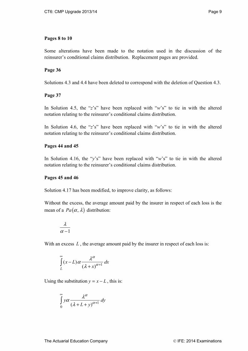
Pages 8 to 10 Some alterations have been made to the notation used in the discussion of the reinsurer’s conditional claims distribution. Replacement pages are provided. Page 36 Solutions 4.3 and 4.4 have been deleted to correspond with the deletion of Question 4.3. Page 37 In Solution 4.5, the “z’s” have been replaced with “w’s” to tie in with the altered notation relating to the reinsurer’s conditional claims distribution. In Solution 4.6, the “z’s” have been replaced with “w’s” to tie in with the altered notation relating to the reinsurer’s conditional claims distribution. Pages 44 and 45 In Solution 4.16, the “y’s” have been replaced with “w’s” to tie in with the altered notation relating to the reinsurer’s conditional claims distribution. Pages 45 and 46 Solution 4.17 has been modified, to improve clarity, as follows: Without the excess, the average amount paid by the insurer in respect of each loss is the
mean of a ( ),Pa a l distribution:
1
la -
With an excess L , the average amount paid by the insurer in respect of each loss is:
1
( )( )L
x L dxx
a
ala
l
•
+-+Ú
Using the substitution y x L= - , this is:
1
0 ( )y dy
L y
a
ala
l
•
++ +Ú
Page 10 CT6: CMP Upgrade 2013/14
© IFE: 2014 Examinations The Actuarial Education Company
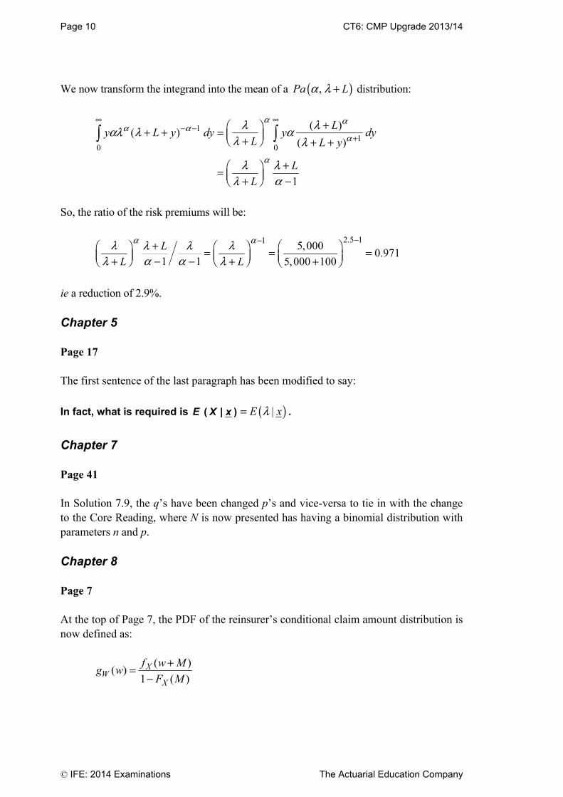
We now transform the integrand into the mean of a ( ),Pa La l + distribution:
11
0 0
( )( )
( )
1
Ly L y dy y dy
L L y
L
L
a aa a
a
a
l lal l al l
l ll a
• •- -
++Ê ˆ+ + = Á ˜Ë ¯+ + +
+Ê ˆ= Á ˜Ë ¯+ -
Ú Ú
So, the ratio of the risk premiums will be:
2.5 11 5,000
0.9711 1 5,000 100
L
L L
a al ll la al l
--+ Ê ˆÊ ˆ Ê ˆ= = =Á ˜ Á ˜ Á ˜Ë ¯ Ë ¯ Ë ¯- -+ + +
ie a reduction of 2.9%. Chapter 5 Page 17 The first sentence of the last paragraph has been modified to say:
In fact, what is required is ( | )E X x ( )|E xl= .
Chapter 7 Page 41 In Solution 7.9, the q’s have been changed p’s and vice-versa to tie in with the change to the Core Reading, where N is now presented has having a binomial distribution with parameters n and p. Chapter 8 Page 7 At the top of Page 7, the PDF of the reinsurer’s conditional claim amount distribution is now defined as:
( )
( )1 ( )
XW
X
f w Mg w
F M
+=-

CT6: CMP Upgrade 2013/14 Page 11
The Actuarial Education Company © IFE: 2014 Examinations
Chapter 10 Significant changes have been made to the ActEd notes for this chapter to improve the explanations and examples. Replacement pages are provided for the whole chapter. Chapter 11 The origin years in the run-off triangles have been brought more up-to-date. This doesn’t affect the understanding of the material in anyway so we have not provided replacement pages. Page 11 We have added the following paragraphs to the top of Page 11, before Question 11.7 to help explain the general statistical model: Note that some of the terminology above is being used in a different context to previously. The development factors jr in this general statistical model are defined
differently to the development factors that we have met previously. The development factors that we met previously were used to project forward cumulative claims data. The development factors in the general statistical model are being used to model incremental data. They are defined above as the proportion of claims from a particular accident year that are paid in the jth development year. As such, they are a set of factors that add up to 1. A question may help you to see what is going on.

Page 12 CT6: CMP Upgrade 2013/14
© IFE: 2014 Examinations The Actuarial Education Company
3 Changes to the Q&A Bank Part 2 Questions Question 2.10 The headings in the table have been corrected to j , jY and jP .
(Previously these were incorrectly labelled as i , iY and iP .)
Solution 2.21 Two formulae were incorrectly labelled ( )E Y . These have now been changed to ( )E Z .
CT6: CMP Upgrade 2013/14 Page 13
The Actuarial Education Company © IFE: 2014 Examinations
4 Changes to the X Assignments
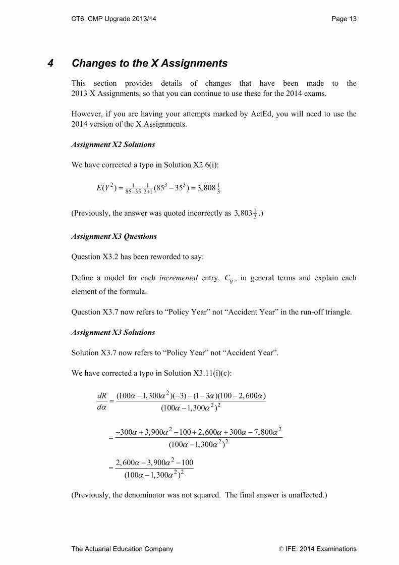
This section provides details of changes that have been made to the 2013 X Assignments, so that you can continue to use these for the 2014 exams. However, if you are having your attempts marked by ActEd, you will need to use the 2014 version of the X Assignments. Assignment X2 Solutions We have corrected a typo in Solution X2.6(i):
2 3 31 1 185 35 2 1 3( ) (85 35 ) 3,808E Y - += - =
(Previously, the answer was quoted incorrectly as 133,803 .)
Assignment X3 Questions Question X3.2 has been reworded to say: Define a model for each incremental entry, ijC , in general terms and explain each
element of the formula. Question X3.7 now refers to “Policy Year” not “Accident Year” in the run-off triangle. Assignment X3 Solutions Solution X3.7 now refers to “Policy Year” not “Accident Year”. We have corrected a typo in Solution X3.11(i)(c):
2
2 2
(100 1,300 )( 3) (1 3 )(100 2,600 )
(100 1,300 )
dR
d
2 2
2 2
2
2 2
300 3,900 100 2,600 300 7,800
(100 1,300 )
2,600 3,900 100
(100 1,300 )
(Previously, the denominator was not squared. The final answer is unaffected.)

Page 14 CT6: CMP Upgrade 2013/14
© IFE: 2014 Examinations The Actuarial Education Company
Assignment X4 Solutions We have corrected a typo in the notes (in italics) to solution X4.2:
2 20.005
2
200
10
zn >
(Previously, the subscript of the z was 0.01.) We have added the following new statement (worth [1] mark) to Solution X4.4(i): This reproducibility removes the variability of using different sets of random numbers, which is helpful for comparing different models. Any two of the three statements are now needed to score a maximum of [2] marks on this part.

CT6: CMP Upgrade 2013/14 Page 15
The Actuarial Education Company © IFE: 2014 Examinations
5 Other tuition services In addition to this CMP Upgrade you might find the following services helpful with your study.
5.1 Study material We offer the following study material in Subject CT6:
ASET (ActEd Solutions with Exam Technique) and Mini-ASET
Flashcards
Mock Exam A and Additional Mock Pack (AMP)
Revision Notes
Online Classroom. For further details on ActEd’s study materials, please refer to the 2014 Student Brochure, which is available from the ActEd website at www.ActEd.co.uk.
5.2 Tutorials We offer the following tutorials in Subject CT6:
a set of Regular Tutorials (lasting two or three full days)
a Block Tutorial (lasting two or three full days)
a Revision Day (lasting one full day)
a Taught Course (lasting four full days)
a series of webinars (lasting approximately an hour and a half each)
CT6 Online Classroom. For further details on ActEd’s tutorials, please refer to our latest Tuition Bulletin, which is available from the ActEd website at www.ActEd.co.uk.

Page 16 CT6: CMP Upgrade 2013/14
© IFE: 2014 Examinations The Actuarial Education Company
5.3 Marking You can have your attempts at any of our assignments or mock exams marked by ActEd. When marking your scripts, we aim to provide specific advice to improve your chances of success in the exam and to return your scripts as quickly as possible. For further details on ActEd’s marking services, please refer to the 2014 Student Brochure, which is available from the ActEd website at www.ActEd.co.uk.

CT6: CMP Upgrade 2013/14 Page 17
The Actuarial Education Company © IFE: 2014 Examinations
6 Feedback on the study material
ActEd is always pleased to get feedback from students about any aspect of our study programmes. Please let us know if you have any specific comments (eg about certain sections of the notes or particular questions) or general suggestions about how we can improve the study material. We will incorporate as many of your suggestions as we can when we update the course material each year. If you have any comments on this course please send them by email to [email protected] or by fax to 01235 550085.

© IFE: 2014 Examinations The Actuarial Education Company
All study material produced by ActEd is copyright and is sold for the exclusive use of the purchaser. The copyright is owned
by Institute and Faculty Education Limited, a subsidiary of the Institute and Faculty of Actuaries.
Unless prior authority is granted by ActEd, you may not hire out, lend, give out, sell, store or transmit electronically or
photocopy any part of the study material.
You must take care of your study material to ensure that it is not used or copied by anybody else.
Legal action will be taken if these terms are infringed. In addition, we may seek to take disciplinary action through the
profession or through your employer.
These conditions remain in force after you have finished using the course.

CT6-01: Decision theory Page 25
The Actuarial Education Company IFE: 2014 Examinations
Chapter 1 Summary Zero-sum games In this chapter we study zero-sum two-player games. If we call our players (who are in conflict) Alice and Bob then the term zero-sum tells us that whatever Alice loses, Bob must win; there are no payments to or receipts from third parties. Both Alice and Bob have a number of different strategies open to them. The payoffs from each combination of strategies can be represented in a matrix. The payoffs associated with Alice’s available strategies (labelled I, II, III, etc) determine the columns of the matrix. The payoffs associated with Bob’s available strategies (labelled 1, 2, 3, etc) determine the rows of the payoff matrix. One strategy is said to dominate another if the first strategy is at least as good as the second and in some cases better. Dominated strategies can always be discarded. Problems in Decision Theory usually involve the determination of optimum strategies and the corresponding payoff, or value, of the game. Two criteria that are often used to determine optimum strategies are the minimax criterion and the Bayes criterion. Under the minimax criterion, all players will adopt the strategy that minimises their maximum loss (or maximises their minimum gain). The minimax criterion can be thought of as a ‘best-of-all-evils’ approach. A saddle point is the name given to an entry of a payoff matrix that is the largest in its column and the smallest in its row. If a saddle point exists then each player will adopt the pure strategy, with the options that correspond to the saddle point being chosen. If there is no saddle point, a randomised strategy can be adopted to enable a player to minimise his/her maximum expected loss. This means that the player will vary his or her choice of strategy in a random fashion but in accordance with some fixed set of probabilities. Statistical games A statistical game can be regarded as a game between nature (which controls the relevant features of a population) and the statistician (who is trying to make a decision about the population).

Page 26 CT6-01: Decision theory
IFE: 2014 Examinations The Actuarial Education Company
An example of a statistical game is where a statistician wishes to determine whether a coin is fair (F) or biased (B) towards tails, with nature acting as his/her “opponent”. A decision function sets out the action for the statistician to take based on each outcome of an event, eg the event might be a single toss of the coin and one example of a decision function is: F if the coin toss results in heads and B if the coin toss results in tails. A risk function sets out the expected loss for a particular decision function and a given actual state of nature. In order to calculate the expected loss, probabilities must be assigned to each state of nature. The statistician can then use the minimax criterion to find the decision function that minimises the maximum value of risk function ... ... or the Bayes criterion to find the decision function that minimises the expected value of the risk function.

CT6-02: Bayesian statistics Page 27
The Actuarial Education Company IFE: 2014 Examinations
Chapter 2 Summary Bayesian estimation vs classical estimation A common problem in statistics is to estimate the value of some unknown parameter . The classical approach to this problem is to treat as a fixed, but unknown, constant and use sample data to estimate its value. For example, if represents some population mean then its value may be estimated by a sample mean. The Bayesian approach is to treat as a random variable. Prior distribution of θ
The prior distribution of represents the knowledge available about the possible values
of before the collection of any sample data. The prior PDF of q is denoted ( )f q .
Likelihood function of the sample data A likelihood function is then determined, based on a set of observations
( )1 2, , ... , nx x x x= . The likelihood function is just the same as the joint density (or, in
the discrete case, the joint probability) of X X Xn1 2, , , | . However, the likelihood is
considered to be a function of rather than one of x x xn1 2, , , . Since we are
assuming that the random variables X X n1| , , | are independent, the joint density
function f x x xX n| ( , , , ) 1 2 is equal to the product of the individual density functions
f xX ii |( ) . The likelihood function is therefore:
( ) |1
| ( )i
n
X ii
L x f xqq=
=’
Posterior distribution of θ
The PDF (or probability function) of the prior distribution and the likelihood function are then combined to obtain the PDF (or probability function) of the posterior distribution for .
Page 28 CT6-02: Bayesian statistics
IFE: 2014 Examinations The Actuarial Education Company
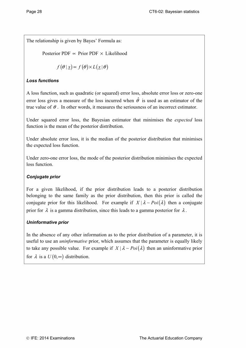
The relationship is given by Bayes’ Formula as: Posterior PDF μ Prior PDF ¥ Likelihood
( ) ( ) ( )| |f x f L xq q qμ ¥
Loss functions A loss function, such as quadratic (or squared) error loss, absolute error loss or zero-one
error loss gives a measure of the loss incurred when q is used as an estimator of the true value of q . In other words, it measures the seriousness of an incorrect estimator. Under squared error loss, the Bayesian estimator that minimises the expected loss function is the mean of the posterior distribution. Under absolute error loss, it is the median of the posterior distribution that minimises the expected loss function. Under zero-one error loss, the mode of the posterior distribution minimises the expected loss function. Conjugate prior For a given likelihood, if the prior distribution leads to a posterior distribution belonging to the same family as the prior distribution, then this prior is called the
conjugate prior for this likelihood. For example if ( )|X Poil l then a conjugate
prior for l is a gamma distribution, since this leads to a gamma posterior for l . Uninformative prior In the absence of any other information as to the prior distribution of a parameter, it is useful to use an uninformative prior, which assumes that the parameter is equally likely
to take any possible value. For example if ( )|X Poil l then an uninformative prior
for l is a ( )0,U • distribution.
CT6-02: Bayesian statistics Page 28a
The Actuarial Education Company IFE: 2014 Examinations
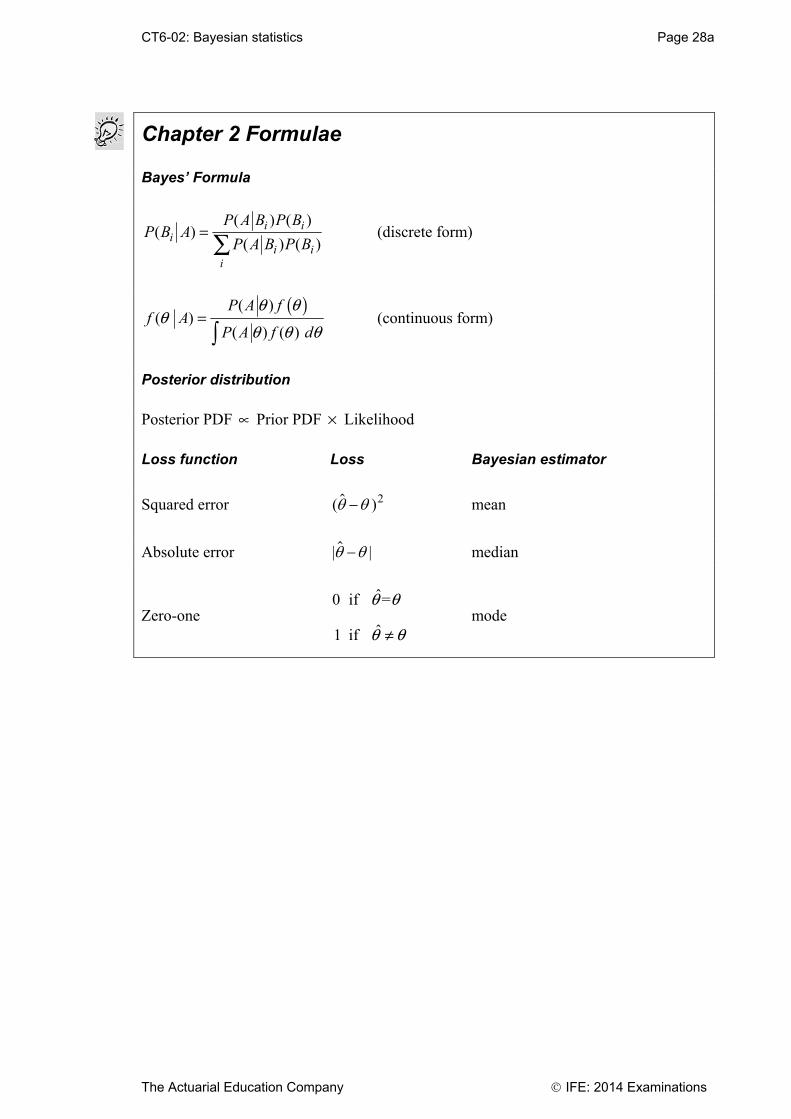
Chapter 2 Formulae Bayes’ Formula
( ) ( )( )
( ) ( )=Â
i ii
i ii
P A B P BP B A
P A B P B (discrete form)
( )( )( )
( ) ( )=Ú
P A ff A
P A f d
q qq
q q q (continuous form)
Posterior distribution Posterior PDF μ Prior PDF ¥ Likelihood Loss function Loss Bayesian estimator
Squared error ( ) 2 mean
Absolute error | | median
Zero-one ˆ0 if =
ˆ1 if
q q
q qπ mode

Page 28b CT6-02: Bayesian statistics
IFE: 2014 Examinations The Actuarial Education Company
This page has been left blank so that you can keep the chapter summaries together as a revision tool.

CT6-03: Loss distributions Page 15
The Actuarial Education Company IFE: 2014 Examinations
3 Estimation
The methods of maximum likelihood, moments and percentiles can be used to fit distributions to sets of data. The fit of the distribution can be tested formally by
using a 2 test. The method of percentiles is outlined in Section 3.7; the other
methods and the 2 test have been covered in Subject CT3, Probability and
Mathematical Statistics. The formulae for the densities, the moments and the moment generating functions (where they exist) for the distributions discussed in this chapter are given in the Formulae and Tables for Actuarial Examinations. We will give a brief summary of the method of moments and of maximum likelihood estimation for those students who have not taken Subject CT3 recently. An example of using the chi square distribution will also be given, in case you have forgotten how to carry out this test.
3.1 The method of moments
For a distribution with r parameters, the moments are as follows:
jm = =Â
1
1 nji
i
xn
j = 1, 2 … r
where jm = E(Xj), a function of the unknown parameter, , being estimated
n = the sample size xi = the ith value in the sample
The estimate for the parameter, , can be determined by solving the equation above. Where there is more than one parameter, they can be determined by solving the simultaneous equations for each mj.
To obtain a method of moments estimator for a parameter, we equate the corresponding sample and population non-central moments. So, for example, if we were trying to estimate the value of a single parameter, and we had a sample of n claims whose sizes were x x xn1 2, , , , we would solve the equation:
1
1( )
n
ii
E X xn =
= Â
ie we would equate the first non-central moments for the population and the sample.
Page 16 CT6-03: Loss distributions
IFE: 2014 Examinations The Actuarial Education Company
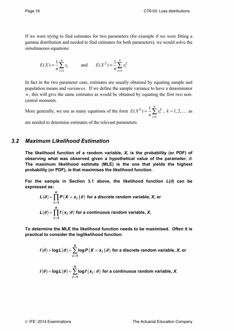
If we were trying to find estimates for two parameters (for example if we were fitting a gamma distribution and needed to find estimates for both parameters), we would solve the simultaneous equations:
1
1( )
n
ii
E X xn =
= Â and 2 2
1
1( )
n
ii
E X xn =
= Â
In fact in the two parameter case, estimates are usually obtained by equating sample and population means and variances. If we define the sample variance to have a denominator n , this will give the same estimates as would be obtained by equating the first two non-central moments.
More generally, we use as many equations of the form 1
1( )
nk k
ii
E X xn =
= Â , k 1 2, , as
are needed to determine estimates of the relevant parameters.
3.2 Maximum Likelihood Estimation
The likelihood function of a random variable, X, is the probability (or PDF) of observing what was observed given a hypothetical value of the parameter, . The maximum likelihood estimate (MLE) is the one that yields the highest probability (or PDF), ie that maximises the likelihood function. For the sample in Section 3.1 above, the likelihood function L() can be expressed as:
( ) ( )=
= =’1
|n
ii
L P X xq q for a discrete random variable, X, or
( ) ( )|=
=’1
n
ii
L f xq q for a continuous random variable, X.
To determine the MLE the likelihood function needs to be maximised. Often it is practical to consider the loglikelihood function:
( ) ( ) ( )=
= = =Â1
log log |n
ii
l L P X xq q q for a discrete random variable, X, or
( ) ( ) ( )=
= = Â1
log logn
ii
l L f xq q q for a continuous random variable, X.
CT6-03: Loss distributions Page 17
The Actuarial Education Company IFE: 2014 Examinations
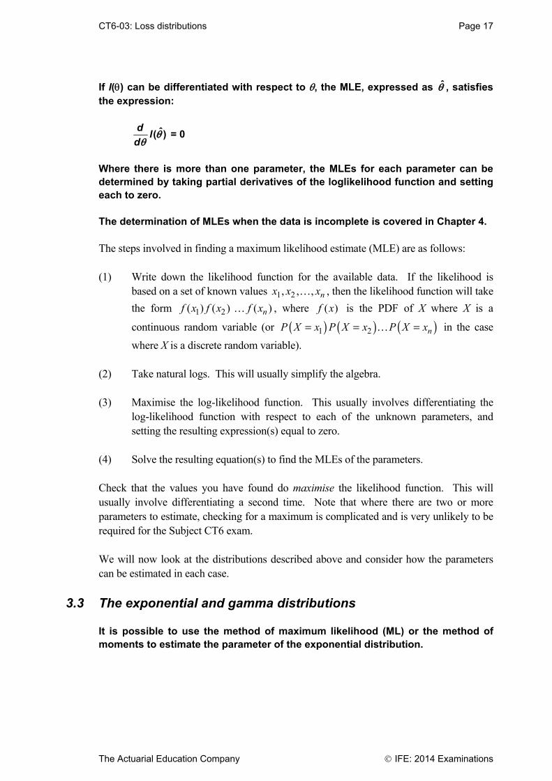
If l() can be differentiated with respect to , the MLE, expressed as q , satisfies the expression:
ˆ( )d
ld
= 0
Where there is more than one parameter, the MLEs for each parameter can be determined by taking partial derivatives of the loglikelihood function and setting each to zero. The determination of MLEs when the data is incomplete is covered in Chapter 4. The steps involved in finding a maximum likelihood estimate (MLE) are as follows: (1) Write down the likelihood function for the available data. If the likelihood is
based on a set of known values x x xn1 2, , , , then the likelihood function will take
the form 1 2( ) ( ) ( )nf x f x f x , where f x( ) is the PDF of X where X is a
continuous random variable (or ( ) ( ) ( )1 2 nP X x P X x P X x= = = in the case
where X is a discrete random variable). (2) Take natural logs. This will usually simplify the algebra. (3) Maximise the log-likelihood function. This usually involves differentiating the
log-likelihood function with respect to each of the unknown parameters, and setting the resulting expression(s) equal to zero.
(4) Solve the resulting equation(s) to find the MLEs of the parameters. Check that the values you have found do maximise the likelihood function. This will usually involve differentiating a second time. Note that where there are two or more parameters to estimate, checking for a maximum is complicated and is very unlikely to be required for the Subject CT6 exam. We will now look at the distributions described above and consider how the parameters can be estimated in each case.
3.3 The exponential and gamma distributions
It is possible to use the method of maximum likelihood (ML) or the method of moments to estimate the parameter of the exponential distribution.
Page 18 CT6-03: Loss distributions
IFE: 2014 Examinations The Actuarial Education Company
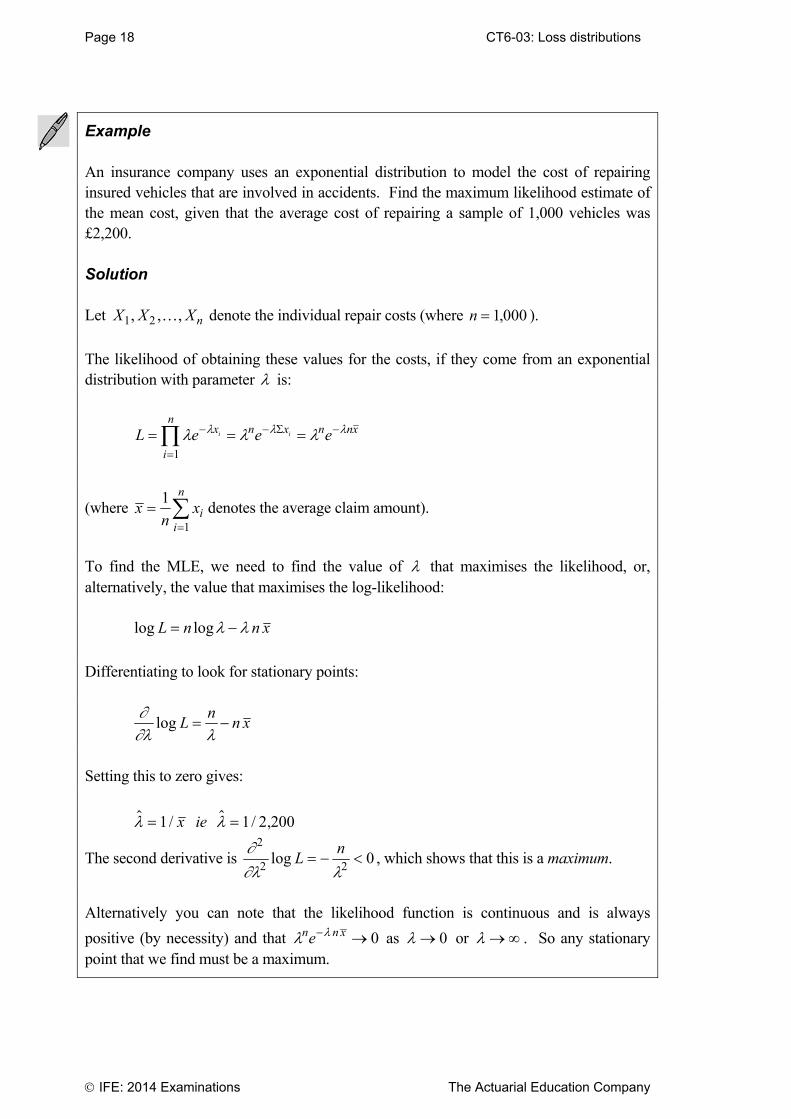
Example An insurance company uses an exponential distribution to model the cost of repairing insured vehicles that are involved in accidents. Find the maximum likelihood estimate of the mean cost, given that the average cost of repairing a sample of 1,000 vehicles was £2,200. Solution Let X X Xn1 2, , , denote the individual repair costs (where n 1 000, ).
The likelihood of obtaining these values for the costs, if they come from an exponential distribution with parameter is:
L e e ex
i
nn x n nxi i
1
(where xn
xii
n
1
1
denotes the average claim amount).
To find the MLE, we need to find the value of that maximises the likelihood, or, alternatively, the value that maximises the log-likelihood:
log logL n n x
Differentiating to look for stationary points:
log Ln
n x
Setting this to zero gives:
/ 1 x ie / , 1 2 200
The second derivative is
2
2 20log L
n , which shows that this is a maximum.
Alternatively you can note that the likelihood function is continuous and is always
positive (by necessity) and that n n xe 0 as 0 or . So any stationary point that we find must be a maximum.
CT6-03: Loss distributions Page 27
The Actuarial Education Company IFE: 2014 Examinations
5 Mixture distributions
The exponential distribution is one of the simplest models for insurance losses. Suppose that each individual in a large insurance portfolio incurs losses according to an exponential distribution. What we’re thinking of here is that the amounts of Mr Ferrari’s insurance claims over a period of years can be assumed to have an exponential distribution with a certain value of . Practical knowledge of almost any insurance portfolio reveals that the means of these various distributions will differ among the policyholders. Thus the description of the losses in the portfolio is that each loss follows its own exponential distribution, ie the exponential distributions have means that differ from individual to individual. So, although Mr Trabant’s claims also have an exponential distribution, the value of is different for him. So rather than having identically distributed claim amounts X Exp~ ( ) , what we have are claim amounts whose distributions are conditional on
the value of , ie X Exp| ~ ( ) .
A description of the variation among the individual means must now be found. One way to do this is to assume that the exponential means themselves follow a distribution. In the exponential case, it is convenient to make the following assumption. Let i = 1 / i be the reciprocal of the mean loss for the i-th
policyholder. Assume that the variation among the i can be described by a
known gamma distribution Ga( , ) , ie assume that ~ ( , )Ga where
f ( )( )
exp( )
1 , 0 .
Take particular note that this is a PDF in with known values of and .
(There are no x ’s in the above PDF.) This formulation has much in common with that used in Bayesian estimation. Indeed, the fundamental idea in Bayesian estimation is that the parameter of interest (here, ) can be treated as a random variable with a known distribution.
Notice, however, that the purpose here is not to estimate the individual i , but
to describe the aggregate losses over the whole portfolio.
Page 28 CT6-03: Loss distributions
IFE: 2014 Examinations The Actuarial Education Company
Estimation of the individual i can be treated by Bayesian estimation, when the
Ga( , ) distribution would be referred to as a prior distribution. In this problem
of describing the losses over the whole portfolio, the Ga( , ) distribution is
used to average the exponential distributions; the Ga( , ) distribution is
referred to as the mixing distribution and the resulting loss distribution as a mixture distribution. So we are trying to achieve something different from what we achieved in Chapter 2. There we were looking for a point estimate of the parameter value, using information from a prior distribution as well as from our random sample. Here we are trying to find the overall distribution of the actual claim amounts, assuming the given make-up of the different values for different policies in the portfolio. The random variable X represents the amount of a single randomly selected claim and E X( ) represents the mean claim amount for all risks in the portfolio.
To find the overall distribution of claim amounts, we need to work out the marginal distribution of X . This is obtained by integrating the joint density function f X , over
all possible values of . The PDF of the mixture (or marginal) distribution of X is
( )Xf x = •Ú ,0
( , )Xf x dl l l
= •
ΩÚ0 ( ) ( | )X
f f x dl ll l l
= •
- - ¥ -Ú 1
0
exp( ) exp( )( )
x da
ad l dl l l laG
= •
- +Ú0
exp ( ) ( )
x da
ad l d l laG
We now make the integrand look like the PDF of a ( )+ +1,Ga xa d distribution:
( )Xf x = ++¥
+ 1
( 1)
( ) ( )x
a
ad aa d
GG
( )( )
• ++- +
+Ú1
0
exp ( ) 1
xx d
aad
l d l laG
CT6-03: Loss distributions Page 29
The Actuarial Education Company IFE: 2014 Examinations
Integrating the PDF over all possible values of l will give us 1, so that
( )Xf x = ++¥
+ 1
( 1)
( ) ( )x
a
ad aa d
GG
= ++ 1( )x
a
aadd
, > 0x
which can be recognised as the PDF of the Pareto distribution, Pa( , ) . This
result gives a very nice interpretation of the Pareto distribution: Pa( , ) arises
when exponentially distributed losses are averaged using a Ga( , ) mixing
distribution. In order to see what is going on here, you might like to compare this with the corresponding process for finding an unconditional probability from a conditional one in the discrete case. In order to calculate an unconditional probability P X( ) , we can
write: P X x P X x Y y P Y y P X x Y y P Y y( ) ( | ) ( ) ( | ) ( ) 1 1 2 2
where the summation is taken over all possible values of Y . Here we carry out the same process, except that probabilities are replaced by probability density functions, and summation is replaced by integration. The parameter can take any value in a continuous range of possibilities, so we integrate over all possible values. Example Another generalisation of the Pareto distribution uses the idea of a mixture distribution discussed earlier. We’ve seen that if losses are exponential with mean 1/ l and ~ ( , )Gal a d , then the mixture distribution of losses is ( , )Pa a d .
This can be generalised if it is assumed that the losses are ( , )Ga k l and
~ ( , )Gal a d . If = 1k then losses are exponential with mean 1/ l since
( ) ( )∫1, 1/Ga Expl l and the ( , )Pa a d mixture distribution is obtained exactly as
before.
Page 30 CT6-03: Loss distributions
IFE: 2014 Examinations The Actuarial Education Company
For general k , the PDF of the mixture distribution of the loss, X , is
( )Xf x = •
ΩÚ0 ( ) ( | )X
f f x dl ll l l
= • - -- ¥ -Ú 1 1
0exp( ) exp( )
( ) ( )
kkx x d
k
aad ll dl l l
aG G
= - • + - - +Ú
11
0exp( ( ) )
( ) ( )
kkx
x dk
aad l d l l
aG G
We now make the integrand look like the PDF of a ( )+ +,Ga k xa d distribution:
( )Xf x = ( )
( )( )
( )+- • + -
++ +
- +++ Ú
11
0exp( ( ) )
( ) ( )
kkk
k
k xxx d
k kx
aaa
aa dd l d l l
a ad
GG G G
Integrating the PDF over all possible values of l will give us 1, so that
( )Xf x = -
++ >
+
1( ), 0
( ) ( ) ( )
k
k
k xx
k x
a
aa da d
GG G
which can be recognised as the PDF of the generalised Pareto distribution,
( ), ,Pa ka d .
In the Tables the parameter is called . This is the situation referred to in Section 2.1. If we regard the generalised Pareto as the result of mixing together Gamma k( , ) distributions whose parameters come from a
Gamma( , ) distribution, then we can find the mean of the generalised Pareto by
calculating:
1
0
1( )
( )
kE X e da a d ld l l
l a
•- -= ¥
GÚ
where k / is the mean of the Gamma k( , ) distribution.
If you follow the algebra through (use the usual procedure of making the integral look
like another gamma distribution), you should find that you get the formula k 1
as
required.

CT6-03: Loss distributions Page 30a
The Actuarial Education Company IFE: 2014 Examinations
Question 3.15
The annual number of claims from an individual policy in a portfolio has a Poisson( )
distribution. The variability in among policies is modelled by assuming that over the portfolio, individual values of have a Gamma( , ) distribution. Derive the mixture
distribution for the annual number of claims from each policy in the portfolio.
Question 3.16
Claim numbers from individual policies in a portfolio have a Bin n p( , ) distribution. The
parameter p varies over the portfolio with a Beta( , ) distribution. Find the mixture
distribution.

Page 30b CT6-03: Loss Distributions
IFE: 2014 Examinations The Actuarial Education Company
This page has been deliberately left blank
CT6-03: Loss distributions Page 33
The Actuarial Education Company IFE: 2014 Examinations
Chapter 3 Summary Loss distributions Individual claim amounts can be modelled using a loss distribution. Loss distributions are often positively skewed and long-tailed. The (cumulative) distribution function of X is denoted by F xX ( ) . It is defined by the
equation: F x P X xX ( ) ( ) .
The (probability) density function of X is denoted by f xX ( ) . It is defined by the
equation: f x F xX X( ) ( ) , wherever this derivative exists.
Distributions such as the exponential, normal, lognormal, gamma, Pareto, generalised Pareto, Burr or Weibull distribution are commonly used to model individual claim amounts. Once the form of the loss distribution has been decided upon, the values of the parameters must be estimated. This may be done using the method of maximum likelihood, the method of moments or the method of percentiles. Goodness of fit can then be checked using a chi square test. Method of maximum likelihood The steps involved in finding a maximum likelihood estimate (MLE) are as follows: (1) Write down the likelihood function for the available data. (2) Take natural logs. This will usually simplify the algebra. (3) Maximise the log-likelihood function. This usually involves differentiating the
log-likelihood function with respect to each of the unknown parameters, and setting the resulting expression(s) equal to zero.
(4) Solve the resulting equation(s) to find the MLEs of the parameters. (5) Differentiating the log-likelihood function a second time to check that the estimates are indeed maxima.
Page 34 CT6-03: Loss distributions
IFE: 2014 Examinations The Actuarial Education Company
Method of moments The method of moments involves equating population and sample moments to solve for the unknown parameter values. For example, if there is just one parameter to estimate, we could equate the population mean with the sample mean. If there are two parameters to estimate, we could equate the first two non-central population moments with the equivalent non-central sample moments. Equivalently, we could equate the first two central population moments with the equivalent central sample moments, noting that (for equivalence) we would need to use the n-denominator sample variance. Method of percentiles The method of percentiles involves equating population and sample percentiles to solve for the unknown parameter values. For example, if there is just one parameter to estimate, we could equate the population median with the sample median. If there are two parameters to estimate, we could equate the population lower and upper quartiles with the sample lower and upper quartiles. Mixture distributions Let X be a random variable representing losses on an insurance portfolio. Suppose that the distribution of X depends on the value of an unknown parameter l where l is itself a random variable. For example l may vary by policyholder. The mixture distribution of X is also known as the marginal or unconditional distribution of X. It represents the overall distribution of losses, once the effects of the different l s have been averaged out.
CT6-03: Loss distributions Page 34a
The Actuarial Education Company IFE: 2014 Examinations
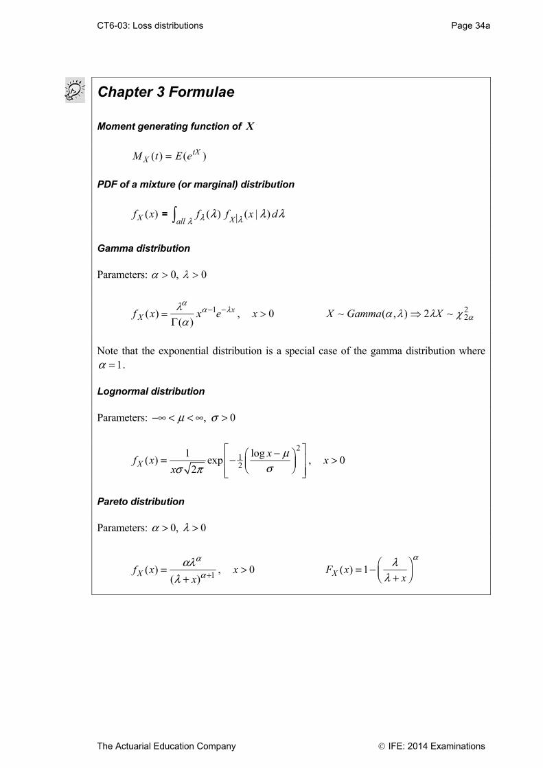
Chapter 3 Formulae Moment generating function of X
M t E eXtX( ) ( )
PDF of a mixture (or marginal) distribution
( )Xf x = ( ) ( | )Xall
f f x dl lll l lΩÚ
Gamma distribution Parameters: 0 0,
f x x eXx( )
( )
1 , x 0 X Gamma X~ ( , ) ~ 2 2
2
Note that the exponential distribution is a special case of the gamma distribution where
1a = . Lognormal distribution Parameters: , 0m s-• < < • >
2
12
1 log( ) exp
2X
xf x
x
mss p
È ˘-Ê ˆ= -Í ˙Á ˜Ë ¯Í ˙Î ˚, 0x >
Pareto distribution Parameters: 0, 0a l> >
1( )
( )Xf x
x
a
aal
l +=+
, 0x > ( ) 1XF xx
all
Ê ˆ= - Á ˜Ë ¯+
Page 34b CT6-03: Loss distributions
IFE: 2014 Examinations The Actuarial Education Company
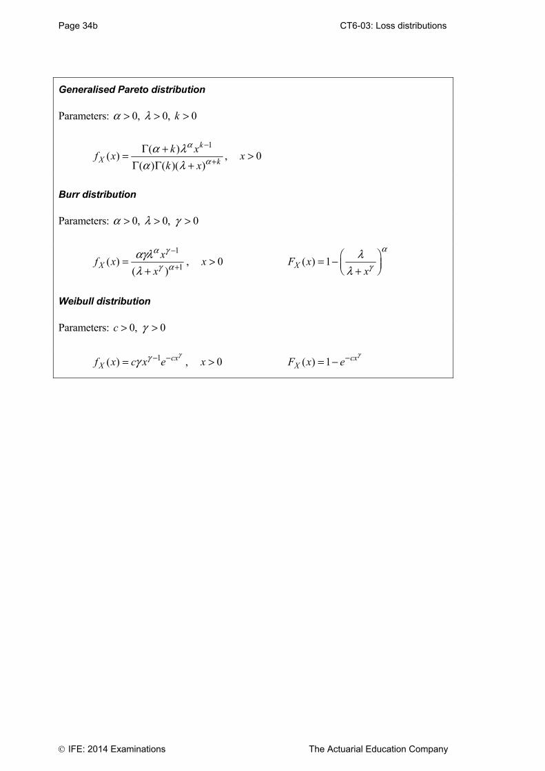
Generalised Pareto distribution Parameters: 0, 0, 0ka l> > >
1( )
( )( ) ( )( )
k
X k
k xf x
k x
a
aa l
a l
-
+G +=
G G +, 0x >
Burr distribution Parameters: 0, 0, 0a l g> > >
1
1( )
( )X
xf x
x
a g
g aagll
-
+=+
, 0x > ( ) 1XF xx
a
gl
lÊ ˆ= - Á ˜Ë ¯+
Weibull distribution Parameters: 0, 0c g> >
1( ) cx
Xf x c x eggg - -= , 0x > ( ) 1 cx
XF x eg-= -

CT6-04: Reinsurance Page 5
The Actuarial Education Company IFE: 2014 Examinations
So the graph looks like this:
We are now in a position to consider the statistical calculations relating to reinsurance arrangements.
1.1 Excess of loss reinsurance
In excess of loss reinsurance, the insurer will pay any claim in full up to an amount M, the retention level; any amount above M will be borne by the reinsurer. In this section “the company” refers to the direct writer. The excess of loss reinsurance arrangement can be written in the following way: if the claim is for amount X then the insurer will pay Y where: Y = X if X M Y = M if X M . The reinsurer pays the amount Z X Y .
Question 4.1
Write down an expression for Y if only a layer between M and 2 M is reinsured.
Page 6 CT6-04: Reinsurance
IFE: 2014 Examinations The Actuarial Education Company
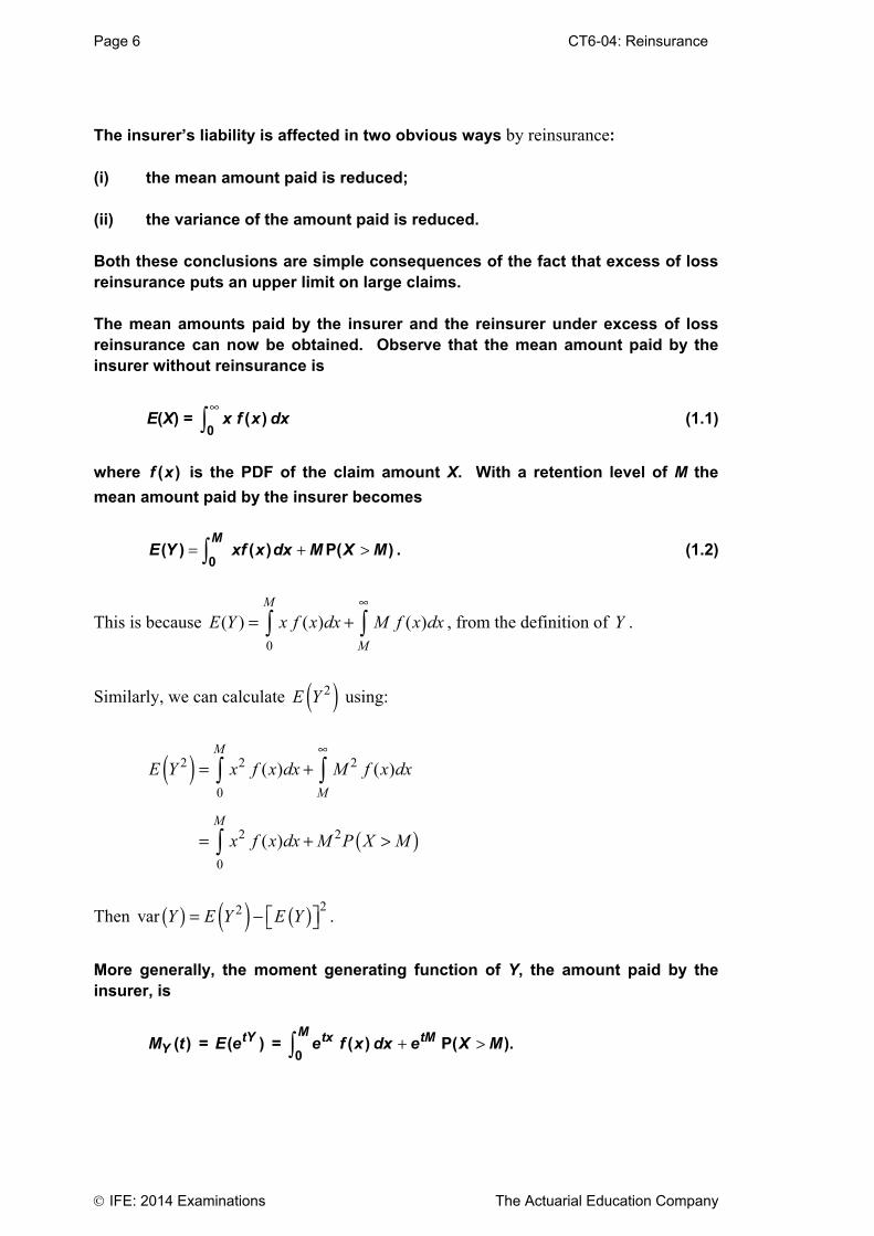
The insurer’s liability is affected in two obvious ways by reinsurance: (i) the mean amount paid is reduced; (ii) the variance of the amount paid is reduced. Both these conclusions are simple consequences of the fact that excess of loss reinsurance puts an upper limit on large claims. The mean amounts paid by the insurer and the reinsurer under excess of loss reinsurance can now be obtained. Observe that the mean amount paid by the insurer without reinsurance is
E(X) = •Ú0 ( )x f x dx (1.1)
where ( )f x is the PDF of the claim amount X. With a retention level of M the
mean amount paid by the insurer becomes
= + >Ú0( ) ( ) P( )M
E Y xf x dx M X M . (1.2)
This is because 0
( ) ( ) ( )M
M
E Y x f x dx M f x dx•
= +Ú Ú , from the definition of Y .
Similarly, we can calculate ( )2E Y using:
( )
( )
2 2 2
0
2 2
0
( ) ( )
( )
M
M
M
E Y x f x dx M f x dx
x f x dx M P X M
•
= +
= + >
Ú Ú
Ú
Then ( ) ( ) ( ) 22var Y E Y E YÈ ˘= - Î ˚ .
More generally, the moment generating function of Y, the amount paid by the insurer, is
( )YM t = ( )tYE e = + >Ú0 ( ) P( ).M tx tMe f x dx e X M

CT6-04: Reinsurance Page 7
The Actuarial Education Company IFE: 2014 Examinations
Question 4.2
Find ( )E Y when X has a Pareto distribution with parameters 200 and 6, and
M 80 .
Under excess of loss reinsurance, the reinsurer will pay Z where: Z = 0 if X M£ Z = X–M if X M> . With a retention level of M the mean amount paid by the reinsurer becomes:
( )( ) ( )M
E Z x M f x dx•
= -Ú , from the definition of Z (1.3)
Similarly, we can calculate ( )2E Z using:
( ) ( )22 ( )M
E Z x M f x dx•
= -Ú
Then ( ) ( ) ( ) 22var Z E Z E ZÈ ˘= - Î ˚ .
More generally, the moment generating function of Z , the amount paid by the reinsurer, is:
( ) ( ) ( )0
0( ) ( )
M t x MtZ tZ M
M t E e e f x dx e f x dx• -= = +Ú Ú
Page 8 CT6-04: Reinsurance
IFE: 2014 Examinations The Actuarial Education Company
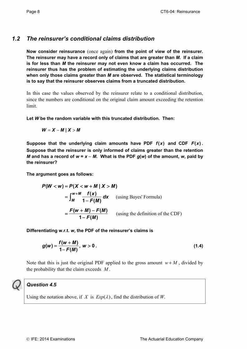
1.2 The reinsurer’s conditional claims distribution
Now consider reinsurance (once again) from the point of view of the reinsurer. The reinsurer may have a record only of claims that are greater than M. If a claim is for less than M the reinsurer may not even know a claim has occurred. The reinsurer thus has the problem of estimating the underlying claims distribution when only those claims greater than M are observed. The statistical terminology is to say that the reinsurer observes claims from a truncated distribution. In this case the values observed by the reinsurer relate to a conditional distribution, since the numbers are conditional on the original claim amount exceeding the retention limit. Let W be the random variable with this truncated distribution. Then: = - >|W X M X M
Suppose that the underlying claim amounts have PDF f x( ) and CDF F x( ) .
Suppose that the reinsurer is only informed of claims greater than the retention M and has a record of w = x M. What is the PDF g(w) of the amount, w, paid by the reinsurer? The argument goes as follows:
(using Bayes' Formula)
(using the definition of the CDF)
( ) ( | )
( )
1 ( )
( ) ( )
1 ( )
w M
M
P W w P X w M X M
f xdx
F M
F w M F M
F M
+
< = < + >
=-
+ -=-
Ú
Differentiating w.r.t. w, the PDF of the reinsurer’s claims is
( )
( )1 ( )
f w Mg w
F M
+=-
, 0w > . (1.4)
Note that this is just the original PDF applied to the gross amount w M+ , divided by the probability that the claim exceeds M .
Question 4.5
Using the notation above, if X is Exp( ) , find the distribution of W.
CT6-04: Reinsurance Page 9
The Actuarial Education Company IFE: 2014 Examinations
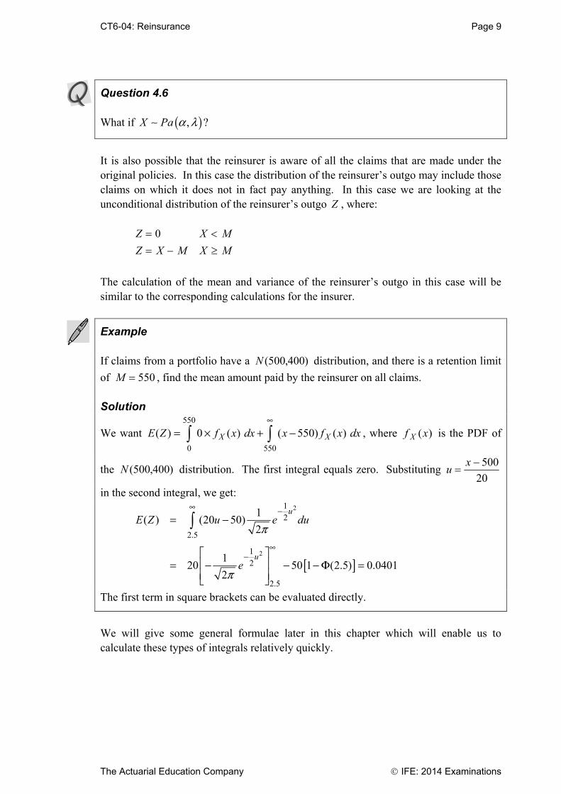
Question 4.6
What if ( ),X Pa a l ?
It is also possible that the reinsurer is aware of all the claims that are made under the original policies. In this case the distribution of the reinsurer’s outgo may include those claims on which it does not in fact pay anything. In this case we are looking at the unconditional distribution of the reinsurer’s outgo Z , where:
Z X M
Z X M X M
0
The calculation of the mean and variance of the reinsurer’s outgo in this case will be similar to the corresponding calculations for the insurer.
Example If claims from a portfolio have a N ( , )500 400 distribution, and there is a retention limit
of M 550 , find the mean amount paid by the reinsurer on all claims. Solution
We want 550
0 550
( ) 0 ( ) ( 550) ( )X XE Z f x dx x f x dx•
= ¥ + -Ú Ú , where f xX ( ) is the PDF of
the N ( , )500 400 distribution. The first integral equals zero. Substituting ux
500
20
in the second integral, we get:
[ ]
2
2
1
2
2.5
1
2
2.5
1( ) (20 50)
2
120 50 1 (2.5) 0.0401
2
u
u
E Z u e du
e
p
p
• -
•-
= -
È ˘Í ˙= - - -F =Í ˙Î ˚
Ú
The first term in square brackets can be evaluated directly.
We will give some general formulae later in this chapter which will enable us to calculate these types of integrals relatively quickly.

Page 10 CT6-04: Reinsurance
IFE: 2014 Examinations The Actuarial Education Company
If we now use W to denote the amount payable by the reinsurer on claims in which it is involved, ie W Z Z X M X M | |0 , then:
E WE Z
P Z
E Z
P X M( )
( )
( )
( )
( )
0
This follows from equation (1.4).
1.3 Proportional reinsurance
In proportional reinsurance the insurer pays a fixed proportion of the claim, whatever the size of the claim. Using the same notation as above, the proportional reinsurance arrangement can be written as follows: if the claim is for an amount X then the company will pay Y where Y X 0 1 . The parameter is known as the retained proportion or retention level; note that the term retention level is used in both excess of loss and proportional reinsurance though it means different things. As the amount paid by the insurer on a claim X is =Y Xa and the amount paid
by the reinsurer is ( )= -1Z Xa , the distribution of both of these amounts can be
found by a simple change of variable.
Question 4.7
Claims occur as a generalised Pareto distribution with parameters 6, 200 and k 4 . A proportional reinsurance arrangement is in force with a retained proportion of 80%. Find the mean and variance of the amount paid by the insurer and the reinsurer on an individual claim.

CT6-04: Reinsurance Page 23
The Actuarial Education Company IFE: 2014 Examinations
And for Year 2:
6
21210 1210 1710
( ) 199.075 1710 5
E YÊ ˆ= - ¥ =Á ˜Ë ¯
So the percentage increase from Year 0 to Year 1 is 7.2%, and the percentage increase from Year 1 to Year 2 is 6.9%.
Note that these figures are less than 10%, as expected.
Question 4.15
What is the limit of ( )nE Y as n tends to infinity?
Page 24 CT6-04: Reinsurance
IFE: 2014 Examinations The Actuarial Education Company
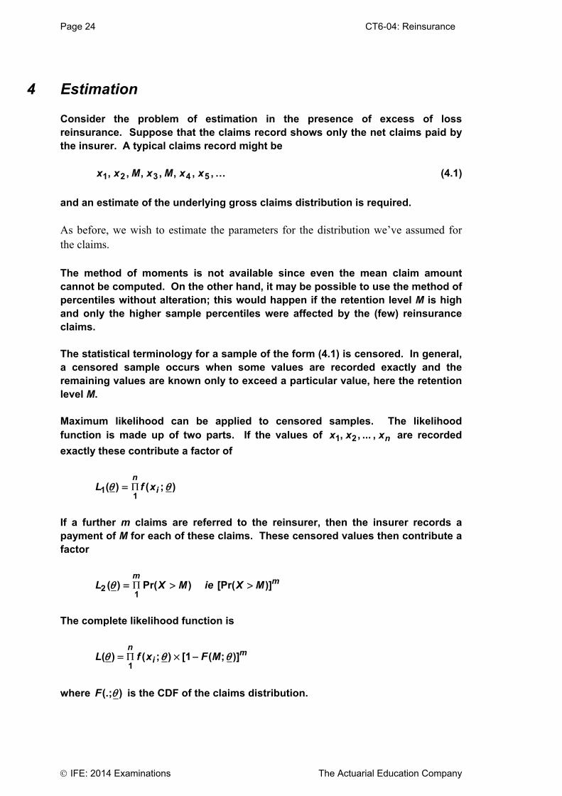
4 Estimation
Consider the problem of estimation in the presence of excess of loss reinsurance. Suppose that the claims record shows only the net claims paid by the insurer. A typical claims record might be x x M x M x x1 2 3 4 5, , , , , , , ... (4.1)
and an estimate of the underlying gross claims distribution is required. As before, we wish to estimate the parameters for the distribution we’ve assumed for the claims. The method of moments is not available since even the mean claim amount cannot be computed. On the other hand, it may be possible to use the method of percentiles without alteration; this would happen if the retention level M is high and only the higher sample percentiles were affected by the (few) reinsurance claims. The statistical terminology for a sample of the form (4.1) is censored. In general, a censored sample occurs when some values are recorded exactly and the remaining values are known only to exceed a particular value, here the retention level M. Maximum likelihood can be applied to censored samples. The likelihood function is made up of two parts. If the values of 1 2, , ... , nx x x are recorded
exactly these contribute a factor of
11
( ) ( ; )n
iL f xq qP=
If a further m claims are referred to the reinsurer, then the insurer records a payment of M for each of these claims. These censored values then contribute a factor
21
( ) Pr( )m
L X Mq P= > ie [Pr( )]mX M>
The complete likelihood function is
P1
( ) ( ; ) [1 ( ; )]n
miL f x F Mq q q= ¥ -
where F(.; ) is the CDF of the claims distribution.
CT6-04: Reinsurance Page 31
The Actuarial Education Company IFE: 2014 Examinations
Chapter 4 Summary Reinsurance Reinsurance is insurance for insurance companies. By using reinsurance, the insurer seeks to protect itself from large claims. The mean amount paid by the insurer is reduced, and the variance of the amount paid by the insurer is reduced. Reinsurance may be proportional or non-proportional (ie individual excess of loss). Proportional reinsurance Under proportional reinsurance, the insurer and the reinsurer split the claim in pre-defined proportions. For a claim amount X , the amount paid by the insurer is Y Xa= and the
amount paid by the reinsurer is ( )1Z Xa= - where a is known as the retained
proportion or retention level, 0 1a< < . Non-proportional reinsurance (individual excess of loss) Under individual excess of loss, the insurer will pay any claim in full up to an amount M , the retention level; any amount above M will be met by the reinsurer. For a claim amount, X , the amount paid by the insurer is:
X if X M
YM if X M
£Ï= Ì >Ó
The amount paid by the reinsurer is:
0 if X M
ZX M if X M
£Ï= Ì - >Ó

Page 32 CT6-04: Reinsurance
IFE: 2014 Examinations The Actuarial Education Company
Reinsurer’s conditional claims distribution It may be the case that the reinsurer is only informed of claims greater than the retention level M . In this case, the reinsurer observes claims from a truncated (or conditional) distribution. Let W be the random variable associated with this distribution, then: | 0 |W Z Z X M X M= > = - >
The PDF of the reinsurer’s conditional distribution is given by:
( )
( )1 ( )
XW
X
f w Mg w
F M
+=-
Excesses When a policy excess applies, the policyholder pays for the first part of each loss up to an excess level L ; any amount greater than L will be met by the insurer. The positions of the policyholder and the insurer as far as losses are concerned are the same as those of the insurer and the reinsurer respectively under individual excess of loss reinsurance. When a policy excess applies, the insurer’s conditional distribution takes the same form as that of the reinsurer’s conditional distribution above. Inflation and individual excess of loss reinsurance If claims are inflated by a factor of k but the retention level remains fixed at M then the amount paid by the insurer is:
kX if kX M
YM if kX M
£Ï= Ì >Ó
The amount paid by the reinsurer is:
0 if kX M
ZkX M if kX M
£Ï= Ì - >Ó
CT6-04: Reinsurance Page 33
The Actuarial Education Company IFE: 2014 Examinations
Chapter 4 Formulae Claim amounts paid by insurer and reinsurer
Suppose that X is the amount of an original claim having PDF ( )Xf x , Y is the amount
paid by the insurer and Z X Y= - is the amount paid by the reinsurer. Under a proportional reinsurance treaty with a retained proportion of :
[ ]
2
3
3
3/ 2 3/ 22
( ) ( )
var( ) var( )
skew( ) skew( )
skew( ) skew( )( ) ( )
var( ) var( )
E Y E X
Y X
Y X
Y XCoeff of skew Y Coeff of skew X
Y X
a
a
a
a
a
=
=
=
= = =È ˘Î ˚
Under an individual excess of loss treaty with a retention level of M :
X if X M
YM if X M
£Ï= Ì >Ó
and 0 if X M
ZX M if X M
£Ï= Ì - >Ó
We have:
( )0
0
( ) ( ) ( )
( ) 1
MX XM
MX
E Y x f x dx M f x dx
x f x dx M F M
•= +
È ˘= + -Î ˚
Ú ÚÚ
( ) ( )2 2 2
0( ) 1
MXE Y x f x dx M F MÈ ˘= + -Î ˚Ú
( ) ( ) ( ) 22var Y E Y E YÈ ˘= - Î ˚
( ) ( ) ( )0
( ) 1MtY tx tM
Y XM t E e e f x dx e F MÈ ˘= = + -Î ˚Ú
Page 34 CT6-04: Reinsurance
IFE: 2014 Examinations The Actuarial Education Company
And:
( )( ) ( )XME Z x M f x dx
•= -Ú
( ) ( )22 ( )XME Z x M f x dx
•= -Ú
( ) ( ) ( ) 22var Z E Z E ZÈ ˘= - Î ˚
( ) ( ) ( )0
( ) ( )M t x MtZ
Z X XMM t E e f x dx e f x dx
• -= = +Ú Ú
Note that ( ) ( ) ( )E X E Y E Z= + but var( ) var( ) var( )X Y Zπ + since Y and Z are not
independent. If X takes a lognormal or normal distribution, the following results will help with the integration: Lognormal distribution
2 2½( ) [ ( ) ( )]U
k k kX k k
L
x f x dx e U Lm s+= F -FÚ
where log
kL
L km s
s-= - and
logk
UU k
m ss-= -
( ) 0F -• = (0) ½F = ( ) 1F • =
Normal distribution
( ) [ ( ) ( )] [ ( ) ( )]U
XL
x f x dx U L U Lm s f f= F -F - -¢ ¢ ¢ ¢Ú
where
LL
and
UU
( ) ( ) 0
CT6-04: Reinsurance Page 34a
The Actuarial Education Company IFE: 2014 Examinations
Distribution of reinsurer’s claim amounts on claims in which it is involved Let |W X M X M= - > , so that W represents the amount paid by the reinsurer given
that the reinsurer is involved in the claim. Then the PDF of W is:
( )( )
1 ( )X
WX
f w Mg w
F M
+=-
and: ( )
( )( 0)
E ZE W
P Z=
> where:
0 if
if
X MZ
X M X M
£Ï= Ì - >Ó
Using the PDF above of W it can be shown that: 1. if ~ ( )X Exp l , then |X M X M- > is ( )Exp l
2. if ~ ( , )X Pareto a l , then |X M X M- > is ( , )Pareto Ma l + .
Estimation of parameters from a censored sample
The likelihood function of a vector of parameters q , based on a sample of n exact
observations and m censored observations known to exceed M is:
[ ]1
( ) ( ) ( )n
mX i
i
L f x P X Mq=
È ˘= >Í ˙Í ˙Î ˚’
assuming that the observations are realisations of n m+ IID random variables.

Page 34b CT6-04: Reinsurance
IFE: 2014 Examinations The Actuarial Education Company
This page has been left blank so that you can keep the chapter summaries
together as a revision tool.

CT6-05: Credibility theory Page 27
The Actuarial Education Company IFE: 2014 Examinations
Chapter 5 Summary Direct vs collateral data Claim numbers or aggregate claim amounts can be estimated using a combination of direct data (ie data from the risk under consideration) and collateral data (ie data from other similar, but not necessarily identical, risks). Credibility premium and credibility factor
Let X be an estimate of the expected number of claims/aggregate claim amount for a particular risk for the coming year based on direct data. Let m be an estimate of the expected number of claims/aggregate claims for a particular
risk for the coming year based on collateral data. The credibility premium (or credibility estimate of the number of claims/aggregate claim amount) for this risk is:
( )1CP ZX Z m= + -
where Z is a number between 0 and 1 and is known as the credibility factor. The closer it is to 1, the more weight is given to the direct data. The problem remains as to how to calculate Z . There are two approaches: Bayesian credibility and empirical Bayes credibility theory (EBCT). Bayesian credibility The problem of interest is to estimate a parameter (for example a parameter representing the mean number of claims or mean claim amount) and then to express the estimator as a credibility premium. Following the approach developed in Chapter 2, we combine the prior PDF and the likelihood of the sample data using Bayes’ formula to obtain the posterior PDF. A Bayesian estimator of the parameter is obtained to minimise the expected value of some loss function.

Page 28 CT6-05: Credibility theory
IFE: 2014 Examinations The Actuarial Education Company
The Bayesian estimator is then shown to be in the form of a credibility premium:
Bayesian estimator = ( )1CP ZX Z m= + -
where X is the MLE of the parameter based on the sample data and m is an estimator
based on the prior distribution. Z is the credibility factor, a number between 0 and 1 that shows how much weight the Bayesian estimator places on the sample data and how much on the prior distribution. Example formulae are given for the following three models (combinations of likelihood and prior) on the next page:
1. Poisson/gamma model
2. Normal/normal model
3. Binomial/beta model.
CT6-05: Credibility theory Page 28a
The Actuarial Education Company IFE: 2014 Examinations
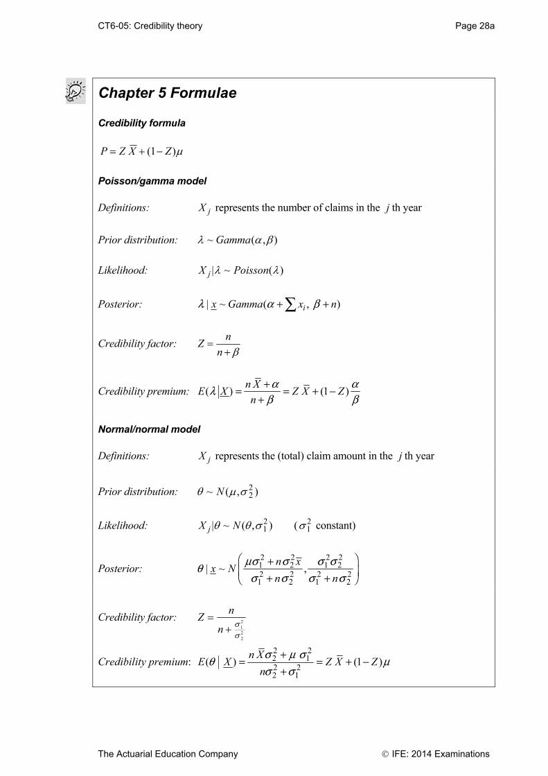
Chapter 5 Formulae Credibility formula
P Z X Z ( )1
Poisson/gamma model Definitions: X j represents the number of claims in the j th year
Prior distribution: ~ ( , )Gamma
Likelihood: X Poissonj | ~ ( )
Posterior: | ~ ( , )ix Gamma x nl a b+ +Â
Credibility factor: Zn
n
Credibility premium: ( ) (1 )n X
E X Z X Zn
a alb b+= = + -+
Normal/normal model
Definitions: X j represents the (total) claim amount in the j th year
Prior distribution: ~ ( , )N 22
Likelihood: X Nj | ~ ( , ) 12 (1
2 constant)
Posterior: 2 2 2 21 2 1 22 2 2 21 2 1 2
| ~ ,n x
x Nn n
ms s s sqs s s s
Ê ˆ+Á ˜+ +Ë ¯
Credibility factor: Zn
n
12
22
Credibility premium: 2 22 12 22 1
( ) (1 )n X
E X Z X Zn
s m sq ms s
+= = + -+
Page 28b CT6-05: Credibility theory
IFE: 2014 Examinations The Actuarial Education Company
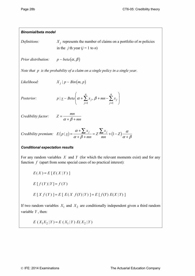
Binomial/beta model Definitions: X j represents the number of claims on a portfolio of m policies
in the j th year (j = 1 to n)
Prior distribution: ( ),p beta a b
Note that p is the probability of a claim on a single policy in a single year.
Likelihood: ( )| ,jX p Bin m p
Posterior: 1 1
| ,n n
j jj j
p x Beta x mn xa b= =
Ê ˆ+ + -Á ˜
Ë ¯Â Â
Credibility factor: mn
Zmna b
=+ +
Credibility premium: ( ) ( )| 1j jx x
E p x Z Zmn mn
a aa b a b
+= = + -
+ + +Â Â
Conditional expectation results For any random variables X and Y (for which the relevant moments exist) and for any function f (apart from some special cases of no practical interest):
( ) [ ( | ) ]E X E E X Y=
[ ( ) | ] ( )E f Y Y f Y=
[ ( ) ] [ ( ( ) | ) ] [ ( ) ( | ) ]E X f Y E E X f Y Y E f Y E X Y= =
If two random variables 1X and 2X are conditionally independent given a third random
variable Y , then: 1 2 1 2( | ) ( | ) ( | )E X X Y E X Y E X Y=

CT6-06: Empirical Bayes Credibility theory Page 41
The Actuarial Education Company © IFE: 2014 Examinations
Chapter 6 Summary Empirical Bayes credibility This approach to credibility theory assumes that the number of claims or aggregate claim amount for each risk are dependent on an underlying risk parameter . However, no assumptions are made about the form of the distribution of q . The credibility premium can be expressed in terms of a credibility factor, which depends on the mean and variance of the conditional claim distribution. These quantities can be estimated based on data derived from a number of different risks. Empirical Bayes Credibility Theory Model 1 Definitions: ijX represents the number of claims (or aggregate claim amount)
for risk ( 1... )i i n= in year ( 1... )j j N= .
Assumptions: For each risk i , the distribution of ijX depends on a parameter iq
whose value is the same for each j but is unknown.
|ij iX q are i.i.d random variables.
iq are i.i.d random variables.
For i kπ , the pairs ( ),ij iX q and ( ),km kX q are i.i.d random
variables.
There exist functions ( )m and ( )2s such that:
( ) ( )2( ) | ( ) var |i ij i ijm E X s Xq q q q= = .
Estimators: Unbiased estimators for ( )E m qÈ ˘Î ˚ , ( )2E s qÈ ˘Î ˚ and ( )var m qÈ ˘Î ˚ are
given on Page 29 of the Tables.
Credibility factor:
[ ]2( )
var ( )
nZ
E sn
m
=Ê ˆÈ ˘
Î ˚Á ˜+Á ˜Ë ¯
Credibility premium: We are trying to estimate ( )im q given X . The estimator, or
credibility premium is ( )1iZ X Z X+ - .

Page 42 CT6-06: Empirical Bayes Credibility theory
© IFE: 2014 Examinations The Actuarial Education Company
Empirical Bayes Credibility Theory Model 2
Definitions: ijY represents the number of claims (or aggregate claim amount)
for risk ( 1... )i i n= in year ( 1... )j j N= .
ijP represents the corresponding risk volume (eg number of
policies or premium income). The ijP ’s are assumed to be known.
/ij ij ijX Y P=
Assumptions: For each risk i , the distribution of ijX depends on a parameter iq
whose value is the same for each j but is unknown.
|ij iX q are independent random variables.
iq are i.i.d random variables.
For i kπ , the pairs ( ),ij iX q and ( ),km kX q are independent
random variables.
There exist functions ( )m and ( )2s such that:
( ) ( )2( ) | ( ) var |i ij i ij ijm E X s P Xq q q q= =
Estimators: Unbiased estimators for ( )E m qÈ ˘Î ˚ , ( )2E s qÈ ˘Î ˚ and ( )var m qÈ ˘Î ˚ are
given on Page 30 of the Tables.
Credibility factor:
[ ]
1
2
1
( )
var ( )
n
ijj
in
ijj
P
ZE s
Pm
=
=
=Ê ˆÈ ˘
Î ˚Á ˜+Á ˜Ë ¯
Â
Â
Credibility premium: We are trying to estimate ( )im q given X . The estimator, or
credibility premium is ( )1i i iZ X Z X+ - .

CT6-07: Risk models (1) Page 19
The Actuarial Education Company IFE: 2014 Examinations
The next three sections consider compound distributions using various models for the number of claims, N. Of the three types of compound distribution described, the compound Poisson is the one that has been asked about most often in past examination questions. However, they are all important. Note that the compound geometric distribution mentioned in the syllabus item is just a specific example of a compound negative binomial distribution.
3.4 The compound Poisson distribution
First consider aggregate claims when N has a Poisson distribution with mean
denoted ( )N Poi l . S then has a compound Poisson distribution with
parameter , and F x( ) is the CDF of the individual claim amount random
variable. F x( ) here represents a general distribution for the individual claim amounts.
The results required for this distribution for N are:
= =[ ] var[ ]E N N l
M t eNt( ) exp ( ) 1
Note that these results are given in the Tables. Check that you can derive them. These results can be combined with those of Section 3.1 as follows: from (3.3), E S m[ ] 1 (3.8)
from (3.4), = 2var[ ]S ml (3.9)
ie ( )m m m2 12
12

Page 20 CT6-07: Risk models (1)
IFE: 2014 Examinations The Actuarial Education Company
and from (3.7), M t M tS X( ) exp ( ( ) ) 1 (3.10)
The results for the mean and variance have a very simple form. Note that the variance of S is expressed in terms of the second moment of X i about zero (and
not in terms of the variance of X i ).
Note also that the formula for the skewness of S has a simple form when S is a compound Poisson random variable: = 3[ ]skew S ml (3.11)
In order to find the skewness of a compound Poisson distribution, we need to use cumulant generating functions (CGFs). These were covered in Subject CT3, but we provide the theory required again here. The cumulant generating function ( )XC t is defined by:
( ) log ( )X XC t M t=
Mean, variance and skewness in terms of ( )C tX
CGF Results If the cumulant generating function of a random variable X is ( )XC t , then:
( ) (0)XE X C= ¢ var( ) (0)XX C= ¢¢ skew( ) (0)XX C= ¢¢¢
The CGF of X is: ( ) log ( )X XC t M t=
Differentiating this using the chain rule (or function-of-a-function rule):
1 ( )( ) ( )
( ) ( )X
X XX X
M tC t M t
M t M t
¢= ¥ =¢ ¢
Putting t 0 :
(0) ( )(0) ( )
(0) 1X
XX
M E XC E X
M
¢= = =¢

CT6-07: Risk models (1) Page 21
The Actuarial Education Company IFE: 2014 Examinations
Differentiating again, using the product rule and the chain rule:
2
2 2
1 ( ) ( ) [ ( )]( ) ( ) ( )
( ) ( )[ ( )] [ ( )]X X X
X X XX XX X
M t M t M tC t M t M t
M t M tM t M t
- ¢ ¢¢ ¢= ¥ + ¥ = -¢¢ ¢¢ ¢
Putting t 0 :
22 2
2
(0) [ (0)](0) ( ) [ ( )] var( )
(0) [ (0)]X X
XX X
M MC E X E X X
M M
¢¢ ¢= - = - =¢¢
Differentiating again, and simplifying, gives:
3
2 3
( ) ( ) ( ) [ ( )]( ) 3 2
( ) [ ( )] [ ( )]X X X X
XX X X
M t M t M t M tC t
M t M t M t
¢¢¢ ¢¢ ¢ ¢= - +¢¢¢
Putting t 0 :
3
2 3
3 2 3
(0) (0) (0) [ (0)](0) 3 2
(0) [ (0)] [ (0)]
( ) 3 ( ) ( ) 2[ ( )] skew( )
X X X XX
X X X
M M M MC
M M M
E X E X E X E X X
¢¢¢ ¢¢ ¢ ¢= - +¢¢¢
= - + =
Using these results, we can show that the skewness of the compound Poisson distribution is m3 .
An alternative approach would be to expand log ( )t XE e as a power series and look at the
coefficients of individual terms. The easiest way to show that the third central moment of S is m3 is to use the cumulant generating function: =( ) log ( )S SC t M t
To determine the skewness, we differentiate it three times with respect to t and set = 0t , ie:
E S md
dtM tS t[( ) ] log ( )| 1
33
3 0

Page 22 CT6-07: Risk models (1)
IFE: 2014 Examinations The Actuarial Education Company
Now ( )log ( ) ( ) 1S XM t M tl= - , so:
0
3 3
33 3log ( ) ( ) 1
t
S Xd d
M t M t mdt dt
l l=
È ˘= - =Í ˙
Í ˙Î ˚
This is because 3(0) ( )XM E X=¢¢¢ for any random variable.
ie E S m m[( ) ] 13
3
and the coefficient of skewness = m m3 23 2/ ( ) / .
For the compound Poisson it is worth remembering the formulae m1 , m2 and m3
for the mean, variance and skewness. However, they are given in the Tables. This result shows that the distribution of S is positively skewed, since m3 is the
third moment about zero of Xi and hence is greater than zero because Xi is a
non-negative valued random variable. Note that the distribution of S is positively skewed even if the distribution of Xi is negatively skewed. The coefficient of
skewness of S is m m3 23 2/ ( ) / , and hence goes to 0 as . Thus for large
values of , the distribution of S is almost symmetric.
Sums of compound Poisson distributions A very useful property of the compound Poisson distribution is that the sum of independent compound Poisson random variables is itself a compound Poisson random variable. A formal statement of this property is as follows. Let S1, S2, ..., Sn be independent random variables. Suppose that each Si has a
compound Poisson distribution with parameter i , and that the CDF of the
individual claim amount random variable for each iS is F xi ( ) .
Define A = S1 + S2 + + Sn. Then A has a compound Poisson distribution with
parameter , and F x( ) is the CDF of the individual claim amount random
variable for A , where:
ii
n
1
and F x F xi ii
n
( ) ( )1
1
is just the capital form of the Greek letter .
CT6-07: Risk models (1) Page 23
The Actuarial Education Company IFE: 2014 Examinations
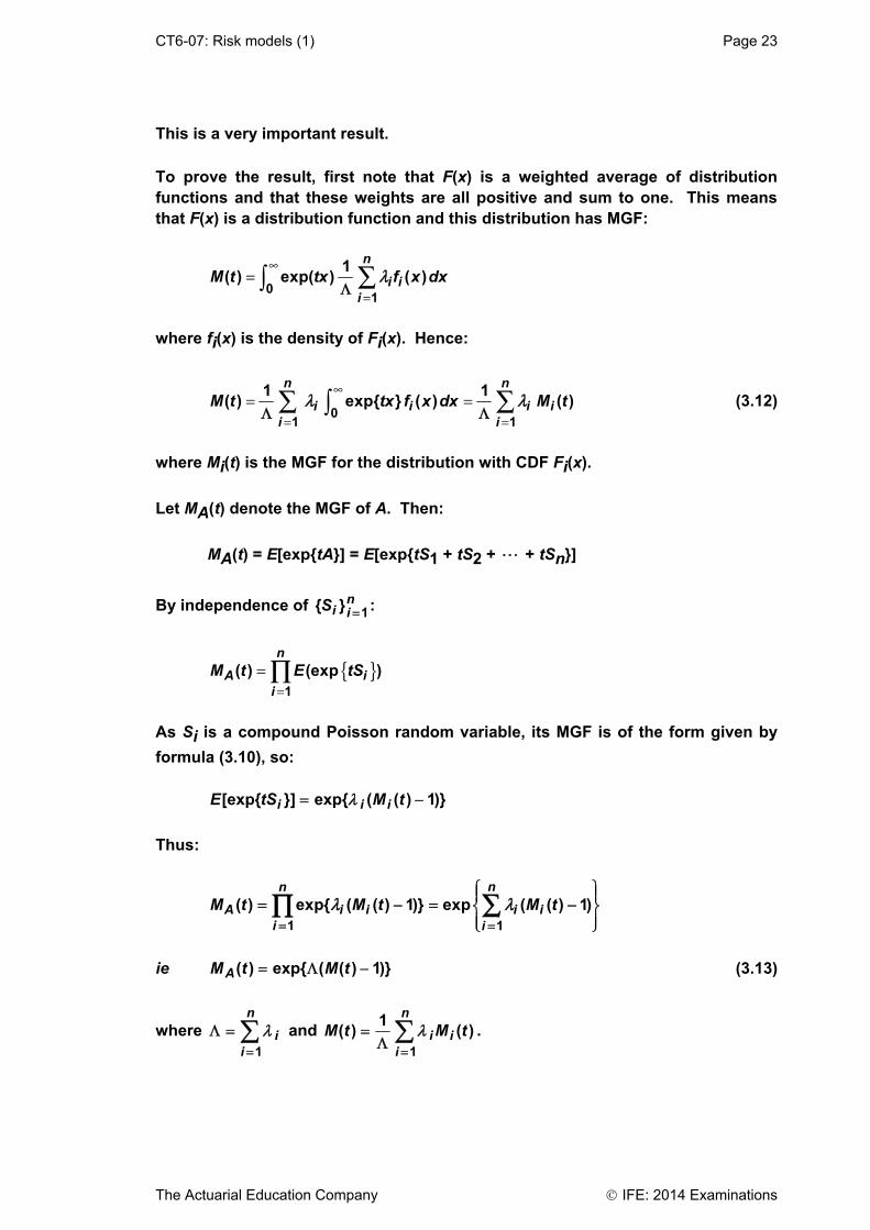
This is a very important result. To prove the result, first note that F(x) is a weighted average of distribution functions and that these weights are all positive and sum to one. This means that F(x) is a distribution function and this distribution has MGF:
•
== ÂÚ0
1
1( ) exp( ) ( )
n
i ii
M t tx f x dxlL
where fi(x) is the density of Fi(x). Hence:
•
= == =Â ÂÚ0
1 1
1 1( ) exp ( ) ( )
n n
i i i ii i
M t tx f x dx M tl lL L
(3.12)
where Mi(t) is the MGF for the distribution with CDF Fi(x).
Let MA(t) denote the MGF of A. Then:
MA(t) = E[exptA] = E[exptS1 + tS2 + + tSn]
By independence of Si in1:
=
=’1
( ) (exp )n
A ii
M t E tS
As Si is a compound Poisson random variable, its MGF is of the form given by
formula (3.10), so:
E tS M ti i i[exp ] exp ( ( ) ) 1
Thus:
1 1
( ) exp ( ( ) 1) exp ( ( ) 1)nn
A i i i ii i
M t M t M tl l= =
Ï ¸Ô Ô= - = -Ì ˝Ô ÔÓ ˛Â’
ie M t M tA( ) exp ( ( ) ) 1 (3.13)
where ii
n
1
and M t M ti ii
n
( ) ( )1
1
.

Page 24 CT6-07: Risk models (1)
IFE: 2014 Examinations The Actuarial Education Company
By the one-to-one relationship between distributions and MGFs, formula (3.13) shows that A has a compound Poisson distribution with Poisson parameter . By (3.12), the individual claim amount distribution has CDF F(x).
Question 7.8
The distributions of aggregate claims from two risks, denoted by S1 and S2 , are as
follows: S1 has a compound Poisson distribution with parameter 100 and distribution
function F x x1 1( ) exp( / ) , x 0 and S2 has a compound Poisson distribution
with parameter 200 and distribution function F x x x2 1 0( ) exp( / ), . If S1 and
S2 are independent, what is the distribution of S S1 2 ?
3.5 The compound binomial distribution
Under certain circumstances, the binomial distribution is a natural choice for N. For example, under a group life insurance policy covering n lives, the distribution of the number of deaths in a year is binomial if it is assumed that each insured life is subject to the same mortality rate, and that lives are independent with respect to mortality. The notation N ~ bin(n, p) is used to denote the binomial distribution for N. The key results for this distribution are:
E[N] = np
var[N] = np(1 p)
MN (t) = (pet + 1 p)n
Note that these results are given in the Tables. However, the notation for the MGF is slightly different. Again, check that you can derive the results for yourself. When N has a binomial distribution, S has a compound binomial distribution. One important point about choosing the binomial distribution for N is that there is an upper limit, n, to the number of claims. Expressions for the mean, variance and MGF of S are now found in terms of n, p, m1, m2 and MX (t) when N ~ bin(n, p).
CT6-07: Risk models (1) Page 25
The Actuarial Education Company IFE: 2014 Examinations
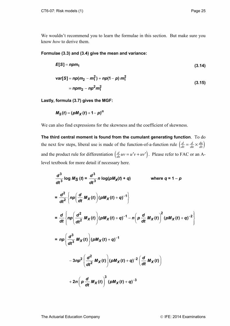
We wouldn’t recommend you to learn the formulae in this section. But make sure you know how to derive them. Formulae (3.3) and (3.4) give the mean and variance: = 1[ ]E S npm (3.14)
= - + -
= -
2 22 1 1
2 22 1
var[ ] ( ) (1 )S np m m np p m
npm np m (3.15)
Lastly, formula (3.7) gives the MGF:
= + -( ) ( ( ) 1 )nS XM t pM t p
We can also find expressions for the skewness and the coefficient of skewness. The third central moment is found from the cumulant generating function. To do
the next few steps, liberal use is made of the function-of-a-function rule ( )d d dudx du dx= ¥
and the product rule for differentiation ( )ddx uv u v uv= +¢ ¢ . Please refer to FAC or an A-
level textbook for more detail if necessary here.
d
dt
3
3log MS (t) =
d
dt
3
3n log(pMx(t) + q) where q = 1 p
= -Ï ¸Ê ˆ +Ì ˝Á ˜Ë ¯Ó ˛
21
2( ) ( ( ) )X X
d dnp M t pM t q
dtdt
= - -Ï ¸Ê ˆÔ ÔÊ ˆ+ - +Ì ˝Á ˜ Á ˜Ë ¯Ë ¯Ô ÔÓ ˛
221 2
2( ) ( ( ) ) ( ) ( ( ) )X X X X
d d dnp M t pM t q n p M t pM t q
dt dtdt
= -Ê ˆ+Á ˜
Ë ¯
31
3( ) ( ( ) )X X
dnp M t pM t q
dt
-Ê ˆ Ê ˆ- +Á ˜ Á ˜Ë ¯Ë ¯
22 2
23 ( ) ( ( ) ) ( )X X X
d dnp M t pM t q M t
dtdt
-Ê ˆ+ +Á ˜Ë ¯
332 ( ) ( ( ) )X X
dn p M t pM t q
dt

Page 26 CT6-07: Risk models (1)
IFE: 2014 Examinations The Actuarial Education Company
You may find this algebra easier to follow if you write it out for yourself using M x( )
and so on for the derivatives.
We can now find a formula for the skewness of S , which is 3[( ( )) ]E S E S- .
Setting t = 0 gives:
- = - +3 2 3 31 3 2 1 1[( ) ] 3 2E S npm npm np m m np m (3.16)
The coefficient of skewness is then given by
- +-
2 3 33 2 1 1
2 2 3/22 1
3 2
( )
npm np m m np m
npm np m
It can be deduced from formula (3.16) that it is possible for the compound binomial distribution to be negatively skewed. The simplest illustration of this fact is when all claims are of amount B. Here, B is a fixed number. Then S BN=
and:
E[(S E(S))3] = B3 E[(N E[N])3] so that the coefficient of skewness of S is a multiple of that for N. If > 0.5p , then
the binomial distribution for N is negatively skewed.

CT6-07: Risk models (1) Page 33
The Actuarial Education Company IFE: 2014 Examinations
Chapter 7 Summary Insurable risks For a risk to be insurable the policyholder should have an interest in the risk being insured to distinguish between insurance and a wager, and it should be of a financial and reasonably quantifiable nature. Ideally, risk events should:
be independent
have low probability of occurring
be pooled with similar risks
have an ultimate liability
avoid moral hazards. Characteristics of general insurance products Most general insurance contracts share the following characteristics:
Cover is normally for a fixed period, typically a year, after which it needs to be renegotiated.
There is usually no obligation to continue cover although in most cases a need for continuing cover may be assumed to exist.
Claims are not of fixed amounts.
The existence of a claim and its amount have to be proved before a claim can be settled.
A claim occurring does not bring the policy to an end.
Claims that take a long time to settle are known as long-tailed and those that take a short time to settle are known as short-tailed.
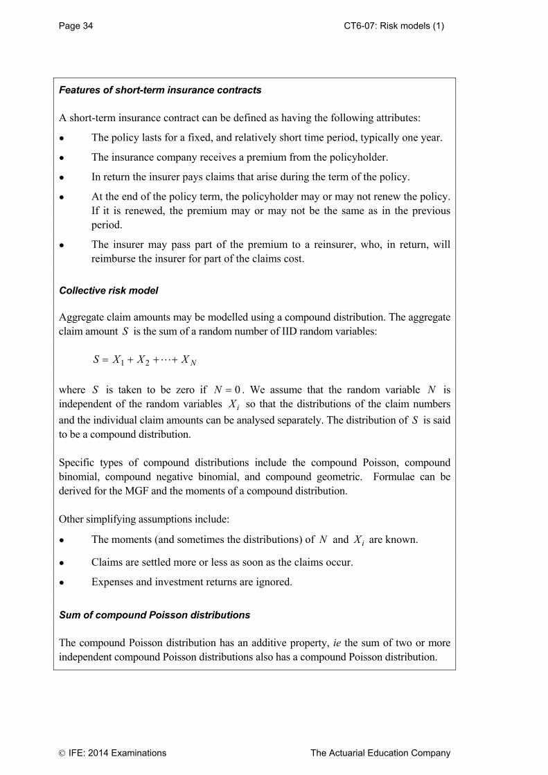
Page 34 CT6-07: Risk models (1)
IFE: 2014 Examinations The Actuarial Education Company
Features of short-term insurance contracts A short-term insurance contract can be defined as having the following attributes:
The policy lasts for a fixed, and relatively short time period, typically one year.
The insurance company receives a premium from the policyholder.
In return the insurer pays claims that arise during the term of the policy.
At the end of the policy term, the policyholder may or may not renew the policy. If it is renewed, the premium may or may not be the same as in the previous period.
The insurer may pass part of the premium to a reinsurer, who, in return, will reimburse the insurer for part of the claims cost.
Collective risk model Aggregate claim amounts may be modelled using a compound distribution. The aggregate claim amount S is the sum of a random number of IID random variables: S X X X N 1 2
where S is taken to be zero if N 0 . We assume that the random variable N is independent of the random variables Xi so that the distributions of the claim numbers
and the individual claim amounts can be analysed separately. The distribution of S is said to be a compound distribution. Specific types of compound distributions include the compound Poisson, compound binomial, compound negative binomial, and compound geometric. Formulae can be derived for the MGF and the moments of a compound distribution. Other simplifying assumptions include:
The moments (and sometimes the distributions) of N and iX are known.
Claims are settled more or less as soon as the claims occur.
Expenses and investment returns are ignored.
Sum of compound Poisson distributions The compound Poisson distribution has an additive property, ie the sum of two or more independent compound Poisson distributions also has a compound Poisson distribution.

CT6-07: Risk models (1) Page 35
The Actuarial Education Company IFE: 2014 Examinations
Chapter 7 Formulae Probability/moment generating function of X
G t E tXX( ) ( ) ( ) ( )tX
XM t E e=
Generating functions of compound distributions G t G G tS N X( ) [ ( )] M t M M tS N X( ) [log ( )]
Mean and variance of compound distributions
( ) ( ) ( )E S E N E X= 2var( ) ( )var( ) var( )[ ( )]S E N X N E X= +
Compound Poisson distribution
1( )E S ml= 2var( )S ml= skew( )S m 3
( ) ( )( ) 1XM tSM t el -=
Compound binomial distribution
1( )E S npm= 2 22 1var( )S npm np m= -
2 3 33 2 1 1skew( ) 3 2S npm np m m np m= - + ( ) ( ) n
S XM t pM t qÈ ˘= +Î ˚
Compound negative binomial distribution
1( )kq
E S mp
= 2
22 12
var( )kq kq
S m mp p
= +
skew( )Skq
pm
kq
pm m
kq
pm 3
2
2 1 2
3
3 133 2
( )( )1
k
S kX
pM t
qM t=È ˘-Î ˚
Cumulant generating function
( ) log ( )X XC t M t=
( ) (0)XE X C= ¢ var( ) (0)XX C= ¢¢ skew( ) (0)XX C= ¢¢¢
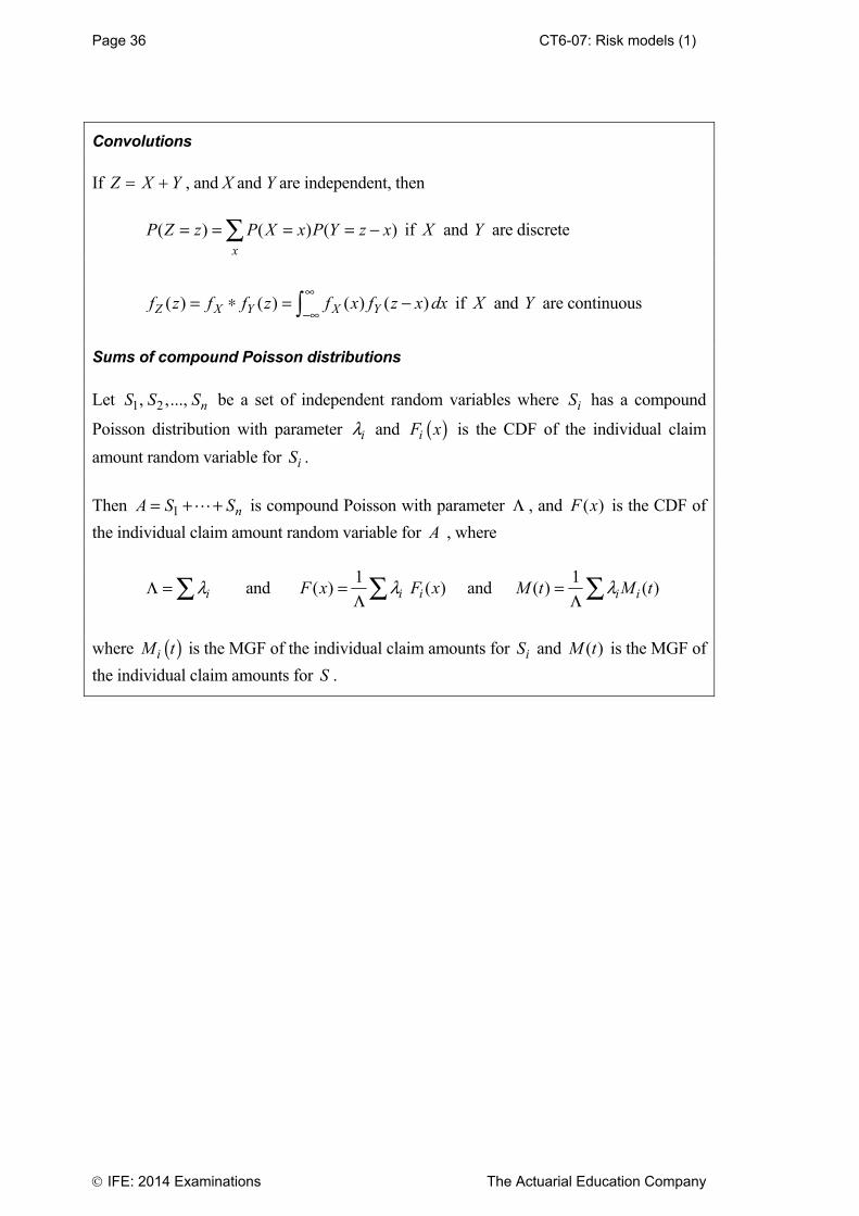
Page 36 CT6-07: Risk models (1)
IFE: 2014 Examinations The Actuarial Education Company
Convolutions If Z X Y , and X and Y are independent, then
( ) ( ) ( )x
P Z z P X x P Y z x= = = = -Â if X and Y are discrete
( ) ( ) ( ) ( )Z X Y X Yf z f f z f x f z x dx•
-•= * = -Ú if X and Y are continuous
Sums of compound Poisson distributions
Let 1 2, ,..., nS S S be a set of independent random variables where iS has a compound
Poisson distribution with parameter il and ( )iF x is the CDF of the individual claim
amount random variable for iS .
Then 1 nA S S= + + is compound Poisson with parameter L , and ( )F x is the CDF of
the individual claim amount random variable for A , where
ilL =Â and 1
( ) ( )i iF x F xl=LÂ and
1( ) ( )i iM t M tl=
LÂ
where ( )iM t is the MGF of the individual claim amounts for iS and ( )M t is the MGF of
the individual claim amounts for S .
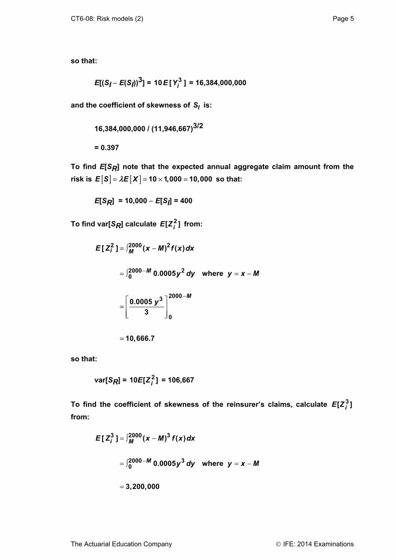
CT6-08: Risk models (2) Page 5
The Actuarial Education Company IFE: 2014 Examinations
so that:
E[(SI E(SI))3] = 310 [ ]iE Y = 16,384,000,000
and the coefficient of skewness of IS is:
16,384,000,000 / (11,946,667)3/2
= 0.397 To find E[SR] note that the expected annual aggregate claim amount from the
risk is [ ] [ ]= = ¥ =10 1,000 10,000E S E Xl so that:
E[SR] = 10,000 E[SI] = 400
To find var[SR] calculate E Zi[ ]2 from:
-
-
= Ú -
= Ú = -
È ˘= Í ˙Í ˙Î ˚
=
2 2000 2
2000 20
20003
0
[ ] ( ) ( )
0.0005 where
0.0005
3
10,666.7
i M
M
M
E Z x M f x dx
y dy y x M
y
so that:
var[SR] = 10 2E Zi[ ] = 106,667
To find the coefficient of skewness of the reinsurer’s claims, calculate E Zi[ ]3
from:
-
= Ú -
= Ú = -
=
3 2000 3
2000 30
[ ] ( ) ( )
0.0005 where
3,200,000
i M
M
E Z x M f x dx
y dy y x M

Page 6 CT6-08: Risk models (2)
IFE: 2014 Examinations The Actuarial Education Company
so that:
3 3[ ( [ ]) ] 10 [ ] 32,000,000R R iE S E S E Z- = =
and the coefficient of skewness of RS is:
3 / 232,000,000 /(106,667) 0.92
Question 8.2
What is the variance of S , the aggregate claim amount before reinsurance? Why is it not true that var( ) var( ) var( )I RS S S+ = ?
Earlier we mentioned that using 1R NS Z Z= + + was a bit artificial. We now look at
an alternative way of modelling the reinsurer’s compound claim amount distribution. The reinsurer’s aggregate claims can also be represented by: SR = W1 + W2 + + WNR (1.2)
where the random variable NR denotes the actual number of (non-zero) payments made by the reinsurer. For example, suppose that the risk above gave rise to the following eight claim amounts in a particular year: 403 1,490 1,948 443 1,866 1,704 1,221 823 Recall that the retention limit was 1,600. Then in formula (1.1) the observed value of N is 8, and the third, fifth and sixth claims require payments from the reinsurer of 348, 266 and 104 respectively. The reinsurer makes a “payment” of 0 on the other five claims. In formula (1.2), the observed value of NR is 3 and the observed values of W1,
W2 and W3 are 348, 266 and 104 respectively. Note that the observed value of
SR is the same (ie 718) under each definition.
Chapter 4 Section 1.2 shows that Wi has density function:
+=-
( )( )
1 ( )
f w Mg w
F M, w > 0
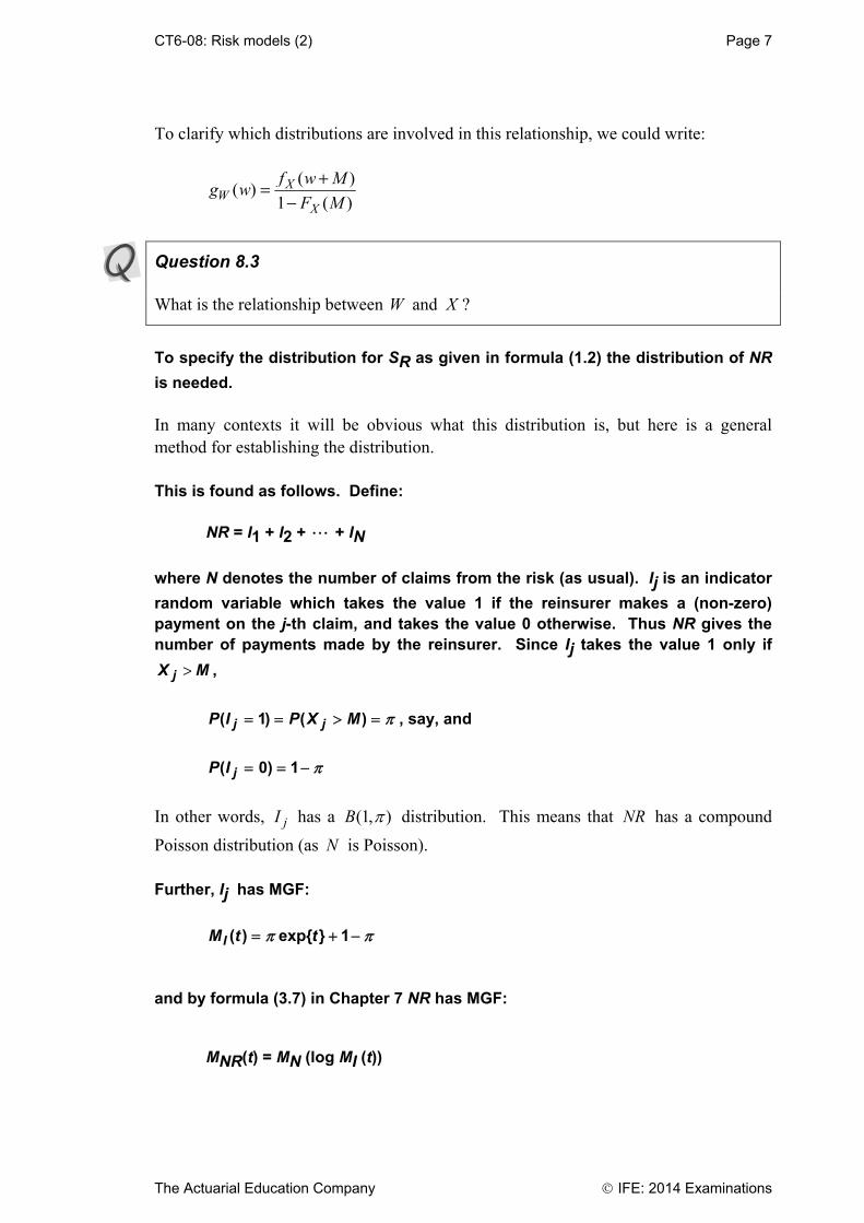
CT6-08: Risk models (2) Page 7
The Actuarial Education Company IFE: 2014 Examinations
To clarify which distributions are involved in this relationship, we could write:
( )( )
1 ( )X
WX
f w Mg w
F M
+=-
Question 8.3
What is the relationship between W and X ?
To specify the distribution for SR as given in formula (1.2) the distribution of NR
is needed. In many contexts it will be obvious what this distribution is, but here is a general method for establishing the distribution. This is found as follows. Define:
NR = I1 + I2 + + IN
where N denotes the number of claims from the risk (as usual). Ij is an indicator
random variable which takes the value 1 if the reinsurer makes a (non-zero) payment on the j-th claim, and takes the value 0 otherwise. Thus NR gives the number of payments made by the reinsurer. Since Ij takes the value 1 only if
>jX M ,
P I P X Mj j( ) ( ) 1 , say, and
P I j( ) 0 1
In other words, I j has a B( , )1 distribution. This means that NR has a compound
Poisson distribution (as N is Poisson). Further, Ij has MGF:
M t tI ( ) exp 1
and by formula (3.7) in Chapter 7 NR has MGF:
MNR(t) = MN (log MI (t))

Page 8 CT6-08: Risk models (2)
IFE: 2014 Examinations The Actuarial Education Company
Question 8.4
If N has a Poisson( ) distribution, and half of the claims exceed the excess-of-loss
retention limit, show that NR has a Poisson(½ ) distribution.
Example Continuing the above example and using formula (1.2) as the model for SR, it can
be seen that SR has a compound Poisson distribution with Poisson parameter
0 2 10 2. . Individual claims, Wi, have density function:
g(w) = ( )
1 ( )
f w M
F M
+-
= 0.0005/0.2 = 0.0025, for 0 < w < 400
ie Wi is uniformly distributed on (0,400). [ ] 200iE W = , 2[ ] 53,333.33iE W = and
3[ ] 16,000,000iE W = , giving the same result as before.
We haven’t worked out these precise quantities before, but if you multiply these figures by 2 (the Poisson parameter of SR ), you get ( ) 400RE S = , var( ) 106,667RS = and
skew( ) , ,SR 32 000 000 , which agree with the answers obtained previously.
Thus, there are two ways to specify and evaluate the distribution of SR.
The next question is a long question that uses a lot of the ideas we’ve covered so far. You will need to do some preliminary calculations in order to work out the answers.

CT6-08: Risk models (2) Page 29
The Actuarial Education Company IFE: 2014 Examinations
Chapter 8 Summary Collective risk model with reinsurance In the collective risk model, individual claims can be subject to a reinsurance agreement, either proportional or excess of loss. Recall from Chapter 7 that, under the collective risk model, the aggregate claim amount S is given by: 1 2 NS X X X
where iX is the amount of the thi claim and N is the total number of claims.
If reinsurance is in place, the insurer’s aggregate claims net of reinsurance can be represented as: 1 2I NS Y Y Y
where iY is the amount of the thi claim paid by the insurer and N is defined as above.
Now IS has a compound distribution and note that we can apply the formulae for the
moments as given on Page 16 of the Tables, substituting Y for X . The reinsurer’s aggregate claims can be represented as: 1 2R NS Z Z Z
where iZ is the amount of the thi claim paid by the reinsurer and N is defined as above.
Now RS has a compound distribution and note that we can apply the formulae for the
moments as given on Page 16 of the Tables, substituting Z for X .

Page 30 CT6-08: Risk models (2)
IFE: 2014 Examinations The Actuarial Education Company
Under non-proportional (or excess of loss) reinsurance, some of the claims may fall below the retention level M . If this is the case, then some of the iZ will be zero. An alternative
way of expressing the reinsurer’s aggregate claims is as: 1 2R NRS W W W
where | 0i i iW Z Z and NR is the number of non-zero claims, ie the number of claims
in which the reinsurer is involved. Individual risk model The individual risk model considers the payments made under each risk (eg policy) separately. The risks are assumed to be independent and the number of risks is fixed over the period of insurance cover. The aggregate claim random variable S may be written as: 1 2 nS Y Y Y= + + +
where Yj denotes the claim amount under the j th risk and n denotes the number of
risks. The number of claims from the j th risk is either 0 or 1, which means that the individual
risk model is often used to model life insurance risks (where the maximum number of claims is 1). The probability of a claim arising from the j th risk is q j . If a claim does arise from the
thj risk, the mean claim amount is j and the variance of the claim amount is 2j .
Each jY is the sum of a random number (0 or 1) of random claim amounts. Hence each
jY has a compound binomial distribution.
If, for a group of n risks, the probability of a claim is fixed and the claim amounts are i.i.d, then the individual risk model is equivalent to a collective risk model where S has a
compound binomial distribution with ,N bin n q .
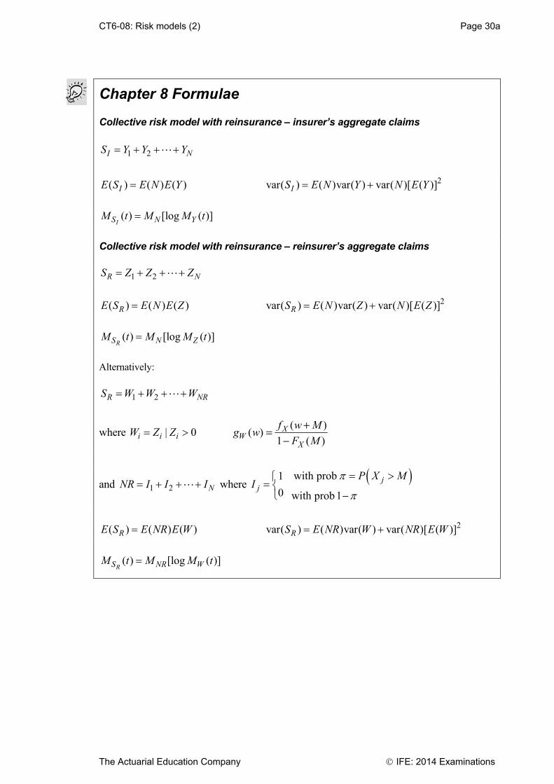
CT6-08: Risk models (2) Page 30a
The Actuarial Education Company IFE: 2014 Examinations
Chapter 8 Formulae
Collective risk model with reinsurance – insurer’s aggregate claims
1 2I NS Y Y Y
( ) ( ) ( )IE S E N E Y 2var( ) ( )var( ) var( )[ ( )]IS E N Y N E Y
( ) [log ( )]IS N YM t M M t
Collective risk model with reinsurance – reinsurer’s aggregate claims
1 2R NS Z Z Z
( ) ( ) ( )RE S E N E Z 2var( ) ( )var( ) var( )[ ( )]RS E N Z N E Z
( ) [log ( )]RS N ZM t M M t
Alternatively:
1 2R NRS W W W
where | 0i i iW Z Z ( )
( )1 ( )
XW
X
f w Mg w
F M
+=-
and 1 2 NNR I I I where with prob1
0 with prob1
jj
P X MI
( ) ( ) ( )RE S E NR E W 2var( ) ( )var( ) var( )[ ( )]RS E NR W NR E W
( ) [log ( )]RS NR WM t M M t
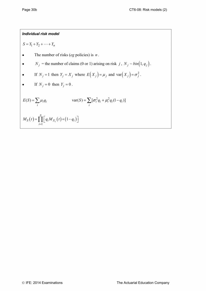
Page 30b CT6-08: Risk models (2)
IFE: 2014 Examinations The Actuarial Education Company
Individual risk model
1 2 nS Y Y Y
The number of risks (eg policies) is n .
jN = the number of claims (0 or 1) arising on risk j , 1,j jN bin q .
If 1jN then j jY X where j jE X and 2var j jX .
If 0jN then 0jY .
( ) i ii
E S q 2 2var( ) [ (1 )]i i i i ii
S q q qs m= + -Â
1
1i
n
S i X ii
M t q M t q
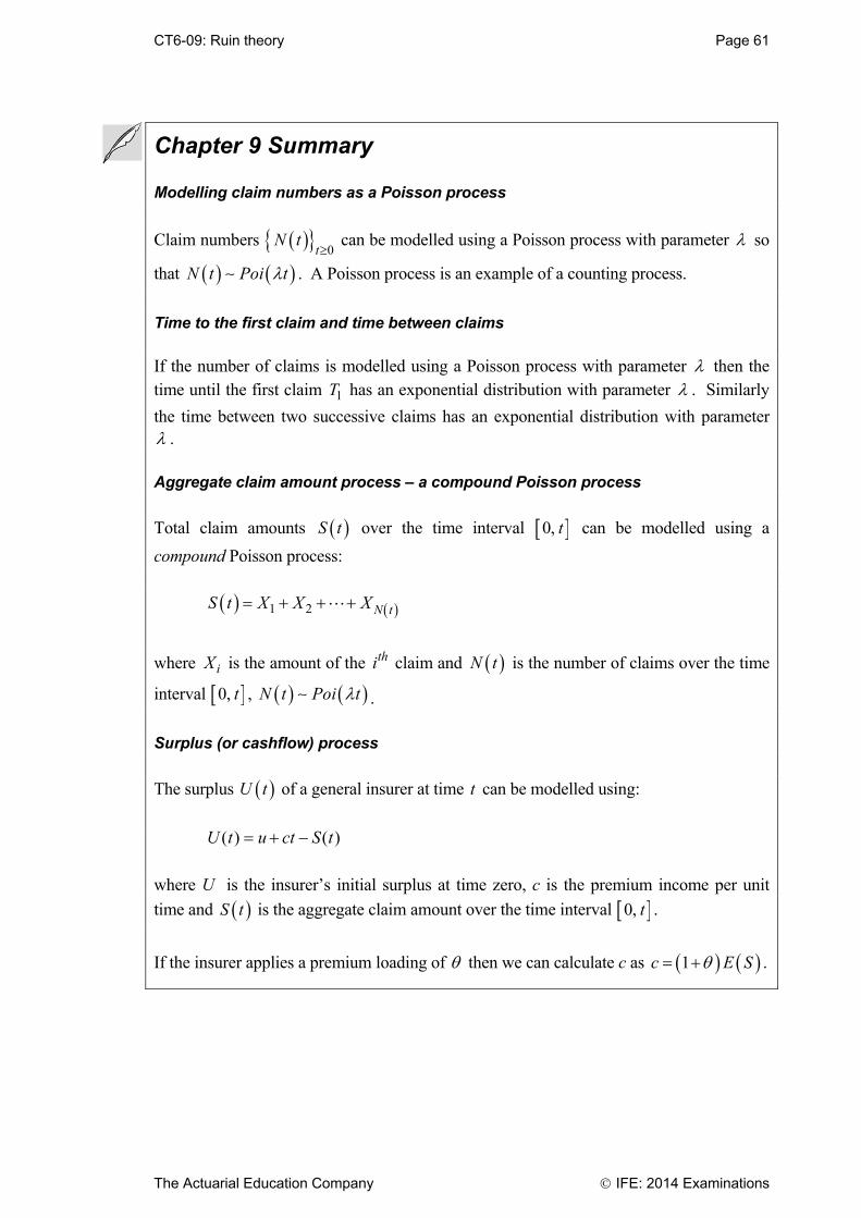
CT6-09: Ruin theory Page 61
The Actuarial Education Company IFE: 2014 Examinations
Chapter 9 Summary Modelling claim numbers as a Poisson process
Claim numbers 0tN t
can be modelled using a Poisson process with parameter so
that N t Poi t . A Poisson process is an example of a counting process.
Time to the first claim and time between claims If the number of claims is modelled using a Poisson process with parameter then the time until the first claim 1T has an exponential distribution with parameter . Similarly
the time between two successive claims has an exponential distribution with parameter . Aggregate claim amount process – a compound Poisson process
Total claim amounts S t over the time interval 0, t can be modelled using a
compound Poisson process:
1 2 N tS t X X X
where iX is the amount of the thi claim and N t is the number of claims over the time
interval 0, t , N t Poi t . Surplus (or cashflow) process
The surplus U t of a general insurer at time t can be modelled using:
U t u ct S t( ) ( ) where U is the insurer’s initial surplus at time zero, c is the premium income per unit
time and S t is the aggregate claim amount over the time interval 0, t .
If the insurer applies a premium loading of then we can calculate c as 1c E S .
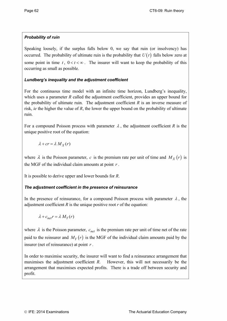
Page 62 CT6-09: Ruin theory
IFE: 2014 Examinations The Actuarial Education Company
Probability of ruin Speaking loosely, if the surplus falls below 0, we say that ruin (or insolvency) has
occurred. The probability of ultimate ruin is the probability that U t falls below zero at
some point in time t , 0 t . The insurer will want to keep the probability of this occurring as small as possible. Lundberg’s inequality and the adjustment coefficient For the continuous time model with an infinite time horizon, Lundberg’s inequality, which uses a parameter R called the adjustment coefficient, provides an upper bound for the probability of ultimate ruin. The adjustment coefficient R is an inverse measure of risk, ie the higher the value of R, the lower the upper bound on the probability of ultimate ruin. For a compound Poisson process with parameter , the adjustment coefficient R is the unique positive root of the equation:
( )Xcr M r
where l is the Poisson parameter, c is the premium rate per unit of time and ( )XM r is
the MGF of the individual claim amounts at point r . It is possible to derive upper and lower bounds for R. The adjustment coefficient in the presence of reinsurance In the presence of reinsurance, for a compound Poisson process with parameter , the adjustment coefficient R is the unique positive root r of the equation:
( )net Yc r M r
where l is the Poisson parameter, netc is the premium rate per unit of time net of the rate
paid to the reinsurer and ( )YM r is the MGF of the individual claim amounts paid by the
insurer (net of reinsurance) at point r . In order to maximise security, the insurer will want to find a reinsurance arrangement that maximises the adjustment coefficient R. However, this will not necessarily be the arrangement that maximises expected profits. There is a trade off between security and profit.

CT6-09: Ruin theory Page 63
The Actuarial Education Company IFE: 2014 Examinations
Effect of changes in parameter values on the probability of ruin The probability of ultimate ruin decreases if the insurer’s premium loading is increased or if the insurer’s initial surplus U is increased. This is because the insurer has more of a buffer against claims. An increase in the value of the Poisson parameter will not affect the probability of
ultimate ruin since the expected aggregate claims E S E X , the variance of
aggregate claims 2var S E X and the premium rate 1 E X all increase
proportionately in line with . However, it will reduce the time it takes for ruin to occur.
An increase in the variance var X of the individual claim amounts will increase the
probability of ruin as it will increase the uncertainty associated with the aggregate claims process without any corresponding increase in premium.
An increase in the expected individual claim amount E X will increase the probability
of ruin. The expected aggregate claims and the premium rate both increase
proportionately in line with E X , however the variance of the aggregate claims amount
increases disproportionately since 22var varS E X X E X . The
variance of the aggregate claim amount increases in line with 2E X .
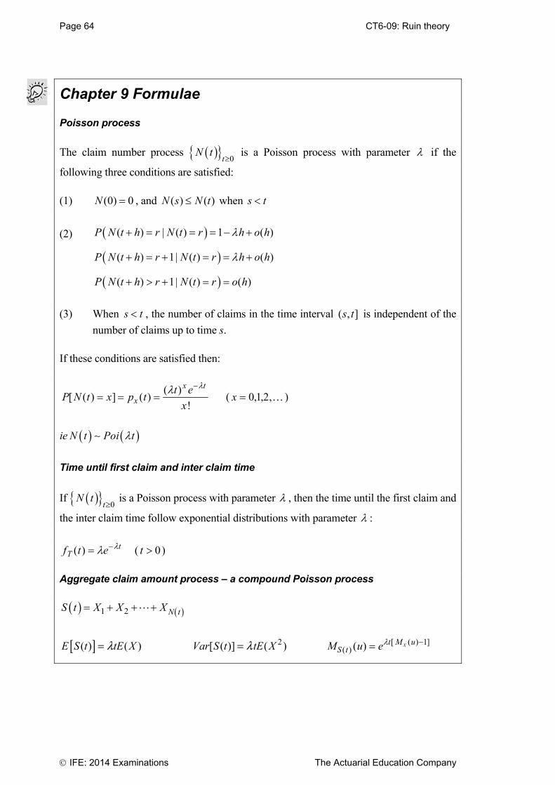
Page 64 CT6-09: Ruin theory
IFE: 2014 Examinations The Actuarial Education Company
Chapter 9 Formulae Poisson process
The claim number process 0tN t
is a Poisson process with parameter if the
following three conditions are satisfied: (1) (0) 0N , and ( ) ( )N s N t when s t
(2)
( ) | ( ) 1 ( )
( ) 1| ( ) ( )
( ) 1| ( ) ( )
P N t h r N t r h o h
P N t h r N t r h o h
P N t h r N t r o h
(3) When s t , the number of claims in the time interval ( , ]s t is independent of the
number of claims up to time s. If these conditions are satisfied then:
P N t x p tt e
xx
x t
[ ( ) ] ( )( )
!
( x 0 1 2, , , )
ie N t Poi t
Time until first claim and inter claim time
If 0tN t
is a Poisson process with parameter , then the time until the first claim and
the inter claim time follow exponential distributions with parameter :
f t eTt( ) ( t 0)
Aggregate claim amount process – a compound Poisson process
1 2 N tS t X X X
[ ]( ) ( )l=E S t tE X 2[ ( )] ( )Var S t tE Xl= M u eS tt M uX
( )[ ( ) ]( ) 1
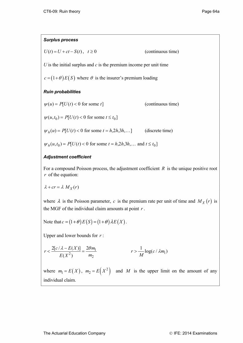
CT6-09: Ruin theory Page 64a
The Actuarial Education Company IFE: 2014 Examinations
Surplus process
( ) ( )U t U ct S t , t 0 (continuous time)
U is the initial surplus and c is the premium income per unit time
1c E S where is the insurer’s premium loading
Ruin probabilities ( ) [ ( ) ]u P U t t 0 for some (continuous time)
( , ) [ ( ) ]u t P U t t t0 00 for some
h u P U t t h h h( ) [ ( ) , , , ] 0 2 3 for some (discrete time)
h u t P U t t h h h t t( , ) [ ( ) , , , ]0 00 2 3 for some and Adjustment coefficient For a compound Poisson process, the adjustment coefficient R is the unique positive root r of the equation: cr M rX ( )
where l is the Poisson parameter, c is the premium rate per unit of time and ( )XM r is
the MGF of the individual claim amounts at point r .
Note that ( ) ( ) ( ) ( )1 1c E S E Xq q l= + = + .
Upper and lower bounds for r :
12
2
22[ / ( )]
( )
mc E Xr
mE X
r
Mc m
11log( / )
where 1m E X , 22m E X and M is the upper limit on the amount of any
individual claim.
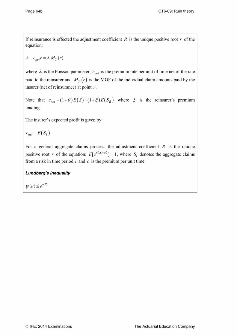
Page 64b CT6-09: Ruin theory
IFE: 2014 Examinations The Actuarial Education Company
If reinsurance is effected the adjustment coefficient R is the unique positive root r of the equation:
( )net Yc r M r
where l is the Poisson parameter, netc is the premium rate per unit of time net of the rate
paid to the reinsurer and ( )YM r is the MGF of the individual claim amounts paid by the
insurer (net of reinsurance) at point r .
Note that 1 1net Rc E S E S where is the reinsurer’s premium
loading. The insurer’s expected profit is given by:
net Ic E S
For a general aggregate claims process, the adjustment coefficient R is the unique
positive root r of the equation: E er S ci[ ]( ) 1, where Si denotes the aggregate claims
from a risk in time period i and c is the premium per unit time. Lundberg’s inequality
( ) Ruu e
CT6-10: Generalised linear models Page 1
The Actuarial Education Company IFE: 2014 Examinations
Chapter 10
Generalised linear models
Syllabus objectives (vii) 1. Be familiar with the principles of Multiple Linear Regression and the
Normal Linear Model. 2. Define an exponential family of distributions. Show that the following
distributions may be written in this form: binomial, Poisson, exponential, gamma, normal.
3. State the mean and variance for an exponential family, and define the
variance function and the scale parameter. Derive these quantities for the distributions in 2.
4. Explain what is meant by the link function and the canonical link
function, referring to the distributions in 2. 5. Explain what is meant by a variable, a factor taking categorical values
and an interaction term. Define the linear predictor, illustrating its form for simple models, including polynomial models and models involving factors.
6. Define the deviance and scaled deviance and state how the parameters of
a GLM may be estimated. Describe how a suitable model may be chosen by using an analysis of deviance and by examining the significance of the parameters.
7. Define the Pearson and deviance residuals and describe how they may
be used. 8. Apply statistical tests to determine the acceptability of a fitted model:
Pearson’s Chi-square test and the likelihood ratio test.
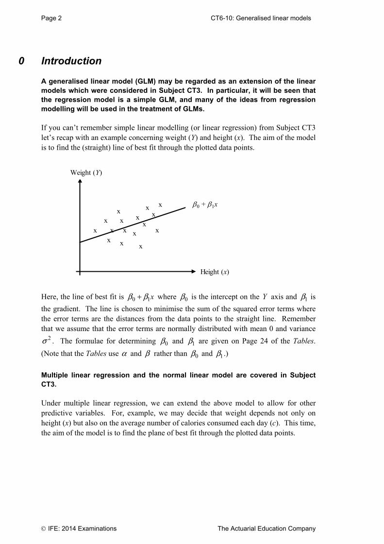
Page 2 CT6-10: Generalised linear models
IFE: 2014 Examinations The Actuarial Education Company
0 Introduction
A generalised linear model (GLM) may be regarded as an extension of the linear models which were considered in Subject CT3. In particular, it will be seen that the regression model is a simple GLM, and many of the ideas from regression modelling will be used in the treatment of GLMs. If you can’t remember simple linear modelling (or linear regression) from Subject CT3 let’s recap with an example concerning weight (Y) and height (x). The aim of the model is to find the (straight) line of best fit through the plotted data points.
Weight (Y)
Height (x)
x
x
x
xx
x
x
x
x
xx
xx
x
x
x 0 + 1x
Here, the line of best fit is 0 1xb b+ where 0b is the intercept on the Y axis and 1b is
the gradient. The line is chosen to minimise the sum of the squared error terms where the error terms are the distances from the data points to the straight line. Remember that we assume that the error terms are normally distributed with mean 0 and variance
2s . The formulae for determining 0b and 1b are given on Page 24 of the Tables.
(Note that the Tables use a and b rather than 0b and 1b .)
Multiple linear regression and the normal linear model are covered in Subject CT3. Under multiple linear regression, we can extend the above model to allow for other predictive variables. For, example, we may decide that weight depends not only on height (x) but also on the average number of calories consumed each day (c). This time, the aim of the model is to find the plane of best fit through the plotted data points.

CT6-10: Generalised linear models Page 3
The Actuarial Education Company IFE: 2014 Examinations
Weight (Y)
Height (x)
0 + 1x + c
Calories (c)
x
x
x
xx
x
x
x
x
xx
xx
x
x
x
xx
x
x
x
x x
x
x
x
x
xx
x
Here, the plane of best fit is 0 1 2x cb b b+ + .
Note that, under multiple regression, we still assume that the error terms are normally
distributed with mean 0 and variance 2s . We could extend this multiple regression model to allow for even more predictive variables (eg average number of minutes of exercise, sex) but this becomes difficult to represent graphically! The essential difference for GLMs is that we now allow the distribution of the data to be non-normal. This is particularly important in actuarial work where the data very often do not have a normal distribution. For example, in mortality, the Poisson distribution is used in modelling the force of mortality, xm , and the
binomial distribution for the initial rate of mortality, qx. In general insurance, the
Poisson distribution is often used for modelling the claim frequency and the gamma or lognormal distribution for the claim severity. Claim severity is just another term for the size of a claim, whereas claim frequency refers to the rate at which claims are received.

Page 4 CT6-10: Generalised linear models
IFE: 2014 Examinations The Actuarial Education Company
GLMs are widely used both in general and life insurance. They are used to: 1) determine which rating factors to use (rating factors are measurable or categorical factors that are used as proxies for risk in setting premiums) 2) estimate an appropriate premium to charge for a particular policy given the level of risk present. For example, in motor insurance, there are a large number of factors that may be may be used as proxies for the level of risk (type of car driven, age of driver, number of years past driving experience, etc). We can use a GLM both to determine which of these factors are significant to the assessment of risk (and hence which should be included) and to suggest an appropriate premium to charge for a risk that represents a particular combination of these factors.
Question 10.1
Suggest rating factors that an insurance company may consider in the pricing of a single life annuity contract.
The aims of a data analysis exercise are usually to decide which variables or factors are important predictors for the risk being considered, and then to quantify the relationship between the predictors and the risk in order to assess appropriate premium levels. The objective covers the basic theory of GLMs which is necessary for applications such as those mentioned above. GLMs relate a variable (called the response variable) which you want to predict, to variables or factors (called predictors, covariates or independent variables) about which you have information. In the multiple regression example on Page 3, the response variable is weight (Y) and the covariates (or predictive variables) are height (x) and average number of daily calories (c). We will see later that, more precisely, a GLM uses the sample data to define the relationship between the mean m of the response variable and the covariates.
In order to do this, it is necessary first to define the distribution of the response. Then the covariates can be related to the response allowing for the random variation of the data. Thus, the first step is to consider the general form of distributions (known as exponential families) which are used in GLMs. The exponential family of distributions as defined in the next section includes the normal, Poisson, binomial, gamma and exponential distributions.
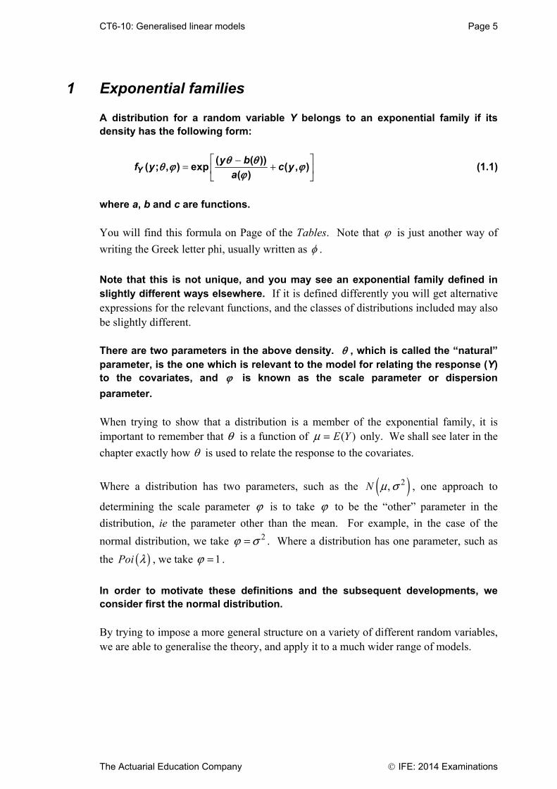
CT6-10: Generalised linear models Page 5
The Actuarial Education Company IFE: 2014 Examinations
1 Exponential families
A distribution for a random variable Y belongs to an exponential family if its density has the following form:
È ˘-= +Í ˙Î ˚
( ( ))( ; , ) exp ( , )
( )Yy b
f y c ya
q qq j jj
(1.1)
where a, b and c are functions. You will find this formula on Page of the Tables. Note that is just another way of
writing the Greek letter phi, usually written as .
Note that this is not unique, and you may see an exponential family defined in slightly different ways elsewhere. If it is defined differently you will get alternative expressions for the relevant functions, and the classes of distributions included may also be slightly different. There are two parameters in the above density. , which is called the “natural” parameter, is the one which is relevant to the model for relating the response (Y) to the covariates, and is known as the scale parameter or dispersion
parameter. When trying to show that a distribution is a member of the exponential family, it is important to remember that q is a function of ( )m = E Y only. We shall see later in the
chapter exactly how is used to relate the response to the covariates.
Where a distribution has two parameters, such as the ( )2,N m s , one approach to
determining the scale parameter j is to take j to be the “other” parameter in the
distribution, ie the parameter other than the mean. For example, in the case of the
normal distribution, we take 2j s= . Where a distribution has one parameter, such as
the ( )Poi l , we take 1j = .
In order to motivate these definitions and the subsequent developments, we consider first the normal distribution. By trying to impose a more general structure on a variety of different random variables, we are able to generalise the theory, and apply it to a much wider range of models.

Page 6 CT6-10: Generalised linear models
IFE: 2014 Examinations The Actuarial Education Company
1.1 Normal distribution
È ˘- -= Í ˙Í ˙Î ˚
È ˘Ê ˆ-Í ˙Á ˜ Ê ˆË ¯Í ˙= - +Á ˜Í ˙Ë ¯Í ˙
Í ˙Î ˚
2
22
2
22
2 2
1 ( )( ; , ) exp
22
2 1exp log2
2
Yy
f y
yy
mq jsps
mmps
s s
which is in the form of (1.1), with:
=
=
=
=
Ê ˆ= - +Á ˜
Ë ¯
2
2
2
( )
( ) 2
1( , ) log2
2
a
b
yc y
q m
j s
j j
j pff
Thus, the natural parameter for the normal distribution is and the scale
parameter is 2s .
Note that we could alternatively have taken j s= and ( ) 2a j j= . There is no unique
parameterisation. For members of an exponential family, we want to be able to find formulae for the mean and variance of the distribution from the general parameters. Consider now the log-likelihood function, =( ; , ) log( ( ; , ))Yl y f yq j q j . We will use
this later when we consider estimation for GLMs. At the moment we need two well-known results from statistical theory:
È ˘ =Í ˙Î ˚
0l
E∂∂q
and È ˘È ˘ Ê ˆÍ ˙+ =Í ˙ Á ˜Ë ¯Í ˙Í ˙Î ˚ Î ˚
22
20
l lE E
∂ ∂∂q∂q

CT6-10: Generalised linear models Page 7
The Actuarial Education Company IFE: 2014 Examinations
By applying these results to 1.1, it can be shown that the mean and variance of Y are: E Y b( ) ( ) and var( ) ( ) ( )Y a bj q= ¢¢
where the dash denotes differentiation with respect to . These formulae can also be found on Page 27 of the Tables.
Question 10.2
Prove these two results for a member of an exponential family, using the results given above.
These are very important results which we now consider in more detail. Firstly, considering the normal distribution, we can derive the mean and variance:
b( ) 2
2 so E Y b( ) ( )
a( ) so 2var( ) ( ) ( )Y a bj q j s= = =¢¢
So these do give us the results that we expect for the normal distribution.
Question 10.3
Show that if we reparameterise the normal distribution using 2 , we still get the
same results for the mean and variance of the distribution.
In general, note that the mean does not depend on j , so when predicting Y it is
q that is of importance. Also, the variance of the data has two components: one that involves the scale parameter, and the other that determines the way the variance depends on the mean. For the normal distribution, the variance of Y does not depend on the mean (since b ( ) 1), but for other distributions we
shall see that the variance does depend on the mean. For example, for the Poisson distribution the mean and variance are both equal to the parameter . So knowing the mean of a Poisson distribution tells us the variance as well.

Page 8 CT6-10: Generalised linear models
IFE: 2014 Examinations The Actuarial Education Company
To emphasise the dependence on the mean, the variance is often written as var( ) ( ) ( )Y a Vj m= , where the “variance function” is defined as
V b( ) ( )
Note that the variance function does not give the variance directly, unless ( ) 1j =a .
We now consider other distributions as exponential families. Note that we use f, in a slight abuse of notation, for both continuous and discrete distributions. You will have seen this style of notation before in Subject CT3. The alternative notation is to use p x( ) for a probability function and f x( ) for a density function.
Provided that you make it clear what you are doing, you may use either notation.
1.2 Poisson distribution
f ye
yy yY
y( ; , )
!exp[ log log !]
which is in the form of (1.1), with:
log
, ( )
( )
( , ) log !
1 1 so that a
b e
c y y
Thus, the natural parameter for the Poisson distribution is logm , the mean is
E Y b e( ) ( ) and the variance function is V b e( ) ( ) . The
variance function tells us that the variance is proportional to the mean. We can see that the variance is actually equal to the mean since a( ) 1.
Question 10.4
Could we reparameterise the Poisson distribution using 2j = , say?

CT6-10: Generalised linear models Page 9
The Actuarial Education Company IFE: 2014 Examinations
1.3 Binomial distribution
This is slightly more awkward to deal with, since we have to first divide the
binomial random variable by n. Thus, suppose Z ~ binomial ( , )n m . Let Y = Z
n,
so that Z = nY. The distribution of Z is -Ê ˆ= -Á ˜Ë ¯
( ; , ) (1 )z n zZ
nf z
zq j m m and by
substituting for z, the distribution of Y is:
-Ê ˆ= -Á ˜Ë ¯
È ˘Ê ˆ= + - - +Í ˙Á ˜Ë ¯Î ˚
È ˘Ê ˆÊ ˆ Ê ˆ= + - +Í ˙Á ˜ Á ˜Á ˜- Ë ¯Ë ¯Ë ¯Í ˙Î ˚
( ; , ) (1 )
exp ( log (1 )log(1 )) log
exp log log(1 ) log1
ny n nyY
nf y
ny
nn y y
ny
nn y
ny
q j m m
m m
m mm
which is in the form of (1.1), with:
Ê ˆ
= Á ˜-Ë ¯log
1
mqm
(note that the inverse of this is =+1
e
e
q
qm )
= nj
= 1( )a j
j
= +( ) log(1 )b eqq
Ê ˆ
= Á ˜Ë ¯( , ) log
nc y
nyj
The reason for all this is that q is a function of m , the distribution mean only.
However, the binomial distribution as we typically quote it: ( ),Bin n p does not have m
as one of its parameters. So we will start by considering ( , )Bin n m , which does have
m as a parameter, but has mean nm . We then divide this by n to get a distribution
with m in its probability function and which also has mean m .
Note that nj = , the “other” parameter in the distribution (ie the parameter other than
the mean).

Page 10 CT6-10: Generalised linear models
IFE: 2014 Examinations The Actuarial Education Company
Question 10.5
Verify that the formulae given in the Core Reading are correct.
Thus, the natural parameter for the binomial distribution is Ê ˆÁ ˜-Ë ¯
log1
mm
, the mean
is:
E Y be
e[ ] ( )
1
and the variance function is:
V be
e( ) ( )
( )( )
11
2.
We can get the second derivative of b( ) most easily by writing ( ) 1( ) 1 1b eqq
-= - +¢ .
Question 10.6
Are these the results you would expect?
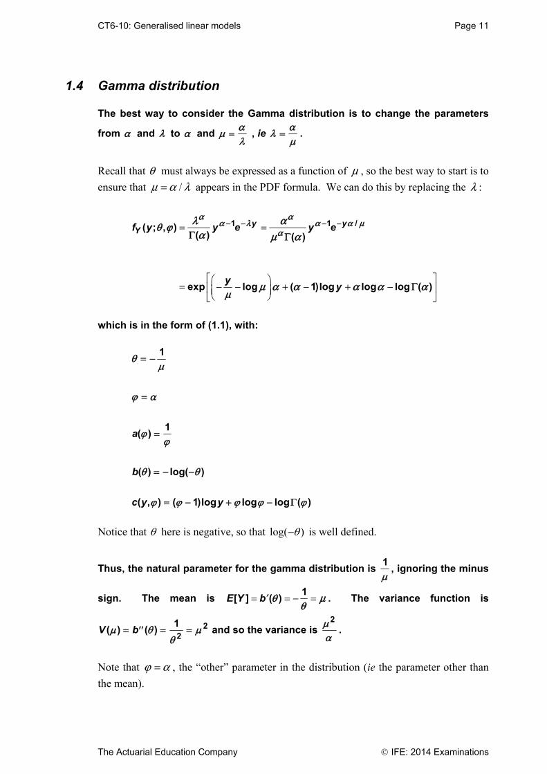
CT6-10: Generalised linear models Page 11
The Actuarial Education Company IFE: 2014 Examinations
1.4 Gamma distribution
The best way to consider the Gamma distribution is to change the parameters
from and to and
, ie
.
Recall that q must always be expressed as a function of m , so the best way to start is to
ensure that /m a l= appears in the PDF formula. We can do this by replacing the l :
- - - -= =
È ˘Ê ˆ= - - + - + -Í ˙Á ˜Ë ¯Î ˚
1 1 /( ; , )( ) ( )
exp log ( 1)log log log ( )
y yYf y y e y e
yy
a aa l a a m
al aq ja m a
m a a a a am
G G
G
which is in the form of (1.1), with:
1
1
1
a
b
c y y
( )
( ) log( )
( , ) ( )log log log ( )
Notice that here is negative, so that log( ) is well defined.
Thus, the natural parameter for the gamma distribution is 1
, ignoring the minus
sign. The mean is 1
[ ] ( )E Y b q mq
= = - =¢ . The variance function is
V b( ) ( )
12
2 and so the variance is
2.
Note that j a= , the “other” parameter in the distribution (ie the parameter other than
the mean).

Page 12 CT6-10: Generalised linear models
IFE: 2014 Examinations The Actuarial Education Company
Finally, the lognormal distribution is often used, for example in general insurance to model the distribution of claim sizes. This can be incorporated in the framework of GLMs since if Y ~ lognormal, log ~Y normal. Thus, if the
lognormal distribution is to be used, the data should first be logged and then the normal modelling distribution can be applied.
Question 10.7
Show that the exponential distribution can be written in the form of a member of the exponential family.
Ssyllabus objective (vii)2 requires that you can show that the binomial, Poisson, exponential, gamma and normal distributions are members of the exponential family. Make sure that you can do this as it is a common exam question. Our study of GLMs requires that the distribution we use is a member of the exponential family. Using the exponential form also makes finding the log likelihood function (to obtain MLEs) much easier.
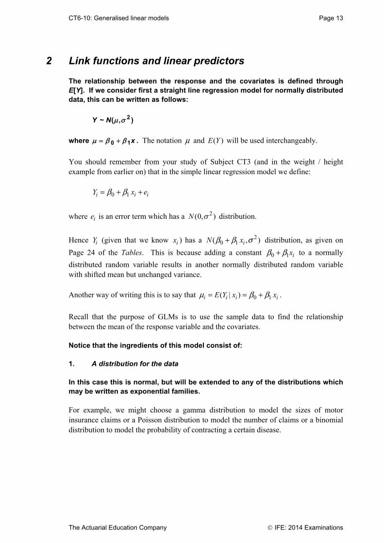
CT6-10: Generalised linear models Page 13
The Actuarial Education Company IFE: 2014 Examinations
2 Link functions and linear predictors
The relationship between the response and the covariates is defined through E[Y]. If we consider first a straight line regression model for normally distributed data, this can be written as follows:
Y N~ ( , ) 2
where 0 1x . The notation m and ( )E Y will be used interchangeably.
You should remember from your study of Subject CT3 (and in the weight / height example from earlier on) that in the simple linear regression model we define:
0 1i i iY x eb b= + +
where ei is an error term which has a N ( , )0 2 distribution.
Hence Yi (given that we know ix ) has a 20 1( , )iN xb b s+ distribution, as given on
Page 24 of the Tables. This is because adding a constant 0 1 ixb b+ to a normally
distributed random variable results in another normally distributed random variable with shifted mean but unchanged variance. Another way of writing this is to say that 0 1( | )i i i iE Y x xm b b= = + .
Recall that the purpose of GLMs is to use the sample data to find the relationship between the mean of the response variable and the covariates. Notice that the ingredients of this model consist of: 1. A distribution for the data In this case this is normal, but will be extended to any of the distributions which may be written as exponential families. For example, we might choose a gamma distribution to model the sizes of motor insurance claims or a Poisson distribution to model the number of claims or a binomial distribution to model the probability of contracting a certain disease.

Page 14 CT6-10: Generalised linear models
IFE: 2014 Examinations The Actuarial Education Company
2. A “linear predictor” The linear predictor h is a function of the covariates. In this case it is
= +0 1xh b b .
Note that is the Greek letter “eta”.
For example, if the response variable is weight, this linear predictor would be appropriate for a model where we thought the only covariate was height, x. Note that a linear predictor is linear in the parameters 0b and 1b . It does not have to
be linear in the covariates, for example 20 1xh b b= + is also a linear predictor.
3. A “link function” It is necessary to connect the mean response to the linear predictor. In this case this relationship is a straightforward equality: E[Y] = linear predictor.
In the above example, we had 0 1i i ixm h b b= = + .
In general we take some function of the mean response and this function is called the link function. Putting 2. and 3. together, we have in general the relationship: g( )
where g is the link function and is the linear predictor.
The link function, like its name suggests, is the missing link. Remember that what we are trying to do in a GLM is determine a relationship between the mean of the response
variable and the covariates. By setting the link function ( )g m h= , then, assuming that
the link function is invertible, we can make the mean m the subject of the formula:
( )1gm h-=
The notation is not straightforward to get to grips with. An example may help.
CT6-10: Generalised linear models Page 15
The Actuarial Education Company IFE: 2014 Examinations
Example Suppose that we are trying to model the number of claims on car insurance policies. The response variable, iY , is the number of claims on Policy i. We decide that a
Poisson distribution would be appropriate:
( )i iY Poi m
Consider a model where we believe that the only covariate is the age, ix , of the
policyholder. The linear predictor is i ixh a b= + .
A link function that is commonly used with the Poisson distribution (see Page 27 of the Tables) is:
( ) logg m m= We set this equal to the linear predictor:
( ) logi i i ig xm m h a b= = = +
Now we invert the formula so that im is the subject of the formula:
( ) ( )exp expi i ixm h a b= = +
We now have a relationship between the mean of the response variable and the covariate.
Question 10.8
Why is the link function ( ) logg m m= appropriate to the Poisson distribution? Hint
– consider the range of values that it results in im taking.
We discuss link functions and linear predictors in more detail further on.

Page 16 CT6-10: Generalised linear models
IFE: 2014 Examinations The Actuarial Education Company
In order to define a GLM, we need to specify all three of the above components. In practice, the distribution of the data is usually specified at the outset (often defined by the data), the linear predictor may be chosen according to what is thought appropriate or convenient, and then the best model structure found by looking at a range of linear predictors. Of course, these are not rules which must be adhered to: it may be that it is possible that more than one distribution could be appropriate, and these should be investigated before making a final decision. It could be unclear which link function should be used, and again a range of functions can be investigated.
Key information The three components of a GLM are: 1) a distribution for the data (Poisson, exponential, gamma, normal or binomial) 2) a linear predictor (a function of the covariates that is linear in the parameters) 3) a link function (that links the mean of the response variable to the linear predictor).
In order for you to understand how these three components fit together, we give a couple of further examples below.
CT6-10: Generalised linear models Page 17
The Actuarial Education Company IFE: 2014 Examinations
Example Suppose that we are setting up a model to predict the pass rate for a particular student in a particular actuarial exam. We might expect there to be many factors that affect whether a student is likely to pass or not. We might decide to set up a three-factor model, so that the probability of passing is a function of: (i) the number of assignments N submitted by the student (a value from 0 to 4) (ii) the student’s mark on the mock exam S (on a scale from 0 to 100) (iii) whether the student had attended tutorials or not (Yes/No). We might then decide to use the linear predictor: 1 2i N Sh a b b= + +
where N is the number of assignments submitted, S is the mark on the mock exam, and ia takes one value for those attending tutorials and a different value for those who
do not. We now need a link function. h here will not necessarily take a value in the
interval (0, 1). Depending on the values of ia , 1b and 2b , h might take any value. If
we use the link function ( ) log1
gmmm
Ê ˆ= Á ˜-Ë ¯
and set this equal to the linear predictor h ,
we have log1
m hm
Ê ˆ=Á ˜-Ë ¯
. We invert this function to make m the subject to give
( ) 111
1 1
ee
e e
hh
h hm--
-= = = ++ +
. We can now see that m will lie in the range from
zero to one, and so can be used as a pass rate. We now use maximum likelihood estimation to estimate the four parameter values: Ya ,
Na (the a parameters corresponding to having attended tutorials and not having
attended tutorials, respectively), 1b (the parameter for the number of assignments) and
2b (the parameter for the mock mark). To do this we need (ideally) the actual exam
results of a large sample of students who fall into each of the categories.
Page 18 CT6-10: Generalised linear models
IFE: 2014 Examinations The Actuarial Education Company
Having done this for a set of data, we might come up with the following parameter values for the linear predictor:
Y 1501. N 3196. 1 05459 . 2 0 0251 .
We can now use the linear predictor and link function to predict pass rates for groups of students with a particular characteristic. For example, for a student who attends tutorials, submits three assignments and scores 65% on the mock, we have: 1.501 0.5459 3 0.0251 65 1.7682h = - + ¥ + ¥ =
We now use the inverse of the link function to calculate m :
( ) 11.76821 0.8542em--= + =
So the model predicts an 85% probability of passing for a student in this situation. So in this particular situation, the linear predictor is 1 2i N Sh a b b= + + and the link
function is ( ) log1
gmmm
Ê ˆ= Á ˜-Ë ¯
.
Question 10.9
Using the model outlined above, answer the following questions. (i) What is the predicted pass probability for a student who attends tutorials,
submits three assignments and scores 60% on the mock exam? (ii) How much would the probability go up by if the fourth assignment were
submitted? (iii) What is the highest pass probability for someone who does not attend tutorials? (iv) Can anyone get a probability of 0 or 1 under this model? If not, what are the
minimum and maximum scores? (v) What is the underlying probability distribution?
CT6-10: Generalised linear models Page 19
The Actuarial Education Company IFE: 2014 Examinations
Example A statistician is analysing data on truancy rates for different school pupils. She believes that the number of unexplained days off school in a year (ie those not due to sickness etc) for a particular pupil may have a Poisson distribution with parameter . However,
she believes that there are a number of factors that may affect , for example: age of
pupil, ethnic group, and sex. She builds a linear model based on these characteristics, using data from a large group of pupils. Her model will take the form:
i j x
where x age , and and are numerical variables corresponding to the different
characteristics for ethnic group and sex respectively. She has collected the data shown in the table below. Each figure gives the average number of unexplained absences in a year for 16 different groups of pupils, all the pupils within each group having the same characteristics. Solution
Average number of unexplained absences in a year
Age last birthday
8 10 12 14
White Male 1.8 2.0 6.3 14.1
Female 0.5 1.6 5.0 16.2
Non-white Male 2.1 7.5 25.5 72.0
Female 2.8 6.2 19.6 68.2
By carrying out a maximum likelihood estimation analysis, she calculates the values of the parameters that fit the model best. As a result she can find a value of for any
particular pupil, which she can use to find the appropriate Poisson parameter using the link function. In this case she needs a function that converts a number that may take
any value into a positive number (since the Poisson parameter must always be
positive). So for example she could use the link function g( ) log , so that when
this is set equal to the linear predictor h and inverted, e . This will give her a
positive value for , which she can use for her Poisson parameter.
Page 20 CT6-10: Generalised linear models
IFE: 2014 Examinations The Actuarial Education Company
So she might come up with the following values for the parameters:
W 2 64. NW 114. M 326. F 354. 0 64.
where W White , NW Non-white, M Male , F Female . She can now use the model to predict possible truancy rates for students with particular characteristics. The link function g( ) log is called the canonical link function for the Poisson
distribution. Canonical just means the accepted form of the function. It is a “natural” function to use, and will often give sensible results. In fact it is not compulsory to use the canonical link function and there may be situations where a different link function is more appropriate. Each case must be judged on its merits.
Question 10.10
What is the expected number of unexplained days’ absence for a white female pupil who is 12 years old?
We now consider the link function and the linear predictor in a little more depth.
2.1 Link functions
Technically, it is necessary for the link function to be differentiable and invertible in order to fit a model. An invertible function is one that is “one-to-one”, so that for any value of there is a
unique value of . We have seen already that it is important to be able to invert the
link function in order to use the model to make predictions about the future. Beyond these basic requirements, there are a number of functions that are appropriate for the distributions above. For each distribution, the natural, or canonical, link function is defined by g( ) ( ) .
Remember that q is the natural parameter for the exponential family form and that q is a function of the mean of the distribution m .

CT6-10: Generalised linear models Page 21
The Actuarial Education Company IFE: 2014 Examinations
Hence the canonical link function for each of the above cases is: Normal Identity =( )g m m
Poisson Log =( ) logg m m
Binomial Logit Ê ˆ
= Á ˜-Ë ¯( ) log
1g
mmm
Gamma Inverse (Reciprocal) = 1( )g m
m.
On Page 11, we showed that 1qm
= - for the gamma distribution. The minus sign is
dropped in the canonical link function. This doesn’t affect anything since constants will be absorbed into the parameters in the linear predictor (see below). The canonical link functions are given on Page 27 of the Tables. These link functions work well for each of the above distributions, but it is not obligatory that they be used in each case. For example, you could use the identity link function in conjunction with the Poisson distribution, you could use the log link function for data which had a gamma distribution, and so on. However, you need to consider the implications of the choice of the link function on the possible values for . For example, if the data have a Poisson
distribution then must be positive. If you use the log link function, then
log and e . Thus, is guaranteed to be positive, whatever value
(positive or negative) the linear predictor takes. The same is not true if you use the identity link function. Other link functions exist, and can be quite complex, for specific modelling purposes. As a basis for actuarial applications, the above four functions are often sufficient.
Question 10.11
Find the inverse of the link function ( ) log1
gmmm
Ê ˆ= Á ˜-Ë ¯
by setting it equal to h and
comment on why this might be an appropriate link function for the binomial distribution.

Page 22 CT6-10: Generalised linear models
IFE: 2014 Examinations The Actuarial Education Company
2.2 Linear predictor
The covariates (also known as explanatory or predictor variables), enter the model through the linear predictor. This is also where the parameters occur which have to be estimated. In the case of a straight line for a single explanatory variable x, the linear predictor is 0 1 x , and to fit this model it is necessary to
estimate the parameters 0 and 1. In this case, the actual value of x matters.
An example of a variable of this type which occurs very commonly in actuarial applications is the age of the policyholder. There are two types of covariate: variables and factors. A variable is a type of covariate whose real numerical value enters the linear predictor directly, such as age (x). Other examples of variables in a car insurance context are annual mileage and number of years for which a driving licence has been held. The other main type of covariate is a factor, which takes a categorical value. For example, the sex of the policyholder is either male or female, which constitutes a factor with 2 categories (or levels). This type of covariate can be parameterised so that the linear predictor has a term 1 for a male, and a term 2 for a female.
Other examples of factors in a car insurance context are postcode and car type. Thus, a model which includes an age effect and an effect for the sex of the policyholder could have a linear predictor +i xa b
where 1i = for a male and 2i = for a female. You may be wondering how this linear predictor has been determined. Let’s look at this in more detail. A useful way of constructing linear predictors that involve more than one covariate (or main effect) is to start by summing the linear predictors for each individual covariate. Here, the linear predictor for “age” is 0 1xh b b= + and the linear
predictor for “sex” is , 1, 2i ih a= = . Summing these gives:
0 1 ixh b b a= + +
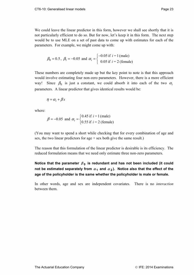
CT6-10: Generalised linear models Page 23
The Actuarial Education Company IFE: 2014 Examinations
We could leave the linear predictor in this form, however we shall see shortly that it is not particularly efficient to do so. But for now, let’s keep it in this form. The next step would be to use MLE on a set of past data to come up with estimates for each of the parameters. For example, we might come up with:
0 0.5b = , 1 0.05b = - and 0.05 if = 1 (male)
0.05 if = 2 (female)ii
ia
-Ï= ÌÓ
These numbers are completely made up but the key point to note is that this approach would involve estimating four non-zero parameters. However, there is a more efficient way! Since 0b is just a constant, we could absorb it into each of the two ia
parameters. A linear predictor that gives identical results would be: i xh a b= +
where:
0.05b = - and 0.45 if = 1 (male)
0.55 if = 2 (female)ii
ia Ï
= ÌÓ
(You may want to spend a short while checking that for every combination of age and sex, the two linear predictors for age + sex both give the same result.) The reason that this formulation of the linear predictor is desirable is its efficiency. The reduced formulation means that we need only estimate three non-zero parameters. Notice that the parameter 0 is redundant and has not been included (it could
not be estimated separately from 1 and 2 ). Notice also that the effect of the
age of the policyholder is the same whether the policyholder is male or female. In other words, age and sex are independent covariates. There is no interaction between them.
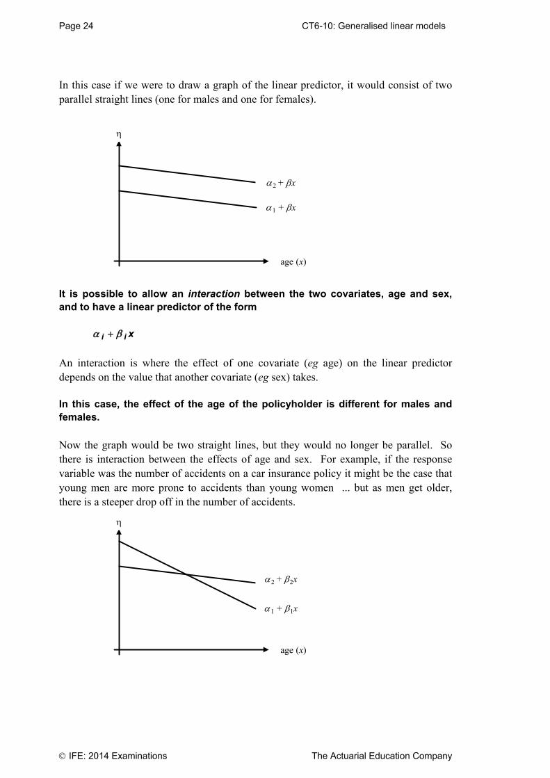
Page 24 CT6-10: Generalised linear models
IFE: 2014 Examinations The Actuarial Education Company
In this case if we were to draw a graph of the linear predictor, it would consist of two parallel straight lines (one for males and one for females).
age (x)
1 + x
2 + x
It is possible to allow an interaction between the two covariates, age and sex, and to have a linear predictor of the form i i x
An interaction is where the effect of one covariate (eg age) on the linear predictor depends on the value that another covariate (eg sex) takes. In this case, the effect of the age of the policyholder is different for males and females. Now the graph would be two straight lines, but they would no longer be parallel. So there is interaction between the effects of age and sex. For example, if the response variable was the number of accidents on a car insurance policy it might be the case that young men are more prone to accidents than young women ... but as men get older, there is a steeper drop off in the number of accidents.
age (x)
1 + 1x
2 + 2x
CT6-10: Generalised linear models Page 25
The Actuarial Education Company IFE: 2014 Examinations
An interaction term is denoted using a “.” notation. For example an interaction between age and sex would be denoted as “age.sex”. An interaction term never appears on its own. It is always accompanied by the main effects. The notation that is used to denote the main effects and the interaction term is “*”. For example: age*sex = age + sex + age.sex Let’s now consider how we would construct the linear predictor i i xa b+ for this
model. We start by summing the linear predictors for each of the three terms: age, sex and age.sex separately. We already know that the linear predictor for age alone is
0 1xh b b= + and that the linear predictor for sex alone is , 1, 2i ih a= = . We also need
a linear predictor for the interaction effect ( )0 1 . , 1, 2ix ih b b a= + = . Note that the dot
notation here does not mean multiply. We have just written it in this format for now to indicate an interaction. We add the three of these together:
( )0 1 0 1 .i ix xh b b a b b a= + + + +
We could then use MLE on a set of past data to come up with estimates based on past data for each of the parameters. For example, these might be:
0 0.5b = , 1 0.05b = - , 0.05 if = 1 (male)
0.05 if = 2 (female)ii
ia
-Ï= ÌÓ
and interaction terms:
00.35 if = 1 (male)
.0.05 if = 2 (female)i
i
ib a Ï
= ÌÓ
and 10.15 if = 1 (male)
.0.02 if = 2 (female)i
i
ib a
-Ï= Ì-Ó
Note that this approach, which is rather artificial, would involve estimating eight non-zero parameters. However, there is a more efficient way! We can combine the parameters 0b , ia and 0 . ib a (these terms are not attached to an x in the linear
predictor). Similarly, we can combine the terms 1b and 1 . ib a (these terms are
attached to an x in the linear predictor).
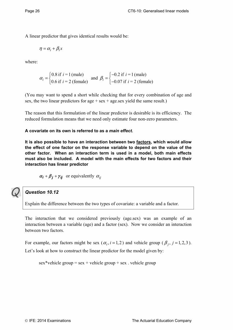
Page 26 CT6-10: Generalised linear models
IFE: 2014 Examinations The Actuarial Education Company
A linear predictor that gives identical results would be: i i xh a b= +
where:
0.8 if = 1 (male)
0.6 if = 2 (female)ii
ia Ï
= ÌÓ
and 0.2 if = 1 (male)
0.07 if = 2 (female)ii
ib
-Ï= Ì-Ó
(You may want to spend a short while checking that for every combination of age and sex, the two linear predictors for age + sex + age.sex yield the same result.) The reason that this formulation of the linear predictor is desirable is its efficiency. The reduced formulation means that we need only estimate four non-zero parameters. A covariate on its own is referred to as a main effect. It is also possible to have an interaction between two factors, which would allow the effect of one factor on the response variable to depend on the value of the other factor. When an interaction term is used in a model, both main effects must also be included. A model with the main effects for two factors and their interaction has linear predictor
+ +i j ija b g or equivalently ija
Question 10.12
Explain the difference between the two types of covariate: a variable and a factor.
The interaction that we considered previously (age.sex) was an example of an interaction between a variable (age) and a factor (sex). Now we consider an interaction between two factors. For example, our factors might be sex ( , 1, 2i ia = ) and vehicle group ( , 1, 2,3j jb = ).
Let’s look at how to construct the linear predictor for the model given by: sex*vehicle group = sex + vehicle group + sex . vehicle group

CT6-10: Generalised linear models Page 27
The Actuarial Education Company IFE: 2014 Examinations
We start by summing the linear predictors for each of the three terms: sex, vehicle group and sex . vehicle group type separately. We already know that the linear predictor for sex alone is , 1, 2i ih a= = . Similarly, the linear predictor for vehicle
group alone is , 1, 2,3j jh b= = . We also need a linear predictor for the interaction
effect . 1, 2 and 1, 2,3i j i jh a b= = = . Note once again that the dot notation here does
not mean multiply. We have just written it in this format for now to indicate an interaction. We add the three of these together: .i j i jh a b a b= + +
An alternative (and more commonly used) notation for the interaction term which depends on both i and j is ijg , so that i j ijh a b g= + + .
We could then use MLE on a set of past data to come up with estimates based on past data for each of the parameters. For example, these might be:
0.45 if = 1 (male)
0.55 if = 2 (female)ii
ia Ï
= ÌÓ
and
0.05 if = 1
0.03 if = 2
0.04 if = 3
j
j
j
j
bÏÔ
= ÌÔ-Ó
and the interaction term:
0.05 if 1and = 1
0.02 if 1and = 2
0.01if 1and = 3
0.06 if 2 and = 1
0.03 if 2 and = 2
0.03 if 2 and = 3
ij
i j
i j
i j
i j
i j
i j
g
=ÏÔ =ÔÔ- =Ô
= Ì =ÔÔ =ÔÔ- =Ó
Note that this approach, which is rather artificial, would involve estimating eleven non-zero parameters. However, there is a more efficient way! We can sum the above three terms into one.
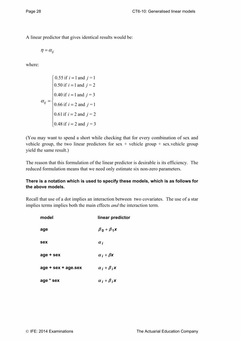
Page 28 CT6-10: Generalised linear models
IFE: 2014 Examinations The Actuarial Education Company
A linear predictor that gives identical results would be: ijh a=
where:
0.55 if 1and = 1
0.50 if 1 and = 2
0.40 if 1 and = 3
0.66 if 2 and = 1
0.61if 2 and = 2
0.48 if 2 and = 3
ij
i j
i j
i j
i j
i j
i j
a
=ÏÔ =ÔÔ =Ô
= Ì =ÔÔ =ÔÔ
=Ó
(You may want to spend a short while checking that for every combination of sex and vehicle group, the two linear predictors for sex + vehicle group + sex.vehicle group yield the same result.) The reason that this formulation of the linear predictor is desirable is its efficiency. The reduced formulation means that we need only estimate six non-zero parameters. There is a notation which is used to specify these models, which is as follows for the above models. Recall that use of a dot implies an interaction between two covariates. The use of a star implies terms implies both the main effects and the interaction term. model linear predictor age 0 1 x
sex i
age + sex i x
age + sex + age.sex i i x
age * sex i i x
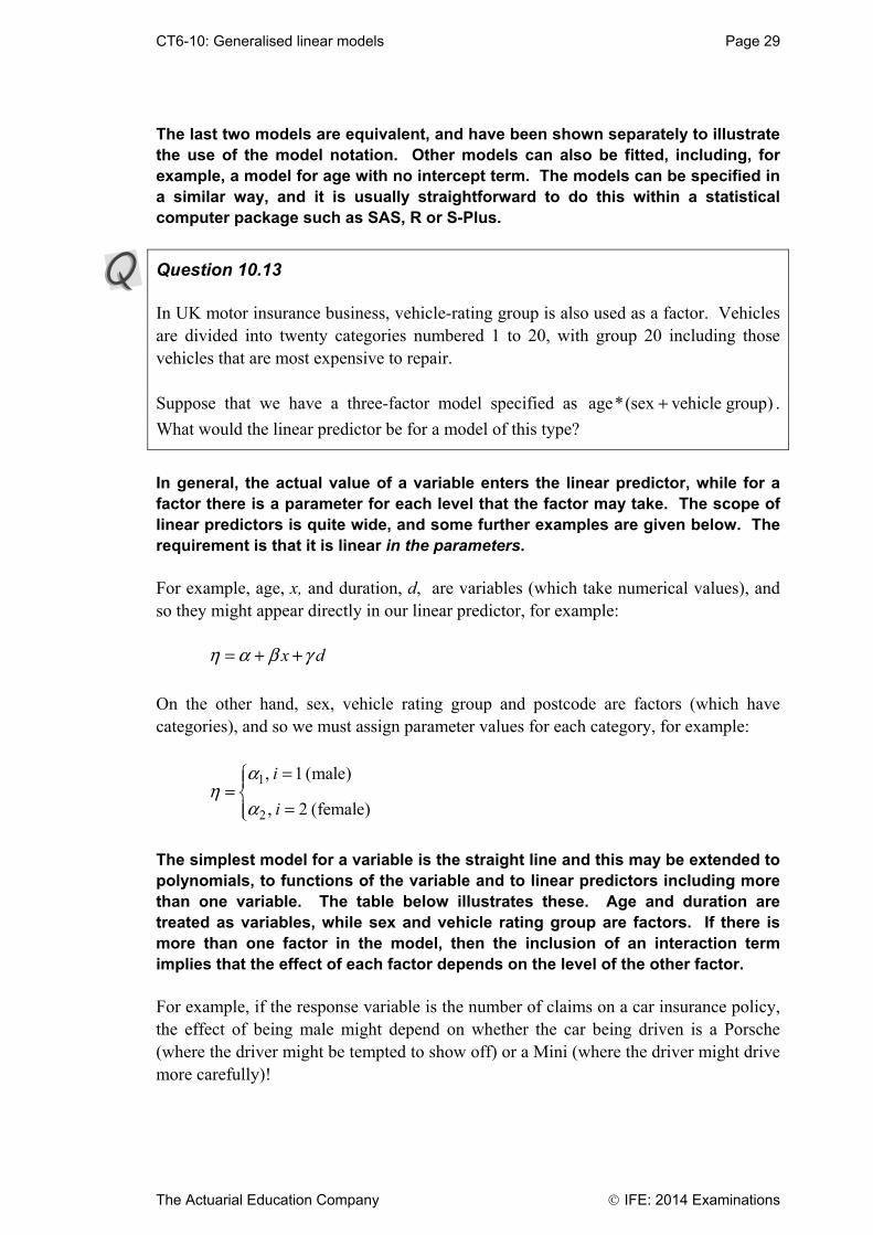
CT6-10: Generalised linear models Page 29
The Actuarial Education Company IFE: 2014 Examinations
The last two models are equivalent, and have been shown separately to illustrate the use of the model notation. Other models can also be fitted, including, for example, a model for age with no intercept term. The models can be specified in a similar way, and it is usually straightforward to do this within a statistical computer package such as SAS, R or S-Plus.
Question 10.13
In UK motor insurance business, vehicle-rating group is also used as a factor. Vehicles are divided into twenty categories numbered 1 to 20, with group 20 including those vehicles that are most expensive to repair. Suppose that we have a three-factor model specified as age*(sex vehicle group)+ .
What would the linear predictor be for a model of this type?
In general, the actual value of a variable enters the linear predictor, while for a factor there is a parameter for each level that the factor may take. The scope of linear predictors is quite wide, and some further examples are given below. The requirement is that it is linear in the parameters. For example, age, x, and duration, d, are variables (which take numerical values), and so they might appear directly in our linear predictor, for example: x dh a b g= + +
On the other hand, sex, vehicle rating group and postcode are factors (which have categories), and so we must assign parameter values for each category, for example:
1
2
, 1 (male)
, 2 (female)
i
i
ah
a
=ÏÔ= Ì=ÔÓ
The simplest model for a variable is the straight line and this may be extended to polynomials, to functions of the variable and to linear predictors including more than one variable. The table below illustrates these. Age and duration are treated as variables, while sex and vehicle rating group are factors. If there is more than one factor in the model, then the inclusion of an interaction term implies that the effect of each factor depends on the level of the other factor. For example, if the response variable is the number of claims on a car insurance policy, the effect of being male might depend on whether the car being driven is a Porsche (where the driver might be tempted to show off) or a Mini (where the driver might drive more carefully)!

Page 30 CT6-10: Generalised linear models
IFE: 2014 Examinations The Actuarial Education Company
Further examples of linear predictors are as follows: model linear predictor age 0 1 x
age + age2 0 1 22 x x
age + duration 0 1 1 2 2 x x
log(age) +0 1log xb b
sex i
vehicle rating group j
sex + vehicle rating group i j
sex * vehicle rating group i j ij or ija
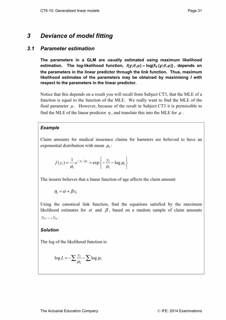
CT6-10: Generalised linear models Page 31
The Actuarial Education Company IFE: 2014 Examinations
3 Deviance of model fitting
3.1 Parameter estimation
The parameters in a GLM are usually estimated using maximum likelihood estimation. The log-likelihood function, l y f yY( ; , ) log( ( ; , )) , depends on
the parameters in the linear predictor through the link function. Thus, maximum likelihood estimates of the parameters may be obtained by maximising l with respect to the parameters in the linear predictor. Notice that this depends on a result you will recall from Subject CT3, that the MLE of a function is equal to the function of the MLE. We really want to find the MLE of the final parameter . However, because of the result in Subject CT3 it is permissible to
find the MLE of the linear predictor , and translate this into the MLE for .
Example Claim amounts for medical insurance claims for hamsters are believed to have an exponential distribution with mean im :
/1( ) exp logi iy i
i ii i
yf y e m m
m m- Ï ¸
= = - -Ì ˝Ó ˛
The insurer believes that a linear function of age affects the claim amount: i ixh a b= +
Using the canonical link function, find the equations satisfied by the maximum likelihood estimates for a and b , based on a random sample of claim amounts
1, , ny y .
Solution The log of the likelihood function is:
log logii
i
yL m
m= - -Â Â

Page 32 CT6-10: Generalised linear models
IFE: 2014 Examinations The Actuarial Education Company
The canonical link function is ( ) 1i
ig m
m= . By setting this equal to the linear predictor,
ie 1
ii
hm
= , this enables us to write the log-likelihood function in terms of a and b .
log log
( ) log( )
i i i
i i i
L y
y x x
h h
a b a b
= - +
= - + + +
 Â
 Â
We can now differentiate this with respect to a and b :
1
log ii
L yxa a b
∂ = - +∂ +Â Â
log ii i
i
xL x y
xb a b∂ = - +∂ +Â Â
So the equations satisfied by the MLEs of a and b are:
1
0ii
yxa b
- + =+Â Â
and: 0ii i
i
xx y
xa b- + =
+Â Â
These may not be particularly easy to solve without computer assistance.
Question 10.14
You are given the following data for hamsters’ medical claims, using the model above: age ix (months) 4 8 10 11 17
claim amount (£) 50 52 119 41 163 Write down (but do not try to solve) the equations for the MLE’s for a and b in this
case.
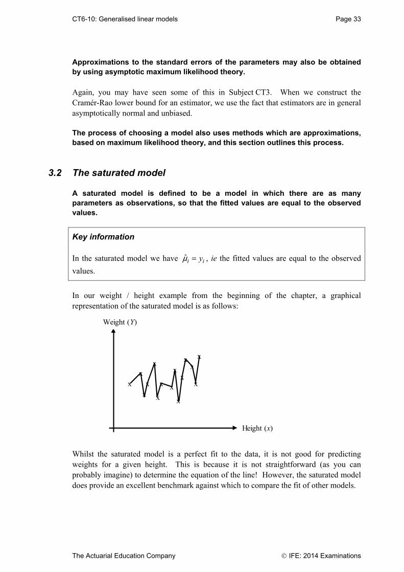
CT6-10: Generalised linear models Page 33
The Actuarial Education Company IFE: 2014 Examinations
Approximations to the standard errors of the parameters may also be obtained by using asymptotic maximum likelihood theory. Again, you may have seen some of this in Subject CT3. When we construct the Cramér-Rao lower bound for an estimator, we use the fact that estimators are in general asymptotically normal and unbiased. The process of choosing a model also uses methods which are approximations, based on maximum likelihood theory, and this section outlines this process.
3.2 The saturated model
A saturated model is defined to be a model in which there are as many parameters as observations, so that the fitted values are equal to the observed values.
Key information In the saturated model we have ˆi iym = , ie the fitted values are equal to the observed
values.
In our weight / height example from the beginning of the chapter, a graphical representation of the saturated model is as follows:
Weight (Y)
Height (x)
xx
xx
x
x
x
x
xx
xx
x
x
x
Whilst the saturated model is a perfect fit to the data, it is not good for predicting weights for a given height. This is because it is not straightforward (as you can probably imagine) to determine the equation of the line! However, the saturated model does provide an excellent benchmark against which to compare the fit of other models.
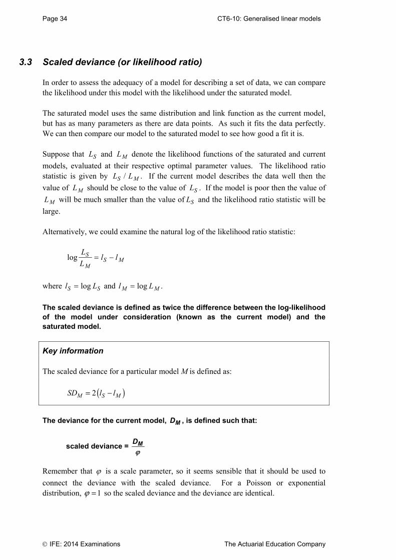
Page 34 CT6-10: Generalised linear models
IFE: 2014 Examinations The Actuarial Education Company
3.3 Scaled deviance (or likelihood ratio)
In order to assess the adequacy of a model for describing a set of data, we can compare the likelihood under this model with the likelihood under the saturated model. The saturated model uses the same distribution and link function as the current model, but has as many parameters as there are data points. As such it fits the data perfectly. We can then compare our model to the saturated model to see how good a fit it is. Suppose that LS and LM denote the likelihood functions of the saturated and current
models, evaluated at their respective optimal parameter values. The likelihood ratio statistic is given by L LS M/ . If the current model describes the data well then the
value of LM should be close to the value of LS . If the model is poor then the value of
LM will be much smaller than the value of LS and the likelihood ratio statistic will be
large. Alternatively, we could examine the natural log of the likelihood ratio statistic:
logL
Ll lS
MS M
where l LS S log and l LM M log .
The scaled deviance is defined as twice the difference between the log-likelihood of the model under consideration (known as the current model) and the saturated model.
Key information The scaled deviance for a particular model M is defined as:
( )2M S MSD l l= -
The deviance for the current model, DM , is defined such that:
scaled deviance = DM
Remember that is a scale parameter, so it seems sensible that it should be used to
connect the deviance with the scaled deviance. For a Poisson or exponential distribution, 1j = so the scaled deviance and the deviance are identical.
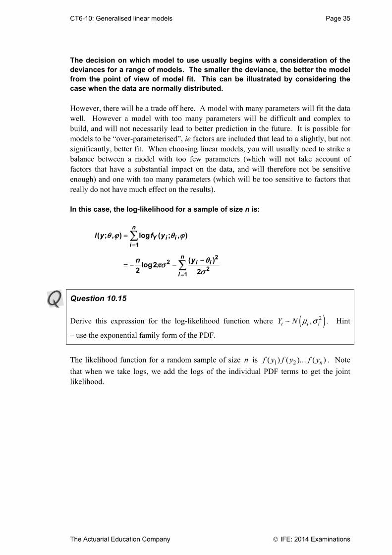
CT6-10: Generalised linear models Page 35
The Actuarial Education Company IFE: 2014 Examinations
The decision on which model to use usually begins with a consideration of the deviances for a range of models. The smaller the deviance, the better the model from the point of view of model fit. This can be illustrated by considering the case when the data are normally distributed. However, there will be a trade off here. A model with many parameters will fit the data well. However a model with too many parameters will be difficult and complex to build, and will not necessarily lead to better prediction in the future. It is possible for models to be “over-parameterised”, ie factors are included that lead to a slightly, but not significantly, better fit. When choosing linear models, you will usually need to strike a balance between a model with too few parameters (which will not take account of factors that have a substantial impact on the data, and will therefore not be sensitive enough) and one with too many parameters (which will be too sensitive to factors that really do not have much effect on the results). In this case, the log-likelihood for a sample of size n is:
=
=
=
-= - -
Â
Â
1
22
21
( ; , ) log ( ; , )
( )log2
2 2
n
Y i ii
ni i
i
l y f y
yn
q j q j
qpss
Question 10.15
Derive this expression for the log-likelihood function where ( )2,i i iY N m s . Hint
– use the exponential family form of the PDF.
The likelihood function for a random sample of size n is f y f y f yn( ) ( )... ( )1 2 . Note
that when we take logs, we add the logs of the individual PDF terms to get the joint likelihood.

Page 36 CT6-10: Generalised linear models
IFE: 2014 Examinations The Actuarial Education Company
For the saturated model, the parameter i is estimated by yi , and so the second
term disappears. Thus, the scaled deviance (twice the difference between the values of the log-likelihood under the current and saturated models) is
i
ni iy
1
2
2
( )
where i is the fitted value for the current model. The deviance (remembering
that the scale parameter 2 ), is the well-known residual sum of squares:
i
n
i iy
1
2( )
This is why the deviance is defined with a factor of two in it, so that for the normal model the deviance is equal to the usual sum of squares.
3.4 Likelihood ratio test
Thus, it can be seen that the deviance is a measure of the fit of the model. For
normally distributed data, the scaled deviance has a 2 distribution. So far, we
have ignored the problem of the scale parameter, which must also be estimated. For normal data, the usual procedure is to take ratios of sum-of-squares and use F-tests (as in the analysis of variance). Remember that we used F -tests to compare variances in our study of Analysis of Variance in Subject CT3. In the case of data that are not normally distributed, the scale parameter may be known (for example, for the Poisson distribution 1), and the deviance has
only approximately (actually asymptotically) a 2 distribution. For these
reasons, the common procedure is to compare two models by looking at the
difference in the deviance and comparing this with the 2 distribution.
To be more precise, it’s the absolute difference between the scaled deviances that is
compared with 2c .
A significant value (at the 5% level) for a 2 distribution with degrees of
freedom is, approximately, 2 . Thus, if we want to decide if model 2 (which has
p parameters and deviance 2S ) is a significant improvement over model 1 (which
has q parameters and deviance 1S ), we can compare 1 2S S- with ( )-2 p q .
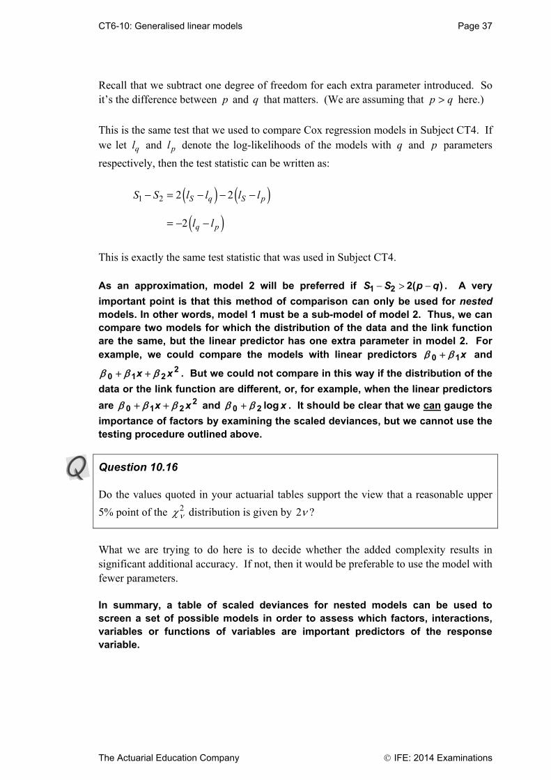
CT6-10: Generalised linear models Page 37
The Actuarial Education Company IFE: 2014 Examinations
Recall that we subtract one degree of freedom for each extra parameter introduced. So it’s the difference between p and q that matters. (We are assuming that >p q here.)
This is the same test that we used to compare Cox regression models in Subject CT4. If we let ql and pl denote the log-likelihoods of the models with q and p parameters
respectively, then the test statistic can be written as:
( ) ( )( )
1 2 2 2
2
- = - - -
= - -
S q S p
q p
S S l l l l
l l
This is exactly the same test statistic that was used in Subject CT4. As an approximation, model 2 will be preferred if 1 2 2( )S S p q- > - . A very
important point is that this method of comparison can only be used for nested models. In other words, model 1 must be a sub-model of model 2. Thus, we can compare two models for which the distribution of the data and the link function are the same, but the linear predictor has one extra parameter in model 2. For example, we could compare the models with linear predictors 0 1 x and
0 1 22 x x . But we could not compare in this way if the distribution of the
data or the link function are different, or, for example, when the linear predictors
are 0 1 22 x x and 0 2 log x . It should be clear that we can gauge the
importance of factors by examining the scaled deviances, but we cannot use the testing procedure outlined above.
Question 10.16
Do the values quoted in your actuarial tables support the view that a reasonable upper
5% point of the 2 distribution is given by 2 ?
What we are trying to do here is to decide whether the added complexity results in significant additional accuracy. If not, then it would be preferable to use the model with fewer parameters. In summary, a table of scaled deviances for nested models can be used to screen a set of possible models in order to assess which factors, interactions, variables or functions of variables are important predictors of the response variable.

Page 38 CT6-10: Generalised linear models
IFE: 2014 Examinations The Actuarial Education Company
3.5 Example
To illustrate the use of the deviance in model choice, we consider a set of data relating to motor claims. There are three factors: policyholder age (pa), vehicle age (va) and car rating group (cg). These data were used in the book, “Generalised Linear Models” by P McCullagh and J Nelder, which is probably the most widely used reference book in this area. We use the analysis from that book. The scaled deviances for the complete range of possible models are shown in the table below. Model Deviance Degrees of Differences Freedom 1 638.32 122 81.13 7 pa 557.19 115
226.5 3 pa+cg 330.65 112
204.1 3 pa+cg+va 126.51 109
34.32 21 pa+cg+va+pa.cg 92.191 88 18.77 21 pa+cg+va+pa.cg+pa.va 73.416 67 3.89 9 pa+cg+va+pa.cg+pa.va+cg.va 69.524 58 69.524 58 pa+cg+va+pa.cg+pa.va+cg.va+pa.cg.vg 0 0 In the original data sample, there were: 8 different age groups for the policyholder’s age 4 different car vehicle groups 4 different possible vehicle age ranges This gave a total of 128 different cells of data. Each cell contained an average claim amount together with the number of claims on which the average was based. 5 of the cells were empty, ie there were no data for that particular combination of policyholder age, car age and car group.

CT6-10: Generalised linear models Page 39
The Actuarial Education Company IFE: 2014 Examinations
Model “1” consists of a single value for the average claim size constant for all different groups. There is a single parameter to estimate, and so the deviance (the sum of the squares of the differences between the actual and predicted average claim amount) is large. In this model the total number of degrees of freedom is 122. This is the total number of non-empty cells, less one. This is analogous to the number of degrees of freedom used in our chi square tests in Subject CT3. As we add more factors to the model, the number of parameters fitted becomes larger, and the number of degrees of freedom becomes smaller. For example, Model “pa” adds a factor for the policyholder’s age. There were eight different age groups, so eight parameters to estimate, or seven more than the constant model. The number of degrees of freedom is reduced by seven. Model “pa + cg” adds a factor for car group. At first glance it would seem that we are adding four more parameters (to represent the four car groups) and so the number of degrees of freedom should be reduced by four. In fact, this is incorrect. When adding a new main effect, it is always possible to absorb one of the parameters into the others. Effectively we are setting one parameter to zero. We saw a good example of this earlier in the chapter when we were formulating the linear predictor earlier for age + sex. We managed to absorb the 0b parameter into each of the ia parameters, effectively setting
0b to 0.
So the rule is, when we add a new main effect, we add 1n - parameters (or equivalently lose 1n - degrees of freedom), where n is the number of parameters that we would have used had the main effect stood on its own. In the case where the main effect is a factor, n is also the number of categories. When we add an interactive factor, we add ( )( )n m 1 1 parameters (or equivalently
lose ( )( )n m 1 1 degrees of freedom), where n and m are the number of parameters
that we would have used had each of the main effects stood on their own. In the case both these main effects are factors, n and m are also the number of possible categories for each factor. Note that the first model consists of simply a constant (1 parameter), and the last model has as many parameters as there are data points, and hence is a perfect fit. The last model also contains a 3-way interaction term. In practice, such terms are best avoided when fitting premium rating models. This is because the much greater complexity does not usually lead to a sufficiently great increase in the accuracy of the model.

Page 40 CT6-10: Generalised linear models
IFE: 2014 Examinations The Actuarial Education Company
Question 10.17
What is the name of the model that provides the perfect fit to the data? What are its features?
When deciding which model(s) adequately explain(s) the data, it is the differences in the scaled deviances and the degrees of freedom that should be examined. The order in which the terms are added to the models affects the results, so that in practice, several orders might be looked at to check that nothing important has been missed. For example, each main effect might be fitted on its own, rather than adding each to the model, as has been done here. If the difference in the scaled deviances is more than twice the difference in the number of degrees of freedom, then the term that has been added is significant in explaining the variation in the response. Thus, we can see that each of the main effects appears to be significant, and should be used in the model. However, none of the interaction terms appears to be particularly important.
Question 10.18
Discuss the figures given for the scaled deviances in the example on Page 38. On the basis of this, which model should be chosen?
CT6-10: Generalised linear models Page 41
The Actuarial Education Company IFE: 2014 Examinations
4 Residuals analysis and assessment of model fit
Once a possible model has been found using all the deviances, it should be checked by looking at the residuals and at the significance of the parameters. The residuals are based on the differences between the observed responses, y, and the fitted responses, . The fitted responses are obtained by applying the
inverse of the link function to the linear predictor with the fitted values of the parameters. For example, if we are using a log link function and a linear predictor that has 2 main effects only, the fitted values may be obtained from:
ˆ i jea bm +=
All we are doing here is to use the model, including the link function, to predict what values should be obtained for any particular model point. For example in the actuarial pass rates model, we could calculate from the model what the pass rate ought to be for students who have attended tutorials, submitted three assignments and scored 60% on the mock exam. The difference between this theoretical pass rate and the actual pass rate observed for students who match the criteria exactly will give us the residuals.
Question 10.19
Draw up a table showing the differences between the actual and observed values of the truancy rates in the example on Page 19.
The procedure here is a natural extension of the way we calculated residuals for the simple linear regression model in Subject CT3.
The Pearson residuals are defined as - ˆ
ˆvar( )
y mm
, while the deviance residuals are
defined as the product of the sign of ˆy m- and the square root of the
contribution of y to the scaled deviance. Thus, the deviance residual is
- ˆ( ) isign y dm , where the scaled deviance is  2id .
Recall that:
1 if 0
( )1 if 0
+ >Ï= Ì- <Ó
xsign x
x
Page 42 CT6-10: Generalised linear models
IFE: 2014 Examinations The Actuarial Education Company
The Pearson residual, which is often used for normally distributed data, has the disadvantage that its distribution is often skewed for non-normal data. This makes the interpretation of residuals plots difficult. Deviance residuals are usually more likely to be symmetrically distributed and to have approximately normal distributions, and are preferred for actuarial applications. We can see that deviance residuals are more likely to be symmetrically distributed by
considering the following result: If iX are a set of independent normal random
variables then 2iY X=Â will have a 2c distribution. Therefore, since 2
id (ie the
scaled deviance) is approximately 2c , it follows that id (and also the deviance
residual) is likely to be approximately normal. You will cover this in more detail in Subject CT8. For normally distributed data, the Pearson and deviance residuals are identical.
Question 10.20
Show that, for normally distributed data, the Pearson and deviance residuals are identical.
After a deviance table has been used to identify which model (or models) may be suitable for the data under consideration, the model should be further examined by looking at residual plots and the significance of the parameters. The assumptions of a GLM require that the residuals should show no patterns. The presence of a pattern implies that something has been missed in the relationship between the predictors and the response. If this is the case, other model specifications should be tried. Plots of the residuals against the variables and factors in the model should be examined for patterns and for outliers. A histogram of the residuals, or another similar diagnostic plot, should also be examined in order to assess whether the distributional assumptions are justified. It is also useful to examine the significance of the parameters. In other words, to assess whether each parameter is significantly different from zero. If not, it is possible that the model can be simplified. Approximate standard errors of the parameters can be obtained using asymptotic maximum likelihood theory. As a rough guide, an indication of the significance of the parameters is given by twice the standard error.

CT6-10: Generalised linear models Page 43
The Actuarial Education Company IFE: 2014 Examinations
Thus, if:
ˆ| |b > 2 standard error( )
the parameter is significant and should be retained in the model. Otherwise, it is possible that it could be discarded. It should be noted that in some cases, a parameter may appear to be unnecessary using this criterion, but the model without it does not provide a good enough fit to the data. We are assuming here that if the parameter b is truly 0 then its distribution is
approximately normally distributed with mean 0 and variance equal to the standard error squared. This is a two-tailed test and the upper 2.5% points of this normal
distribution are ( )1.96 .s e b± . We approximate the 1.96 by 2 for simplicity.
Considerable flexibility in the interpretation of the tests based on statistical inference theory is sometimes necessary in order to arrive at a suitable model. Thus, the interpretation of deviances, residuals and significance of parameters given above should be viewed as useful guides in selecting a model, rather than rules that must be adhered to.
4.1 Goodness-of-fit tests
Statistical tests can be used to determine the acceptability of a particular model, once fitted. The Pearson’s Chi-square test and the Likelihood ratio test are outlined in Subject CT3. We can use either of these tests to determine whether a particular GLM structure is appropriate. You should check that you can remember how to apply these tests.
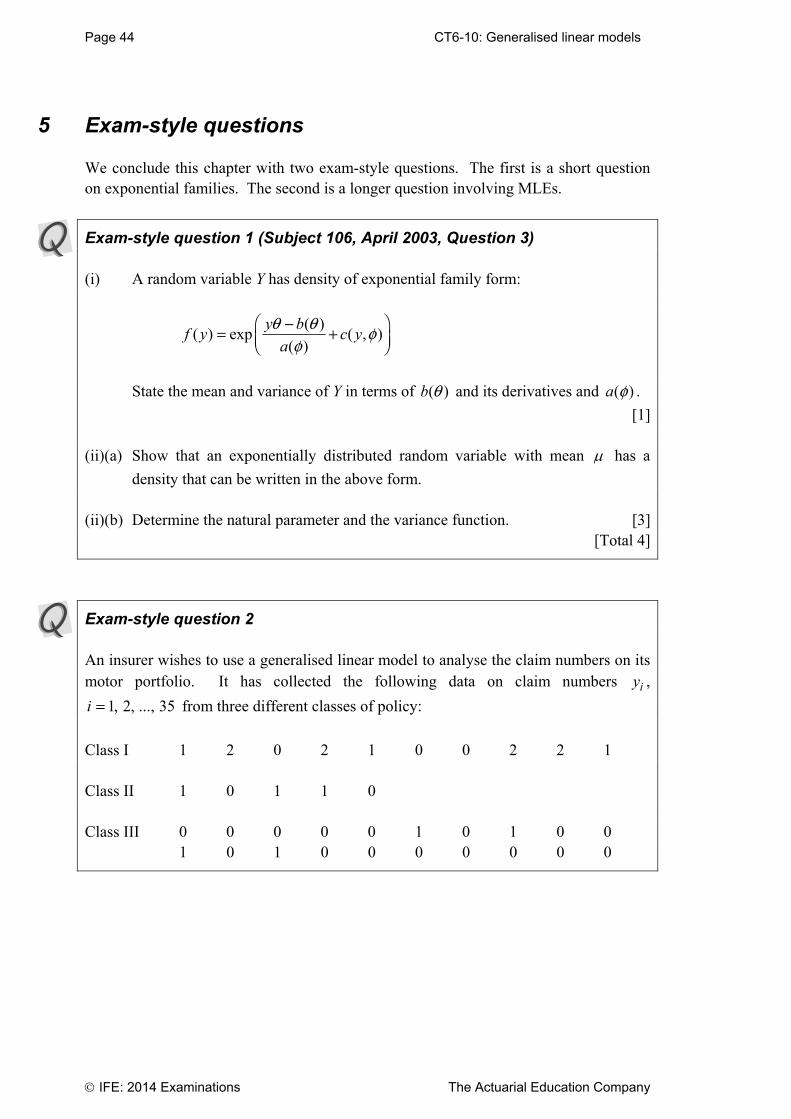
Page 44 CT6-10: Generalised linear models
IFE: 2014 Examinations The Actuarial Education Company
5 Exam-style questions
We conclude this chapter with two exam-style questions. The first is a short question on exponential families. The second is a longer question involving MLEs.
Exam-style question 1 (Subject 106, April 2003, Question 3) (i) A random variable Y has density of exponential family form:
( )
( ) exp ( , )( )
y bf y c y
a
q q ff
Ê ˆ-= +Á ˜Ë ¯
State the mean and variance of Y in terms of ( )b q and its derivatives and ( )a f .
[1] (ii)(a) Show that an exponentially distributed random variable with mean has a
density that can be written in the above form. (ii)(b) Determine the natural parameter and the variance function. [3] [Total 4]
Exam-style question 2 An insurer wishes to use a generalised linear model to analyse the claim numbers on its motor portfolio. It has collected the following data on claim numbers iy ,
1, 2, ..., 35i = from three different classes of policy:
Class I 1 2 0 2 1 0 0 2 2 1 Class II 1 0 1 1 0 Class III 0 0 0 0 0 1 0 1 0 0 1 0 1 0 0 0 0 0 0 0
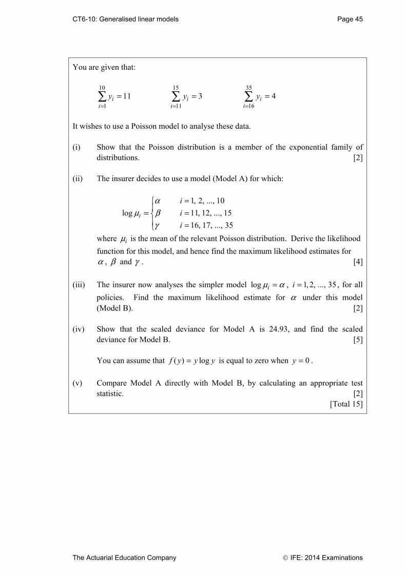
CT6-10: Generalised linear models Page 45
The Actuarial Education Company IFE: 2014 Examinations
You are given that:
10
1
11ii
y=
=Â 15
11
3ii
y=
=Â 35
16
4ii
y=
=Â
It wishes to use a Poisson model to analyse these data. (i) Show that the Poisson distribution is a member of the exponential family of
distributions. [2] (ii) The insurer decides to use a model (Model A) for which:
1, 2, ..., 10
log 11, 12, ..., 15
16, 17, ..., 35i
i
i
i
am b
g
=ÏÔ= =ÌÔ =Ó
where im is the mean of the relevant Poisson distribution. Derive the likelihood
function for this model, and hence find the maximum likelihood estimates for a , b and g . [4]
(iii) The insurer now analyses the simpler model log im a= , 1, 2, ..., 35i = , for all
policies. Find the maximum likelihood estimate for a under this model (Model B). [2]
(iv) Show that the scaled deviance for Model A is 24.93, and find the scaled
deviance for Model B. [5] You can assume that ( ) logf y y y= is equal to zero when 0y = .
(v) Compare Model A directly with Model B, by calculating an appropriate test
statistic. [2] [Total 15]

Page 46 CT6-10: Generalised linear models
IFE: 2014 Examinations The Actuarial Education Company
This page has been left blank so that you can keep the chapter summaries together as a revision tool.

CT6-10: Generalised linear models Page 47
The Actuarial Education Company IFE: 2014 Examinations
Chapter 10 Summary Exponential family There is a wide variety of distributions (normal, Poisson, binomial, gamma and exponential) that have a common form, called the exponential family. If the distribution of Y is a member of the exponential family then the density function of Y can be written in the form:
( ( ))( ; , ) exp ( , )
( )
È ˘-= +Í ˙Î ˚
Yy b
f y c ya
q qq j jj
where q is the natural parameter which is a function of the mean ( )E Ym = only of the
distribution, and j is a scale parameter. Where the distribution has two parameters
(such as the normal, gamma and binomial distributions), we can take j to be the
parameter other than the mean. Where the distribution has one parameter (such as the Poisson and exponential distributions), we can take 1j = . However, the
parameterisations are not unique. Simple linear modelling (or linear regression) In a simple linear model we are trying to find the relationship between a response variable iY and a covariate ix . The relationship is:
0 1i i iY x eb b= + +
where ie are independent and identically normally distributed random variables with
mean 0 and variance 2s . We estimate the parameters 0b and 1b using linear regression, ie minimising the sum
of the squared error terms. The formulae for doing this are on Page 24 of the Tables. Multiple regression and the normal linear model Multiple regression is an extension of the simple linear regression above except there can be more than one covariate. The error terms are still assumed to be i.i.d normal
random variables with mean 0 and variance 2s .

Page 48 CT6-10: Generalised linear models
IFE: 2014 Examinations The Actuarial Education Company
Generalised linear models (GLMs) A GLM takes multiple regression one step further by allowing the data to be non-normally distributed. Instead, we can use any of the distributions in the exponential family. A GLM consists of three components: 1) a distribution for the data (Poisson, exponential, gamma, normal or binomial) 2) a linear predictor (a function of the covariates that is linear in the parameters) 3) a link function (that links the mean of the response variable to the linear predictor). A key output of a particular GLM is an equation linking the mean m of the response
variable to the covariates. Maximum likelihood estimation can be used to estimate the values of the parameters in the linear predictor. Link functions For each underlying distribution there is one link function that appears more natural to use than any other, usually because it will result in values for m that are appropriate to
the distribution under consideration. This is called the canonical link function, which means the “accepted” link function. The canonical link functions are given on Page 27 of the Tables. They are equivalent to the natural parameter q from the exponential family formulation of the PDF. Covariates A variable is a type of covariate (eg age) whose real numerical value enters the linear predictor directly, and a factor is a type of covariate (eg sex) that takes categorical values to which we need to assign numerical values for the purpose of the linear predictor.

CT6-10: Generalised linear models Page 49
The Actuarial Education Company IFE: 2014 Examinations
Linear predictors Linear predictors are functions of the covariates. They are linear in the parameters and not necessarily in the covariates. The simplest linear predictor is that for the constant model: h a= , which is used if it is
thought that the mean of the response variable is the same for all risks. An interaction term is used in the predictor when two covariates are believed not to be independent. In other words, the effect of one covariate (eg the age of an individual) is thought to depend on the value of another covariate (eg whether the sex of an individual is male or female). The dot “.” notation is used to indicate an interaction, eg age.sex is the interactive term between age and sex. The star “*” notation is used to indicate the main effects as well as the interaction, eg: age*sex = age + sex + age.sex An interaction (dot) term never appears on its own. Saturated model The model that provides the perfect fit to the data is called the saturated model. The saturated model has as many parameters as data points. The fitted values ˆim are equal
to the observed values iy . The saturated model is not useful from a predictive point of
view, however it is a good benchmark against which to compare the fit of other models via the scaled deviance. Scaled deviance The scaled deviance (or likelihood ratio) is used to compare the fit of the saturated model with the fit of another model. The scaled deviance of Model 1 is defined as:
( )1 12 ln lnSSD L L= -
The poorer the fit of Model 1, the bigger the scaled deviance will be.
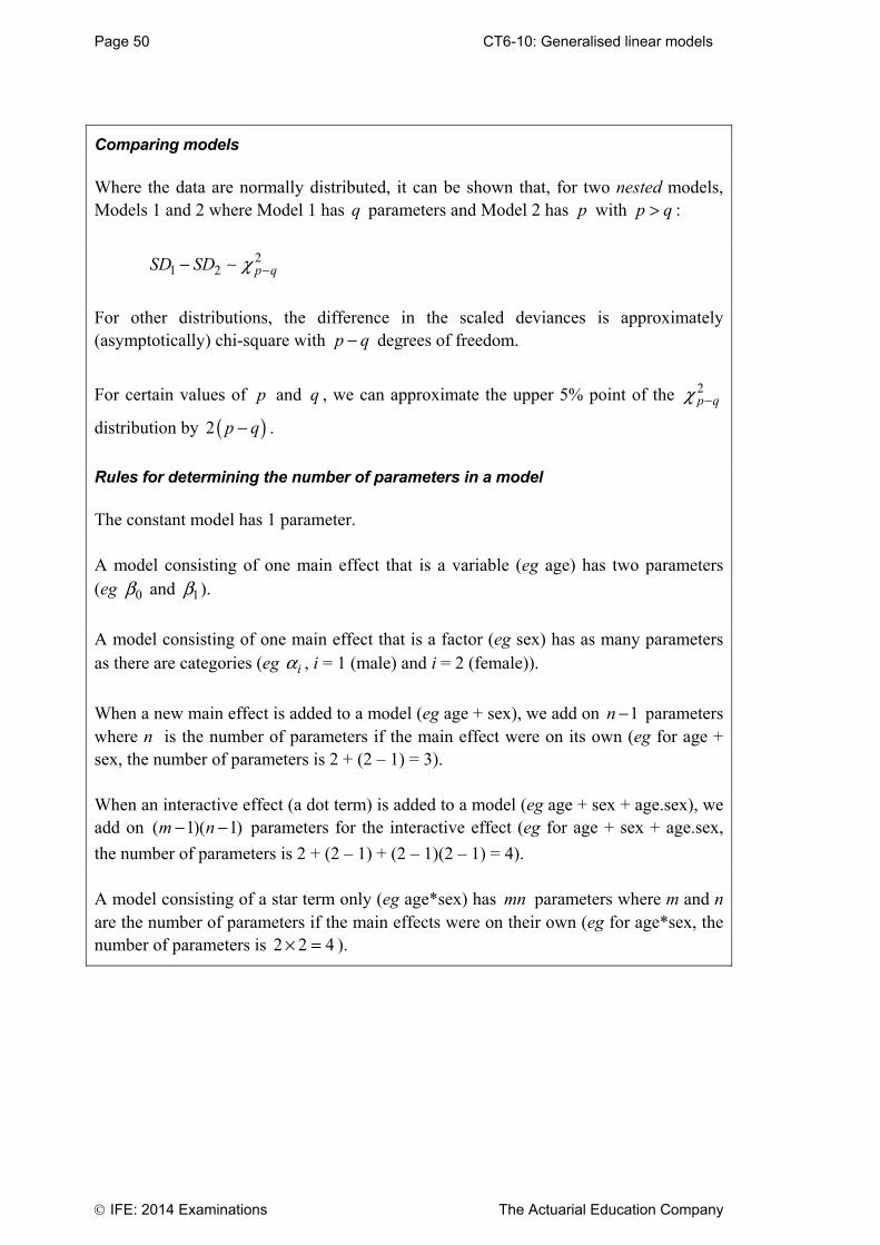
Page 50 CT6-10: Generalised linear models
IFE: 2014 Examinations The Actuarial Education Company
Comparing models Where the data are normally distributed, it can be shown that, for two nested models, Models 1 and 2 where Model 1 has q parameters and Model 2 has p with p q> :
21 2 p qSD SD c --
For other distributions, the difference in the scaled deviances is approximately (asymptotically) chi-square with p q- degrees of freedom.
For certain values of p and q , we can approximate the upper 5% point of the 2p qc -
distribution by ( )2 p q- .
Rules for determining the number of parameters in a model The constant model has 1 parameter. A model consisting of one main effect that is a variable (eg age) has two parameters (eg 0b and 1b ).
A model consisting of one main effect that is a factor (eg sex) has as many parameters as there are categories (eg ia , i = 1 (male) and i = 2 (female)).
When a new main effect is added to a model (eg age + sex), we add on 1n - parameters where n is the number of parameters if the main effect were on its own (eg for age + sex, the number of parameters is 2 + (2 – 1) = 3). When an interactive effect (a dot term) is added to a model (eg age + sex + age.sex), we add on ( 1)( 1)m n- - parameters for the interactive effect (eg for age + sex + age.sex,
the number of parameters is 2 + (2 – 1) + (2 – 1)(2 – 1) = 4). A model consisting of a star term only (eg age*sex) has mn parameters where m and n are the number of parameters if the main effects were on their own (eg for age*sex, the number of parameters is 2 2 4¥ = ).
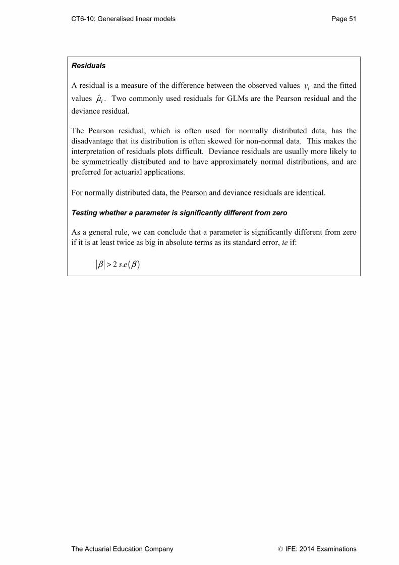
CT6-10: Generalised linear models Page 51
The Actuarial Education Company IFE: 2014 Examinations
Residuals
A residual is a measure of the difference between the observed values iy and the fitted
values ˆim . Two commonly used residuals for GLMs are the Pearson residual and the
deviance residual. The Pearson residual, which is often used for normally distributed data, has the disadvantage that its distribution is often skewed for non-normal data. This makes the interpretation of residuals plots difficult. Deviance residuals are usually more likely to be symmetrically distributed and to have approximately normal distributions, and are preferred for actuarial applications. For normally distributed data, the Pearson and deviance residuals are identical. Testing whether a parameter is significantly different from zero As a general rule, we can conclude that a parameter is significantly different from zero if it is at least twice as big in absolute terms as its standard error, ie if:
( )2 .s eb b>

Page 52 CT6-10: Generalised linear models
IFE: 2014 Examinations The Actuarial Education Company
Chapter 10 Formulae Exponential family form
( ( ))( ; , ) exp ( , )
( )
È ˘-= +Í ˙Î ˚
Yy b
f y c ya
q qq j jj
Mean, variance and variance function
( ) ( )= ¢E Y b q var( ) ( ) ( )= ¢¢Y a bj q ( ) ( )V bm q= ¢¢
The variance function is a function of the mean ( )E Ym = and gives a measure of how
( )var Y relates to m .
Scaled deviance
( )1 12 ln lnSSD L L= -
Chi-square test Models 1 has q parameters and Model 2 has p parameters with p q> . If Model 1 is a
sub model of Model 2 and the data are normally distributed then:
21 2 p qSD SD c --
For other distributions, the difference in the scaled deviances is approximately (asymptotically) chi-square with p q- degrees of freedom.
Pearson residual
This is ˆ
ˆvar( )
y mm
- where ( )ˆvar m is ( )var Y with any values of m replaced by their
fitted values m .
Deviance residual
This is ˆ( ) isign y dm- where 2id is the scaled deviance of the model.

CT6-10: Generalised linear models Page 53
The Actuarial Education Company IFE: 2014 Examinations
Chapter 10 Solutions Solution 10.1
Rating factors that might be used in the pricing of a single life annuity include:
age
sex (if permitted by legislation)
size of fund with which to purchase an annuity
postcode
health status (for impaired life annuities). Solution 10.2
The log likelihood function for a member of an exponential family is just:
( )( , ) ( , )
( )
-= +y bl c y
a
q qq f ff
Differentiating this with respect to q , we have:
( )
( )
- ¢=l y b
a
∂ q∂q f
Taking the expectation of this and setting the result to zero (ie applying the result we have just proved):
( ) ( )0
( )
- ¢ =E Y b
a
qf
Multiplying through by ( )a f gives the required result.
Now differentiating a second time:
2
2
( )
( )
- ¢¢=l b
a
∂ qf∂q

Page 54 CT6-10: Generalised linear models
IFE: 2014 Examinations The Actuarial Education Company
Using the second result proved above, we have:
2( ) ( )
0( ) ( )
È ˘Ê ˆ-¢¢ ¢Í ˙- + =Á ˜Ë ¯Í ˙Î ˚
b Y bE
a a
q qf f
The numerator of the second term is just the variance of Y , since we have already
shown that ( )¢b q is the mean. So multiplying through by ( ) 2È ˘Î ˚a f and rearranging, we
get:
var( ) ( ) ( )Y b a as required.
Solution 10.3
If we put 2=q m , we get the following expressions for the various functions:
( ) 2=a f f 2( ) / 4=b q q 2( , ) ½ ( / log 2 )= - +c y yf f pf
Using the formulae for the mean and variance, as before:
2 2( ) ( ) 2 / 4
4
¥= = = =¢E Y bmq q m
and 2var( ) ( ) ( ) 1/ 2 2= = ¥ = =¢¢Y b aq f f f s
So the mean and variance are m and 2s , as before.
Solution 10.4
Yes. Just as before with the normal distribution, there is more than one way to set up the parameters. However the natural approach is to use 1=f rather than 2=f , and
this is the approach you should use if you are asked to go through the algebra in the exam.
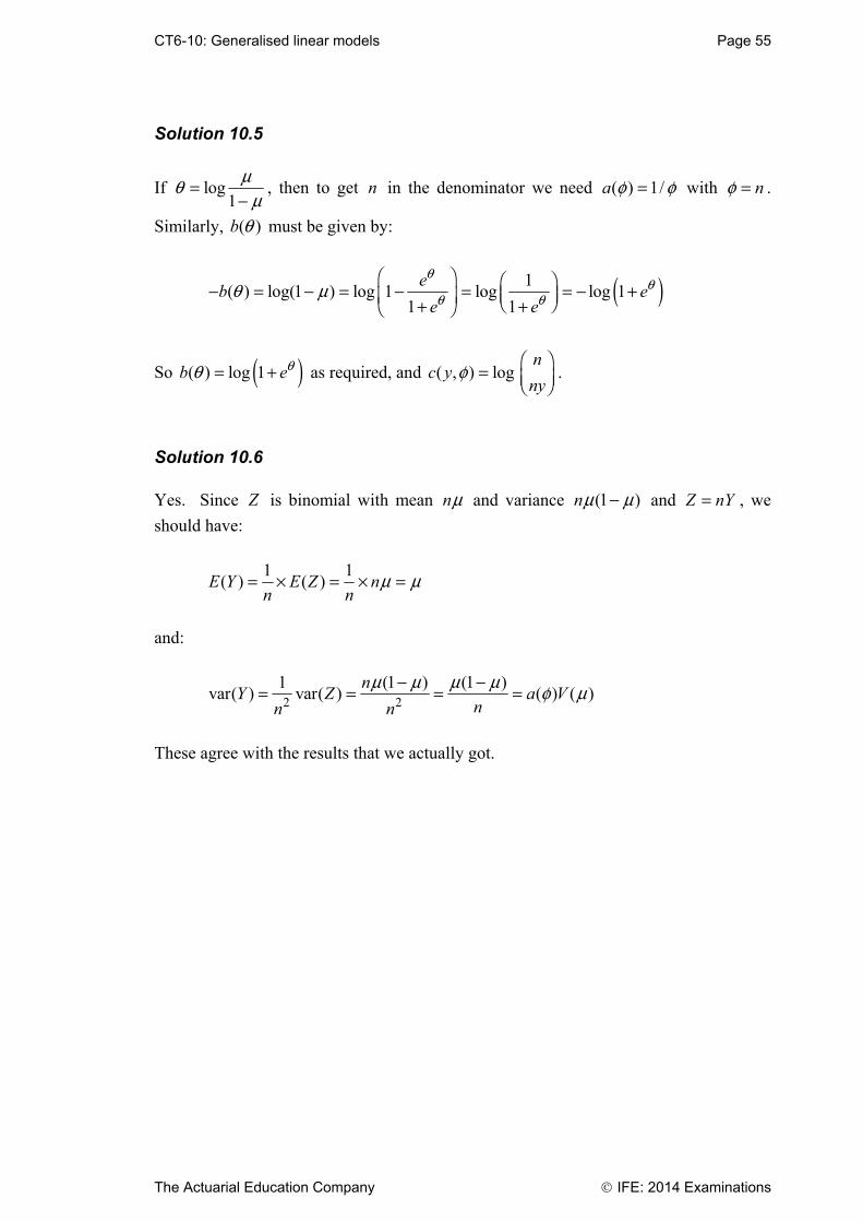
CT6-10: Generalised linear models Page 55
The Actuarial Education Company IFE: 2014 Examinations
Solution 10.5
If log1
=-mqm
, then to get n in the denominator we need ( ) 1/=a f f with = nf .
Similarly, ( )b q must be given by:
( )1( ) log(1 ) log 1 log log 1
1 1
Ê ˆ Ê ˆ- = - = - = = - +Á ˜Á ˜ Ë ¯+ +Ë ¯e
b ee e
q qq m
So ( )( ) log 1= +b eqq as required, and ( , ) logÊ ˆ
= Á ˜Ë ¯n
c yny
f .
Solution 10.6
Yes. Since Z is binomial with mean nm and variance (1 )-nm m and =Z nY , we
should have:
1 1
( ) ( )= ¥ = ¥ =E Y E Z nn n
m m
and:
2 2
1 (1 ) (1 )var( ) var( ) ( ) ( )
- -= = = =nY Z a V
nn n
m m m m f m
These agree with the results that we actually got.
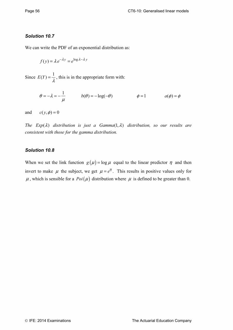
Page 56 CT6-10: Generalised linear models
IFE: 2014 Examinations The Actuarial Education Company
Solution 10.7
We can write the PDF of an exponential distribution as:
log( ) - -= =y yf y e el l ll
Since 1
( ) =E Yl
, this is in the appropriate form with:
1= - = -q lm
( ) log( )= - -b q q 1=f ( ) =a f f
and ( , ) 0=c y f
The ( )Exp l distribution is just a (1, )Gamma l distribution, so our results are
consistent with those for the gamma distribution. Solution 10.8
When we set the link function ( ) logg m m= equal to the linear predictor h and then
invert to make m the subject, we get ehm = . This results in positive values only for
m , which is sensible for a ( )Poi m distribution where m is defined to be greater than 0.

CT6-10: Generalised linear models Page 57
The Actuarial Education Company IFE: 2014 Examinations
Solution 10.9
(i) Using the values 3=N , 60=S and 1.501= -Ya , we get 1.6427=h , so that
0.83790=m . So the model predicts an 84% pass rate.
(ii) If the fourth assignment was submitted we use 4=N instead of 3=N and get
2.1886=h so that 0.8992=m . So the pass rate goes up by about 6%.
(iii) Using 3.196= -Na , 4=N and 100=S , we get 1.4976=h , so that
0.8172=m . So the highest possible pass rate for someone who does not attend
tutorials is about 82%. (iv) No. The minimum probability (for someone who does not attend tutorials or
submit assignments and who scores zero on the mock) is obtained from a value of 3.196= -h which gives a pass probability of about 4%. The maximum
probability of passing (for someone who goes to tutorials, submits all the assignments and scores 100% on the mock) comes from a value of 3.1926=h
which gives a pass rate of about 96%. So these are the maximum and minimum pass rates predicted by the model.
(v) In fact, what we are doing here is to find a parameter of a binomial distribution.
For any group of students with the same characteristics (ie all having the same values for all of the 3 factors), the number who pass may be well-modelled using a binomial distribution. The parameter of the binomial distribution
( ),Z Bin n m that we are trying to find is the value of 1
e
e
h
hm =+
that we found
above. Note that we are again using m to denote a probability as well as the mean of
the response variable /Y Z n= .
Page 58 CT6-10: Generalised linear models
IFE: 2014 Examinations The Actuarial Education Company
Solution 10.10
For this combination of factors we have: 12 1.5= + + =W Fh a b g
Using the link function given, we have:
1.5 4.48= =em
So the expected number of days unexplained absence in this case is about 4.5. Solution 10.11
We used this inverse function in the actuarial exam pass rates example. It is
( ) 111
1
ee
e e e
hh
h h hm--
-= = = ++ +
. It is an appropriate link function for the binomial
distribution since it results in values of m , the probability parameter, between 0 and 1.
Solution 10.12
A variable is a type of covariate (eg age) whose real numerical value enters the linear predictor directly, and a factor is a type of covariate (eg sex) that takes categorical values to which we need to assign numerical values for the purpose of the linear predictor. Solution 10.13
A helpful starting point is to consider the linear predictor for sex + vehicle group on its own. Summing the linear predictors for both of these main effects gives: i jh a b= +
Note that we don’t attempt to simplify this as ija for example, as this notation is
reserved for an interaction between sex and vehicle group, which we are not considering here.

CT6-10: Generalised linear models Page 59
The Actuarial Education Company IFE: 2014 Examinations
Now we consider the linear predictor for age * (sex + vehicle group). Recall that this can also be written as: age + (sex + vehicle group) + age . (sex + vehicle group) We sum the linear predictors for each of these three components:
( ) ( ) ( ) ( )0 1 0 1 .i j i jx xh g g a b g g a b= + + + + + +
Finally, we simplify by combining parameters: i j i jx xa b g d+ + +
Note that we have: combined 0g , ia and 0 . ig a into a new ia
left jb alone
combined 1g and 1 . ig a into ig
renamed 1 . jg b as jd .
Solution 10.14
The equations, which will be awkward to solve, are:
1 1 1 1 1
425 04 8 10 11 17a b a b a b a b a b
+ + + + - =+ + + + +
and: 4 8 10 11 17
5,028 04 8 10 11 17a b a b a b a b a b
+ + + + - =+ + + + +
Page 60 CT6-10: Generalised linear models
IFE: 2014 Examinations The Actuarial Education Company
Solution 10.15
If we write the PDF of the normal distribution in the form of an exponential family, we get:
2 2
2122 2
½( ) exp log 2
È ˘Ê ˆ-= - +Í ˙Á ˜Ë ¯Í ˙Î ˚
y yf y
q q pss s
So the log-likelihood function is:
2 221
22 21
2 22
21
2 22
21
22
1
½( , ) log 2
½ ½log 2
2
2log 2 ½
2
log 2 ½2
=
=
=
=
È ˘Ê ˆ-= - +Í ˙Á ˜Ë ¯Í ˙Î ˚
Ê ˆ- -= - + Á ˜
Ë ¯
Ê ˆ- += - - Á ˜Ë ¯
Ê ˆ-= - - Á ˜Ë ¯
Â
Â
Â
Â
ni i i i
i
ni i i i
i
ni i i i
i
ni i
i
y yl
y yn
y yn
yn
q qq f pss s
q qpss
q qpss
qpss
Alternatively we could start from the usual expression for the PDF of the normal distribution. Solution 10.16
Not in general. But the approximation is quite good for values of n between 5 and 15, and this is the range of values normally required in this type of calculation. Solution 10.17
The model that provides the perfect fit to the data is called the saturated model. The saturated model has as many parameters as data points. The fitted values ˆim are equal
to the observed values iy . The saturated model is not useful from a predictive point of
view; however it is a good benchmark against which to compare the fit of other models via the scaled deviance.
CT6-10: Generalised linear models Page 61
The Actuarial Education Company IFE: 2014 Examinations
Solution 10.18
For the improvement from Model 1 to Model pa, the decrease in the deviance is greater then twice the decrease in the degrees of freedom (81.13 2 7> ¥ ). So this suggests that Model pa is an improvement on Model 1. Similarly, 226.5 2 3> ¥ , so that using a model that takes account of car rating groups is again an improvement. Similarly, 204.1 2 3> ¥ , so that using a model that takes account of vehicle age is again an improvement. However, when we start to consider interactive effects, the degree of improvement in the model is much less. The decrease in the deviance is not greater than twice the decrease in the number of degrees of freedom. So there is little justification here for using a model that takes account of interactive effects. We would chose the model “pa + cg + va”. Solution 10.19
The expected truancy rates under the model are:
Expected number of unexplained absences in a year
Age
8 10 12 14
White Male 0.46 1.65 5.93 21.33
Female 0.35 1.25 4.48 16.12
Non-white Male 2.05 7.39 26.58 95.58
Female 1.55 5.58 20.09 72.24
So the differences are:
Differences
Age
8 10 12 14
White Male 1.34 0.35 0.37 –7.23
Female 0.15 0.35 0.52 0.08
Non-white Male 0.05 0.11 –1.08 –23.58
Female 1.25 0.62 –0.49 –4.04
Page 62 CT6-10: Generalised linear models
IFE: 2014 Examinations The Actuarial Education Company
Solution 10.20
If 2~ ( , )i iY N m s , then the Pearson residuals are -i iy ms
.
From Page 36, the scaled deviance is 2
21 1
( )
= =
- =Â Ân n
i ii
i i
yd
ms
. The deviance residuals are
given by:
( ) ( )- -- = - =i i i i
i i i i iy y
sign y d sign ym mm m
s s
Hence the Pearson residuals and the deviance residuals are the same. Solution to exam-style question 1 (Subject 106, April 2003, Question 3) (i) Mean and variance We have: [ ] ( )q= ¢E Y b var[ ] ( ) ( )Y a bf q= ¢¢
(ii)(a) Exponential form The PDF of the exponential distribution with mean m is:
1
( ) expm m
Ï ¸= -Ì ˝
Ó ˛
yf y
This can be written as an exponential:
1
( ) exp lnm m
Ï ¸= -Ì ˝
Ó ˛
yf y
Comparing this to the standard form given in part (i), we can define:
1 1
, ( ) 1, ( ) ln ln( ), ( , ) 0q f q q fm m
= - = = - = - - =a b c y
CT6-10: Generalised linear models Page 63
The Actuarial Education Company IFE: 2014 Examinations
(ii)(b) Natural parameter and variance function The natural parameter is q , so here the natural parameter is:
1
m-
The variance function is (by definition) ( )q¢¢b , so here we find:
22
1 1( ) ( )b b
Solution to exam-style question 2 (i) Exponential family For the Poisson distribution, we have:
( ) / !yf y e ymm-=
We wish to write this in the form:
( )
( ) exp ( , )( )
y bg y c y
a
q q ff
È ˘-= +Í ˙Î ˚
So, rearranging the Poisson formula:
log
( ) exp log !1
yf y y
m m-È ˘= -Í ˙Î ˚
We can see that this has the correct form if we write:
logq m= ( )b eqq m= = ( ) 1a f f= = ( , ) log !c y yf = -
Page 64 CT6-10: Generalised linear models
IFE: 2014 Examinations The Actuarial Education Company
(ii) Maximum likelihood estimates Using the rearranged form for the Poisson distribution from part (i), we see that the log of the likelihood function can be written:
log ( , , ) log log !I II III i i i iL y ym m m m m= - -Â Â Â (*)
This now becomes, for Model A:
10 15 35 35
1 11 16 1
log 10 5 20 log !i i i ii i i i
L y y y e e e ya b ga b g= = = =
= + + - - - -Â Â Â Â
35
1
11 3 4 10 5 20 log !ii
e e e ya b ga b g=
= + + - - - -Â (**)
Differentiating this log-likelihood function in turn with respect to a , b and g , we get:
log 11 10L eaa∂ = -∂
log 3 5L ebb∂ = -∂
and:
log 4 20L egg∂ = -∂
Setting each of these expressions equal to zero in turn, we find that: ˆ log1.1 0.09531a = =
ˆ log 0.6 0.51083b = = -
and: ˆ log 0.2 1.60944g = = -
These are our maximum likelihood estimates for a , b and g .
CT6-10: Generalised linear models Page 65
The Actuarial Education Company IFE: 2014 Examinations
(iii) Simpler model In this case the log-likelihood function reduces to:
35 35 35
1 1 1
log 35 log ! 18 35 log !i i ii i i
L y e y e ya aa a= = =
= - - = - -Â Â Â (***)
Differentiating this with respect to a , and setting the result equal to zero, we find that:
ˆ 18ˆ18 35 0 log 0.66498
35ea a Ê ˆ- = fi = = -Á ˜Ë ¯
(iv) Scaled deviance for Model A and Model B The scaled deviance for Model A is given by: 2(log log )S ASD L L= -
where log SL is the value of the log likelihood function for the saturated model, and
log AL is the value of the log-likelihood function for Model A.
For the saturated model, we replace the im ’s with the iy ’s in Equation (*) – as it fits
the observed data perfectly – so the expected results are the observed results. So:
log log log !
4 2 log 2 18 4log 2 4log 2 18 15.2274
S i i i iL y y y y= - -
= ¥ - - = - = -
  Â
We use the hint in the question here. logi iy y is zero when 0y = , and also when
1y = . So the only contribution to the first term is when 2y = , giving 4 lots of 2log 2 .
For the log likelihood for Model A, we replace the parameters a , b and g with their
estimates a , b and g in Equation (**):
35ˆˆ ˆ
1
ˆˆ ˆlog 11 3 4 10 5 20 log !
11log1.1 3log 0.6 4log 0.2 11 3 4 4log 2
27.6944
A ii
L e e e ya b ga b g=
= + + - - - -
= + + - - - -
= -
Â
Page 66 CT6-10: Generalised linear models
IFE: 2014 Examinations The Actuarial Education Company
The corresponding value for log AL without the final term is –24.9218.
So the scaled deviance is twice the difference in the log likelihoods:
( )2(log log ) 2 ( 15.2274) ( 27.6944) 24.93S ASD L L= - = - - - =
as required. We now repeat the process for Model B. Using Equation (***), the log likelihood for Model B is:
35ˆ
1
ˆlog 18 35 log !
1818log 18 4log 2 32.7422
35
B ii
L e yaa=
= - -
Ê ˆ= - - = -Á ˜Ë ¯
Â
The value without the final term is –29.9696. The scaled deviance is again twice the difference in the log likelihoods:
( )2(log log ) 2 ( 15.2274) ( 32.7422) 35.03S BSD L L= - = - - - =
(v) Comparing A with B We can use the chi-squared distribution to compare Model A with Model B. We calculate the difference in the scaled deviances (which is just 2(log log )A BL L- ):
35.03 24.93 10.10- = This should have a chi-squared distribution with 3 1 2- = degrees of freedom, which has a critical value at the upper 5% level of 5.991. Our value is significant here, since 10.10 5.991 , so that Model A is a significant improvement over Model B. We prefer Model A here.

CT6-11: Run-off triangles Page 43
The Actuarial Education Company IFE: 2014 Examinations
Chapter 11 Summary An important feature of the claims process in general insurance is reserving ie estimating the components of claims reserves, which include outstanding reported claims, IBNR, reopened claims and claims handling expenses. Run-off triangles (or delay triangles) provide a method of tabulating claims data and studying the underlying statistical model. Three methods used for projecting claims are the basic chain ladder method, the average cost per claim method and the Bornhuetter-Ferguson method. Basic chain-ladder – method Calculate development factors from the cumulative claims data.
Use these development factors to project the future cumulative claims. Basic chain-ladder – assumptions The first accident year is fully run off.
Claims in each development year are a constant proportion in monetary terms of total claims for each accident year.
Inflation is not allowed for explicitly, rather it is allowed for implicitly as a weighted average of past inflation.
Inflation-adjusted chain ladder – method Apply past inflation factors to incremental data so that all the claims data in the
table is expressed in the monetary terms of the most recent accident year.
Accumulate the data and calculate development factors.
Use these development factors to project the future cumulative claims (note that these will still be expressed in the monetary terms of the most recent accident year).
Disaccumulate the data to make it incremental.
Apply future inflation assumptions to convert the outstanding claim payments into the amounts relating to each future year.

Page 44 CT6-11: Run-off triangles
IFE: 2014 Examinations The Actuarial Education Company
Inflation-adjusted chain ladder – assumptions The first accident year is fully run off.
Claims in each development year are a constant proportion in real terms of total claims for each accident year.
Inflation is allowed for explicitly and we assume that both the past and future inflation assumptions are correct.
Average cost per claim – method Divide the entry in each cell in the cumulative claims table by the entry in the
corresponding cell of the claim number table. This gives the average cost per claim.
Calculate grossing-up factors for the average claim amounts. Use these to estimate the final average for each accident year.
Repeat the last step for the claim number table.
For each accident year, multiply together the figures from the ACPC and claim number tables.
Sum over all accident years to obtain the total projected loss estimate. Average cost per claim – assumptions The first accident year is fully run off.
The average cost per claim in each development year is a constant proportion in monetary terms of the ultimate average cost per claim for each accident year.
The number of claims in each development year is a constant proportion in of the ultimate number of claims for each accident year.
Inflation is not allowed for explicitly, rather it is allowed for implicitly as a weighted average of past inflation.
Bornhuetter-Ferguson – method Decide on the amount of the loss ratio.
Calculate development factors (as in BCL method).
Calculate the cumulative development factors f .

CT6-11: Run-off triangles Page 44a
The Actuarial Education Company IFE: 2014 Examinations
For each accident year that is not fully run-off: Multiply the earned premium by the loss ratio to obtain the initial estimate of the
ultimate loss
Use the initial estimate and the cumulative development factors to determine the expected amount paid out so far
Use this to see how much is expected to be paid in the future (emerging liability)
The revised estimate of the ultimate loss is the reported liability (last known figure) plus the emerging liability.
Finally: Sum the revised estimates of the ultimate losses for each accident year to obtain
an estimate of the total liability. Bornhuetter-Ferguson – assumptions The first accident year is fully run off.
The loss ratio is correct.
Claims in each development year are a constant proportion in monetary terms of total claims for each accident year.
Inflation is not allowed for explicitly, rather it is allowed for implicitly as a weighted average of past inflation.

Page 44b CT6-11: Run-off triangles
IFE: 2014 Examinations The Actuarial Education Company
Chapter 11 Formulae General statistical model Each entry, Cij , in the run-off triangle represents the incremental claims (as opposed to cumulative claims) and can be expressed in general terms as: Cij = rj . si . xi+j + eij where: rj is the development factor for year j, representing the proportion of claim payments in Development Year j. Each rj is independent of the Origin Year i. si is a parameter varying by Origin Year i representing the exposure, for example the number of claims (or claim amount) incurred in Origin Year i. xi+j is a parameter varying by calendar year, for example representing inflation. eij is an error term.

CT6-12: Time series 1 Page 57
The Actuarial Education Company IFE: 2014 Examinations
Chapter 12 Summary Univariate time series
A univariate time series is a sequence of observations tX recorded at regular
intervals. The state space is continuous but the time set is discrete. Such series may follow a pattern to some extent, for example possessing a trend or seasonal component, as well as having random factors. The aim is to construct a model to fit a set of past data in order to forecast future values of the series. Stationarity It is easier (more efficient) to construct a model if the time series is stationary. A time series is said to be stationary, or strictly stationary, if the joint distributions of
1 2, , ...,
nt t tX X X and 1 2, , ...,
nk t k t k tX X X+ + + are identical for all 1 2, , , nt t t and
1 2, , , nk t k t k t+ + + in J and all integers n. This means that the statistical properties of
the process remain unchanged as time elapses. For most cases of interest to us, it is enough for the time series to be weakly stationary.
This is the case if the time series has a constant mean ( )tE X , constant variance
( )var tX and covariance ( )cov ,t t kX X + depends only on the lag k .
We are also interested primarily in purely indeterministic processes. This means knowledge of the values 1 2, , , nX X X is progressively less useful at predicting the
value of NX as N Æ• .
We redefine the term “stationary” to mean weakly stationary and purely indeterministic.
Importantly, the time series consisting of a sequence of white noise terms te is
weakly stationary and purely indeterministic. White noise is defined as a sequence of uncorrelated random variables with zero mean. It follows that this series has constant mean and variance, and covariance that depends only on whether the lag is zero or non-zero. It is purely indeterministic due to its random nature.
Page 58 CT6-12: Time series 1
IFE: 2014 Examinations The Actuarial Education Company
A time series process X is stationary if we can write it as a convergent sum of white noise terms. It can be shown that this is equivalent to saying that the roots of the characteristic polynomial of the X terms are all greater than 1 in magnitude. For example, if the time series is defined by 1 1 1 1t t p t p t t q t qX X X e e ea a b b- - - -= + + + + + + then the
characteristic polynomial is given by ( ) 11 ppq l a l a l= - - - . To find the roots, we
set this equal to zero and solve. Invertibility A time series process X is invertible if we can write the white noise term te as a
convergent sum of the X terms. It can be shown that this is equivalent to saying that the roots of the characteristic polynomial of the e terms are all greater than 1 in magnitude. For example, if the time series is given by 1 1 1 1t t p t p t t q t qX X X e e ea a b b- - - -= + + + + + + then the
characteristic polynomial is given by ( ) 11 qqf l b l b l= + + + . To find the roots, we
set this equal to zero and solve. Invertibility is a desirable characteristic since it enables us to calculate the residual terms and hence analyse the goodness of fit of a particular model. Markov A time series process X has the Markov property if:
[ ]1 21 2| , , , , |
nt s s s n s t sP X a X x X x X x X x P X a X xÈ ˘= = = = = = = =Î ˚
for all times 1 2 ns s s s t< < < < < and all states 1, , , na x x of S.
In other words we can predict the future state (at time t) from the current state (at time s) alone.
CT6-12: Time series 1 Page 58a
The Actuarial Education Company IFE: 2014 Examinations
Backward shift and difference operators The backwards shift operator, B, is defined as follows: 1t tBX X -= and Bm m= where m is a constant.
The backward shift operator can be applied repeatedly so that kt t kB X X -= .
The difference operator, — , is defined as follows: 1t t tX X X -— = -
The difference operator can be applied repeatedly so that 1 11
k k kt t tX X X- -
-— = — -— .
Note that the difference operator and backward shift operator are linked by 1 B— = - . Integrated of order d
A time series process X is integrated of order d, denoted ( )I d if its dth difference is
stationary. So X is ( )0I if the process X itself is stationary, and X is ( )1I if X— is
stationary. Autocovariance, autocorrelation and partial autocorrelation functions
If a time series is stationary, then its covariance ( )cov ,t t kX X + depends only on the
lag k. In this case, we define the autocovariance function as ( )cov ,k t t kX Xg += and
the autocorrelation function as ( ),k t t kCorr X Xr += .
For purely indeterministic time series processes X (where the past values of X become less useful the further into the future we look), 0kr Æ as k Æ• .
The autocorrelation and autocovariance function are linked by the equation 0
kk
grg
= .
Another important characteristic of a stationary random process is the partial
autocorrelation function (PACF) : 1, 2,k kf = , defined as the conditional correlation
of t kX + with tX given 1 1, ,t t kX X+ + - . Important formulae for the partial
autocorrelation are given on page 40 of the Tables.
Page 58b CT6-12: Time series 1
IFE: 2014 Examinations The Actuarial Education Company
Moving average time series
A time series process X is said to be ( )MA q (or moving average of order q) if it can be
written as a weighted average of the past q white noise terms (plus a new white noise
term): 1 1b b- -= + + +t t t q t qX e e e (zero mean)
1 1m b b- -= + + + +t t t q t qX e e e (mean m )
Features of ( )MA q time series include:
always stationary (as a finite sum of white noise)
invertible if all the roots of the characteristic equation
( ) 11 0= + + + =qqf l b l b l are greater than 1 in magnitude
not Markov
rk cuts off for >k q
fk decays as Æ•k .
A time series process that is ( )1MA is defined by: 1t t tX e em b -= + + . It is invertible if
1b < . The autocorrelation function is given by: 0 1 21,
1
br rb
= =+
and 0kr = for
1k > .

CT6-12: Time series 1 Page 58c
The Actuarial Education Company IFE: 2014 Examinations
Autoregressive time series
A time series process X is said to be ( )AR p (or autoregressive of order p) if it
depends on the past p terms of the series (plus a new white noise term):
1 1a a- -= + + +t t p t p tX X X e (zero mean)
1 1( ) ( )m a m a m- -= + - + + - +t t p t p tX X X e (mean m )
Features of ( )AR p time series include:
stationary if all the roots of the characteristic equation
( ) 11 0= - - - =ppq l a l a l are greater than 1 in magnitude
always invertible
only Markov if 1p =
rk decays as Æ•k
fk cuts off for k p> .
A time series process that is ( )1AR is defined by: ( )1t t tX X em a m-= + - + . It is
stationary if 1a < . The autocorrelation function is given by: kkr a= for 0k ≥ .
A particular type of ( )1AR process is known as a random walk: 1t t tX X e-= + . A
random walk itself is not stationary but its difference 1t t t tX X X e-— = - = is
stationary. We can express an (1)AR process as both a finite summation and an infinite summation
(assuming an infinite history) of white noise terms:
1
00
tt j
t t jj
X X ea a-
-=
= + Â and 0
jt t j
j
X ea•
-=
= Â
From the infinite history equation, we can deduce that ( ) 0tE X = and, if | | 1a < then
2
2var( )
1tX
sa
=-
.

Page 58d CT6-12: Time series 1
IFE: 2014 Examinations The Actuarial Education Company
Autoregressive moving average time series
A time series process X is said to be ( ),ARMA p q (or autoregressive moving average
of order p, q) if it is the sum of an ( )AR p and an ( )MA q time series:
1 1
1 1
a ab b
- -
- -
= + + +
+ + +
t t p t p t
t q t q
X X X e
e e (zero mean)
1 1
1 1
( ) ( )m a m a mb b
- -
- -
= + - + + - +
+ + +
t t p t p t
t q t q
X X X e
e e (mean m )
Features of ( ),ARMA p q time series include:
stationary if all the roots of the characteristic equation
( ) 11 0= - - - =ppq l a l a l are greater than 1 in magnitude
invertible if all the roots of the characteristic equation
( ) 11 0= + + + =qqf l b l b l are greater than 1 in magnitude
only Markov if 1p = , 0q =
rk decays as Æ•k
fk decays as Æ•k .
A time series process that is ( )1,1ARMA is defined by:
1 1( )t t t tX X e em a m b- -= + - + + . It is stationary if 1a < and invertible if 1b < .
The autocorrelation function is given by: 0 1 2
(1 )( )1,
(1 2 )
ab a br rb ab
+ += =+ +
and
11
kkr a r-= for 1k > .
Autoregressive integrated moving average time series
A time series process X is said to be ( ), ,ARIMA p d q (or autoregressive integrated
moving average of order p, d, q) if the thd difference:
= —dt tY X is a stationary ( , )ARMA p q time series process.
CT6-13: Time series 2 Page 41
The Actuarial Education Company IFE: 2014 Examinations
Chapter 13 Summary Box-Jenkins methodology
The Box-Jenkins methodology gives us a way of fitting an ( ), ,ARIMA p d q time series
model to an actual data set. The method consists of the following steps:
removing trends from the data set
identifying a model from the ( ), ,ARIMA p d q class
estimating parameters
diagnostic checks
forecasting. Removing trends Time series data can be modelled efficiently only if stationary. In particular, any deterministic trends or cycles must be removed before applying the modelling procedure. There are various ways of doing this. In addition, a time series may still be non-stationary because it is integrated. In this case the time series must be differenced.
Let the set of observed values of the time series process be tx .
Linear trends in the data can be removed by:
least squares trend removal, ie we move forward with ˆˆt ty x a bt= - - where a
and b have been determined using linear regression
differencing, ie we move forward with 1t t t ty x x x -= — = - .
Seasonal trends in the data can be removed by:
seasonal differencing, eg if a monthly trend is observed, we move forward with
12t t ty x x -= -
method of moving averages (applying a filter), eg if a monthly trend is observed, we move forward with
( )6 5 1 1 5 61
0.5 0.512t t t t t t t ty x x x x x x x- - - + + += + + + + + + + +
Page 42 CT6-13: Time series 2
IFE: 2014 Examinations The Actuarial Education Company
method of seasonal means, eg if a monthly trend is observed, we move forward
with ˆt t ty x q= - where tq is defined as the appropriate sample seasonal mean
(eg if t is a January value then consider the sample mean of the January data) less the sample overall mean m .
It may be possible to remove other trends in the data via a transformation. For example,
if the tx values appear to have an exponential trend, we could apply the
transformation logt ty x= .
Fitting an ARIMA process – finding “d” The following principles can be used to choose the appropriate value of d. 1. If the sample autocorrelation function kr decays slowly to 0, this indicates that
there are still trends in the data and that the data should be differenced again.
2. Let 2ˆds denote the sample variance of the process dtx— , then d can be set to the
value which minimises 2ˆds .
Fitting an ARIMA process – finding “p” and “q”
If the underlying time series process is ( )MA q then we would expect the sample
autocorrelation function kr to cut off for k q> . It can also be shown that kr has the
following approximate distribution for k q> :
2
1
10, 1 2
q
k ii
r Nn
r=
Ê ˆÊ ˆ+Á ˜Á ˜
Ë ¯Ë ¯Â
We might conclude that kr cuts off for k q> if 95% of its values fall within the
confidence interval:
2 2
1 1
1 11.96 1 2 , 1.96 1 2
q q
i ii in n
r r= =
È ˘Ê ˆ Ê ˆÍ ˙- + + +Á ˜ Á ˜Í ˙Ë ¯ Ë ¯Î ˚
 Â
CT6-13: Time series 2 Page 42a
The Actuarial Education Company IFE: 2014 Examinations
If the underlying time series process is ( )AR p then we would expect the sample partial
autocorrelation function kf to cut off for k p> . It can also be shown that kf has the
following approximate asymptotic distribution:
1ˆ 0,k Nn
f Ê ˆÁ ˜Ë ¯
.
We might conclude that kf cuts off for k p> if 95% of its values fall within the
confidence interval:
1 1
1.96 , 1.96n n
È ˘- +Í ˙Î ˚
Otherwise, we look to fit an ( ),ARMA p q model. In practice, we might start with an
( )1,1ARMA model and then apply diagnostic tests on the residuals to see whether this is
an acceptable fit. If not, we would try adding more parameters. Akaike’s Information Criterion (AIC) states that we should only consider adding an extra parameter if this results in a reduction of the residual sum of squares by a factor of
at least 2 ne- . Note that the formula for the sample autocorrelation function kr (or alternatively ˆkr ) is
given on page 40 of the Tables. The sample partial autocorrelation can then be calculated using the formulae (also on page 40 of the Tables) but with kr replaced by
kr .
Parameter estimation Once we have identified p , d and q , we move forward with a time series of the form:
1 1 2 2 1 1 2 2t t t p t p t t t q t qX X X X e e e ea a a b b b- - - - - -= + + + + + + + +
The parameters, the alphas and betas can be estimated as follows:
least squares estimation (which is equivalent to MLE if the error terms can be assumed to be normally distributed)
method of moments, where we equate population autocorrelations kr with
sample autocorrelations kr .
Page 42b CT6-13: Time series 2
IFE: 2014 Examinations The Actuarial Education Company
The final parameter of the model is 2s , the variance of the te , which may be estimated
using:
2 2
1
1ˆ ˆn
tt p
en
s= +
= Â where te denotes the estimate of the residual at time t.
Diagnostic tests If the model chosen is a good fit to the data, we would expect the estimates of the
residuals te to show the characteristics of white noise (ie a set of uncorrelated
random variables with zero mean). Examples of diagnostic tests include:
checking that the graph of the te terms is patternless
the te terms appear to be close to zero
the turning point test: the number of points of inflexion in the graph of the te
terms should fall within the 95% confidence interval:
( )2 16 29 2 16 292 1.96 , ( 2) 1.96
3 90 3 90
N NN N
È ˘- -- - - +Í ˙Î ˚
the sample autocorrelation kr of the te terms is close to zero and has an
approximate 1
0,Nn
Ê ˆÁ ˜Ë ¯
distribution so that 95% of its values should fall within
the confidence interval 1 1
1.96 , 1.96n n
È ˘- +Í ˙Î ˚
the Ljung and Box “portmanteau” test: if the te terms are white noise then
they should be uncorrelated. The sample autocorrelation kr of the te terms
satisfies: 2
2
1
( 2)m
km
k
rn n
n kc
=+
-Â for each m . This is a one-sided test.
CT6-13: Time series 2 Page 42c
The Actuarial Education Company IFE: 2014 Examinations
Forecasting Future values of the time series can be forecast using k-step ahead forecasting. We use the notation ˆ ( )nx k to be the estimate of the expected value of +n kX (given the
observations up to nX ). To determine ˆ ( )nx k , we take our time series equation and:
replace all unknown parameters by their estimated values
replace the random variables 1,..., nX X by their observed values 1,..., nx x
replace the random variables 1 1,...,+ + -n n kX X by their forecast values
ˆ ˆ(1),..., ( 1)-n nx x k
replace the innovations 1,..., ne e by the residuals 1 ˆ,..., ne e
replace the random variables 1 1,...,+ + -n n ke e by 0 (their expectations).
An alternative to k-step ahead forecasting is exponential smoothing. We use the notation ˆ (1)nx to be the estimate of the expected value of 1nX + (given the observations
up to nX ).
21 2ˆ (1) (1 ) (1 )a a a- -È ˘= + - + - +Î ˚n n n nx x x x
This is a weighted average of the past values but there is less emphasis on older values. The parameter a is called the smoothing parameter. Rearrangements include:
1ˆ ˆ(1) (1 ) (1)a a -= + -n n nx x x or [ ]1 1ˆ ˆ ˆ(1) (1) (1)a- -= + -n n n nx x x x
Multivariate time series We can write a univariate time series in multivariate (or vector) form. For example, the time series 1 1 2 2 1t t t t tX X X e ea a b- - -= + + + can be written as
1 2
1 1 1
2 2 2
0 1 0
0 1 0 0 0 0
0 0 1 0 0 0
t t t
t t t
t t t
X X e
X X e
X X e
a a b
- - -
- - -
Ê ˆ Ê ˆ Ê ˆÊ ˆ Ê ˆÁ ˜ Á ˜ Á ˜Á ˜ Á ˜= +Á ˜ Á ˜ Á ˜Á ˜ Á ˜
Ë ¯ Ë ¯Ë ¯ Ë ¯ Ë ¯
ie 1t t tX AX Be-= +
Whilst there are more parameters involved, the advantage of the vector form is that it displays the Markov property.
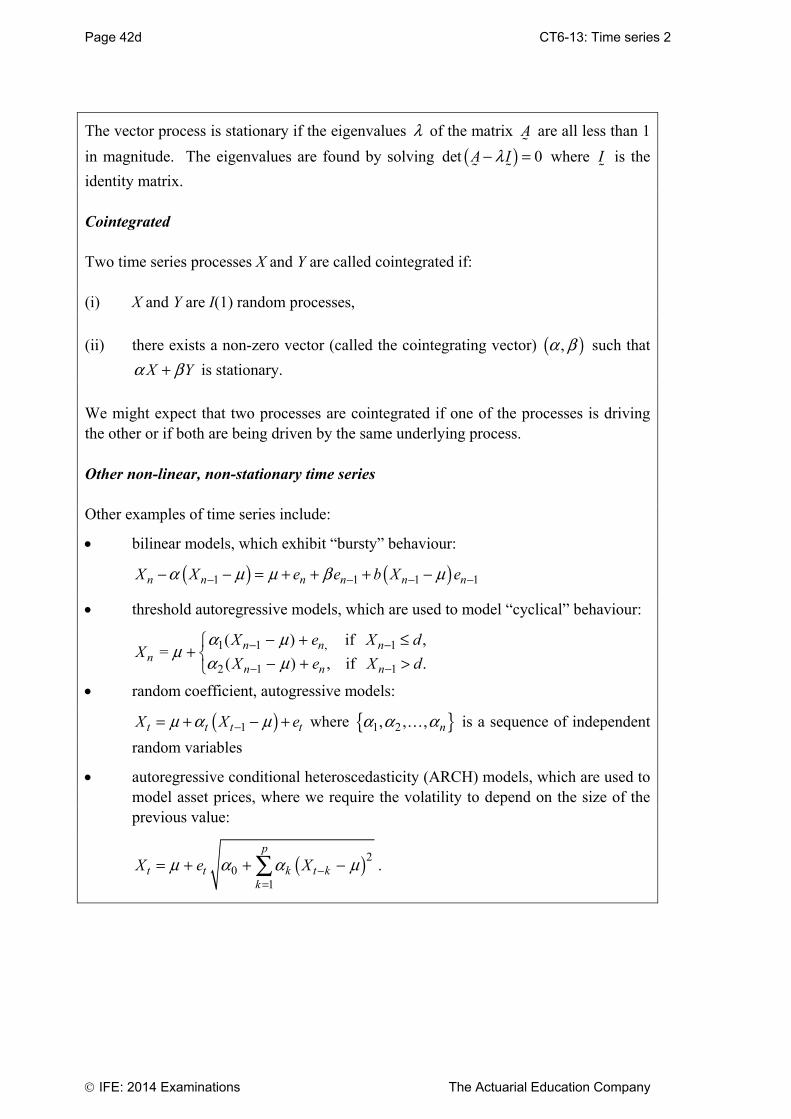
Page 42d CT6-13: Time series 2
IFE: 2014 Examinations The Actuarial Education Company
The vector process is stationary if the eigenvalues l of the matrix A
are all less than 1
in magnitude. The eigenvalues are found by solving ( )det 0A Il- =
where I
is the
identity matrix. Cointegrated Two time series processes X and Y are called cointegrated if: (i) X and Y are I(1) random processes,
(ii) there exists a non-zero vector (called the cointegrating vector) ( ),a b such that
X Ya b+ is stationary.
We might expect that two processes are cointegrated if one of the processes is driving the other or if both are being driven by the same underlying process. Other non-linear, non-stationary time series Other examples of time series include:
bilinear models, which exhibit “bursty” behaviour:
( ) ( )1 1 1 1n n n n n nX X e e b X ea m m b m- - - -- - = + + + -
threshold autoregressive models, which are used to model “cyclical” behaviour:
1 1 , 1
2 1 1
( ) if , =
( ) , if .n n n
nn n n
X e X dX
X e X d
a mm
a m- -
- -
- + £Ï+ Ì - + >Ó
random coefficient, autogressive models:
( )1t t t tX X em a m-= + - + where 1 2, , , na a a is a sequence of independent
random variables
autoregressive conditional heteroscedasticity (ARCH) models, which are used to model asset prices, where we require the volatility to depend on the size of the previous value:
( )201
p
t t k t kk
X e Xm a a m-=
= + + -Â .

CT6-14: Monte Carlo simulation Page 33
The Actuarial Education Company IFE: 2014 Examinations
Chapter 14 Summary Truly random vs pseudo-random numbers Truly random numbers can be generated by physical processes (eg dice, a roulette wheel or various electronic devices). Pseudo-random numbers are generated by a linear congruential generator (LCG). This generates random numbers using an initial integer value (a seed) and a recursive formula. The main advantages of pseudo-random numbers over truly random numbers are:
reproducibility
storage (only a seed and a single routine is needed)
efficiency (it is very quick to generate several billions of random numbers).
Reproducibility of the same set of random numbers is important if the random numbers are being used for:
sensitivity analysis
numerical evaluation of derivatives
comparative simulations, performance evaluation.
Monte-Carlo simulation One method of studying the statistical distribution of a stochastic quantity is to use a Monte Carlo method. This involves carrying out a large number of simulations of variates of a distribution, which can then be used to estimate probabilities and moments of the distribution. Monte Carlo methods are usually performed on a computer using pseudo-random numbers. Inverse transform method The inverse transform method can be used to generate random variates from
distributions using the CDF ( )F x .
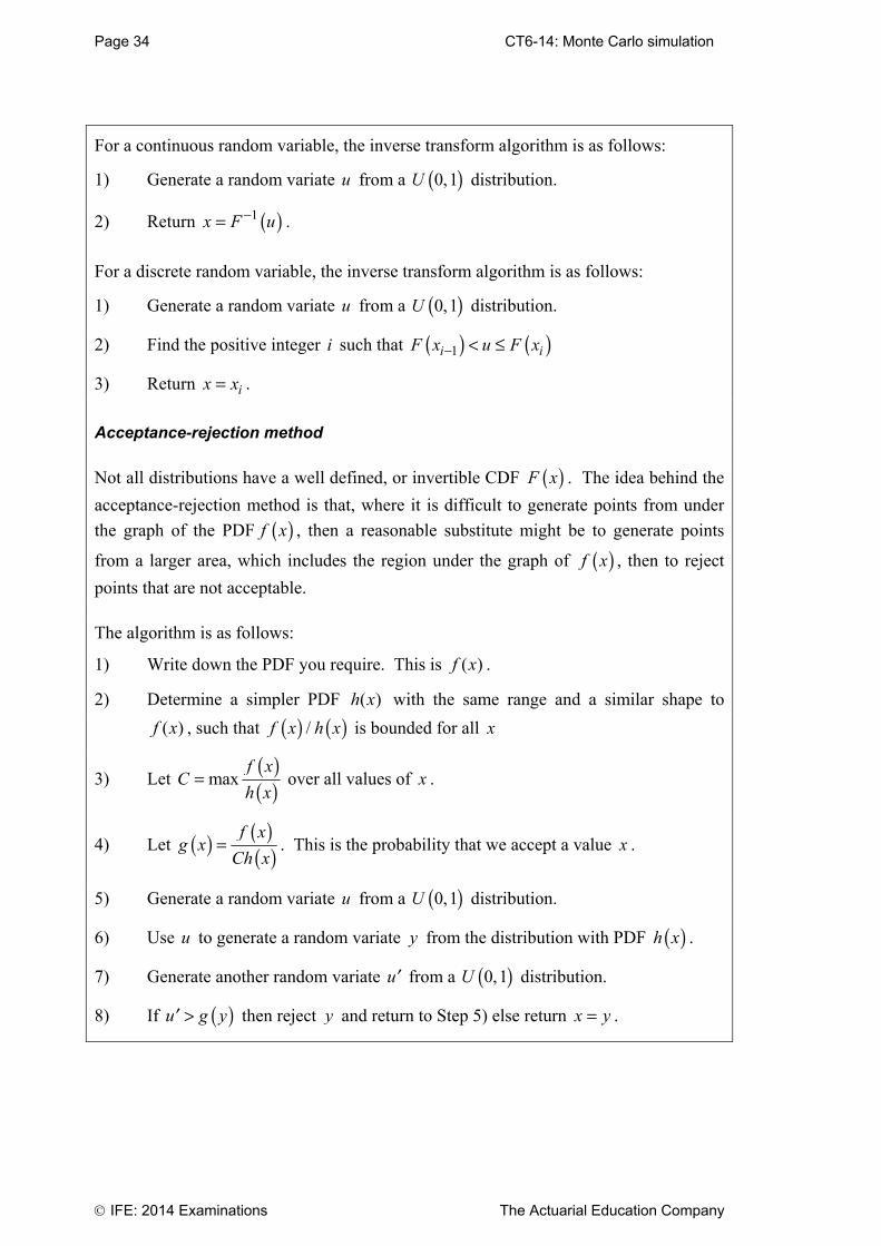
Page 34 CT6-14: Monte Carlo simulation
IFE: 2014 Examinations The Actuarial Education Company
For a continuous random variable, the inverse transform algorithm is as follows:
1) Generate a random variate u from a ( )0,1U distribution.
2) Return ( )1-=x F u .
For a discrete random variable, the inverse transform algorithm is as follows:
1) Generate a random variate u from a ( )0,1U distribution.
2) Find the positive integer i such that ( ) ( )1- < £i iF x u F x
3) Return = ix x .
Acceptance-rejection method
Not all distributions have a well defined, or invertible CDF ( )F x . The idea behind the
acceptance-rejection method is that, where it is difficult to generate points from under
the graph of the PDF ( )f x , then a reasonable substitute might be to generate points
from a larger area, which includes the region under the graph of ( )f x , then to reject
points that are not acceptable. The algorithm is as follows:
1) Write down the PDF you require. This is ( )f x .
2) Determine a simpler PDF ( )h x with the same range and a similar shape to
( )f x , such that ( ) ( )/f x h x is bounded for all x
3) Let ( )( )max=
f xC
h x over all values of x .
4) Let ( ) ( )( )=
f xg x
Ch x. This is the probability that we accept a value x .
5) Generate a random variate u from a ( )0,1U distribution.
6) Use u to generate a random variate y from the distribution with PDF ( )h x .
7) Generate another random variate ¢u from a ( )0,1U distribution.
8) If ( )>¢u g y then reject y and return to Step 5) else return =x y .
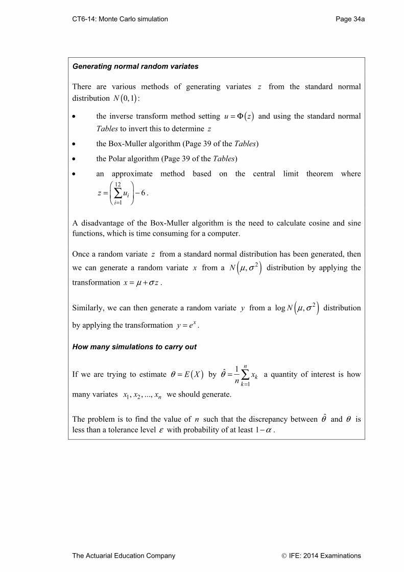
CT6-14: Monte Carlo simulation Page 34a
The Actuarial Education Company IFE: 2014 Examinations
Generating normal random variates There are various methods of generating variates z from the standard normal
distribution ( )0,1N :
the inverse transform method setting ( )= Fu z and using the standard normal
Tables to invert this to determine z
the Box-Muller algorithm (Page 39 of the Tables)
the Polar algorithm (Page 39 of the Tables)
an approximate method based on the central limit theorem where 12
1
6=
Ê ˆ= -Á ˜Ë ¯Â ii
z u .
A disadvantage of the Box-Muller algorithm is the need to calculate cosine and sine functions, which is time consuming for a computer. Once a random variate z from a standard normal distribution has been generated, then
we can generate a random variate x from a ( )2,N m s distribution by applying the
transformation = +x zm s .
Similarly, we can then generate a random variate y from a ( )2log ,N m s distribution
by applying the transformation = xy e .
How many simulations to carry out
If we are trying to estimate ( )= E Xq by 1
1ˆ
== Â
n
kk
xn
q a quantity of interest is how
many variates 1 2, , ..., nx x x we should generate.
The problem is to find the value of n such that the discrepancy between q and q is less than a tolerance level e with probability of at least 1-a .

Page 34b CT6-14: Monte Carlo simulation
IFE: 2014 Examinations The Actuarial Education Company
Where the discrepancy is measured by the absolute error ˆ -q q , we require:
( )ˆ 1- < ≥ -P q q e a
By the central limit theorem: ( )2ˆ 0, /- N nq q t .
Standardising, and approximating 2t by the sample variance 2t of the kx terms:
1ˆ ˆ/ /
-Ê ˆ< < ≥ -Á ˜Ë ¯P Z
n n
e e at t
Comparing with the upper and lower points /2za from the standard normal distribution,
we require that /2 ˆ /<z
na
et
and hence 2
2/2 2
ˆ>n za
te
.
Where the discrepancy is measured by the relative error ˆ /-q q q , we can show in a
similar way that we require: 2
2/2 2 2
ˆ>n za
te q
and use q to estimate q .