CSIS Discussion Paper No.125 (University of Tokyo)

Separating the Age Effect from a Repeat Sales Index:

Land and Structure Decomposition

SK Wong∗ , KW Chau† , K Karato‡ , C Shimizu§

December 10, 2013

Summary

Since real estate is heterogeneous and infrequently traded, the repeat sales model hasbecome a popular method to estimate a real estate price index. However, the modelfails to adjust for depreciation, as age and time between sales have an exact linearrelationship. This paper proposes a new method to estimate an age-adjusted repeatsales index by decomposing property value into land and structure components. Asdepreciation is more relevant to the structure than land, the property’s depreciation rateshould depend on the relative size of land and structure. The larger the land component,the lower is the depreciation rate of the property. Based on housing transactions datafrom Hong Kong and Tokyo, we find that Hong Kong has a higher depreciation rate(assuming a fixed structure-to-property value ratio), while the resulting age adjustmentis larger in Tokyo because its structure component has grown larger from the first tosecond sales.

1 Introduction

A price index aims to capture the price change of products free from any variations inquantity or quality. When it comes to real estate, the core problem is that it is heterogeneousand infrequently traded. Mean or median price indices are simple to compute, but propertiessold in one period may differ from those in another period. To overcome this problem, tworegression-based approaches are used to construct a constant-quality real estate price index(Shimizu et al. (2010)).

One is the hedonic price model, which specifies the property attributes to be controlledand uses time dummies to capture price changes over time. This method is often employedwhen data on property attributes are readily available, although omission of unobservedattributes or unique features of a property could lead to estimation bias. The other approachis the repeat sales model advanced by Bailey, Muth and Nourse (1963). It controls for

∗The University of Hong Kong†The University of Hong Kong‡University of Toyama§Correspondence: Chihiro Shimizu, Reitaku University & The University of British Columbia, Kashiwa,

Chiba 277-8686, Japan. E-mail: cshimizu@reitaku-u.ac.jp.

1

quality variations, including the uniqueness of each property, by tracking the price changeof properties that have been sold twice. This method is most useful when repeat sales areabundant.1

The repeat sales model is sometimes challenged for making a fundamentally incorrectassumption: quality could change over time even for the same property. For example, arepeat sales index may wrongly capture the price increase of a property due to the additionof a bedroom. But this is not the failure of the repeat sales model. If the change is known,the repeat sales model can be easily modified to account for it (Bailey, Muth and Nourse,1963, p.935). If the change is unknown, both the hedonic and repeat sales models wouldsuffer from the same problem. The real issue concerning the repeat sales model is that it isincapable of controlling for depreciation:

“Unfortunately, a depreciation adjustment cannot be readily estimated along with the priceindex using our regression method. . . Assuming that properties depreciate at a constant rateper unit time, . . . the x matrix [regressors] is singular. . . In applying our model, therefore,additional information would be needed in order to adjust the price index for depreciation.”(Bailey, Muth and Nourse, 1963, p.936).

Unlike any other quality change, the increase in age of a property is always identical to thetime elapsed between two sales. Including both age and time differences in the repeat salesregression gives rise to perfect collinearity. Not only are the age and time effects inseparable,but estimation also becomes impossible. Therefore, in many applications, the depreciationproblem is simply ignored, resulting in a repeat sales index that is biased downward.

Following Bailey, Muth and Nourse’s (1963) suggestion, several attempts were made to findthe “additional information” needed to solve the identification problem. Palmquist (1980)proposed a two-stage method: first obtain an independent estimate of the deprecation ratefrom the hedonic price model and then add it to back to the repeat sales index. Case andQuigley (1991), Hill, Knight, and Sirmans (1997), and Englund, Quigley and Redfearn (1998)offered a similar idea but combined the hedonic and repeat sales regressions into a hybridmodel for joint estimation. In both cases, cross-sectional differences in property age serve asthe additional information to identify the depreciation rate. Chau, Wong, and Yiu (2005)found another instrument to separate the age and time effects. They treated depreciationas a discounted cash flow problem and showed that for leasehold properties, the age effectvaries inversely with real interest rates. They also proved that simply converting the agevariable into dummies does not work. For instance, Cannaday, Munneke, and Yang (2005)had to drop two age dummies arbitrarily in order to avoid perfect collinearity, although ahigh degree of collinearity still remains.2

This paper proposes a new method to estimate an age-adjusted repeat sales index by

1Diewert(2007) summarized advantages and disadvantages in Repeat Sales measure and Hedonic mea-sure. And, Shimizu et al. (2010) compared Hedonic Index, Traditional Repeat Sales Index, Case-Shillertype Repeat Sales Index, Age adjusted Repeat Sales Index and new type Hedonic Index or Rolling WindowHedonic Index using Tokyo data..

2Shimizu, Nishimura and Watanabe(2010) and Karato, Movshuk and Shimizu (2010) also proposed newestimation method to separate the age and time effects. Karato, Movshuk and Shimizu (2010) tried toseparate age effect , time effect and cohort effect using semi -parametric approach; Generalized AdditiveModel or GAM.

2

decomposing property value into land and structure components.3 The key idea is thatdepreciation is more relevant to the structure than land. Since a property is the sum ofboth components, its depreciation rate depends on the relative size of land and structure.The larger the land component, the lower is the depreciation rate of the property. Section2 derives the relationship between the depreciation rate and a structure-to-property priceratio, and shows how the ratio can be used as additional information to separate the ageeffect from a repeat sales index. Moreover, similar to Chau, Wong, and Yiu (2005), the ageeffect is allowed to be non-linear by adopting a flexible functional form.

The proposed method is then used to estimate the repeat sales indices and depreciationrates for the housing markets in Hong Kong and Tokyo. While both are densely developedcities with high property prices, we expect them to have different deprecation patternsbecause the maintenance of condominiums (in particular the common areas) is a functionof the institutions governing the rights and duties of unit owners. Specifically, buildings inJapan have better upkeep in order to withstand earthquakes and fulfill the relevant legal(Building Standards Law) and insurance requirements. Section 3 will present the data andestimation results. Section 4 will further check the robustness of the estimates using a hybridand hedonic model. The last section is the conclusion.

2 An age-adjusted repeat sales model

Suppose property value (P ) is the sum of land value (L) and structure value (S).4 Thevalue of a new property is:

P (0) = L + S(0) (1)

where the number in brackets represents the building age. Aging reduces the value of thestructure value but not the land. Therefore, L is not a function of building age.

After A periods, the property reaches age A. Assuming a stable economy where L andS(0) remain unchanged, the property value will decline solely due to aging:

P (A) = L + S(0) × (1 −δ A) (2)

where δ is the depreciation rate of the structure. Equation 2 can be easily generalized toallow for a non-linear depreciation pattern. One way is to replace A with a more flexiblefunction g(A):

P (A) = L + S(0) × [1 −δ g(A)] (3)

3Diewert and de Haan (2011) and Diewert and Shimizu (2013) proposed a new hedonic model to decom-pose the Land and Structure component.

4Thorsnes (1997; 101) assumed that a related supply side model held instead of equation (2). He assumedthat housing was produced by a CES production function H(L, K) = [αLρ + βKρ]1/ρ where K is structurequantity and ρ ̸= 0; α > 0; β > 0 and α+β = 1. He assumed that property value V t

n is equal to ptH(Ltn, Kt

n)where pt,ρ , α and β are parameters to be estimated. However, Diewert’s builder’s model assumes that theproduction functions that produce structure space and that produce land are independent of each other.

3

Take g(A) = Aλ as an example. δ represents the initial depreciation rate of the structure.The depreciation rate would rise with age if λ>1, decrease with age if 0 < λ < 1, and remainat δ if λ = 1.

According to Equation 3, as long as land value is not zero, the property would depreciateat a rate lower than the structure. Specifically, the depreciation rate of P depends not onlyon δ but also on the ratio of new structure value to new property value:

(P (A) − P (0))/(P (0)) = −S(0)/P (0)δ g(A) (4)

Equation 4 has two important implications. First, given the same δ (e.g. building tech-nology) for all structures, properties in a high land value area would depreciate more slowlythan those in a low land value area. Second, even if the structure depreciates at a constantrate, the property’s depreciation rate is likely to be time-varying because structure and landvalues do not move at the same pace.5 The property would depreciate more (less) whenconstruction costs increase (decrease) faster than land costs.

The second implication provides us with a new perspective to resolve the perfect collinear-ity between age and time in the repeat sales method. This new perspective is different fromthe previous attempts that aimed to break down the linear relationship between age andtime by introducing “error” to the age variable. For instance, Cannaday, Munneke, andYang (2005) converted age into a set of dummy variables and dropped two such dummies toavoid perfect collinearity with time by making an arbitrary assumption that the depreciationrate is the same for certain ages. Our approach to the problem relies on the use of externalinformation to disentangle the effects of age and time. Chau, Wong, and Yiu (2005) alsofollowed this approach to derive the age effect as a function of real interest rates, but theirmodel is more applicable to leasehold interests. This paper proposes a more general frame-work to separate the age and time effects based on the relative size of land and structure.The ratio of new structure value to new property value is the external information we relyupon.

To motivate our age-adjusted repeat sales model, we can start with a hedonic price equa-tion and supplement it with the age term from Equation 4:

lnPit = Xiβ +αt −δ Rtg(Ait) + ϵit (5)

where Pit is the price of property i at time t; Xi is a vector of property attributes excludingbuilding age; β is a vector of the implicit price of the attributes; αt is the property priceindex at time t; and ϵit is a random error.

The third term on the right captures the age effect, where Rt is the ratio of constructioncost to new property price at time t. The smaller the Rt, the larger the non-depreciableland component, hence the smaller the age effect on property prices. This generalizes thestandard hedonic model, which assumes Rt = 1.

5In general, the inelastic supply of land makes land value more volatile and more sensitive to economicshocks than building value.

4

To allow for a non-linear depreciation pattern of the structure, the age function, g(Ait),adopts the Box-Cox transformation as shown in Equation 6.6 If λ = 1, the structuredepreciates at a constant rate δ. If λ > 1, the structure depreciates faster as its age increases.If λ < 1, the structure depreciates more slowly as its age increases. In all cases, δ is expectedto be positive.

g(Ait) =(

Aλit − 1λ

)(6)

Given that property i is sold twice at time s and t (where t > s) and there is no change inproperty attributes between the sales, our age-adjusted repeat sales model can be derivedfrom the (t − s)th difference of Equation 5:

ln(

Pit

Pis

)= (αt − αs) − δ [Rtg(Ait) − Rsg(Ais)] + (ϵit − ϵis) (7)

A key advantage of the repeat sales model is that it is less vulnerable to omitted variablebias – as long as the unobserved attributes do not change between sales, they will be cancelledout and do not affect estimation of the change in price index, αt − αs. Assuming ϵit − ϵis

is normally distributed, the parameters in Equation 7 can be estimated by the maximumlikelihood method. We call our new model in Equation 7 the “Age-R model”, which spellsout the key feature that building age is interacted with the structure-to-property value ratio.The traditional repeat sales model without the age term (called the BMN model) will alsobe estimated and compared against the Age-R model.

Again, if the Age-R model is correct, δ should be positive. Even if the structure depreciatesat a constant rate (i.e. λ = 1), the Age-R model is still free from perfect collinearity becausethe structure-to-property value ratio is unlikely to be fixed over time, especially upon thearrival of economic shocks. A time-varying structure-to-property value ratio indeed gives usa new angle to interpret the age effect. Consider a property of age 10 in 2012. For simplicity,let λ = 1, δ = 2%, and R2012=50%. Other things being equal, in 2013, aging by one yearshould depreciate the structure by 2% and the property by 1%. However, the structure-to-property value ratio may change. If R2013 is 60%, the property would actually depreciateby 1.2% – the greater depreciation was aquired as if the property had reached age 13 in oneyear. By contrast, if R2013 is 40%, the property would have looked as young as age 9, as theproperty would only depreciate by 0.8%. Therefore, the structure-to-property value ratioeffectively breaks the linear relationship between age and time differences between sales,making it possible to separate the age effect from a repeat-sales index.

6Box-Cox transformation requires that the age variable is strictly positive.

5

Table 1: Descriptive statistics of the repeat sales data in Hong Kong and TokyoHong Kong Island

Price at 1st sale Price at 2nd sale(HK$ million) (HK$ million)

Mean 4.0267 4.7299 63.32 81.72Std.Dev. 5.3257 6.9459 43.11 43.41Minimum 0.101 0.101 1 2Maximum 184.8 338 230 246N=190,890Tokyo

Price at 1st sale Price at 2nd sale¥10,000 ¥10,000

Mean 3,998.36 3,402.43 61.45 76.78Std.Dev. 3,180.38 2,582.23 34.73 36.86Minimum 34 9 1 2Maximum 80,000.00 68,000.00 192 201N=36,212

Age at 1st sale(quarters)

Age at 2nd sale(quarters)

Age at 1st sale(quarters)

Age at 2nd sale(quarters)

3 Estimated results of the age-adjusted repeat sales model

3.1 Data

Housing sales in Hong Kong and Tokyo are used to estimate the repeat sales propertyprice indices for the two cities. The time period runs from 1993Q1 to 2012Q2. 190,890pairs of repeat sales in Hong Kong Island were collected from the EPRC database, and36,212 pairs in the special 23 wards of Tokyo from a weekly magazine Shukan Jutaku Joho(Residential Information Weekly) published by Recruit Co., Ltd., which is one of the largestvendors of residential lettings information in Japan.7 Most of them are sales of condo units.The average sale price in Hong Kong is HK$4-5 million (US$600,000), whereas the averageprice in Tokyo is 30-40 million (US$400,000). The average building age in the repeat salessample is similar in both places: about 15 years old in the first sale and 20 years old in thesecond sale. The descriptive statistics of their sale prices and building ages are shown inTable 1.

An important variable for the age-R model is Rt, the ratio of construction cost to newproperty price. The average construction cost of a new residential building in Hong Kong isobtained from a major quantity surveying consultancy Rider Levett Bucknall (RLB), whichpublishes the RLB Hong Kong Cost Report every quarter. In Japan, the construction costis obtained from the Ministry of Land, Infrastructure, Transportation and Tourism (MLIT).

Estimating the price of new property is problematic. New properties constitute only asmall part of the existing stock and their prices can vary widely depending on their locationand developer. This means the use of new property prices could introduce a lot of noise to Rt.

7Recruit Co., Ltd. provided us with information on contract prices for about 24 percent of all listings.Using this information, we were able to confirm that prices in the final week were almost always identicalto the contract prices; see Shimizu et al. (2012).

6

Table 2: Maximum likelihood estimates of the age effect

Hong Kong Island Tokyo

δ 0.1029* 0.1035*λ 0.5547* 0.3212*

Log­likelihood ­19,185.82 11,097.23Note: * significant at the 1% level

We propose using the average property price in the entire housing market instead. Althoughthe average property price is a biased estimate of the new property price due to aging, thebias is likely to be stable as new properties will be added to and old properties removed fromthe existing stock. With a large sample of transactions in the existing stock, the averageage of transacted properties could remain more or less the same over time. Therefore, anyunderestimation from the use of all transacted properties could be compensated by a smallerδ in Equation 7. The model for estimating the age effect on property (rather than structure)is unaffected by this, but δ should be interpreted as a lower-bound estimate of the structure’sdepreciation rate.

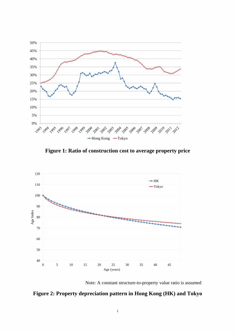
The ratio of construction cost to average property price is shown in Figure 1. As expected,the properties in Hong Kong and Tokyo have a larger portion for land than structure. Onaverage, the structure component only comprises 24% of the property value in Hong Kongand 37% in Tokyo. Note that these are upper-bound estimates because of the use of averageprices of all transacted properties instead of just new property prices.

3.2 Results of Age-R

The maximum likelihood estimates of the parameters δ and λ in Equation 7 are reportedin Table 2, whereas the price index results will be reported separately later. With Box-Coxtransformation, the marginal effect of age on log price is:

E[lnP (A)] = −δ RtA(λ−1) for A > 0 (8)

As expected, δ is positive and significant at the 1% level, confirming that the age effecton property price is negative. Moreover, the magnitude of δ in Hong Kong is almost thesame as that in Tokyo. At first sight, according to Equation 8, this can be interpreted asthat the structure shares a similar initial depreciation rate in both cities. But as mentionedbefore, the magnitude of δ could be biased downward due to the use of average price of alltransacted properties in estimating Rt.8 So, δ alone cannot tell if the two cities really havea similar initial depreciation rate at the structure level; rather, δ has to be combined withRt in order to compare the depreciation rates at the property level.

While the magnitude of δ appears to be large, it is only the initial depreciation rate. Sinceλ is smaller than 1 and significant, the depreciation pattern is confirmed to be non-linear:

8The downward bias in the δ estimate reinforces our prediction that the true δ should be positive.

7

the structure depreciates more slowly as its age increases. We can examine the depreciationpattern of property by considering δ and λ together. Assuming a property is worth $100 atage 1 and the ratio of construction cost to property price stays at its average level (Rt), theexpected price of property at age A is:

EP (A) = exp(ln P (1) − δRt

)(9)

Figure 2 plots the depreciation pattern calculated from Equation 9. Properties in Tokyodepreciate faster than those in Hong Kong initially, but the depreciation rate in Hong Kongpicks up soon and the rates reach a “break-even” at about Age 20. Over 50 years, propertyvalue has depreciated by 29% in Hong Kong and 26% in Tokyo – by that time, the propertyvalue is mostly derived from the land. The cumulative depreciation can be converted toan average annual depreciation rate of 0.58% and 0.52%, respectively. Bear in mind thatthese estimates are based on a constant structure-to-property value ratio. If the structurecomponent gets larger (smaller), the depreciation rate will go up (down) accordingly.

The higher average depreciation rate in Hong Kong could be caused by under-maintenanceof old buildings. In Hong Kong, the multiple ownership system for condominiums has createda lot of problemd in maintaining and managing the common areas (e.g. external walls,lifts, staircases, and lobbies). Court cases on building management issues and accidentsdue to building neglect are not uncommon. Legislation on mandatory building inspectionand maintenance did not exist until recently. In contrast, buildings in Japan are generallybetter maintained because they have to withstand earthquakes and fulfill the relevant legal(Building Standard Law) and insurance requirements.

The coefficients of the time dummies from the Age-R model in Equation 7 provide us withthe age-adjusted price indices for Hong Kong and Tokyo. As shown in Figures 3 and 4, ourage-R indices are above the BMN indices in both Hong Kong and Tokyo, suggesting thatproperty returns are higher after age adjustments. This result is intuitive, as the returncaptured by the BMN index is after depreciation.

Descriptive statistics of the indices are reported in Table 3. In Hong Kong, the meanreturn is 1.63% per quarter based on the age-R index and 1.56% based on the BMN index.The difference is 0.07% per quarter. In Tokyo, the mean return is -0.67% per quarter basedon the age-R index and -0.97% based on the BMN index. The difference is 0.30% perquarter. The age adjustment is larger for Tokyo than Hong Kong because Tokyo has alarger component of structure relative to land. Moreover, the structure-to-property valueratio in Tokyo is, on average, larger in the second sales than the first sales, whereas the ratioin Hong Kong is smaller in the second sales. This implies a bigger age adjustment for theTokyo housing market.

8

Table 3: Descriptive statistics of the BMN and Age-R indices

Hong Kong Island Tokyo

Age­R

 Mean return per quarter 1.63% ­0.67%

 Return volatility per quarter 5.26% 1.71%BMN Mean return per quarter 1.56% ­0.97% Return volatility per quarter 7.05% 2.18%Age adjustment in property return(per quarter) 0.07% 0.30%

Hybrid Mean return per quarter － ­0.53% Return volatility per quarter － 2.21%Hedonic Mean return per quarter － ­0.52% Return volatility per quarter － 2.06%Diffremces in property return  with Hybrid(per quarter) － ­0.14%

Diffremces in property return with Hedonic(per quarter) － ­0.15%

4 Comparison with other traditional models

4.1 Hybrid Model and Hedonic Model

Here, we will compare the new Age-R index with indices based on the hedonic and hybridmodels. As discussed in Introduction, the hedonic and hybrid models allow us to use a largerdataset comprising of both single and repeat sales, but they are more vulnerable to omittedvariable bias. Therefore, the purpose of this section is to check whether the three models –based on different assumptions and samples – will give similar estimates or not. If differentmethods share similar results, convergent validity is achieved. But it is not our purpose tojudge which model is right or wrong.

In the Tokyo data, there is sufficient attribute data (characteristics) about condominiumsto estimate a hedonic function. Thus, the hybrid method that was proposed to modify therepeat sales method proposed by Case and Quigley (1991) may also be applied. Here, toappraise the new Age-R proposed in the preceding section, we decided to compare the houseprice indices estimated by the hedonic method and the hybrid method using Tokyo data.

First, we will examine the hedonic model and hybrid model.Hill, Knight, and Sirmans (1997) distinguished the time effect and age effect by refining

Case and Quigley’s (1991) hybrid method (hedonic and repeat sales method joint modelestimation). The hedonic regression model is defined as:

9

yit = ln Pit + X′iβ + δAit + αt + ϵit (10)

where Pit is the price of property i at time t; Xi is a vector of property attributes excludingbuilding age; β is a vector of the implicit price of the attributes; is age effect; is i th propertyage at time t; αt is the fixed time effect at time t; and ϵit is a random error.

From sample i = 1, ..., N , let us take as a property that is transacted twice. The repeatsales regression model may be written as follows:

Yi = yit − yis = lnPit

Pis= τiδ + αt − αs + υi (i = 1, 2, ..., NR) (11)

Here,τi = Ait − Ais is the differential of the building age at time s and time t. If allsamples for (10) and (11) are pooled, the following regression model is obtained:

(y

Y

)=

(X A d

0 τ D

) β

δ

α

+

(ϵ

υ

)(12)

where d and D are the matrices of time dummy variables. A distinctive feature of thisapproach is that, by pooling a hedonic regression model and repeat sales regression model,the linear relationship between τi = Ait − Ais and D is disrupted and makes it possible toestimate simultaneously the age effect δ and time effect α.

The relationship between log price and the age term are linear in the hedonic equation ofthe hybrid model. To compare the age effects with the Box Cox transformed Age-R model,we estimate the hedonic regression model with the Box Cox transformed age term as follows:

ln Pit = X′iβ + δ

Aλit − 1λ

+ αt + ϵit (13)

4.2 Estimated results of Hybrid and Hedonic Model

Let us compare the data collected for the hedonic estimate in Tokyo wards with the dataused for estimation of repeat sales price (Table 4).

Although the number of repeat sales samples in the estimation period was 36,212, hedonicsamples increased to 375,374, or more than about 10 times. That is, by the repeat salesmethod, only 1/10 of the transactions that occurred from 1993 to the 2nd quarter of 2012could be utilized. If such a repeat sales sample is a typical random sample, it will besatisfactory, but if there is a bias in the sampling, there will be a bias in the index that isestimated.

First, looking at the average for prices, whereas this is 36,370,000 yen in the data for thehedonic model, in the repeat sales sample, the price of the first transaction is 39,980,000yen, and that of the second is 34,020,000 yen. In other words, the average for the hedonicsample is between the average for the first transaction and the average for the second trans-action. Looking at the number of post-construction years (A), whereas the average for the

10

Table 4: Descriptive statistics of the repeat sales data and hedonic data

Mean Std. Dev. Min Max

Hedonic Sample Price (\10,000) 3,637.92 2,684.75 185 112,000

Age (quarters) 68.45 41.93 0 352N=375,374

Repeat Sales Sample Price at 1st sale　(\10,000) 3,998.36 3,180.38 34 80,000

Price at 2nd sale　(\10,000) 3,402.43 2,582.23 9 68,000

Age at 1st sale　(quarters) 61.45 34.73 1 192

Age at 2nd sale　(quarters) 76.78 36.86 2 201N=36,212

hedonic sample is the 68th quarter, in the repeat sales sample, the average number of post-construction years for the first transaction was the 61st quarter, and for the second, it wasthe 76th quarter. Thus, similarly to prices, the average number of post-construction yearsis between the average for the first transaction and the average for the second transactions.This means that there is no significant bias in the repeat sales sample.

Using the hedonic database thus constructed, we estimated the hedonic function togetherwith the hybrid technique.

Here, comparing the aggregates for the hybrid model and the hedonic model based onTable 5, and comparing estimates, the coefficient for floor space is 1.098 for the hybridmethod and 1.091 for the hedonic method, so there is not much difference. As for distanceto the nearest station, this is -0.0071 by the hybrid method, and -0.009 by the hedonicmethod, whereas for times to the CBD (Center of the Business District), i.e., the time toTokyo Station, it is -0.0257 for the hybrid method and -0.006 for the hedonic method.

4.3 Comparison Age adjusted RS with traditional indexes

Figure 5 shows the estimated price index computed from the hybrid model and hedonicmodel, compared with BMN repeat sales price index and Age-R. The hybrid price indexand hedonic price index almost overlap; the new repeat sales price index (Age-R) follows asimilar trend but is less volatile. In particular, the BMN repeat sales price index is stronglybiased downwards, and by analogy, there is a depreciation bias that was clear from thisseries of studies. On the other hand, the Age-R proposed in this research, as comparedto the BMN repeat sales price index, is largely shifted so that it approximates the hedonicprice index and hybrid price index. As a result, the aggregation problem due to depreciationbias is largely improved. This result is extremely significant, although not as much as in thehybrid method.

However, even if we adjust for depreciation, a certain discrepancy remains between Age-R and the hedonic/hybrid price index. This discrepancy may be due to the fact that the

11

Table 5: Estimated results of Hedonic and Hybrid

Variable Coef. t ­value Coef. t ­value

Age (δ) ­0.0046 ­219.809 ­0.0192 ­72.135Box Cox (λ) － － 0.6353 182.680

Log (Floor Space) 1.1021 568.018 1.0890 1330.660Distance to Nearest Station ­0.0071 ­42.0458 ­0.0089 ­121.360

Distance to Tokyo Sta. ­0.0257 ­56.8187 ­0.0058 ­41.792Building Construction Dummy Yes

Ward Dummy Yes YesTime Dummies Yes Yes

const. 4.860 416.450 5.041 659.798

Number of obs. 108,969 375,374R­squared 0.998 0.889Adjusted R­squared 0.998 0.889S.E. of regression 0.189 0.182Log likelihood 26915.9 106200.0

samples were different or the choice of variables in the hedonic equation. In other words,although depreciation can be controlled for in both the Age-R and hedonic/hybrid models,the potential sample selection bias inherent in the repeat sales price method and the potentialomitted variable bias in the hedonic-based method cannot be resolved.

Moreover, if we compare the magnitudes of the depreciation bias and sample selectionbias, the bias due to depreciation is much larger. In other words, the Age-R evidentlyresolves the major part of the bias inherent in the repeat sales price method.

Next, Figure 6 compares the age indexes using aggregate parameters that correspond tothe number of post-construction years (A) estimated in the hybrid model, hedonic model,and the Age-R proposed in this research. Figure 7 and Table 6 show the marginal effects.

Table 6: Average depreciation rate

Age adjusted RS(HK)

Age adjusted RS(TKO)

Hedonic(TKO)

Hybrid(TKO)

over 50 yrs ­0.58% ­0.52% ­1.14% ­1.18%

over 40 yrs ­0.65% ­0.59% ­1.29% ­1.27%

0­10 yrs ­1.09% ­1.22% ­2.36% ­1.51%

10­20 yrs ­0.64% ­0.53% ­1.47% ­1.51%

20­30 yrs ­0.51% ­0.38% ­1.23% ­1.51%

30­40 yrs ­0.44% ­0.30% ­1.09% ­1.51%

40­50 yrs ­0.40% ­0.26% ­1.00% ­1.51%

12

As can be seen from Figure 1, the proportion accounted for by house construction costsin Japan was about 20% in 1991 during the country’s economic bubble years, but recentlyit increased to about 35%. Considering that the average between 1991-2012 is also about33%, it may be said that the average for 2012 is around the average level for the last 20years. In other words, considering there is no depreciation of land, regardless of how muchhouse prices have depreciated, the maximum value of this depreciation is 35%, and 65% ofthe price has been maintained.

Looking at Figure 6 from this assumption, the result estimated from the hybrid model andthe hedonic model is that 65% of house prices are factored in 15 years post-construction,and they will be at the 40% level at 50 years post-construction. This means, since landsuffers no depreciation, that the value of property is estimated to be negative. On the otherhand, looking at the result estimated from Age-R, the value at 50 years post-construction is70%, so that although it depreciates close to 65% that includes land values, a small propertyvalue remains.

From this result, it is clear that if we calculate the rate of depreciation by the hedonic orhybrid method taking land and property together, it will be largely over-estimated.

Comparing the marginal effects for depreciation (Figure 7, Table 6), in the 50 year-average,the rates of depreciation estimated from the hedonic method and hybrid method are abouttwice the rate of appreciation estimated from the new Age-R method proposed here, andthe discrepancy becomes larger, the larger the number of post-construction years.

In section 3, we suggested that property returns are higher after age adjustments.In addition to this analysis, we compared age R with hybrid and hedonic indexes in Tokyo.

The mean return of Age R is smaller than 0.14 and 0.15 % than that of Hybrid and Hedonicindexes(Table 3). Age R is overcoming depreciation problem in estimating Repeat Salesregression, while the returns from the hedonic and hybrid indexes are higher probably dueto the over-adjustment of depreciation as discussed above.

5 Conclusion

Since real estate is heterogeneous and infrequently traded, the repeat sales model hasbecome a popular method to estimate a property price indexes. However, the model fails toadjust for depreciation, as age and time between sales have an exact linear relationship. Thispaper proposes a new method to estimate an age-adjusted repeat sales index by decomposingproperty value into land and structure components. As depreciation is more relevant to thestructure than land, the property’s depreciation rate should depend on the relative size ofland and structure. The larger the land component, the lower the depreciation rate of theproperty. Based on housing transactions data from Hong Kong and Tokyo, Hong Konghas a higher depreciation rate (assuming a fixed structure-to-property value ratio), whilethe resulting age adjustment is larger in Tokyo because its structure component has grownlarger from the first to second sales.

To evaluate the Age-R proposed here, we input the Tokyo data into both the hybrid model

13

and the hedonic model, and then compared the estimated price indexes. This comparisonrevealed that newly proposed Age-R cancels out the inherent depreciation problem of therepeat sales model. Although the sample selection bias of the repeat sales model is expectedto remain, the magnitude of this problem was shown to be far smaller than that of the biasresulting from depreciation. We also compared the estimated depreciation rate here withthe depreciation rate estimated by using the hedonic model and hybrid model. Housingconsists of land and structure, but the depreciation that occurs only applies to the structure.When the hedonic model and hybrid model are used to estimate the depreciation rate of thecombined price of land and structure, the study revealed that as the structure value becomesnegative over a specified period of time, depreciation cuts into the land value. This was nota realistic result. Essentially, this result reiterates the importance of separating land andstructure when attempting to calculate the depreciation of housing, just as was proposed byDiewert and Shimizu (2013). Nevertheless, in regions where the repeat sales model, and notthe hedonic model, can be applied, the use of the Age-R is considered to be a valid methodfor calculating an appropriate depreciation rate.

In the “Handbook of Residential Property Indexes” that Eurostat began to distributein 2012,9 the hedonic model is recommended for estimating price indexes. However, whenattempting to estimate the real estate price index for the purpose of official statistics, therewill be many countries where the hedonic method cannot be applied due to existing restric-tions on data. This is because a variety of data about the characteristics of housing mustbe collected in order to apply the hedonic method. In these countries, the depreciation biaswill be a major problem when using the repeat sales model to estimate the price index. Thisfact is not only noted in the Eurostat handbook, but has also been made clear in this paper.

In conclusion, we believe that the new Age-R proposed in this paper is a valid means forsolving the problem of depreciation bias.

References

[1] Bailey, M. J., R. F. Muth, and H. O. Nourse. (1963). A Regression Model for RealEstate Price Index Construction, Journal of the American Statistical Association 58,933-942.

[2] Case, B and J. M. Quigley (1991), The dynamics of real estate prices, Review of Eco-nomics and Statistics 22, 50-58.

[3] Chau, K.W., S. K. Wong, and C. Y. Yiu (2005). Adjusting for Non-Linear Age Effects inthe Repeat Sales Index, Journal of Real Estate Finance and Economics 31:2, 137-153.

[4] Diewert, W. E (2007), The Paris OECD-IMF Workshop on Real Estate Price Indexes:Conclusions and Future Directions. Discussion Paper 07-01, Department of Economics,University of British Columbia, Vancouver, Canada, V6T1Z1.

9RPPI Handbook is available from the following website: http://epp.eurostat.ec.europa.eu/portal/page/portal/hicp/methodology/hps/rppi handbook

14

[5] Diewert, W.E., J. de Haan and R. Hendriks (2011). “Hedonic Regressions and the De-composition of a House Price index into Land and Structure Components,” DiscussionPaper 11-01, Department of Economics, University of British Columbia, Vancouver,Canada, V6T1Z1. Forthcoming in Econometric Reviews.

[6] Diewert, W. E. and C. Shimizu (2013). “A Conceptual Framework for CommercialProperty Price Indexes,” Discussion Paper 13-11, Vancouver School of Economics, Uni-versity of British Columbia.

[7] Englund, P., J. M. Quigley, and C. L. Redfearn (1998). Improved Price Indexes for RealEstate: Measuring the Course of Swedish Housing Prices, Journal of Urban Economics44, 171-196.

[8] Gatzlaff, D. H. and D. R. Haurin (1997). ”Sample Selection Bias and Repeat-SalesIndex Estimates,” Journal of Real Estate Finance and Economics, 14 (1), 33-50.

[9] Gatzlaff, D. H. and D. R. Haurin (1998). “Sample Selection and Biases in Local HouseValue Indices,” Journal of Urban Economics, 43(2), 199-222.

[10] Hill, R. C., J. R. Knight and C. F. Sirmans (1993) ”Estimation of Hedonic HousingPrice Models Using non Sample Information: A Montecarlo Study,” Journal of UrbanEconomics, 34(3), 319–346.

[11] Karato, K, O. Movshuk and C. Shimizu (2010). “Semiparametric Estimation of Time,Age and Cohort Effects in A Hedonic Model of House Prices,” Faculty of Economics,University of Toyama, Working Paper No. 25

[12] Palmquist, R. B (1980). Alternative Techniques for Developing Real Estate Price In-dexes, Review of Economics and Statistics 66, 394-404.

[13] Shimizu, C., K. G. Nishimura and T. Watanabe (2010). “House Prices in Tokyo -A Comparison of Repeat-sales and Hedonic Measures-,” Journal of Economics andStatistics, 230 (6), 792-813

[14] Shimizu, C., K.G. Nishimura and T. Watanabe (2012). “House Prices from Magazines,Realtors, and the Land Registry,” Property Market and Financial Stability, BIS PapersNo.64, Bank of International Settlements, March 2012, 29-38.

[15] Thorsnes, P. (1997). “Consistent Estimates of the Elasticity of Substitution betweenLand and Non-Land Inputs in the Production of Housing,” Journal of Urban Economics42, 98-108.

15

i  

Figure 1: Ratio of construction cost to average property price

Note: A constant structure-to-property value ratio is assumed

Figure 2: Property depreciation pattern in Hong Kong (HK) and Tokyo

0%

5%

10%

15%

20%

25%

30%

35%

40%

45%

50%

Hong Kong Tokyo

40

50

60

70

80

90

100

110

120

0 5 10 15 20 25 30 35 40 45

Age

Ind

ex

Age (years)

HK

Tokyo

ii  

Figure 3: Hong Kong Island’s repeat sales indices

BMN is the traditional repeat sales index; Age-R is the age-adjusted repeat sales index based on Equation 7

Figure 4: Tokyo’s repeat sales indices

0

0.5

1

1.5

2

2.5

3

3.5

BMN Age-R

0

0.2

0.4

0.6

0.8

1

1.2

BMN Age-R

iii  

Figure 5: Comparison of BMN, Age-R, Hedonic and Hybrid property price indexes in Tokyo

0.4

0.5

0.6

0.7

0.8

0.9

1.0

1.1

BMN Age-R

Hybrid Hedonic

iv  

Figure 6: Comparison of Age-R, Hedonic and Hybrid Age indexes

Figure 7: Marginal effect of depreciation rate

0

20

40

60

80

100

120

0 5 10 15 20 25 30 35 40 45

Age

Ind

ex

Age (year)

Age-R .

Hybrid .

Hedonic .

-2.0%

-1.8%

-1.6%

-1.4%

-1.2%

-1.0%

-0.8%

-0.6%

-0.4%

-0.2%

0.0%

0 5 10 15 20 25 30 35 40 45

Mar

gina

l Eff

ect

Age (year)

Age-R(HK) .

Age-R(Tokyo) .

Hybrid(Tokyo) .

Hedonic(Tokyo) .

v  

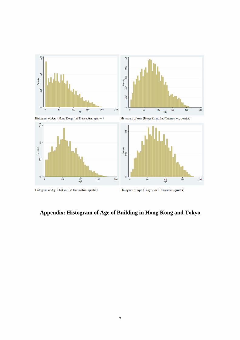
Appendix: Histogram of Age of Building in Hong Kong and Tokyo