CSE332: Data Abstractions

Lecture 21: Parallel Prefix and Parallel Sorting

Tyler RobisonSummer 2010

1

2

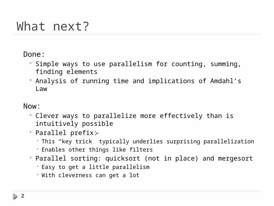
What next?

Done: Simple ways to use parallelism for counting, summing,

finding elements Analysis of running time and implications of Amdahl’s Law

Now: Clever ways to parallelize more effectively than is

intuitively possible Parallel prefix:

This “key trick” typically underlies surprising parallelization Enables other things like filters

Parallel sorting: quicksort (not in place) and mergesort Easy to get a little parallelism With cleverness can get a lot

3

The prefix-sum problemGiven int[] input, produce int[] output where output[i] is

the sum of input[0]+input[1]+…input[i]

Sequential is easy enough for a CSE142 exam:int[] prefix_sum(int[] input){ int[] output = new int[input.length]; output[0] = input[0]; for(int i=1; i < input.length; i++) output[i] = output[i-1]+input[i]; return output;}

This does not appear to be parallelizable; each cell depends on previous cell– Work: O(n), Span: O(n)– This algorithm is sequential, but we can design a

different algorithm with parallelism for the same problem

inout

6 4 16 10 16 14 2 86 10 26 36 52 66 68 76

4

The Parallel Prefix-Sum AlgorithmThe parallel-prefix algorithm has O(n) work but a span of

2log n So span is O(log n) and parallelism is n/log n, an

exponential speedup just like array summing

The 2 is because there will be two “passes” on the tree – more later

Historical note / local bragging: Original algorithm due to R. Ladner and M. Fischer in 1977 Richard Ladner joined the UW faculty in 1971 and hasn’t left

1968? 1973? recent

5

input

output

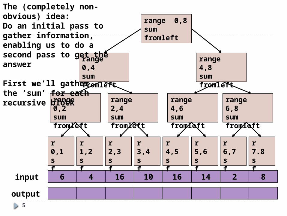
6 4 16 10 16 14 2 8

range 0,8sumfromleft

range 0,4sumfromleft

range 4,8sumfromleft

range 6,8sumfromleft

range 4,6sumfromleft

range 2,4sumfromleft

range 0,2sumfromleft

r 0,1s f

r 1,2s f

r 2,3s f

r 3,4s f

r 4,5s f

r 5,6s f

r 6,7s f

r 7.8s f

The (completely non-obvious) idea:Do an initial pass to gather information, enabling us to do a second pass to get the answer

First we’ll gather the ‘sum’ for each recursive block

6

First pass

input

output

6 4 16 10 16 14 2 8

range 0,8sumfromleft

range 0,4sumfromleft

range 4,8sumfromleft

range 6,8sumfromleft

range 4,6sumfromleft

range 2,4sumfromleft

range 0,2sumfromleft

r 0,1s f

r 1,2s f

r 2,3s f

r 3,4s f

r 4,5s f

r 5,6s f

r 6,7s f

r 7.8s f

6 4 16 10 16 14 2 8

10 26 30 10

36 40

76

For each node, get the sum of all values in its range; propagate sum up from leaves

Will work like parallel sum, but recording intermediate information

7

Second pass

input

output

6 4 16 10 16 14 2 8

6 10 26 36 52 66 68 76

range 0,8sumfromleft

range 0,4sumfromleft

range 4,8sumfromleft

range 6,8sumfromleft

range 4,6sumfromleft

range 2,4sumfromleft

range 0,2sumfromleft

r 0,1s f

r 1,2s f

r 2,3s f

r 3,4s f

r 4,5s f

r 5,6s f

r 6,7s f

r 7.8s f

6 4 16 10 16 14 2 8

10 26 30 10

36 40

760

0

0

0

36

10 36 666 26

52 68

10 66

36

Using ‘sum’, get the sum of everything to the left of this range (call it ‘fromleft’); propagate down from root

8

The algorithm, part 1

1. Propagate ‘sum’ up: Build a binary tree where Root has sum of input[0]..input[n-1] Each node has sum of input[lo]..input[hi-1]

Build up from leaves; parent.sum=left.sum+right.sum A leaf’s sum is just it’s value; input[i]

This is an easy fork-join computation: combine results by actually building a binary tree with all the sums of ranges Tree built bottom-up in parallel Could be more clever; ex: heap-like ‘array as tree’

representation

Analysis of this step: O(n) work, O(log n) span

9

The algorithm, part 2

2. Propagate ‘fromleft’ down: Root given a fromLeft of 0 Node takes its fromLeft value and

Passes its left child the same fromLeft Passes its right child its fromLeft plus its left child’s sum (as

stored in part 1) At the leaf for array position i,

output[i]=fromLeft+input[i]

This is another fork-join computation: traverse the tree built in step 1 and assign to output at leaves (don’t return a result)

Analysis of this step: O(n) work, O(log n) spanTotal for algorithm: O(n) work, O(log n) span

10

Sequential cut-offAdding a sequential cut-off isn’t too bad:

Step One: Propagating Up: Sequentially compute sum for rangeThe tree itself will be shallower

Step Two: Propagating Down: output[lo] = fromLeft + input[lo];

for(i=lo+1; i < hi; i++)

output[i] = output[i-1] + input[i]

11

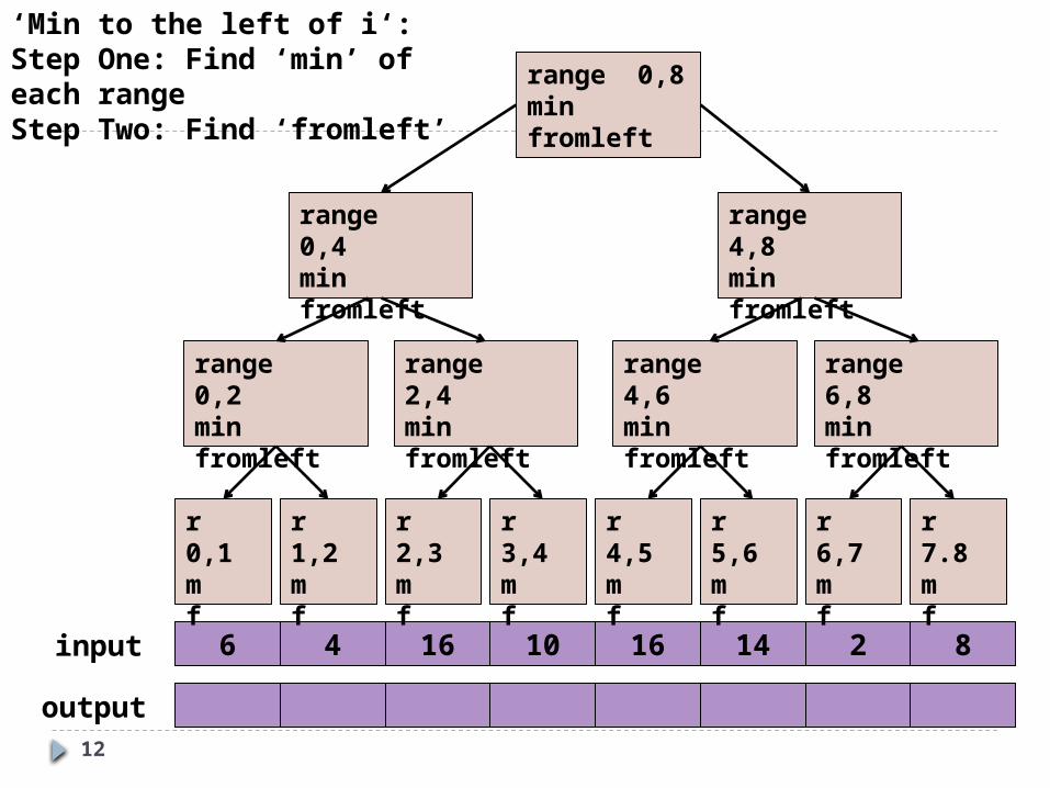
Parallel prefix, generalizedJust as sum-array was the simplest example of a

pattern that matches many problems, so is prefix-sum

Array that stores minimum/maximum of all elements to the left of i, for any i

Is there an element to the left of i satisfying some property?

Count of all elements to the left of i satisfying some property

We did an inclusive sum, but exclusive is just as easy

12

input

output

6 4 16 10 16 14 2 8

range 0,8minfromleft

range 0,4minfromleft

range 4,8minfromleft

range 6,8minfromleft

range 4,6minfromleft

range 2,4minfromleft

range 0,2minfromleft

r 0,1m f

r 1,2m f

r 2,3m f

r 3,4m f

r 4,5m f

r 5,6m f

r 6,7m f

r 7.8m f

‘Min to the left of i‘: Step One: Find ‘min’ of each rangeStep Two: Find ‘fromleft’

13

Filter[Non-standard terminology]

Given an array input, produce an array output containing only elements such that f(elt) is true

Example: input [17, 4, 6, 8, 11, 5, 13, 19, 0, 24]

f: is elt > 10

output [17, 11, 13, 19, 24]

Looks hard to parallelize Determining whether an element belongs in the output is

easy But getting them in the right place in the output is hard;

seems to depend on previous results

14

Parallel prefix to the rescue

1. Use a parallel map to compute a bit-vector for true elementsinput [17, 4, 6, 8, 11, 5, 13, 19, 0, 24]

bits [1, 0, 0, 0, 1, 0, 1, 1, 0, 1]

2. Do parallel-prefix sum on the bit-vectorbitsum [1, 1, 1, 1, 2, 2, 3, 4, 4, 5]

3. Allocate an output array with size bitsum[input.length-1]

4. Use a parallel map on input; if element i passes test, put it in output at index bitsum[i]-1Result: output [17, 11, 13, 19, 24]

output = new array of size bitsum[n-1]if(bitsum[0]==1) output[0] = input[0];FORALL(i=1; i < input.length; i++) if(bitsum[i] > bitsum[i-1]) output[bitsum[i]-1] = input[i];

Filter: elt > 10

15

Filter comments

First two steps can be combined into one pass Just using a different base case for the prefix sum Has no effect on asymptotic complexity

Analysis: O(n) work, O(log n) span 3 or so passes, but 3 is a constant

We’ll use a parallelized filters to parallelize quicksort

16

Quicksort review

Recall quicksort was sequential, in-place, expected time O(n log n) (and not stable)

Best / expected case work

1. Pick a pivot element O(1)2. Partition all the data into: O(n)

A. The elements less than the pivotB. The pivotC. The elements greater than the pivot

3. Recursively sort A and C 2T(n/2)Recurrence (assuming a good pivot):T(0)=T(1)=1T(n)=2T(n/2) + n

Run-time: O(nlogn)

How should we parallelize this?

17

Quicksort

Best / expected case work

1. Pick a pivot element O(1)2. Partition all the data into: O(n)

A. The elements less than the pivotB. The pivotC. The elements greater than the pivot

3. Recursively sort A and C 2T(n/2)First: Do the two recursive calls in parallel

• Work: unchanged of course O(n log n)• Now recurrence takes the form:

O(n) + 1T(n/2)So O(n) span

• So parallelism (i.e., work/span) is O(log n)

18

Doing better An O(log n) speed-up with an infinite number of

processors is okay, but a bit underwhelming Sort 109 elements 30 times faster is decent…

Google searches suggest quicksort cannot do better because the partition cannot be parallelized The Internet has been known to be wrong But we need auxiliary storage (no longer in place) In practice, constant factors may make it not worth it,

but remember Amdahl’s Law

Already have everything we need to parallelize the partition…

19

Parallel partition (not in place)

This is just two filters! We know a filter is O(n) work, O(log n) span Filter elements less than pivot into left side of aux array Filter elements great than pivot into right size of aux array Put pivot in-between them and recursively sort With a little more cleverness, can do both filters at once

but no effect on asymptotic complexity

With O(log n) span for partition, the total span for quicksort is O(log n) + 1T(n/2) = O(log2 n)

Partition all the data into: A. The elements less than the pivotB. The pivotC. The elements greater than the pivot

20

Example

Step 1: pick pivot as median of three

8 1 4 9 0 3 5 2 7 6

• Steps 2a and 2a (combinable): filter less than, then filter greater than into a second array

• Step 3: Two recursive sorts in parallel– Can sort back into original array (like in mergesort)

1 4 0 3 5 2

1 4 0 3 5 2 6 8 9 7

21

Now mergesort

Recall mergesort: sequential, not-in-place, worst-case O(n log n)

Best / expected case work

1. Sort left half and right half 2T(n/2)2. Merge results O(n)

Just like quicksort, doing the two recursive sorts in parallel changes the recurrence for the span to O(n) + 1T(n/2) = O(n)• Again, parallelism is O(log n)• To do better we need to parallelize the merge

– The trick won’t use parallel prefix this time

22

Parallelizing the merge

Need to merge two sorted subarrays (may not have the same size)Idea: Recursively divide subarrays in half, merge halves in parallel

Suppose the larger subarray has n elements. In parallel,• Pick the median element of the larger array (here 6)

in constant time• In the other array, use binary search to find the first

element greater than or equal to that median (here 7)

• Merge, in parallel, half the larger array (from the median onward) with the upper part of the shorter array

• Merge, in parallel, the lower part of the larger array with the lower part of the shorter array

0 4 6 8 9 1 2 3 5 7

23

Parallelizing the merge

0 4 6 8 9 1 2 3 5 7

24

Parallelizing the merge

0 4 6 8 9 1 2 3 5 7

1. Get median of bigger half: O(1) to compute middle index

25

Parallelizing the merge

0 4 6 8 9 1 2 3 5 7

1. Get median of bigger half: O(1) to compute middle index

2. Find how to split the smaller half at the same value as the left-half split: O(log n) to do binary search on the sorted small half

26

Parallelizing the merge

0 4 6 8 9 1 2 3 5 7

1. Get median of bigger half: O(1) to compute middle index

2. Find how to split the smaller half at the same value as the left-half split: O(log n) to do binary search on the sorted small half

3. Size of two sub-merges conceptually splits output array: O(1)

27

Parallelizing the merge

0 4 6 8 9 1 2 3 5 7

1. Get median of bigger half: O(1) to compute middle index

2. Find how to split the smaller half at the same value as the left-half split: O(log n) to do binary search on the sorted small half

3. Size of two sub-merges conceptually splits output array: O(1)

4. Do two submerges in parallel

0 1 2 3 4 5 6 7 8 9

lo hi

28

The Recursion

0 4 6 8 9 1 2 3 5 7

0 4 1 2 3 5

When we do each merge in parallel, we split the bigger one in half and use binary search to split the smaller one

76 8 9

29

Analysis Sequential recurrence for mergesort:

T(n) = 2T(n/2) + O(n) which is O(nlogn) Doing the two recursive calls in parallel but a sequential merge:

work: same as sequential span: T(n)=1T(n/2)+O(n) which is O(n)

For the parallel merge step of n elements (work not shown) it turns out to be (just for the merge)

Span O(log2 n) Work O(n)

So for mergesort with parallel merge overall: Span is T(n) = 1T(n/2) + O(log2 n), which is O(log3 n) Work is T(n) = 2T(n/2) + O(n), which is O(n log n)

So parallelism (work / span) is O(n / log2 n) Not quite as good as quicksort, but it is a worst-case guarantee (unlike quicksort) And as always this is just the asymptotic result