CSE 373: Data Structures and Algorithms

Lecture 19: Graphs III

1

Depth-first search

• depth-first search (DFS): finds a path between two vertices by exploring each possible path as many steps as possible before backtracking

– often implemented recursively

2

DFS template• Pseudo-code for depth-first

template:

dfs(Vertex v): mark v as visited for each unvisited neighbor vi of v

where there is an edge from v to vi: if( !vi.visited ) dfs(vi)

3

Breadth-first search

• breadth-first search (BFS): finds a path between two nodes by taking one step down all paths and then immediately backtracking

– often implemented by maintaininga list or queue of vertices to visit

– BFS always returns the path with the fewest edges between the start and the goal vertices

4

BFS example• All BFS paths from A to others (assumes ABC edge order)

– A– A -> B– A -> C– A -> E– A -> B -> D– A -> B -> F– A -> C -> G

• What are the paths that BFS did not find?

5

BFS pseudocode• Pseudo-code for breadth-first search:

bfs(v1, v2): List := {v1}. mark v1 as visited.

while List not empty: v := List.removeFirst(). if v is v2: path is found.

for each unvisited neighbor vi of v where there is an edge from v to vi:

mark vi as visited. List.addLast(vi).

path is not found.

6

BFS observations• optimality:

– in unweighted graphs, optimal. (fewest edges = best)

– In weighted graphs, not optimal.(path with fewest edges might not have the lowest weight)

• disadvantage: harder to reconstruct what the actual path is once you find it– conceptually, BFS is exploring many possible paths in parallel, so it's

not easy to store a Path array/list in progress

• observation: any particular vertex is only part of one partial path at a time– We can keep track of the path by storing predecessors for each vertex

(references to the previous vertex in that path)

7

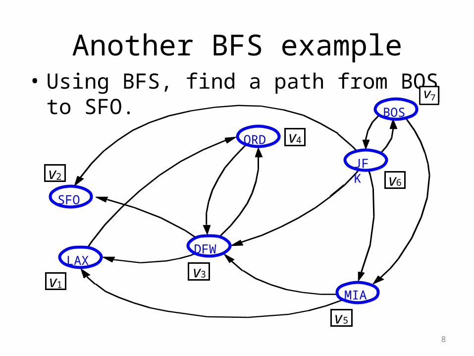
Another BFS example• Using BFS, find a path from BOS to SFO.

JFK

BOS

MIA

ORD

LAXDFW

SFO

v2

v1v3

v4

v5

v6

v7

8

DFS, BFS runtime• What is the expected runtime of DFS, in terms of the

number of vertices V and the number of edges E ?

• What is the expected runtime of BFS, in terms of the number of vertices V and the number of edges E ?

• Answer: O(|V| + |E|)– each algorithm must potentially visit every node and/or

examine every edge once.– why not O(|V| * |E|) ?

• What is the space complexity of each algorithm?9

Implementing graphs

10

Implementing a graph• If we wanted to program an actual data structure to represent a graph, what

information would we need to store?– for each vertex?– for each edge?

• What kinds of questions would we want to be able to answer quickly:– about a vertex?– about its edges / neighbors?– about paths?– about what edges exist in the graph?

• We'll explore three common graph implementation strategies:– edge list, adjacency list, adjacency matrix

12

3

4

56

7

11

Edge list• edge list: an unordered list of all edges in the graph

• advantages– easy to loop/iterate over all edges

• disadvantages– hard to tell if an edge

exists from A to B– hard to tell how many edges

a vertex touches (its degree)

1

2

1

5

1

6

2

7

2

3

3

4

5

7

5

6

5

4

7

4

12

3

4

56

7

12

Adjacency matrix• adjacency matrix: an n × n matrix where:

– the nondiagonal entry aij is the number of edges joining vertex i and vertex j (or the weight of the edge joining vertex i and vertex j)

– the diagonal entry aii corresponds to the number of loops (self-connecting edges) at vertex i

13

Pros/cons of Adj. matrix

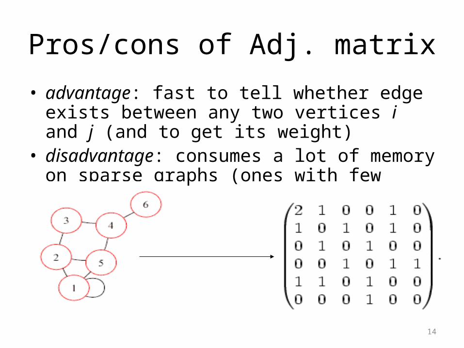
• advantage: fast to tell whether edge exists between any two vertices i and j (and to get its weight)

• disadvantage: consumes a lot of memory on sparse graphs (ones with few edges)

14

Adjacency matrix example

• The graph at right has the following adjacency matrix:– How do we figure out the degree of a given vertex?– How do we find out whether an edge exists from A to B?– How could we look for loops in the graph?

12

3

4

56

7

0100110

1234567

1010001

0101000

0010101

1001011

1000100

0101100

1 2 3 4 5 6 7

15

Adjacency lists

• adjacency list: stores edges as individual linked lists of references to each vertex's neighbors– generally, no information needs to be stored in the edges,

only in nodes, these arrays can simply be pointers to other nodes and thus represent edges with little memory requirement

16

Pros/cons of adjacency list• advantage: new nodes can be added to the graph easily, and they can be

connected with existing nodes simply by adding elements to the appropriate arrays; "who are my neighbors" easily answered

• disadvantage: determining whether an edge exists between two nodes requires O(n) time, where n is the average number of incident edges per node

17

Adjacency list example

• The graph at right has the following adjacency list:– How do we figure out the degree of a given vertex?– How do we find out whether an edge exists from A to B?– How could we look for loops in the graph?

12

3

4

56

71234567

2 5 63 1 72 43 7 56 1 7 41 54 5 2

18

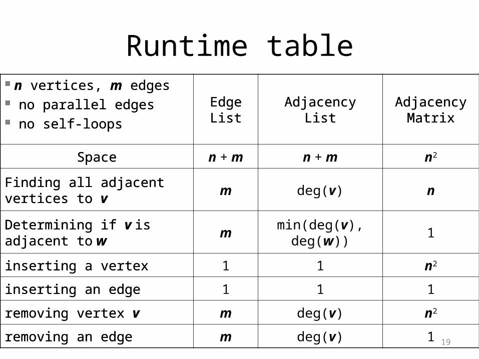
Runtime table n vertices, m edges no parallel edges no self-loops

EdgeList

AdjacencyList

Adjacency Matrix

Space

Finding all adjacent vertices to v

Determining if v is adjacent to w

inserting a vertex

inserting an edge

removing vertex v

removing an edge

n vertices, m edges no parallel edges no self-loops

EdgeList

AdjacencyList

Adjacency Matrix

Space n + m n + m n2

Finding all adjacent vertices to v

m deg(v) n

Determining if v is adjacent to w

mmin(deg(v),

deg(w))1

inserting a vertex 1 1 n2

inserting an edge 1 1 1

removing vertex v m deg(v) n2

removing an edge m deg(v) 1 19