CSCI 2720 Data Structures

Department of Computer ScienceUniversity of Georgia

Athens, GA 30602

Instructor: Liming Caiwww.cs.uga.edu/∼cai

0

A Tentative Schedule

Chapter 1. Introduction (1 week)Chapter 2. Algorithm analysis (0.5 weeks)∗

Chapter 3. Lists (1 week)Chapter 4. Trees (1 week)Chapter 5. Arrays and strings (1 week)Chapter 6. Implementation of Sets (1 week)Chapter 7. Dynamic dictionaries (2 weeks)Chapter 8. Sets of digital data (2 weeks)Chapter 9. Sets with special operations (1 week)Chapter 10. Memory management (1 week)Chapter 11. Sorting (2 weeks)

1

Chapter 1 Introduction

What is a data structure?

a double role: logic structure and physical representation.

example 1: a list L has two-fold meanings:(1) L = (a1, . . . , an), a set whose elements forming a linear relation;(2) how L is physically stored.

example 2: a tree T has two fold meanings:(1) a tree is a set whose elements forming a tree relation;(2) how T is stored.

2

The goals for data structure studies

Choosing a good data structure should

(1) facilitate algorithm design, programming, debugging, etc.[examples?]

(2) minimize the usage of computing resources. [examples?]

3

Von Neumann computer architecture

The concept of stored programs.

how is the following code executed?

example:......

x = y + 5;

A[x] = z*z - 80;

......

(1) compilation; (static memory allocation)

(2) loading;

(3) re-addressing (dynamic linking);

(4) run;

4

Abstract data types

An ADT consists of two portions:

(1) data type: a collection of objects;

(2) a collection of operations on the data type

example:ADT list L is an ordered set of elements,upon which operations such as Length(L) and Access(L, i) may bedefined.

** ADTs as basic building blocks for programming and interfacesbetween subprograms.

** ADTs do not provide explicit implementation details.

5

Mathematical background

(1) the growth of functions, the big-O notation

(2) logarithms and exponentials

(3) recurrence relations

example: Fibonacci sequenceF (n) = F (n− 1) + F (n− 2)F (1) = 1F (2) = 1Different algorithms:(1) recursive, recurrence for time complexity(2) recursive + memorizing results(3) iterative

(4) solve recurrences

expanding simple recurrence

6

Analysis of Insertion Sort

INSERTION-SORT(A)

1 for j <-- 2 to length[A]

2 do key <-- A[j]

3 /* Insert A[j] into sorted A[1..j-1] */

4 i=j-1

5 while i>0 and A[i] >key

6 do A[i+1] <-- A[i]

7 i=i-1

8 A[i+1] <-- key

Assume tj to be the number of times while is executed for every j.

T (n) = c1n+ c2(n− 1) + c4(n− 1) + c5n∑

j=2

tj + c6n∑

j=2

(tj − 1) +

c7n∑

j=2

(tj − 1) + c8(n− 1)

7

Then for some a, b, c,

T (n) ≤ an∑

j=2

tj + bn+ c — (1)

and for some d, ef ,

T (n) ≥ dn∑

j=2

tj + en+ f — (2)

The best case is when the list is already sorted: tj = 1The worst case is when the list is reversally sorted: tj = j

So we have to use tj = j. We haveT (n) ≤ xn2 + yn+ z for some x, y, z, where x > 0 — (3)

denoted as T (n) = O(n2)T (n) ≥ un2 + vn+ w for some u, v, w, where u > 0 — (4)

denoted as T (n) = Ω(n2)

Concluded: T (n) = θ(n2).

8

Complexity issues

size of the input: n, the number of bits used to encode the input.

For some problems, we may use different definitions of the inputsize.

running time of an algorithm: t(n), the number of primitiveoperations executed, defined as a function in the input size n.

worst-case running time: the upper bound on running time forany input.

average-case running time: the running time ”on average” orrunning time on a randomly chosen input assuming all inputs of agiven size (n) are equally likely.

order of growth: e.g., an2 + bn+ c, the growth rate depends onan2 as n grows if a > 0.

9

Pseudocode conventions

(1) indentation for block structure;

(2) ← for assignment, multiple assignments: x← y ← z is same asy ← z and then x← y;

(3) only local variables are allowed;

(4) A[i..j] is the subarrray of elements A[i],...A[j];

(5) call-by-value in parameter passing.

10

Analyzing algorithms

(1) random-access machine (RAM)

(2) primitive operations: add, substract, floor, ceiling, multiply,jump, memory movement, etc. difference: a constant multiplicativefactor.

(3) speed between different machines: a constant multiplicativefactor.

(4) Turing machine model, the O(log n) factor.

11

There are some divide-and-conquer approaches for Sorting Problem.

e.g., ”splitting a list into two of equal size” leads to Merge-Sortalgorithm

MERGE-SORT(A, p, r)

1 if p<r

2 then q <--(p+r)/2

3 MERGE-SORT(A, p, q)

4 MERGE-SORT(A, q+1, r)

5 MERGE(A, p, q, r)

12

Analysis of Merge-Sort

n = r − p+ 1, assume that n is a power of 2.

(1) time for divide: c1 for split the list into two sublists;

(2) time for conquer: 2T (n/2) for recursively solve subproblems

(3) time for combine: c2n for merging two length n/2 sortedsublists;

Recurrence:

T (n) = 2T (n/2) + c2n+ c1 when n > 1

T (n) = 0 when n = 1

How to solve the recurrence?

13

T (n) = 2T (n/2) + c2n+ c1

2T (n/2) = 22T (n/22) + 2c2n/2 + 2c1

22t(N/22) = 23T (n/23) + 22c2/22 + 22c1

· · ·

2kT (n/2k) = 2k+1T (n/2k+1) + 2kc2n/2k + 2kc1

Let n/2k+1 = 1 then k + 1 = log2 n

Then T (n) = 2k+1T (1) + (k + 1)c2n+ c1k∑

i=0

2i

T (n) = 0 + c2n log2 n+ c1(2k+1 − 1) = c2n log2 n+ c1(n− 1)

14

How fast does T (n) grow?

When n is big enough, there is a constant a > 0 such that

T (n) ≤ an log2 n.

T (n) cannot grow faster than an log2 n for some constant a > 0.

Apparently, there is a constant b > 0 such that

T (n) ≥ bn log2 n

T (n) grows faster than bn log2 n when n is large enough.

15

Growth of functions

Asymptotic notation

O(g(n)) = f(n) : ∃c > 0, n0 > 0 such that0 ≤ f(n) ≤ cg(n), for all n ≥ n0

Ω(g(n)) = f(n) : ∃c > 0, n0 > 0 such that0 ≤ cg(n) ≤ f(n), for all n ≥ n0

Θ(g(n)) = f(n) : ∃c1 > 0, c2 > 0, n0 > 0 such thatc1g(n) ≤ f(n) ≤ c2g(n), for all n ≥ n0

16

other notations and functions

floors and ceilingsmodular arthmeticpolynomialsexponentialslogarithmsStirling’s approximation n! =

√2πn(n/e)n(1 + Θ(1/n))

Fibonacci numbers:

17

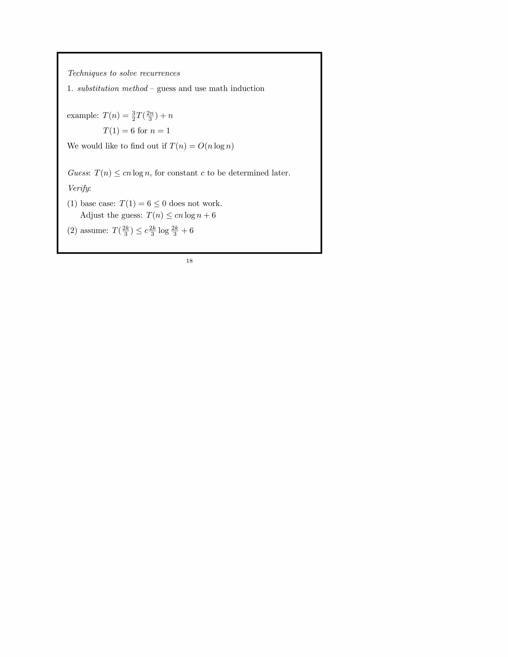
Techniques to solve recurrences

1. substitution method – guess and use math induction

example: T (n) = 32T ( 2n

3 ) + n

T (1) = 6 for n = 1

We would like to find out if T (n) = O(n log n)

Guess: T (n) ≤ cn log n, for constant c to be determined later.

Verify:

(1) base case: T (1) = 6 ≤ 0 does not work.Adjust the guess: T (n) ≤ cn log n+ 6

(2) assume: T ( 2k3 ) ≤ c 2k

3 log 2k3 + 6

18

(3) induction:

T (k) = 32T ( 2k

3 ) + k

≤ 32 (c 2k

3 log 2k3 + 6) + k

= ck log 2k3 + 9 + k

= ck(log k − log 3/2) + 9 + k

= ck log k + k − ck(log 3/2) + 3 + 6= ck log k + k[1− c(log 3/2) + 3/k] + 6≤ ck log k + 6

when 1− c(log 3/2) + 3/k < 0 which can hold by choosing c = 4and k > 3.

So we have shown that

T (n) ≤ 4n log n+ 6 when n > n0 = 3. That is

T (n) = O(n log n)

19

Can you use the substitution method to show T (n) = Ω(n log n)?

which part of the proof for T (n) = O(n log n) needs to be changed?

20

2. changing variables

example: T (n) = 2T (√n) + log2 n

define m = log2 n, i.e., n = 2m

then T (2m) = 2T (2m/2) +m

rename the function: S(m) = T (2m)

S(m) = 2S(m/2) +m

solve it, we have S(m) = O(m logm)

so T (n) = T (2m) = O(m logm) = O(log n log log n).

21

3. recursive tree method

also based on unfolding the recurrence to make a recursive-tree.

(1) T (n) is a tree with non-recursive terms as the root andrecursive terms as its children.

(2) for each child, replace it with then non-recursive terms andproducing children that are then recursive terms

(3) repeat (2), expand the tree until all children are the base case.

22

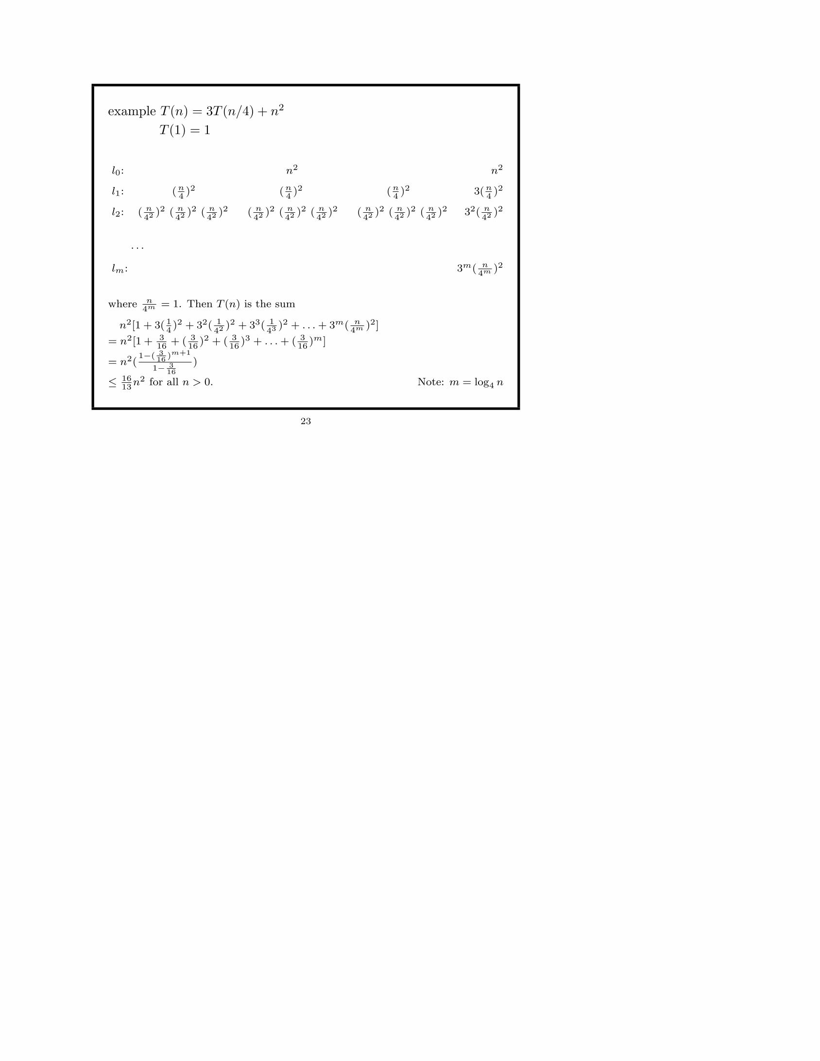
example T (n) = 3T (n/4) + n2

T (1) = 1

l0: n2 n2

l1: (n4)2 (n

4)2 (n

4)2 3(n

4)2

l2: ( n42 )2 ( n

42 )2 ( n42 )2 ( n

42 )2 ( n42 )2 ( n

42 )2 ( n42 )2 ( n

42 )2 ( n42 )2 32( n

42 )2

· · ·

lm: 3m( n4m )2

where n4m = 1. Then T (n) is the sum

n2[1 + 3( 14)2 + 32( 1

42 )2 + 33( 143 )2 + . . . + 3m( n

4m )2]

= n2[1 + 316

+ ( 316

)2 + ( 316

)3 + . . . + ( 316

)m]

= n2(1−( 3

16 )m+1

1− 316

)

≤ 1613

n2 for all n > 0. Note: m = log4 n

23

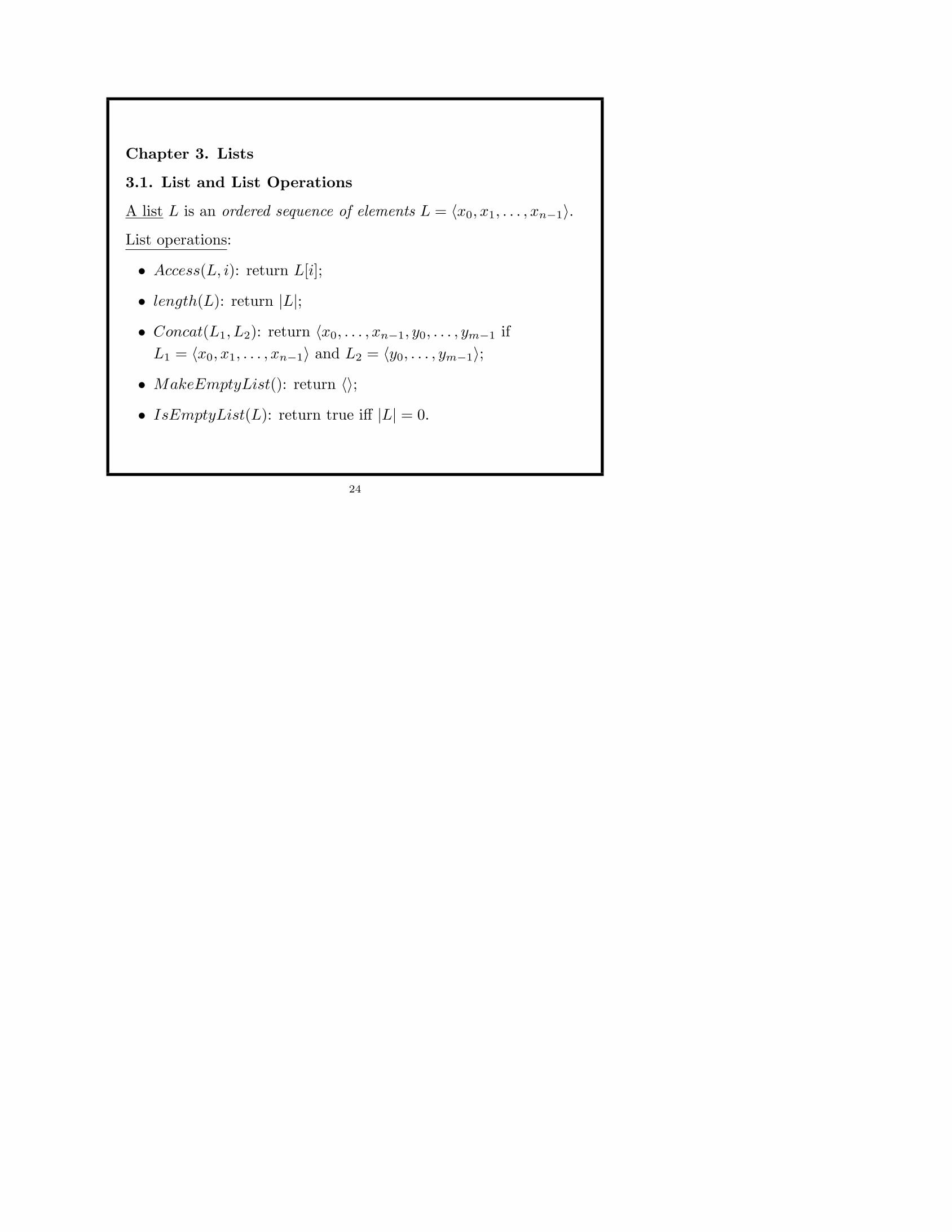
Chapter 3. Lists

3.1. List and List Operations

A list L is an ordered sequence of elements L = 〈x0, x1, . . . , xn−1〉.

List operations:

• Access(L, i): return L[i];

• length(L): return |L|;

• Concat(L1, L2): return 〈x0, . . . , xn−1, y0, . . . , ym−1 ifL1 = 〈x0, x1, . . . , xn−1〉 and L2 = 〈y0, . . . , ym−1〉;

• MakeEmptyList(): return 〈〉;

• IsEmptyList(L): return true iff |L| = 0.

24

Special cases of lists:

stack: is a list.

• Top(L): return the last element of L;

• Pop(L): remove and return the last element of L;

• Push(x, L): Concat(L, 〈x〉);

• MakeEmptyStack();

• IsEmptyStack(L);

25

Special cases of lists:

queue: is a list.

• Enqueue(x, L): Concat(L, 〈x〉);

• Dequeue(L); remove and return the first element of L;

• Front(L): return the first element of L;

• MakeEmptyQueue(); return 〈〉;

• IsEmptyQueue(L);

26

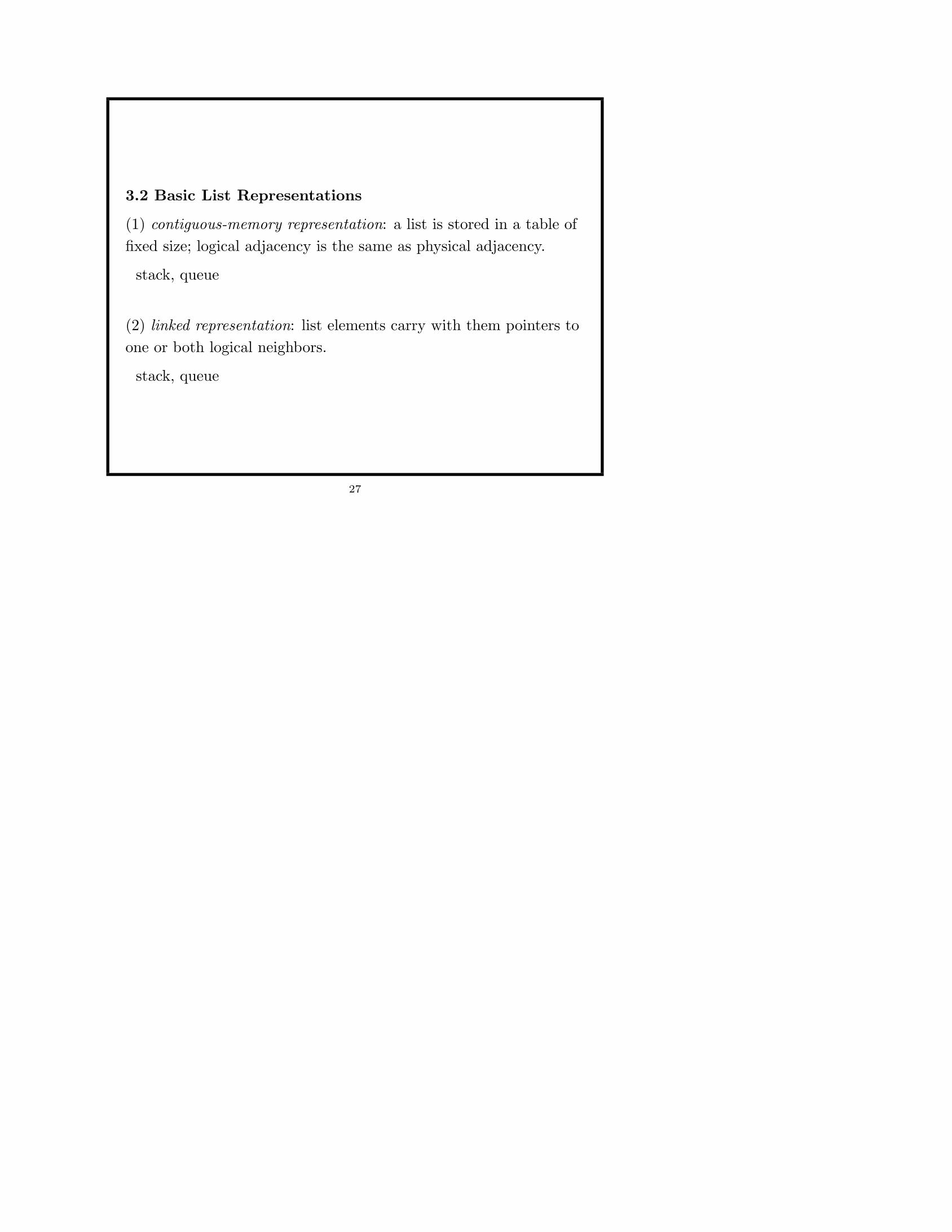
3.2 Basic List Representations

(1) contiguous-memory representation: a list is stored in a table offixed size; logical adjacency is the same as physical adjacency.

stack, queue

(2) linked representation: list elements carry with them pointers toone or both logical neighbors.

stack, queue

27

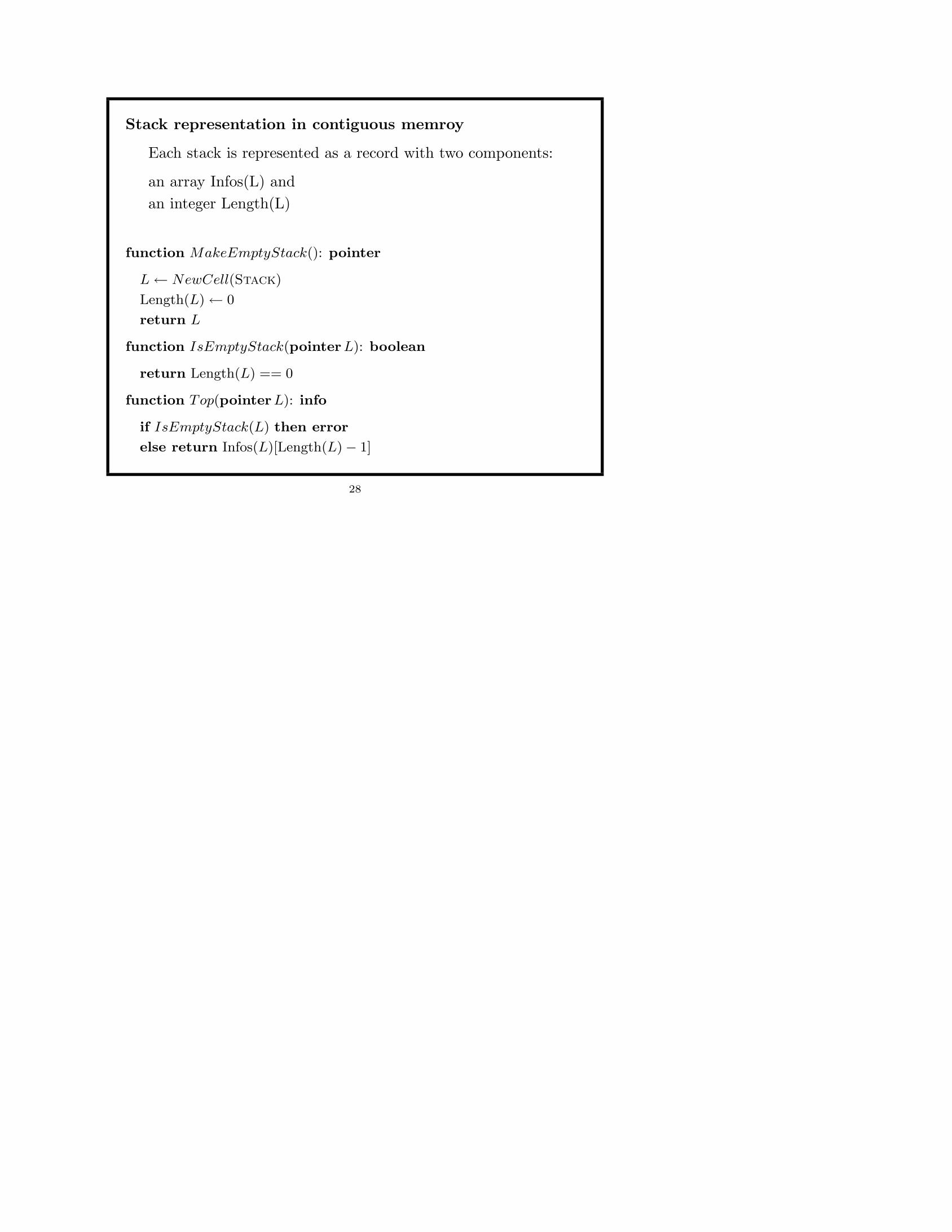
Stack representation in contiguous memroy

Each stack is represented as a record with two components:

an array Infos(L) andan integer Length(L)

function MakeEmptyStack(): pointer

L← NewCell(Stack)

Length(L)← 0

return L

function IsEmptyStack(pointerL): boolean

return Length(L) == 0

function Top(pointerL): info

if IsEmptyStack(L) then error

else return Infos(L)[Length(L)− 1]

28

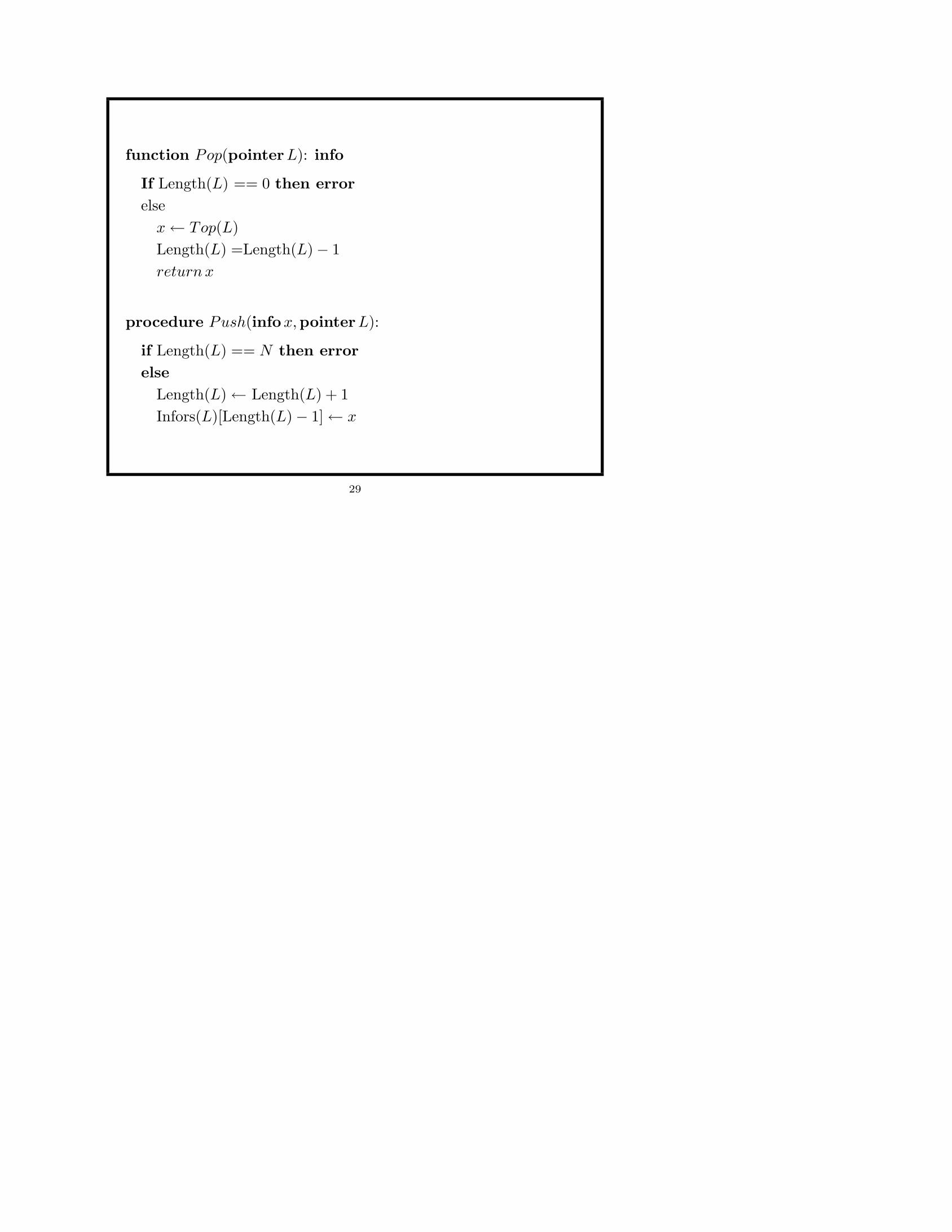
function Pop(pointerL): info

If Length(L) == 0 then errorelsex← Top(L)Length(L) =Length(L)− 1return x

procedure Push(infox,pointerL):

if Length(L) == N then errorelse

Length(L)← Length(L) + 1Infors(L)[Length(L)− 1]← x

29

Queue representation in contiguous memroy

Each queue is represented as a record with three components:

an array Infos(L)an integer Length(L) andan integer Front(L)

function MakeEmptyQueue(): pointer

L← NewCell(Queue)

Length(L)← 0

Front(L)← 0

return L

function IsEmptyQueue(pointerL): boolean

return Length(L) == 0

30

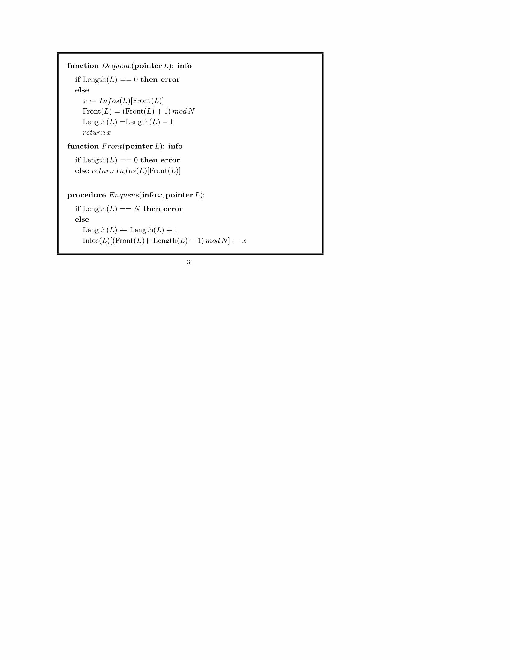
function Dequeue(pointerL): info

if Length(L) == 0 then error

else

x← Infos(L)[Front(L)]

Front(L) = (Front(L) + 1) mod N

Length(L) =Length(L)− 1

return x

function Front(pointerL): info

if Length(L) == 0 then error

else return Infos(L)[Front(L)]

procedure Enqueue(infox,pointerL):

if Length(L) == N then error

else

Length(L)← Length(L) + 1

Infos(L)[(Front(L)+ Length(L)− 1) mod N ]← x

31

Stack representation in linked memory

Each stack is represented as a linked list of nodes,each of which consists of two components:

an data Info andan pointer Next

function MakeEmptyStack() : pointer

return Λ

function IsEmptyStack(pointerL): boolean

return L == Λ

function Top(pointerL): info

if L == Λ then error

else return Info(L)

32

function Pop(pointerL): info

if L == Λ then errorelsex← Top(L)L← Next(L)return x

procedure Push(infox,pointerL):

P ← NewCell(Node)Info(P )← x

Next(P )← L

L← P

33

Queue representations in linked memory

Each queue is represented as a record of two fields:

Front and Back, pointing to linked list nodes

function MakeEmptyQueue(): pointer

L← NewCell(Queue)

Front(L) ← Λ

Back(L) ← Λ

return L

function IsEmptyQueue(pointerL): boolean

return Front(L) == Λ

function Front(pointerL): info

if IsEmptyQueue(L) then error

else return Info(Front(L))

34

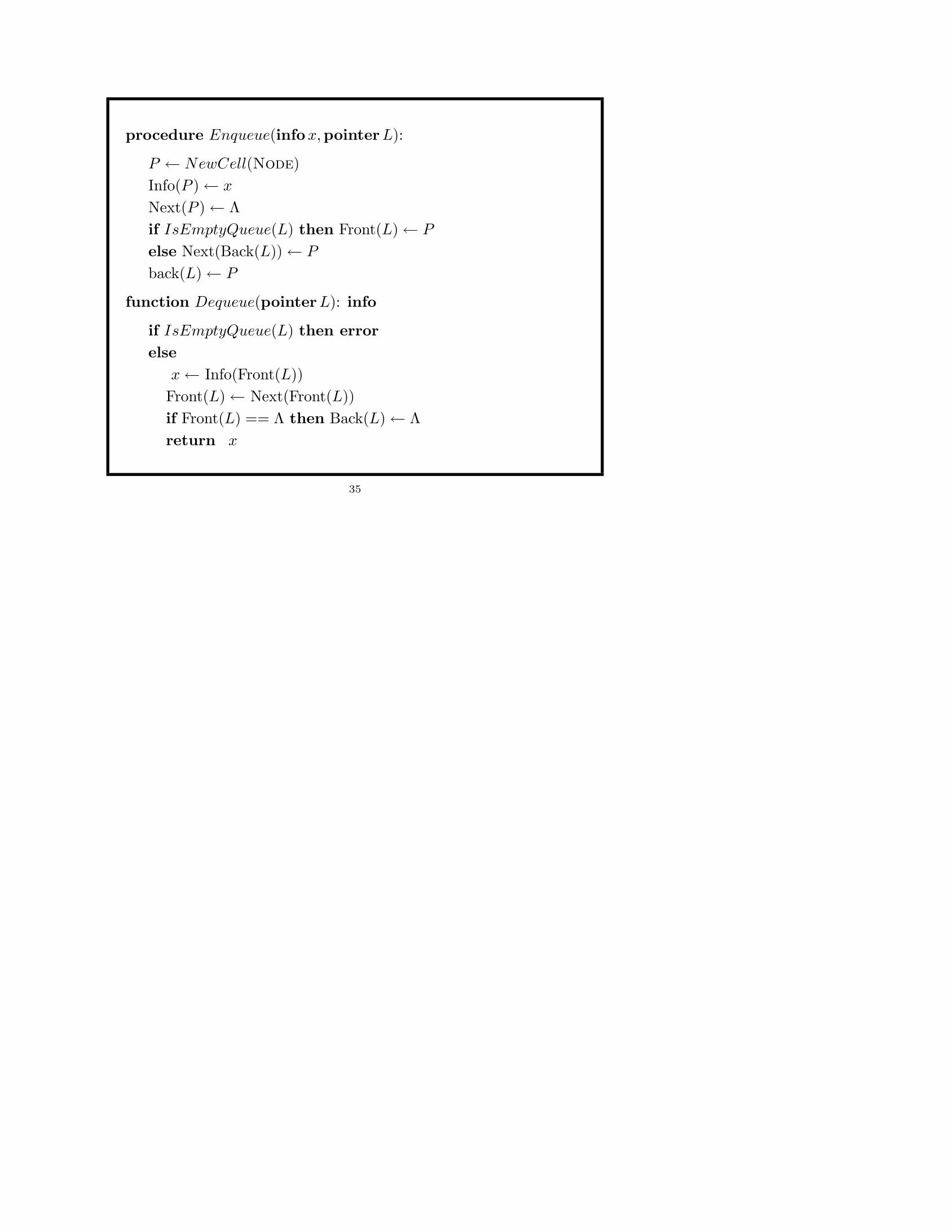
procedure Enqueue(infox,pointerL):

P ← NewCell(Node)Info(P )← x

Next(P )← Λif IsEmptyQueue(L) then Front(L)← P

else Next(Back(L))← P

back(L)← P

function Dequeue(pointerL): info

if IsEmptyQueue(L) then errorelse

x← Info(Front(L))Front(L)← Next(Front(L))if Front(L) == Λ then Back(L)← Λreturn x

35

3.3 Stacks and Recursion

Example: Merge Sort

procedure MergeSort(pointerT, integer a, b):

if a < b

then middle← b(a+ b)/2cMergeSort(T, a,middle)mergeSort(T,middle+ 1, b)Combine(T, a,middle, b)

procedure Combine(pointerL, integerhead,mid, tail)

. . .

36

procedure MergeSort(pointerT, integer a, b):On entry T, a, b and the return address are on the stack

mergesort:leave space on the stack for local variable midif a ≥ b then goto exit

mid← b(a+ b)/2cPush(return1, S);Push(T, S);Push(a, S);Push(mid, S)goto mergesort

return1:Push(return2, S);Push(T, S);Push(mid+ 1, S);Push(b, S)goto mergesort

return2:merge two sorted sublists into one

exit: discard local variables, Pop and goto return address

37

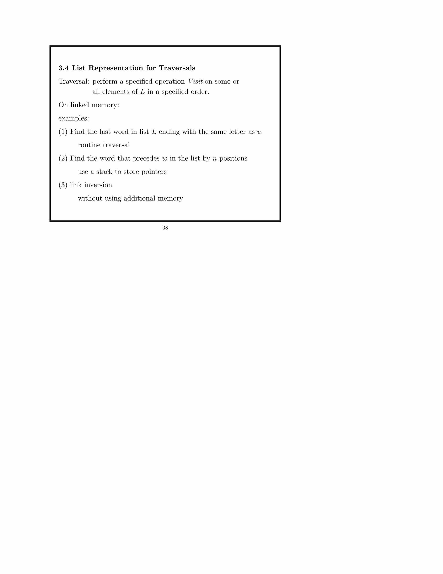
3.4 List Representation for Traversals

Traversal: perform a specified operation Visit on some orall elements of L in a specified order.

On linked memory:

examples:

(1) Find the last word in list L ending with the same letter as w

routine traversal

(2) Find the word that precedes w in the list by n positions

use a stack to store pointers

(3) link inversion

without using additional memory

38

3.5 Doubly Linked Lists

operations:

deletion example

insertion example

”pointer compression”: exclusive-OR coded doubly linked list

39

Chapter 4. Trees

4.1 Basic definitions

4.2 Special kinds of trees

4.3 Tree operations and traversals

4.4 Tree implementations

4.5 Implementing tree traversals and scans

40

4.1 Basic Definitions

nodes, edges, root

Tree are defined recursively

1. a single node, with no edges, is a tree. The root of the tree is itsunique node.

2. Let T1, . . . , Tk be trees with no nodes in common, and r1, . . . , rk

be the roots of these trees, respectively. Let r be a new node. ThenT consisting of the modes and edges of T1, . . . , Tk, the new node r,and new edges 〈r, r1〉, . . . , 〈r, rk〉, is a tree. The root of the tree T isr. T1, . . . , Tk are called subtrees of T .

41

Other terms: parent, children, siblings, descendant, ancestor, path,leaf

height of a node: the length of the longest path from the node to aleaf.

depth of a node: the length of path from the root to the node.

42

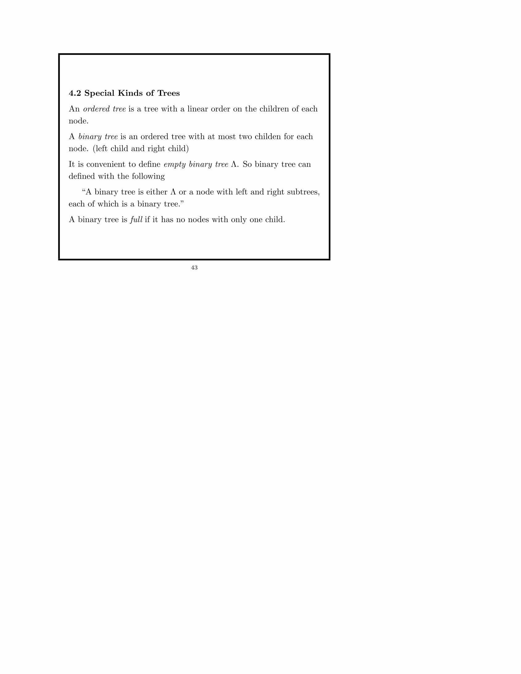
4.2 Special Kinds of Trees

An ordered tree is a tree with a linear order on the children of eachnode.

A binary tree is an ordered tree with at most two childen for eachnode. (left child and right child)

It is convenient to define empty binary tree Λ. So binary tree candefined with the following

“A binary tree is either Λ or a node with left and right subtrees,each of which is a binary tree.”

A binary tree is full if it has no nodes with only one child.

43

A perfect binary tree is a full binary tree in which all leaves havethe same depth.

Theorem: a perfect binary tree of height h has 2h+1 − 1 nodes,with 2h leaves and 2h − 1 nonleaves.

A complete binary tree:

(1) a complete binary tree of height 0 is a single node;

(2) a complete binary tree of height 1 is a tree of height 1 with

either two children or a left child only;

(3) For h ≥ 2, a complete binary tree of height h is a root with

two subtree satisfying one of these two conditions:

(a) the left subtree is a perfect binary tree of height h− 1 and the

right subtree is a complete binary tree of height h− 1,

(b) the left subtree is a complete binary tree of height h− 1 and

the right subtree is a perfect binary tree of height h− 2.

44

Any ordered tree can be converted to a binary tree. How?

45

4.3 Tree Operations and Traversals

Given node v, the following operations:

Parent(v): return the parent of vChildren(v); return the set of children of vF irstChild(v): return the first child of vRightSibling(v): return the right sibling of vLeftSibling(v):LeftChild(v), RightChild(v)IsLeaf(v), Depth(v), Height(v).

We first discuss some applications of these operations.

46

Arithmetic expression evaluations

Infix expressions such as 20× 2 + 3 can be described by full binarytrees.

function Evaluate(pointerP ) : integerif IsLeaf(P ) then return Label(P )else

xL ← Evaluate(LeftChild(P ))xR ← Evaluate(RightChild(P ))op← Label(P )return ApplyOP (op, xL, xR)

47

Traversals on trees: postorder, inorder, and preorder

procedure Postorder(pointerP ) :for each child Q of P , in order do

Postorder(Q)V isit(P )

procedure Pretorder(pointerP ) :V isit(P )for each child Q of P , in order do

Pretorder(Q)

procedure Inorder(pointerP ) :if P = Λ then returnelse

Inorder(LeftChild(P ))V isit(P )Inorder(RightChild(P ))

48

4.4 Tree Implementations

representation of binary trees

the standard representation: LC, RC,

representation of ordered trees

binary trees, ternary trees, k-ary trees

binary tree representation of ordered trees:

FirstChild and RightSilbing

representation of complete binary

without pointer in contiguous memory

49

4.5 Implementing Tree Traversals and Scans

stack-based traversals

recursive traversal, for example:

procedure InorderTraversal(pointerP ):

if P 6= Λ then

InorderTraversal(LC(P ))

visit(P )

InorderTraversal(RC(P ))

50

Non-recursive traversal how to refine the following algorithm?

keep push to stack of current node, go to its left child

until its left child is empty

pop the stack and visit the node just popped

let the current node be the right child

repeat whole thing

51

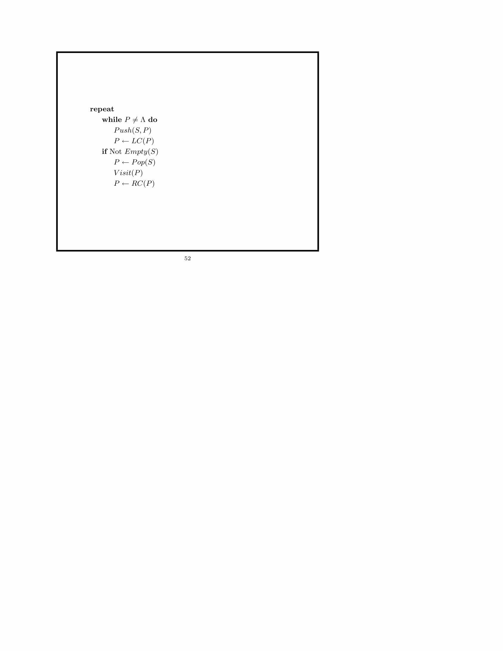
repeat

while P 6= Λ do

Push(S, P )

P ← LC(P )

if Not Empty(S)

P ← Pop(S)

V isit(P )

P ← RC(P )

52

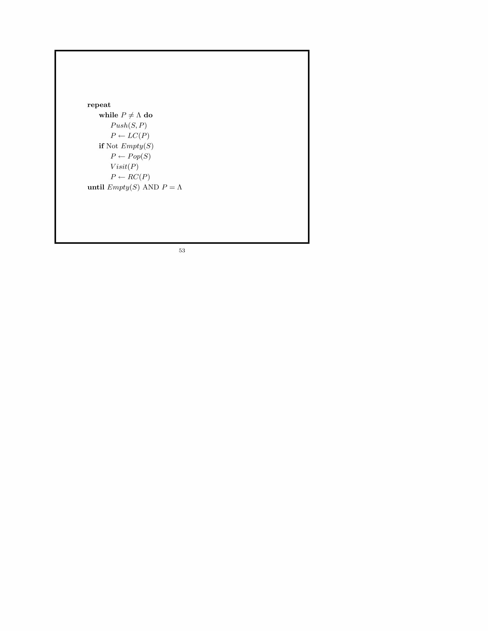
repeat

while P 6= Λ do

Push(S, P )

P ← LC(P )

if Not Empty(S)

P ← Pop(S)

V isit(P )

P ← RC(P )

until Empty(S) AND P = Λ

53

Now how to do pre-order and post-order traversals with a stack?

which parts to modify?

repeat

while P 6= Λ do

Push(S, P )

P ← LC(P )

if Not Empty(S)

P ← Pop(S)

V isit(P )

P ← RC(P )

until Empty(S) AND P = Λ

54

Computing the height of a binary tree

the height of the root is the max heightbetween its left and right child

recursive, which mode of traversal is suitable?

idea:

how about using non-recursive traversal?

idea:

55

The height of the stack needed is the height of the binarytree

Where to compute the height?

repeat

while P 6= Λ do

Push(S, P )

P ← LC(P )

if Not Empty(S)

P ← Pop(S)

V isit(P )

P ← RC(P )

until Empty(S) AND P = Λ

56

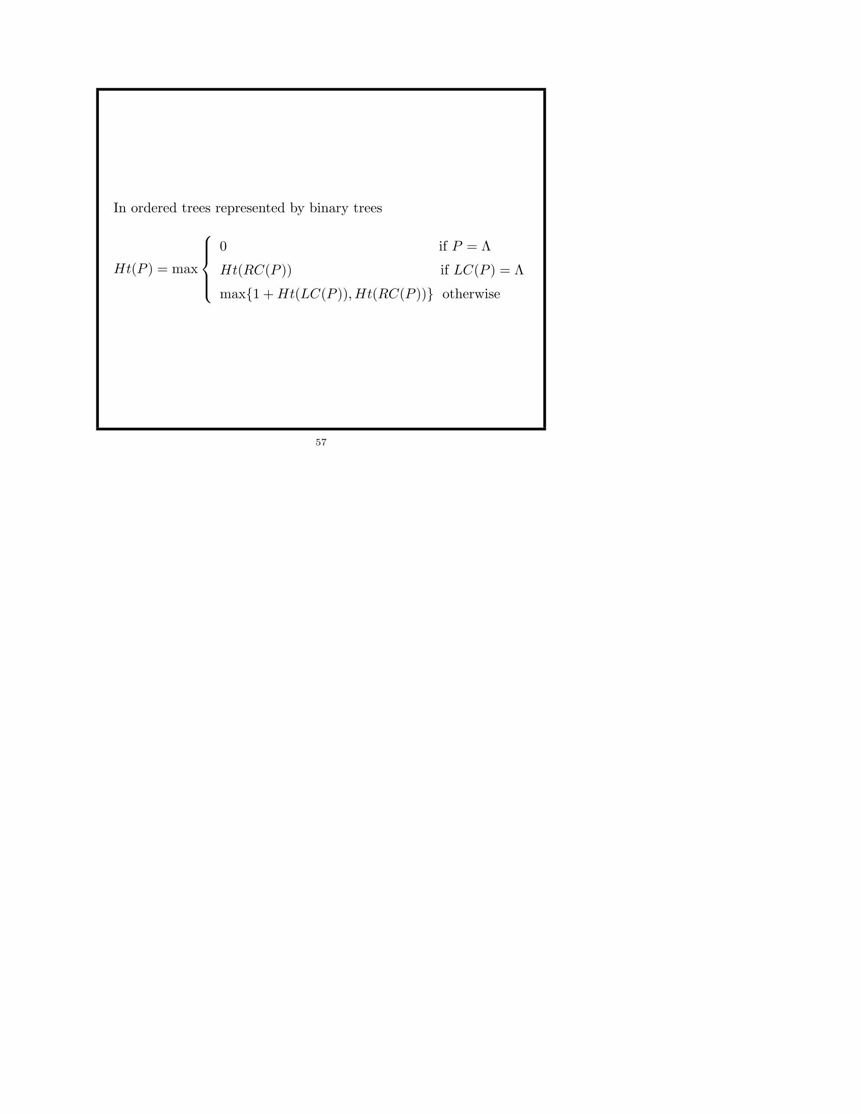
In ordered trees represented by binary trees

Ht(P ) = max

0 if P = Λ

Ht(RC(P )) if LC(P ) = Λ

max1 +Ht(LC(P )), Ht(RC(P )) otherwise

57

link-inversion traversal

when the structure of the tree can be altered during the traversal

In each of the following groups, statements are executed simultaneously:

descend to left: P ← Q

Q← LC(Q)

LC(Q)← P

descend to right: P ← Q

Q← RC(Q)

RC(Q)← P

ascend from left: Q← P

P ← LC(P )

LC(P )← Q

ascend from right: Q← P

P ← RC(P )

RC(P )← Q

58

procedure LinkInversionTraverse(pointerQ):

P ← Λ

repeat forever

while Q 6= Λ do

Tag(Q)← 0

descend to left

while P 6= Λ and Tag(P ) = 1 do

ascend from right

if P = Λ then return

else

ascend from left

visit(Q)

Tag(Q) = 1

descend to right

59

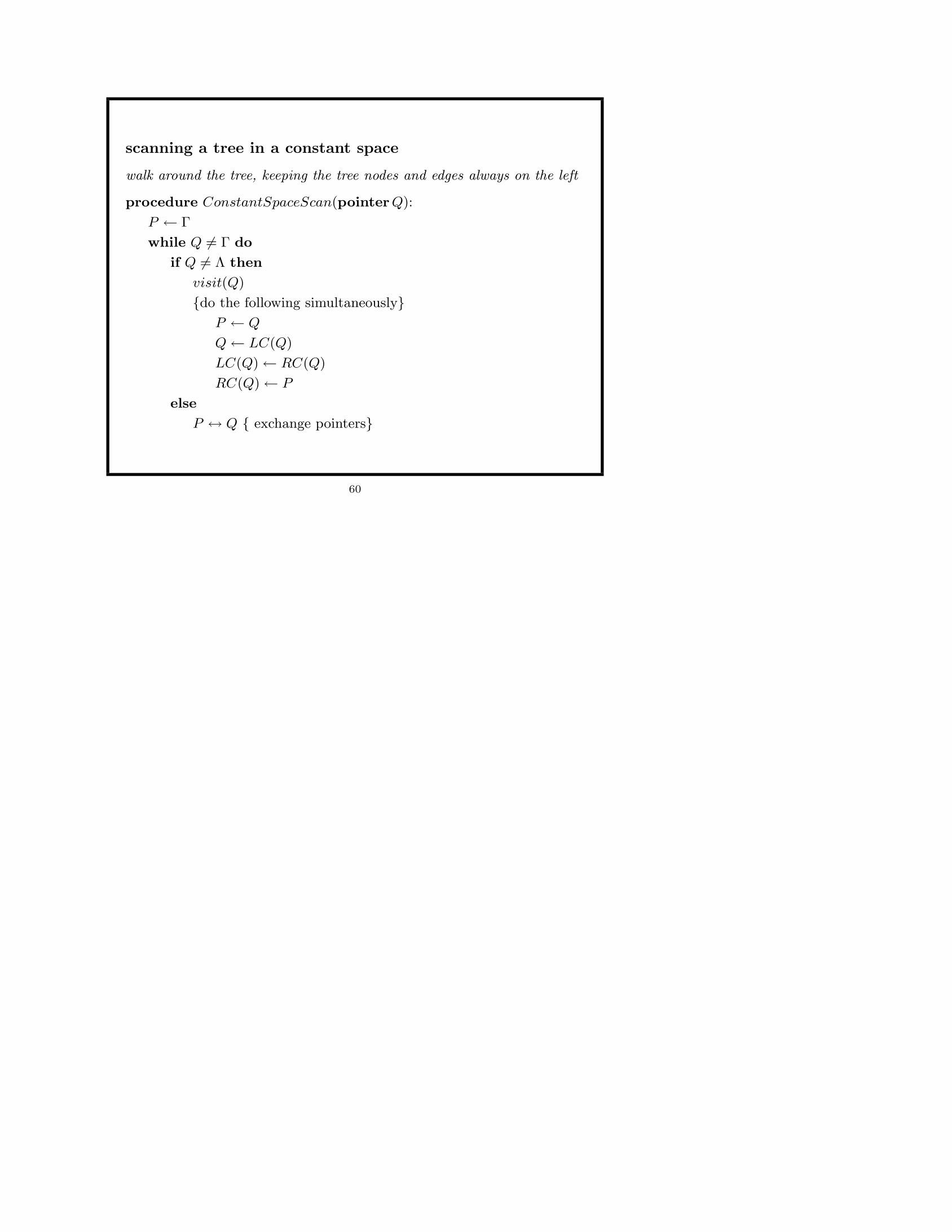
scanning a tree in a constant space

walk around the tree, keeping the tree nodes and edges always on the left

procedure ConstantSpaceScan(pointerQ):

P ← Γ

while Q 6= Γ do

if Q 6= Λ then

visit(Q)

do the following simultaneouslyP ← Q

Q← LC(Q)

LC(Q)← RC(Q)

RC(Q)← P

else

P ↔ Q exchange pointers

60

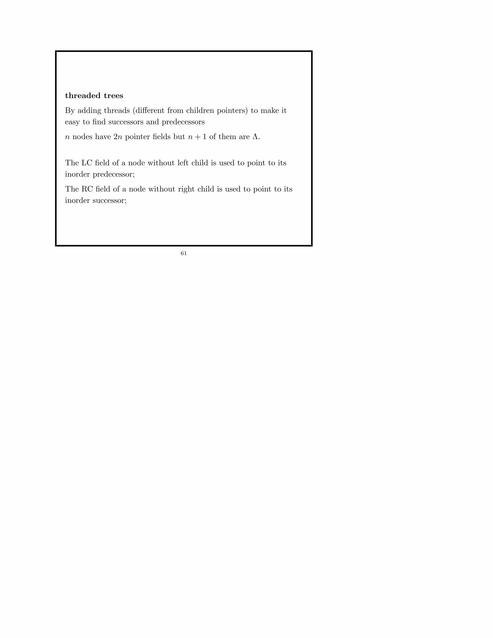
threaded trees

By adding threads (different from children pointers) to make iteasy to find successors and predecessors

n nodes have 2n pointer fields but n+ 1 of them are Λ.

The LC field of a node without left child is used to point to itsinorder predecessor;

The RC field of a node without right child is used to point to itsinorder successor;

61

function InorderSuccessor(pointerN) : pointer

P ← RC(N)

if P = Λ then return Λ

else if P is not a thread then

while LC(P ) is not a thread or Λ do

P ← LC(P )

return P

How much time is needed to find the successor?

62

function PreorderSuccessor(pointerN) : pointer

if LC(N) is not a thread and is not Λ then return LC(N)

else

P ← N

while RC(P ) is a thread do

P ← RC(P )

if RC(N) = Λ then return Λ

else return RC(P )

How much time is needed to find the successor?

63