CSCI 256

Data Structures and Algorithm Analysis

Lecture 3

Some slides by Kevin Wayne copyright 2005, Pearson Addison Wesley all rights reserved, and some by Iker Gondra

Computational Tractability

• A major focus of algorithm design is to find efficient algorithms for computational problems. What does it mean for an algorithm to be efficient?

As soon as an Analytic Engine exists, it will necessarily guide the future course of the science. Whenever any result is sought by its aid, the question will arise - By what course of calculation can these results be arrived at by the machine in the shortest time? - Charles Babbage

Charles Babbage (1864) Analytic Engine (schematic)

Some Initial Attempts at Defining Efficiency

• Proposed Definition of Efficiency (1): An algorithm is efficient if, when implemented, it runs quickly on real input instances– Where does it run? Even bad algorithms can run quickly when

applied to small test cases on extremely fast processors – How is it implemented? Even good algorithms can run slowly

when they are coded sloppily– What is a “real” input instance? Some instances can be much

harder than others– How well, or badly, does the running time scale as problem sizes

grow to unexpected levels?– We need a concrete definition that is platform-independent,

instance-independent, and of predictive value with respect to increasing input sizes

Worst-Case Analysis

• Worst case running time: Obtain bound on largest possible running time of algorithm on input of a given size N– Draconian view, but hard to find effective alternative– Generally captures efficiency in practice

• Average case running time: Obtain bound on some averaged running time of algorithm on some random input as a function of input size N– Hard (or impossible) to accurately model real instances by

random distributions– Algorithm tuned for a certain distribution may perform poorly on

other inputs

Brute-Force Search

• Ok, but what is a reasonable analytical benchmark that can tell us whether a running time bound is impressive or weak?– For many non-trivial problems, there is a natural brute force

search algorithm that checks every possible solution (i.e., try all possibilities, see if any one works, n! for Stable Matching (n = number of pairs of men and women)

– Note that this is an intellectual cop-out; it provides us with absolutely no insight into the problem structure

– Thus, a first simple guide is by comparison with brute-force search

• Proposed Definition of Efficiency (2): An algorithm is efficient if it achieves qualitatively better worst-case performance than brute-force search– Still vague, what is “qualitatively better performance”?

Polynomial Time as a Definition of Efficiency

• Desirable scaling property: Algorithms with polynomial run time have the property that: increasing the problem size by a constant factor increases the run time by at most a constant factor

• An algorithm is polynomial-time if the above scaling property holds

There exists constants c > 0 and d > 0 such that on every input of size N, its running time is bounded by cNd steps.

Polynomial Time as a Definition of Efficiency

• In the above if we increase input from N to 2N then the running time is c(2N)d = c2dNd, which is a slow down of a factor of 2d which is a constant since d is a constant

• Note: for stable matching problem N the size of the input is really 2n2, where n = number of men

– Why? – well there are n men and n women and each has a preference list of size n so the size of the input N = 2n x n = 2n2

Polynomial Time as a Definition of Efficiency

• Proposed Definition of Efficiency (3): An algorithm is efficient if it has a polynomial running time.

• (n100 is polynomial and n (1 + .002(logn)) is not; generally we would be happier with the second running time; BUT:

• Polynomial running time as a notion of efficiency really works in practice!– Generally, polynomial time seems to capture the algorithms which

are efficient in practice– Although 6.02 1023 N20 is technically polynomial-time, it would

be useless in practice

– In practice, the polynomial-time algorithms that people develop almost always have low constants and low exponents

– Breaking through the exponential barrier of brute force typically exposes some crucial structure of the problem

Polynomial Time as a Definition of Efficiency

• One further reason why the mathematical formalism and the empirical evidence seem to line up well in the case of polynomial-time solvability is that the gulf between the growth rates of polynomial and exponential functions is enormous

Asymptotic Order of Growth

• We could give a very concrete statement about the running time of an algorithm on inputs of size N such as: On any input of size N, the algorithm runs for at most 1.62N2 + 3.5N + 8 steps– Finding such a precise bound may be an exhausting

activity, and more detail than we wanted anyway– Extremely detailed statements about the number of

steps an algorithm executes are often meaningless. Why?

Why Ignore Constant Factors?

• Constant factors are arbitrary– Depend on the implementation– Depend on the details of the architecture being used

to do the computing

• Determining the constant factors is tedious • Determining constant factors provides little

insight– A more course grained approach allows us to uncover

similarities among different classes of algorithms

Why Emphasize Growth Rates?

• The algorithm with the lower growth rate will be faster for all but a finite number of cases (small inputs)

• Performance is most important for larger problem size

• As memory prices continue to fall, bigger problem sizes become feasible

• Improving growth rate often requires new techniques

Formalizing Growth Rates

Let T(n) = the worst case running time for an algorithm with input of size n•Upper bounds: T(n) is O(f(n)) ( say: T(n) is order f(n) or T is asymptotically upper bounded by f(n) ) if there exist constants c > 0 and n0 0 such that for all n n0 we have T(n) c · f(n)

To express that an upper bound is the best possible:•Lower bounds: T(n) is (f(n)) (say: T is asymptotically lower bounded by f(n) ) if there exist constants c > 0 and n0 0 such that for all n n0 we have T(n) c · f(n)

Formalizing Growth Rates

• Tight bounds: T(n) is (f(n)) ( say: f(n) is an asymptotically tight bound for T(n) ) if T(n) is both O(f(n)) and (f(n))

• Ex: T(n) = 32n2 + 17n + 37 show:

– T(n) is O(n2), O(n3), (n2), (n), and (n2) – T(n) is not O(n), not (n3), not (n), and not (n3)

Growth Rates ctd

– Note for n ≥ 1; c = (32 + 17 + 37) works to show O(n2)– How would we do this? Try induction!!!

– Note for n ≥ 1; c = 32 works to show (n2)

– You should be able to show the following:

– Clearly if T(n) is not O(n), it is not (n)– Similarly, if T(n) is not (n3), it is not (n3)– If T(n) is O(n), it is O(n2)– If T(n) is (n3), it is (n2)

Properties of Asymptotic Growth Rates

• Of course in the previous problem the definition of lim n → ∞ is the key!!! And what is that???

Properties of Asymptotic Growth Rates

• Transitivity (proved in class)– If f = O(g) and g = O(h) then f = O(h)– If f = (g) and g = (h) then f = (h)– If f = (g) and g = (h) then f = (h)

• Additivity (proved in class)– If f = O(h) and g = O(h) then f + g = O(h) – If f = (h) and g = (h) then f + g = (h)– If f = (h) and g = O(h) then f + g = (h)

– If fi = O(h) i = 1,…,k, then f1+ f2+ …+ fk = O(h)

Recall: Properties of Exponentials

• (ax) y = axy

• a x+y = ax ay

• a x - y = ax/ay

Recall: Properties of Logs

Recall loga m = x if and only if m = ax

Ex: Show loga ax = x and a loga x = x

• loga mn = loga m + loga n

• loga m/n = loga m - loga n

• loga mx = x loga m

• loga a = 1

• Change of base: loga m = loga b logb m so:

loga m/ loga b = logb m

Here, a, b > 1; m, n, x > 0

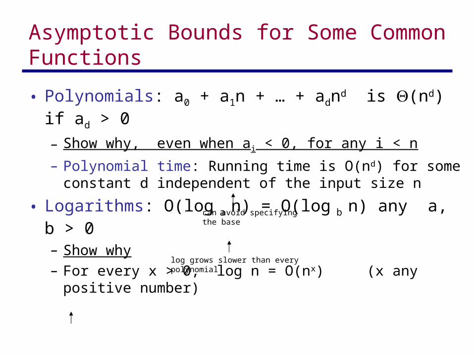
Asymptotic Bounds for Some Common Functions

• Polynomials: a0 + a1n + … + adnd is (nd) if ad > 0

– Show why, even when ai < 0, for any i < n

– Polynomial time: Running time is O(nd) for some constant d independent of the input size n

• Logarithms: O(log a n) = O(log b n) any a, b > 0– Show why– For every x > 0, log n = O(nx) (x any positive number)

can avoid specifying the base

log grows slower than every polynomial

• Exponentials: f(n) = rn

• Every exponential grows faster than every polynomial:– For every r > 1 and every d > 0, nd = O(rn)– In contrast to the situation for logs, to say a function is

exponential is somewhat sloppy: if r > s >1, it is never the case that rn = (sn)

– But we do often say that running time is exponential without specifying the base

– In general logs grow more slowly than polynomials which grow more slowly than exponentials

Exercise

• Take the following list of functions and arrange them in ascending order of growth rate. That is, if function g(n) immediately follows function f(n) in your list, then it should be the case that f(n) is O(g(n))– f1(n) = 10n

– f2(n) = n1/3

– f3(n) = nn

– f4(n) = log2n

– f5(n) = 2n/100

Common Running Times: Linear Time: O(n)

• Linear time: Running time is at most a constant factor times the size of the input– E.g., Computing the maximum: Compute maximum

of n numbers a1, …, an

max a1

for i = 2 to n { if (ai > max) max ai

}

Common Running Times:Linear Time: O(n)

– E.g., Merge: Combine two sorted lists A = a1,a2,…,an with B = b1,b2,…,bn into sorted whole

– Claim: Merging two lists of size n takes O(n) time• Pf: After each comparison, the length of output list increases by 1

i = 1, j = 1while (both lists are nonempty) { if (ai bj) append ai to output list and increment i else append bj to output list and increment j}append remainder of nonempty list to output list

Common Running Times: O(n log n) Time

• O(n log n) time: Arises in divide-and-conquer algorithms (we will see that this is an algorithm that splits its input in half, solves each recursively and combines the pieces in linear time)• Sorting: Mergesort and heapsort are sorting algorithms that

perform O(n log n) comparisons

• Frequently we find algorithms with running time O(n log n) because there are many algorithms where the most expensive step is to sort the input.

Common Running Times:Quadratic Time: O(n2)

• Quadratic time: – E.g., Closest pair of points: Given a list of n points in the plane

(x1, y1), …, (xn, yn), find the pair that is closest

– Here’s a O(n2) solution: Try all pairs of points

– Remark: (n2) seems inevitable but, as we will see, this is just an illusion

min (x1 - x2)2 + (y1 - y2)2

for i = 1 to n { for j = i+1 to n { d (xi - xj)2 + (yi - yj)2

if (d < min) min d }}

Common Running Times: Cubic Time: O(n3)

• Cubic time: E.g., Set disjointness: Given n sets S1, …, Sn each of which is a subset of 1, 2, …, n, is there some pair of these which are disjoint?– O(n3) solution: For each pair of sets, determine if they are

disjoint (assume that each set Si is represented in such a way that all elements of Si can be listed in constant time per element and we can also check in constant time whether a given number p belongs to Si)

foreach set Si {

foreach other set Sj {

foreach element p of Si {

determine whether p also belongs to Sj

} if (no element of Si belongs to Sj)

report that Si and Sj are disjoint

}}

Common Running Times:Polynomial Time: O(nk) Time

• O(nk) time: Occurs when we search over all subsets of size k– E.g., Independent set of size k: Given a graph, are there k nodes

such that no two are joined by an edge? To do this we can enumerate all subsets of k nodes and check if each is independent

– Check whether S is an independent set O(k2)– Number of k element subsets – O(k2 nk / k!) = O(nk)

foreach subset S of k nodes { check whether S in an independent set if (S is an independent set) report S is an independent set }}

n

k

n (n 1) (n 2) (n k 1)

k (k 1) (k 2) (2) (1)

nk

k!

poly-time for k=17,but not practical

k is a constant

Common Running Times:Exponential Time

• Exponential time: occurs if we wish to enumerate all subsets of n-element set– E.g., Independent set: Given a graph, what is maximum size of

an independent set?– O(n2 2n) solution: Enumerate all subsets and determine max

independent set

S* foreach subset S of nodes { check whether S in an independent set if (S is largest independent set seen so far) update S* S }}

Review assignment for the student

• This chapter also reviews priority queues and uses heap operations to implement priority queue – review these pages in text 57-65