cscc-13 rad sa sorinom

8/7/2019 CSCC-13 rad sa sorinom

http://slidepdf.com/reader/full/cscc-13-rad-sa-sorinom 1/6

Abstract In this paper is presenting a reactive homopolar

brushless synchronous machine (RHBSM) and a reactive homo-

heteropolar brushless synchronous machine (RHHBSM) with stator

excitation destined to operate as low power generator or servomotor

with variable speed. Hereby are presented two mathematical models,

the orthogonal one and the one of the spatial phasors. Based on these,

is designed the control system and are presented the results obtained

by simulation. The work is presented as an integrated design of

machines, drive and controller.

Keywords orthogonal model, simulations, sensorless control,

space-phasor model.

I. INTRODUCTION

N THIS paper is described the design, construction and

control of a reactive synchronous homo-heteropolar and

homopolar brushless synchronous machines (RHHBSM,

RHBSM) generator/motor for variable speed.

For modeling and simulation were used two methods: the

field tubes method – which brings acceptable simplifications,

taking into account the magnetic saturation of the ferromagneticcore, and the types of electric windings and 3D FEM analysis

with specialized software [1] – [3].

The classic synchronous machines have the following main

disadvantage: the armature rotor excitation which determines

a great rotor inertia and weight, and involves the brushes and

slip rings.

In [4] is presented a form of heteropolar linear synchronous

machine that is able to provide both thrust and lifting force at

relatively high efficiencies and power factor.

Starting form this idea, there were developed two rotating

reactive models with stator excitation, one homopolar and the

Manuscript received September 27, 2010.

Sorin Ioan Deaconu is with Electrical Engineering Department,

“Politechnica” University of Timisoara, Revolutiei str., no. 5, Hunedoara,

331128, Romania (phone: 0040254207529; fax: 0040254207501; e-mail:

[email protected]).

Lucian Nicolae Tutelea is with Electrical Engineering Department,

“Politechnica” University of Timisoara, V. Parvan str., no. 1-2, corp D, etaj 1,

Timişoara, Romania (e-mail: [email protected]).

Gabriel Nicolae Popa is with Electrical Engineering Department,

“Politechnica” University of Timisoara, Revolutiei str., no. 5, Hunedoara,

331128, Romania (e-mail: [email protected]).

Tihomir Latinovic is with Robotics Department, University of Banja Luka,

Bosnia and Hercegovina (e-mail:[email protected]).

other homo-heteropolar [1] – [3], which removes the

disadvantages of the classic synchronous machines.

Although not widely used in practice, synchronous

homopolar machine has been researched for a variety of

applications. They are sometimes referred to as homopolar

inductor generator/motors’ [5], [6], or simply as homopolar

motors’ [7], [8]. The defining feature of this machine is the

homopolar or homo-heteropolar d-axis magnetic field created

by a field winding [5], [6], [8] - [10] and permanent magnets

and windings [7].

However, in case of the synchronous homopolar machine,

the field winding is fixed to the stator and generally encircles

the rotor rather than being placed on the rotor. There are

several advantages to having the field winding in the stator.

Among these is the elimination of slip rings and greatly

simplified rotor construction, making it practical to construct

the rotor from a single piece of high-strength steel. The other

rotor designs feature laminations [8], permanent magnets [7],

or other non-magnetic structural elements to increase strength

and reduce winding age losses [6]. Other advantages of

having the field winding in the stator include ease in coolingand increased available volume [1], [11], [12].

The first part of the paper presents a description of the

synchronous homopolar and homo-heteropolar machines. The

second parts is focused on orthogonal model and space-phasor

model.

The third part presents the machines’ dynamics and control

algorithms’ development, and simulations results for the

control systems.

II. THE CONSTRUCTIVE ELEMENTS

The RHBSM and RHHBSM which we’ll analyze further

are rotary machines. In fig. 1 is presenting a cross-section andlongitudinal section of RHBSM, and in fig 2 a longitudinal

section of RHHBSM.

The excitation coil has a ring shape and is placed in the

windows of the U-shaped laminations stack (fig. 1),

respectively E-shaped laminations stack (fig. 2), and, at

passing of the rotor poles, the field is closing, having by this a

rectangular variation form. When the rotor pole is not under

the laminations stack, the field is practically null [2], [3].

Mathematical models and the control of

homopolar and homo-heteropolar reactive

synchronous machines with stator excitation

Sorin Ioan Deaconu, Lucian Nicolae Tutelea, Gabriel Nicolae Popa and Tihomir Latinovici

I

Advances in Communications, Computers, Systems, Circuits and Devices

ISBN: 978-960-474-250-9 78



Field coil

Γ

Rotor pole

x v Induced

coil

Stator

core

Fig. 1 Magnetic circuit of RHBSM

Stator core(laminations

stack)

Excitation

coil

Airgap

δ

Rotor

pole

Fig. 2 Longitudinal magnetic circuit’s section of RHHBSM

By this representation, it results a homopolar inductor

magnetic field in the area of the left leg, respectively right leg

of the stator laminations stack which is positive under left and

negative under right leg (fig. 1 and fig. 2) and a heteropolar

inductor magnetic field in the area of the central leg of the

stator laminations stack [2].

For the RHBSM the armature’s winding is in two layers,

with 8-shaped coils (fig. 3), and is placed in the open slots.This winding type allows the elimination of non-uniformities

that might appear if it would be achieved separately on each

leg of the laminations stack [2].

2 181716

15 14 13 12 11 10 9 8 7 6 5 4 3 1

2 181716

15 14 13 12 11 10 9 8 7 6 5 4 3 1

A X

Fig. 3 The armature winding of RHBSM

Fig. 4 and 5 present a 3D representation of the magnetic

circuit and windings of the stator and the rotor of RHBSM in

fig. 6 and 7 for RHHBSM [2], [3].

Excitation

coil

Laminations

stack

Fig. 4 3D representation of the stator magnetic circuit with excitation

coil of RHBSM

Isolated

cylinder

Rotor

pole

Fig. 5 3D representation of the RHBSM rotor

Laminationsstack

Excitationcoil

Armature’s

winding

Fig. 6 3D representation of stator magnetic circuit with field and

armature winding coils of RHHBSM

Similar with RHBSM, the RHHBSM’s armature winding is

placed in the open slots, formed between the laminations

stack. In each slot there are two sides of the coil (fig. 6). The

winding is distributed in three layers. Lateral coils of one

phase are connected in series and the resulting group is

connected in parallel with the respective phase coils of the

central leg. The coils of one phase are distributed in different


ISBN: 978-960-474-250-9 79



layers for each leg of magnetic circuit coils on all phases

occupy a layer (of three) leading in this way to a uniformity of

dispersion reactances [3].R otor

pole

Isolated

cylinder

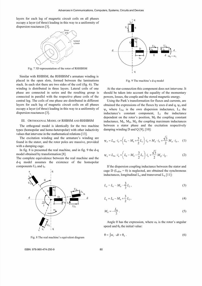
Fig. 7 3D representation of the rotor of RHHBSM

Similar with RHBSM, the RHHBSM’s armature winding is

placed in the open slots, formed between the laminations

stack. In each slot there are two sides of the coil (fig. 6). The

winding is distributed in three layers. Lateral coils of one

phase are connected in series and the resulting group is

connected in parallel with the respective phase coils of the

central leg. The coils of one phase are distributed in differentlayers for each leg of magnetic circuit coils on all phases

occupy a layer (of three) leading in this way to a uniformity of

dispersion reactances [3].

III. ORTHOGONAL MODEL OF RHBSM AND RHHBSM

The orthogonal model is identically for the two machine

types (homopolar and homo-heteropolar) with other inductivity

values that intervene in the mathematical relations [13].

The excitation winding and the armature’s winding are

found in the stator, and the rotor poles are massive, provided

with a damping cage.

In fig. 8 is presented the real machine, and in fig. 9 the d-qmodel obtained by transformation [8].

The complete equivalence between the real machine and the

d-q model assumes the existence of the homopolar

components U0 and i0.

q

q c i C

U C

U a

ia

a

θ

Q ib

iQ

i D

D

U b

U E

b

d d

ω r

3 2 π iE

Fig. 8 The real machine’s equivalent diagram

U q

d

i q q

q

Q i Q

D

i D

U E

i E

U d

i d E d ω b = ω 1

d

q

Fig. 9 The machine’s d-q model

At the star-connection this component does not intervene. It

should be taken into account the equality of the momentary

powers, losses, the couple and the stored magnetic energy.

Using the Park’s transformation for fluxes and currents, areobtained the expressions of the fluxes by axes d and q, ψd and

ψq where LSσ is the own dispersion inductance, L0 the

inductance’s constant component, L2 the inductance

dependent on the rotor’s position, M0 the coupling constant

inductance, ME, MD, MQ the coupling maximum inductances

between a stator phase and the excitation respectively

damping winding D and Q [9], [10]:

DDE E d d S d iM iM iLM LiL ⋅+⋅+⋅⎟⎠

⎞⎜⎝

⎛ +−+⋅=ψ σ2

3

2

3200

, (1)

QQqqS q iM iLM LiL ⋅+⋅⎟⎠

⎞⎜⎝

⎛ −−+⋅=ψ σ

2

3

2

3200 . (2)

If the dispersion coupling inductance between the stator and

cage D (LdDσ = 0) is neglected, are obtained the synchronous

inductances, longitudinal Ld and transversal Lq [11]:

2002

3LM LLd −−= , (3)

200 2

3LM LL

q

+−= , (4)

2

00

LM −= . (5)

Angle θ has the expression, where ωr is the rotor’s angular

speed and θ0 the initial value:

∫ θ+⋅ω=θ 0dt r . (6)


ISBN: 978-960-474-250-9 80



The binding relation between the orthogonal model’s

currents id, iq and i0 and the real machine’s currents ia, ib and ic

is [9]:

[ ]⎥⎥⎥

⎦

⎤

⎢⎢⎢

⎣

⎡

⋅=⎥⎥⎥

⎦

⎤

⎢⎢⎢

⎣

⎡

c

b

a

abcdqq

d

i

i

i

P

i

i

i

0

0

, (7)

where:

2 2cos( ) cos( ) cos( )

3 3

2 2 2sin( ) sin( ) sin( )

3 3 3

1 1 1

2 2 2

abcdqP

π π θ θ θ

π π θ θ θ

⎡ ⎤+ −⎢ ⎥

⎢ ⎥⎢ ⎥⎡ ⎤ = + −⎣ ⎦ ⎢ ⎥⎢ ⎥⎢ ⎥⎢ ⎥⎣ ⎦

, (8)

the same relation being valid also for fluxes,

[ ]⎥⎥⎥

⎦

⎤

⎢⎢⎢

⎣

⎡

ψ

ψ

ψ

⋅=⎥⎥⎥

⎦

⎤

⎢⎢⎢

⎣

⎡

ψ

ψ

ψ

c

b

a

abcdqq

d

P 0

0

. (9)

From the previous relations and taking into account the

relation:

[ ]⎥⎥⎥

⎦

⎤

⎢⎢⎢

⎣

⎡

⋅=⎥⎥⎥

⎦

⎤

⎢⎢⎢

⎣

⎡

0

0

i

i

i

P

i

i

i

q

d

T

abcdq

c

b

a

, (10)

is obtained:

( ) DDE E d S d iM iM iLLL ⋅+⋅+⋅⎥⎦

⎤⎢⎣

⎡++=ψ σ

2

3

2

320 , (11)

( ) QQqS q iM iLLL ⋅+⋅⎥⎦

⎤⎢⎣

⎡−+=ψ σ

2

3

2

320 , (12)

[ ] 00000 2 iLiM LL S S ⋅≅⋅++=ψ σσ . (13)

Considering a single rotor cage by each axis, the voltages

UD = UQ = 0 and the brushes’ speed ωb = ωr , there are

obtained the general equations of the orthogonal model of the

homo-heteropolar synchronous machine, where R S is the

stator resistance, R E the excitation’s resistance, R D and R Q the

rotor cages’ resistances, Me the electromagnetic torque and p

the number of pole pairs:

qr d

d S d t

U Ri ψ⋅ω+∂

ψ∂−=− , (14)

d r

q

qS qt

U Ri ψ⋅ω+∂

ψ∂−=− , (15)

qr E

E E E t

U Ri ψ⋅ω+∂ψ∂

−=− , (16)

t

Ri DDD

∂

ψ∂−= , (17)

t Ri

Q

QQ ∂

ψ∂−= , (18)

( )d qqd e iipM ⋅ψ−⋅ψ= . (19)

IV. THE SPACE-PHASOR MODEL

We define the stator current space-phasor, si in stator

coordinates [14]:

( )cba

s

s iaiaii ⋅+⋅+⋅=2

3

2. (20)

For distributed windings (q ≥ 2) all the stator- self (Laa),

mutual (Lad, Lac, Laf ), and stator-rotor inductances (Ladr , Laqn)

are dependent of the rotor position θer , and rotor inductances

are independent of this.

The phase a flux linkage λa is:

r qr aqr d r ad f af cacbabaaaa iLiLiLiLiLiL +++++=λ . (21)

Making use of the inductance definition we find:

( ) ( ) ( )

( ) ( ) ( )er j

r qr

r sq

er jr

r d r sd er j*

f af

er j*ssssl a

eijLReeiReLeiReL

eiReLiReLiReL

θθθ

θ

−++

+++=λ

2

2

20

2

3

2

3

2

3

. (22)

The stator flux space-phasor λ s is:

( )cba

ss aa λ+λ+λ=λ 2

3

2, (23)

where λb, λc are similar as in (21).

The stator and rotor equation in d-q coordinates becomes[14]:

,dt

d ir V qr

d d sd λω−

λ+⋅= (24)

d r

q

qsqdt

d ir V λω+

λ+⋅= , (25)

,iL ;dt

d ir V f fl f qr

f

f f f ⋅=λλ⋅ω−λ

+⋅= (26)


ISBN: 978-960-474-250-9 81



dmr d l r d r d r d

r d r d iL ;dt

d ir λ+⋅=λ

λ+⋅=0 , (27)

qmr ql r qr qr q

r qr q iL ;dt

d ir λ+⋅=λ

λ+⋅=0 . (28)

The torque Te is [14]:

( ) ( )d qqd

*sse iipijRepT ⋅λ−⋅λ=⋅λ=

2

3

2

3. (29)

Finally, the d-q variables are related to the abc variables by

the Park transformation:

( ) 322

3

2 / jer j

cbaqd s ea ;eV aaV V jV V V π⋅θ− =⋅++=+= . (30)

Note also that all rotor variables are reduced to the stator:

22

d

r drl

drl

d

r dr

dr K

LL ;

K

r r == , (31)

22

q

r

qrl

qrl

q

r

qr

qr K

LL ;

K

r r == . (32)

The equations obtained based on the orthogonal model and

the one of the spatial phasors lead us to the idea that the

second model is more complete, therefore we’ll use it for

designing the control system.

V. CONTROL ALGORITHMS’ DEVELOPMENT

The operation of the RHBSM and RHHBSM synchronous

machines as generator or servomotor with variable speed

presents a special importance at conceiving the adjustment

system’s structure. Based on the spatial phasors’ theory, this

system should be treated unitary. The used model takes in

consideration also the machines’ saturation [15].

A. Basic Control

Scalar control (V / f) is related to sinusoidal current control

without motion sensors (sensorless) (fig. 10) [14]:

RHBSM

(RHHBSM)

DC – DC

Converter

Int.

ControlPI

Control

if

Vref -

+

if

ifref

- +

+

Fig. 10 Scalar control for RHBSM (RHHBSM) with torque angle

increment compensation

For faster dynamics applications, vector control is used (fig.

11) [11], [14].

Speedcontroller

e er PWM generator

PWM inverter

Vd

Positionand speedestimation

i a ib

Va Vbi a i b

θr

p1/s

a

b

a

er

referencespeed

θ

r *

-

i

id

*

*

qi*

a

i*b

i*c r

measuredor estimated

measured or estimated

encoder

DC – DCConverter

Int.Control

PI

Controlif

ω

ω

θ

i d

id*

RHBSM (RHHBSM)

if

ifref

+ -

Fig. 11 Basic vector control of RHBSM (RHHBSM)

a - with encoder; b – without encoder

B. Torque Vector Control

To simplify the motor control, the direct torque and flux

control (DTFC for induction machines) has been extended to

RHBSM (and to RHHBSM) as torque vector control (TVC).Again, fast flux and torque control may be obtained even in

sensorless drive (fig. 12) [11], [14], [15]:

Speedcontroller Commutation

table V (T)

PWM inverter

Vd

Flux, torqueobserver

and speedobserver

ia ib

Va Vb

r

p

1/s

b

a

referencespeed

r *

-

T

s

*

*

e

r

encoder

i

r ^

Te^

s^

-

-

α

DC – DC

Converter

Int.

ControlPI

Controlif id

id*

RHBSM (RHHBSM)

Ref

transf

Int.

Control

ωω

ω

θ

θλs

λ

λ

if

ifref

- +

Fig. 12 Torque vector control (TVC) of RHBSM (RHHBSM)

a - with encoder; b – without encoder

C. Simulation Results

The voltage source inverter used in simulations was a

Danfoss VLT 3005, 5 KVA one, working at 7 KHz switching

frequency. The RHBSM has the following parameters: PN =

2.5 kW, UN = 400 V, Y, IN = 5.5 A, f N = 50 Hz, p = 3, R s = 2

Ω, Ld = 0.023 H, Lq = 0.017 H, IEN = 6 A.

Further, the simulation results are presented with sensorless

control of RHBSM at different speeds and during transients

(speed step response and speed reversing) using DTC and

SVM control strategies [14].

To eliminate the nonlinear effects produced by the inverter,

the dead time compensation is 2.5 μs.

Steady state performance of RHBSM drive with DTFC

control strategy at 25 rpm is presented in figure 13 (in “a” is

represented estimated torque and in “b” the estimated speed).


ISBN: 978-960-474-250-9 82



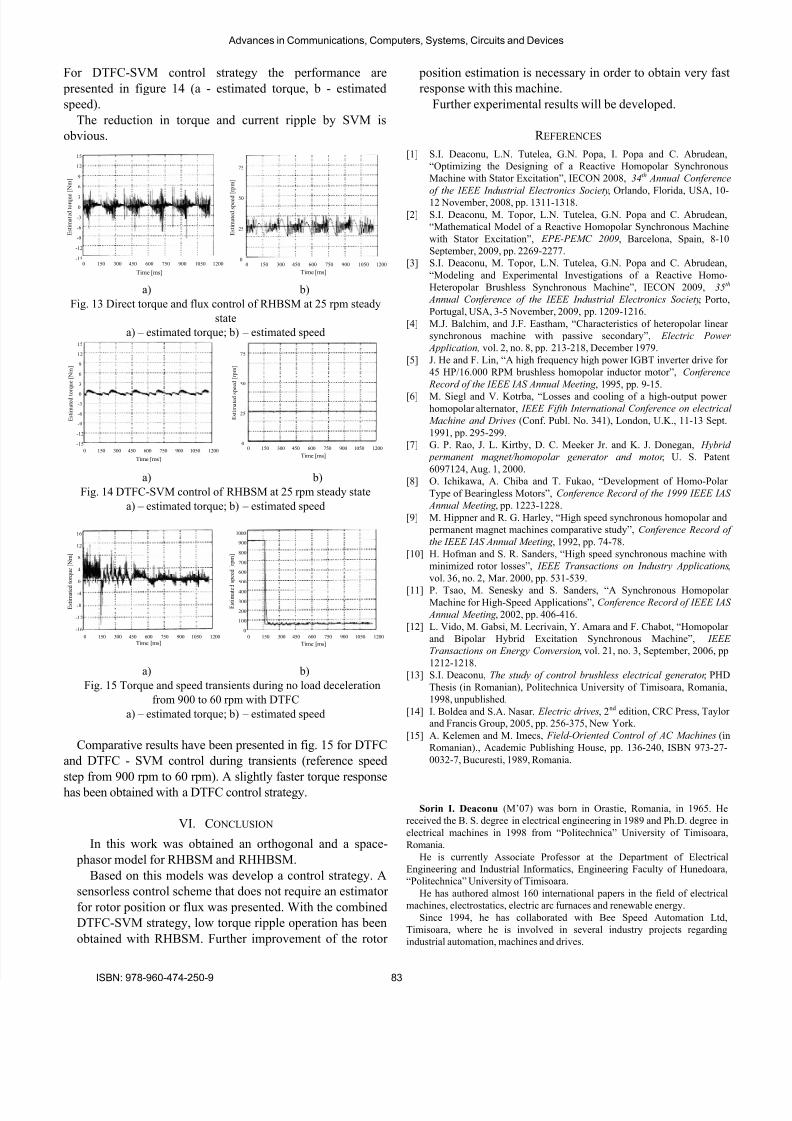
For DTFC-SVM control strategy the performance are

presented in figure 14 (a - estimated torque, b - estimated

speed).

The reduction in torque and current ripple by SVM is

obvious.

15

12

9

6

3

0

-3

-6

-9

-12

-15

Estimated torque

[Nm]

0 150 300 450 600 750 900 1050 1200

Time [ms]

0 150 300 450 600 750 900 1050 1200

Time [ms]

75

50

25

0

Estimated speed [rpm]

a) b)

Fig. 13 Direct torque and flux control of RHBSM at 25 rpm steady

state

a) – estimated torque; b) – estimated speed15

12

9

6

3

0

-3

-6

-9

-12

-15

Estimated to

rque [Nm]

0 150 300 450 600 750 900 1050 1200

Time [ms]

0 150 300 450 600 750 900 1050 1200

Time [ms]

75

50

25

0

Estimated speed [rpm]

a) b)

Fig. 14 DTFC-SVM control of RHBSM at 25 rpm steady state

a) – estimated torque; b) – estimated speed

16

12

8

4

0

-4

-8

-12

-16

0 150 300 450 600 750 900 1050 1200

Time [ms]

Estimated torque [Nm]

1000

900

800

700

600

500

400

300

200

100

0

0 150 300 450 600 750 900 1050 1200

Time [ms]

Estimate

d speed [rpm]

a) b)

Fig. 15 Torque and speed transients during no load deceleration

from 900 to 60 rpm with DTFC

a) – estimated torque; b) – estimated speed

Comparative results have been presented in fig. 15 for DTFC

and DTFC - SVM control during transients (reference speed

step from 900 rpm to 60 rpm). A slightly faster torque response

has been obtained with a DTFC control strategy.

VI. CONCLUSION

In this work was obtained an orthogonal and a space-

phasor model for RHBSM and RHHBSM.

Based on this models was develop a control strategy. A

sensorless control scheme that does not require an estimator

for rotor position or flux was presented. With the combined

DTFC-SVM strategy, low torque ripple operation has been

obtained with RHBSM. Further improvement of the rotor

position estimation is necessary in order to obtain very fast

response with this machine.

Further experimental results will be developed.

R EFERENCES

[1] S.I. Deaconu, L.N. Tutelea, G.N. Popa, I. Popa and C. Abrudean,

“Optimizing the Designing of a Reactive Homopolar Synchronous

Machine with Stator Excitation”, IECON 2008, 34th Annual Conference

of the IEEE Industrial Electronics Society, Orlando, Florida, USA, 10-

12 November, 2008, pp. 1311-1318.

[2] S.I. Deaconu, M. Topor, L.N. Tutelea, G.N. Popa and C. Abrudean,

“Mathematical Model of a Reactive Homopolar Synchronous Machine

with Stator Excitation”, EPE-PEMC 2009, Barcelona, Spain, 8-10

September, 2009, pp. 2269-2277.

[3] S.I. Deaconu, M. Topor, L.N. Tutelea, G.N. Popa and C. Abrudean,

“Modeling and Experimental Investigations of a Reactive Homo-

Heteropolar Brushless Synchronous Machine”, IECON 2009, 35th

Annual Conference of the IEEE Industrial Electronics Society, Porto,

Portugal, USA, 3-5 November, 2009, pp. 1209-1216.

[4] M.J. Balchim, and J.F. Eastham, “Characteristics of heteropolar linear

synchronous machine with passive secondary”, Electric Power

Application, vol. 2, no. 8, pp. 213-218, December 1979.

[5] J. He and F. Lin, “A high frequency high power IGBT inverter drive for

45 HP/16.000 RPM brushless homopolar inductor motor”, Conference

Record of the IEEE IAS Annual Meeting , 1995, pp. 9-15.

[6] M. Siegl and V. Kotrba, “Losses and cooling of a high-output power

homopolar alternator, IEEE Fifth International Conference on electrical

Machine and Drives (Conf. Publ. No. 341), London, U.K., 11-13 Sept.

1991, pp. 295-299.

[7] G. P. Rao, J. L. Kirtby, D. C. Meeker Jr. and K. J. Donegan, Hybrid

permanent magnet/homopolar generator and motor , U. S. Patent

6097124, Aug. 1, 2000.

[8] O. Ichikawa, A. Chiba and T. Fukao, “Development of Homo-Polar

Type of Bearingless Motors”, Conference Record of the 1999 IEEE IAS

Annual Meeting , pp. 1223-1228.

[9] M. Hippner and R. G. Harley, “High speed synchronous homopolar and

permanent magnet machines comparative study”, Conference Record of

the IEEE IAS Annual Meeting , 1992, pp. 74-78.

[10] H. Hofman and S. R. Sanders, “High speed synchronous machine with

minimized rotor losses”, IEEE Transactions on Industry Applications,

vol. 36, no. 2, Mar. 2000, pp. 531-539.

[11] P. Tsao, M. Senesky and S. Sanders, “A Synchronous Homopolar Machine for High-Speed Applications”, Conference Record of IEEE IAS

Annual Meeting , 2002, pp. 406-416.

[12] L. Vido, M. Gabsi, M. Lecrivain, Y. Amara and F. Chabot, “Homopolar

and Bipolar Hybrid Excitation Synchronous Machine”, IEEE

Transactions on Energy Conversion, vol. 21, no. 3, September, 2006, pp

1212-1218.

[13] S.I. Deaconu, The study of control brushless electrical generator , PHD

Thesis (in Romanian), Politechnica University of Timisoara, Romania,

1998, unpublished.

[14] I. Boldea and S.A. Nasar, Electric drives, 2nd edition, CRC Press, Taylor

and Francis Group, 2005, pp. 256-375, New York.

[15] A. Kelemen and M. Imecs, Field-Oriented Control of AC Machines (in

Romanian)., Academic Publishing House, pp. 136-240, ISBN 973-27-

0032-7, Bucuresti, 1989, Romania.

Sorin I. Deaconu (M’07) was born in Orastie, Romania, in 1965. He

received the B. S. degree in electrical engineering in 1989 and Ph.D. degree in

electrical machines in 1998 from “Politechnica” University of Timisoara,

Romania.

He is currently Associate Professor at the Department of Electrical

Engineering and Industrial Informatics, Engineering Faculty of Hunedoara,

“Politechnica” University of Timisoara.

He has authored almost 160 international papers in the field of electrical

machines, electrostatics, electric arc furnaces and renewable energy.

Since 1994, he has collaborated with Bee Speed Automation Ltd,

Timisoara, where he is involved in several industry projects regarding

industrial automation, machines and drives.


ISBN: 978-960-474-250-9 83

cscc-13 rad sa sorinom

Documents