csc494: individual project in computer sciencekamyar/documents/csc494_project_report.pdf · csc494:...

CSC494: Individual Project in Computer Science

Seyed Kamyar Seyed GhasemipourDepartment of Computer Science

University of [email protected]

Abstract

One of the most important tasks in computer vision isobject recognition. In this work we explore to what extentlocal descriptors computed at keypoints can be useful forthis task. We experiment with different combinations of key-point detectors and local feature descriptors on a dataset ofpoint clouds of rendered CAD models as well as a datasetof point clouds of individual object instances segmented outfrom RGB-D images of natural scenes. Our results demon-strate that by jointly taking into account the features com-puted from an object, a simple nearest neighbour classifica-tion framework can result in interesting classification per-formance.

1. IntroductionOne of the most important components of an object

recognition pipeline is the representations of the objects thatare used. The most successful methods in this area itera-tively build more complex, higher order representations bycombining lower order ones to create more semantic repre-sentations. In this report, on the other hand, we explore theefficacy of using purely local feature descriptors, extractedat specific interest points, for the task of object recognition.

fiIn the task of recognizing a specific object instanceacross multiple scenes, in the presence of clutter, and withvariations in viewpoint, a standard pipeline is to employ akeypoint detection algorithm to find salient, repeatable in-terest points on the object, and then proceed to encode, in asufficiently unique manner, the detected interest points andtheir surrounding neighborhoods using a feature descriptor.At test time, given a novel scene, the features of the objectsof interest are compared against features which were ex-tracted from the scene in a similar manner. Given sufficientconsensus between the relative locations of the matched fea-tures in the scene and the ones on a previously seen object,the object is noted to have been discovered in the scene.

In this work, we explore to what extent this pipeline canbe used for object recognition. We experiment with combi-

nations of two keypoint detectors and two feature descrip-tors on two different datasets: a dataset of point clouds gen-erated from CAD models of 10 common household objects,and a dataset of point clouds of the same object classes ex-tracted from natural indoor scenes.

2. Datasets

As mentioned above, we experiment with artificial aswell as natural data. This allows us to more effectively ana-lyze the ability of our approach; the artificial set provides an“easy”, noiseless benchmark for testing our method and thenatural, noisy set gauges transferability to real-world sce-narios.

Both datasets consist of point clouds of individual objectinstances from 10 classes of household objects. The objectsconsidered in our experiments are: bathtub, bed, chair, desk,dresser, monitor, night stand, sofa, table, and toilet. Weproceed to briefly describe the method of generation of eachdataset.

2.1. Artificial Data

To generate our artificial data, we made use of a collec-tion of CAD models (of objects from the aforementionedclasses) gathered by Wu et al. [7]. To simulate having a2.5D point cloud, given each CAD model, a uniform gridof 12 points was placed on a sphere centered at the givenobject [8]. Subsequently, the object was rendered from theviewpoint of cameras placed on the grid points, looking to-wards the center of the sphere. The depth buffer of each ofthe renderings was then converted to a point cloud to gen-erate our artificial dataset. In our experiments with the ar-tificial data, we test our object recognition method for twoscenarios: recognizing previously seen objects from novelviewpoints and recognizing novel object instances. For thepurposes of our experiments, we created three data splits:

• Train Set: To create the training split, for each objectclass 20 instances were chosen, and for each instance,4 of the 12 views were picked at random.

1

• New Views Test Set: This set was created by ran-domly choosing 2 other views for the instances in thetraining set.

• Novel Objects Test Set: The test set of novel objectinstances was created by randomly choosing 4 of 12views for 5 different instances of each object category.

2.2. Natural Data

In our experiments, we also made use of the NYU DepthDataset V2 [2]. This dataset consists of RGB-D images ofvarious indoor scenes, with instance-level segmentations ofthe objects in the images. Using these segmentation anno-tations, we separated out instances of the objects of interestfrom the images and converted them into point clouds. Thetrain and test sets for experiments with natural data con-tained 12 and 3 instances per object category respectively.

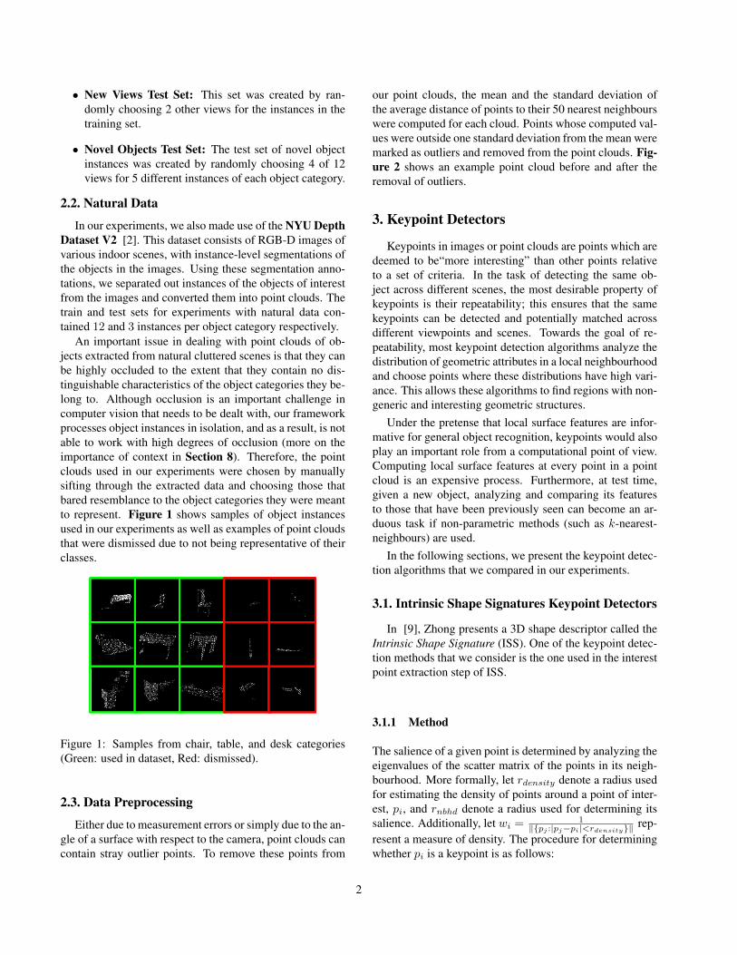
An important issue in dealing with point clouds of ob-jects extracted from natural cluttered scenes is that they canbe highly occluded to the extent that they contain no dis-tinguishable characteristics of the object categories they be-long to. Although occlusion is an important challenge incomputer vision that needs to be dealt with, our frameworkprocesses object instances in isolation, and as a result, is notable to work with high degrees of occlusion (more on theimportance of context in Section 8). Therefore, the pointclouds used in our experiments were chosen by manuallysifting through the extracted data and choosing those thatbared resemblance to the object categories they were meantto represent. Figure 1 shows samples of object instancesused in our experiments as well as examples of point cloudsthat were dismissed due to not being representative of theirclasses.

Figure 1: Samples from chair, table, and desk categories(Green: used in dataset, Red: dismissed).

2.3. Data Preprocessing

Either due to measurement errors or simply due to the an-gle of a surface with respect to the camera, point clouds cancontain stray outlier points. To remove these points from

our point clouds, the mean and the standard deviation ofthe average distance of points to their 50 nearest neighbourswere computed for each cloud. Points whose computed val-ues were outside one standard deviation from the mean weremarked as outliers and removed from the point clouds. Fig-ure 2 shows an example point cloud before and after theremoval of outliers.

3. Keypoint Detectors

Keypoints in images or point clouds are points which aredeemed to be“more interesting” than other points relativeto a set of criteria. In the task of detecting the same ob-ject across different scenes, the most desirable property ofkeypoints is their repeatability; this ensures that the samekeypoints can be detected and potentially matched acrossdifferent viewpoints and scenes. Towards the goal of re-peatability, most keypoint detection algorithms analyze thedistribution of geometric attributes in a local neighbourhoodand choose points where these distributions have high vari-ance. This allows these algorithms to find regions with non-generic and interesting geometric structures.

Under the pretense that local surface features are infor-mative for general object recognition, keypoints would alsoplay an important role from a computational point of view.Computing local surface features at every point in a pointcloud is an expensive process. Furthermore, at test time,given a new object, analyzing and comparing its featuresto those that have been previously seen can become an ar-duous task if non-parametric methods (such as k-nearest-neighbours) are used.

In the following sections, we present the keypoint detec-tion algorithms that we compared in our experiments.

3.1. Intrinsic Shape Signatures Keypoint Detectors

In [9], Zhong presents a 3D shape descriptor called theIntrinsic Shape Signature (ISS). One of the keypoint detec-tion methods that we consider is the one used in the interestpoint extraction step of ISS.

3.1.1 Method

The salience of a given point is determined by analyzing theeigenvalues of the scatter matrix of the points in its neigh-bourhood. More formally, let rdensity denote a radius usedfor estimating the density of points around a point of inter-est, pi, and rnbhd denote a radius used for determining itssalience. Additionally, let wi = 1

‖{pj :|pj−pi|<rdensity}‖ rep-resent a measure of density. The procedure for determiningwhether pi is a keypoint is as follows:

2

Figure 2: An example point cloud before and after outlier removal.

1. The weighted scatter matrix about pi is computed as:

SC(pi) =∑

|pj−pi|<rnbhd

wj(pj − pi)(pj − pi)T∑|pj−pi|<rnbhd

wj

2. The eigenvalues of SC(pi) are computed next. λ1i ,λ2i , λ3i represent the eigenvalues in order of decreas-ing magnitude.

3. Points where λ2i

λ1i< γ21 and λ3

i

λ2i< γ32 are chosen as the

potential set of keypoints (γ21 and γ32 are parametersthat can be tuned).

4. The final set of keypoints are determined by non-maximal suppression using the magnitude of λ3i .

3.1.2 Intuition

The eigenvalues of SC(pi) represent to what extent the po-sitions of points in the local pi neighbourhood vary alongthree orthogonal axes. Therefore the behaviour or the key-point detection method outlined above depends heavily onthe values of γ21 and γ32.

If γ21 and γ32 are both large, then all points pass throughstep 3, and the resulting set of keypoints will contain pointswhose neighbours are scattered in every direction. How-ever, on flat surfaces, such as the bottom of a chair, themagnitude of the third eigenvector is very small in com-parison to the first two. In such regions, as a result of thenon-maximal suppression step, the algorithm will behavesimilarly to uniform sampling of points.

Setting γ21 and γ32 to be too small also have side-effects.If γ32 is small, the keypoints will capture flat surfaces whichis not a desirable property. However, making γ21 small willhelp to capture edges since at a point on a 3-dimensionaledge, there will typically be two directions with neighbourson only one side, and a third direction with neighbours onboth sides of the points.

Lastly, we observe that it would be difficult for thismethod to detect corners. At corners, all three eigenval-ues would have similar magnitudes. Therefore, unless γ21and γ32 are both set to be large, corners will not be detectedas keypoints. Indeed, the first image in Figure 3 shows thatsetting γ21 and γ32 to 0.7 and 0.5 respectively, the algorithmdid not choose the corners of the table as keypoints.

3.2. Harris 3D Corner Detector

The Harris corner detector is a popular method of ex-tracting interest points from 2D images. One of the keypointdetectors that we use in our experiments is the extension ofthe Harris corner detector to 3D point clouds.

3.2.1 Method

Let I(j)x and I(j)y denote the gradients in the x and y direc-tions at the point pi in a 2D image. In the original Harriscorner detection algorithm, the magnitude of the eigenval-ues of:

M(pi) =∑

|pj−pi|<rnbhd

[I(j)x , I(j)y ][I(j)x , I(j)y ]T

are considered to be indicative of the existence of an edgeor corner at pi.

The extension of this idea to the case of 3D point clouds,as implemented in the Point Cloud Library (PCL) [4] is toreplace the matrix M with the covariance of the normals atthe points in the neighbourhood of pi:

COV (pi) =∑

|pj−pi|<rdensity

Nj ·NTj

3.2.2 Intuition

The method described in 3.1 cares about the spatial distri-bution of points in a local neighbourhood. However, thisinformation does not say much about the curvature of the

3

Figure 3: Keypoints detected on a table (left: ISS, right: Harris).

Figure 4: Keypoints detected on a chair using different methods (in order from left to right: ISS, Harris, Uniform).

local region. On the other hand, the Harris 3D corner detec-tor does consider this information by caring about to whatextent the direction of the surface normals vary along dif-ferent orthogonal directions. A comparison of keypointsdetected with the two methods discussed thus far can beseen in Figures 3 and 4

3.3. Uniform Sampling

As mentioned before, keypoint detection methods tendto care about non-generic regions with interesting struc-tures. However, for building representations of objects, highvariance regions are not the only informative regions. Theexistence and the distribution of smooth and flat regionscould also be valuable information. Hence, as a baselineto the two keypoint detection techniques mentioned above,we also experiment with uniformly sampling points fromour point clouds as a replacement for interest point detec-tion algorithms.

3.4. Practical Notes & Implementation Details

Two important parameters that need to be set for thecomputation of ISS keypoints are rnbhd and the radius ofnon-maxima suppression. Data from our point clouds cancontain a significant amount of noise (this is especially true

for natural data). Therefore, we would not want these radiito be too small. After some parameter tuning, we decidedto set rnbhd and the radius of non-maximal suppression tobe respectively 12 and 8 times the model resolution, wherethe model resolution of a point cloud is computed as theaverage distance of a point to its nearest neighbour in thecloud.

For the Harris keypoint detector, we set the radius usedfor performing the computations to be 8 times the modelresolution. Additionally, this detector also requires surfacenormals to be computed. If the support radius used to com-pute the normals is too small, the computations will be sus-ceptible to noise. On the other hand, if this radius is toolarge, the normals inside a local region will be very simi-lar to one another, thereby negatively affecting the keypointdetection process. Eventually, we decided to set this param-eter to be 3 times the model resolution.

For uniform sampling, we randomly sampled 2625 points

from the point cloud for each object.

3.5. Statistics

The table below presents the mean ratio of number ofkeypoints detected to the number of points in the pointclouds for objects in the training sets of each dataset. The

4

Dataset ISS Harris 3D UniformNatural Data 0.0048 0.0043 0.0031

Artificial Data 0.0027 0.0036 0.0032

Table 1: Ratio of keypoints to number of points in pointcloud.

larger ratios for the natural dataset is a result of the noisiernature of the data.

4. Local Descriptors

After performing keypoint extraction from the data of in-terest, the next step in our experimental pipeline is to com-pute local descriptors at the salient points. The role of a de-scriptor computed at a given point is to represent the prop-erties of the local surface around the point in a compact, yetsufficiently unique manner. Below, we discuss two localdescriptors that we used in our experiments.

4.1. Fast Point Feature Histograms

In [5], Rusu et al. present the Point Feature Histogram(PFH) as means of capturing the geometrical properties ofthe neighbourhood of a point. In later work, [3], presents amodification of PFH named Fast Point Feature Histogram(FPFH) which significantly reduces the computational costassociated with the feature computation. We proceed byfirst describing the how PFH are computed and explain howit has been modified to produce the FPFH.

4.1.1 Point Feature Histograms

Point Feature Histograms attempt to capture the geometryof a local region by taking into account the relative directionof the normals in that region. Given a point of interest, pq ,the PFH for that point is computed as follows:

1. Let S(pq) = {pt : |pq − pt| < rnbhd} where rnbhd isa hyperparameter of the feature computation.

2. For a given pair of points (ps, pt) in S(pq), withnormals (ns, nt), the point whose normal makes thesmallest angle with ps − pt is chosen as the source.

3. Without loss of generality, we assume the source to beps. A frame about the point ps is created using theorthonormal basis (u, v, w) defined as follows:

u = ns

v =(pt − ps)|pt − ps|

w = u× v

Figure 5: Visualization of local frame and angles used forthe computation of Point Feature Histograms [1].

4. Given this frame, the quadruplet 〈α, φ, θ, d〉 for thepair (ps, pt) is formed where:

d = |pt − ps|α = v · nt

φ = u · (pt − ps)d

θ = arctan(w · nt, u · nt)

5. For 2.5D images, however, the distance betweenneighbouring points differs across viewpoints. There-fore, it is common to eliminate the d element from thequadruplet. To create the PFH descriptor for the pointpq , the triplets 〈α, φ, θ〉 are computed for every pair ofpoints in S(pq). α, φ, and θ are each binned using 5bins, creating a total of 53 bins for the triplets. ThePoint Feature Histogram for pq is then taken to be the125-dimensional histogram of the computed triplets.

4.1.2 Fast Point Feature Histograms

Computing Point Feature Histograms incurs a high compu-tational cost due to the fact that the mentioned triplets arecomputed for every pair of points in the neighbourhood ofthe point we are considering. The Fast Point Feature His-togram [3] attempts to remedy this issue as follows:

1. In the first step, Simplified Point Feature Histograms(SPFH) are computed at every point in the cloud. Fora given point pq , SPFH is computed in a very similarmanner as PFH with 2 main differences:

• The triplets 〈α, φ, θ〉 are only computed betweenpq and its neighbours.

• Instead of jointly binning the values of thetriplets, a histogram of 11 bins is made foreach of α, φ, and θ separately, and the resul-tant histograms are concatenated to form a 33-dimensional feature vector.

5

2. In the second step, the FPFH feature for point pq iscomputed to be:

FPFH(pq) = SPFH(pq)

+1

‖ S(pq) ‖∑

pk∈S(pq)

1

wk· SPFH(pk)

where wk is the distance of pq to pk.

4.1.3 Intuitions

FPFH attempts to capture the geometry of a local region bymeasuring how the direction of the normals in the regionchange relative to one another. However, without informa-tion about the relative location of the normals, the same de-scriptor could potentially represent many types of surfacegeometries. This, in addition to the fact that α, φ, and θare binned independently raises a concern about how dis-tinctive FPFH features are in terms of representing surfaceswith different structures.

On a positive note however, the fact that FPFH featuresonly consider the relative directions of normals means thatFPFH features are pose invariant and should in theory pro-duce the same histograms when objects are seen from dif-ferent viewpoints.

4.2. SHOT Descriptor

In [6], Tombari et al. present the Signature of His-tograms of Orientations (SHOT). This is the second de-scriptor that we employed in our experiments.

4.2.1 Method

To compute the descriptor at a point pi, the SHOT descriptorfirst necessitates the computation of a local reference frame.This reference frame is computed at follows:

1. Let M be:

M =

∑j:dj≤rnbhd

(rnbhd − dj)(pi − pj)(pi − pj)T∑j:dj≤rnbhd

(rnbhd − dj)

where rnbhd is a hand tuned parameter.

2. The directions of the eigenvectors sorted in decreasingorder of eigenvalue magnitude are taken in order to bethe directions of the x, y, and z axes of the local ref-erence frame. We will denote these eigenvectors withx, y, z.

3. Let S+x = {j : dj < rnbhd ∧ (pj − p) · x ≥ 0} and

S−x = {j : dj < rnbhd ∧ (pj − p) · (−x) > 0}. Thepositive direction of the x axis for the reference frames

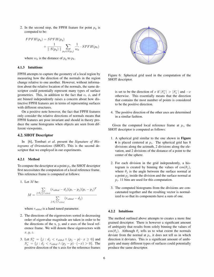
Figure 6: Spherical grid used in the computation of theSHOT descriptor.

is set to be the direction of x if |S+x | > |S−x | and −x

otherwise. This essentially means that the directionthat contains the most number of points is consideredto be the positive direction.

4. The positive direction of the other axes are determinedin a similar fashion.

Given the computed local reference frame at pi, theSHOT descriptor is computed as follows:

1. A spherical grid similar to the one shown in Figure6 is placed centered at pi. The spherical grid has 8divisions along the azimuth, 2 divisions along the ele-vation, and 2 divisions of the distance of a point to thecenter of the sphere.

2. For each division in the grid independently, a his-togram is created by binning the values of cos(θj),where θj is the angle between the surface normal ata point pj inside the division and the surface normal atpi. 11 bins are used for this computation.

3. The computed histograms from the divisions are con-catenated together and the resulting vector is normal-ized to so that its components have a sum of one.

4.2.2 Intuitions

The method outlined above attempts to creates a more finegrained descriptor. There is however a significant amountof ambiguity that results from solely binning the values ofcos(θj). Although θj tells us to what extent the normalsdeviate from the normal at pi, it does not tell us in whichdirection it deviates. This is a significant amount of ambi-guity and many different types of surfaces could potentiallyproduce the same descriptor.

6

4.3. Practical Notes & Implementation Details

To use the local descriptors for the purpose of objectrecognition, we decided to choose a not so small value forrnbhd so as to capture the geometry of a larger region anddeal with the presence of noise. We decided to set this valueto 12 times the resolution of the point clouds. Similar to thecase when detecting keypoints, the support radius for nor-mal computation was set to 3 times the resolution of thepoint clouds.

There also exists a practical issue when working withSHOT descriptors; they are very high dimensional descrip-tors (352 for SHOT vs. 33 for FPFH). This creates a compu-tational problem for performing nearest neighbour queries.To resolve this issue, using PCA, 30 highly informative or-thogonal axes of the SHOT descriptors were identified bylooking at the training set. Subsequently, all SHOT descrip-tors from the training and test sets were preprocessed by be-ing projected onto the derived axes (this was done for eachdataset independently).

5. A Priori Expectations

A priori, we do not expect the method we employ in thiswork to produce amazing results.

To begin with, the features that we extract are local sur-face descriptors. It is quite possible to significantly modifythe local structure of points in a point cloud (for example byadding sufficient amounts of noise) while still preserving aglobal structure that allows for the recognition of the objectby a human, but not by our method. Additionally, in ourframework, we are not taking into account the relative po-sitions of the keypoints at which we extract features. Evenby encoding this information, we would still be required todeal with the ambiguities associated with working with ro-tation invariant feature descriptors.

However, if we observe positive results in our experi-ments, this will indicate that the local features we extractare able to represent non-trivial aspects of the objects theyare derived from, providing motivation for future work toattempt to incorporate this information with more globalproperties in order to build better representations of objects.

6. Experiments

In this section we discuss the experiments we carried outusing our pipeline. As mentioned in section 2, we workedwith both an artificial and a natural dataset. For the arti-ficial dataset we experimented with recognizing previouslyseen objects from new viewpoints in addition to recognizingnovel objects. For the natural dataset however, we only ex-periment with recognizing previously unseen objects fromthe given object categories.

6.1. Distinctiveness of Individual Keypoints

As a first experiment, it would be interesting to exploreto what extent features extracted from objects are indicativeof the class of the object. To this effect, we performed twotests:

6.1.1 k-NN

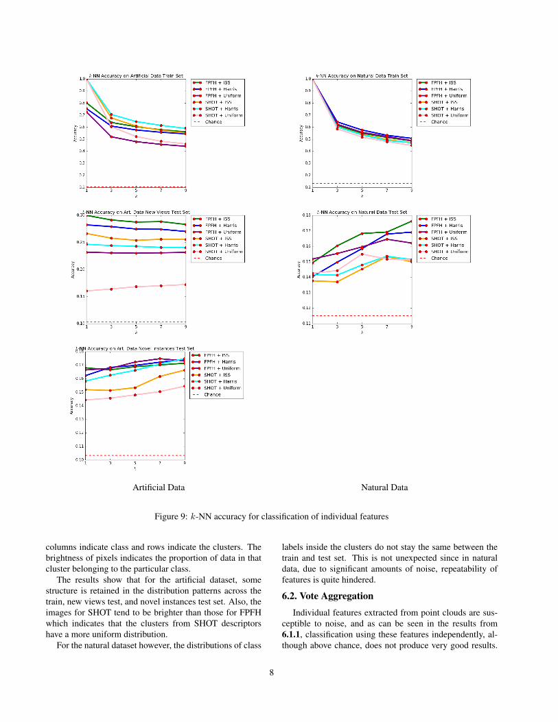
If individual features extracted at keypoints are representa-tive of the object category, nearest neighbours classificationof the features should produce results better than chance.For a given value of k, nearest neighbours classificationwas done by first determining the k nearest neighbours toa query point, q, and creating a voting mechanism in whichthe neighbours vote for their object class using a weight in-versely proportional to their distance from q. The plots inFigure 9 demonstrate the classification accuracy of k-NNfor k ∈ {1, 3, 5, 7, 9} on both datasets for every combina-tion of keypoint extractor and feature descriptor.

First, the fact that we obtain results consistently betterthan chance indicates that there may indeed exist informa-tion that can be leveraged from the local descriptors.

Interestingly, the plot for the new views test set of the ar-tificial data seems to produce a strict ordering of the qualityof the keypoint/descriptor combinations. Since good per-formance on this test set would require the repeatabilityof keypoints and distinctiveness of the descriptors, the re-sults indicate that the ISS keypoints are better repeatablethan Harris corners, and that FPFH features better describethe local surfaces of the objects. On novel object test setsfor both datasets however, “uniform” methods achieve closeperformance to keypoint-based ones and the benefit of hav-ing keypoints diminishes.

Lastly, we note that FPFH based methods do not achieve100% accuracy for 1-NN on the training sets. This is due tothe fact that FPFH features for various points end up havingthe same description. This is related to our previous con-cern regarding the distinctiveness of FPFH but we do notknow how to reconcile this with their superior performancediscussed in the previous paragraph.

6.1.2 k-Means

If the extracted features are indicative of class, after per-forming k-means clustering on the descriptors, the distribu-tion of class labels in each cluster should be non-uniformand heavily skewed. To perform this analysis, for eachdataset, the training set was clustered using k-means clus-tering with 50 clusters. Subsequently, the features from thetest sets were assigned to the cluster with the closest cen-ter. The figures on pages 9 and 10 demonstrate the distribu-tion of class labels inside the clusters for the various combi-nations of keypoints and descriptors. In the visualizations,

7

Artificial Data Natural Data

Figure 9: k-NN accuracy for classification of individual features

columns indicate class and rows indicate the clusters. Thebrightness of pixels indicates the proportion of data in thatcluster belonging to the particular class.

The results show that for the artificial dataset, somestructure is retained in the distribution patterns across thetrain, new views test, and novel instances test set. Also, theimages for SHOT tend to be brighter than those for FPFHwhich indicates that the clusters from SHOT descriptorshave a more uniform distribution.

For the natural dataset however, the distributions of class

labels inside the clusters do not stay the same between thetrain and test set. This is not unexpected since in naturaldata, due to significant amounts of noise, repeatability offeatures is quite hindered.

6.2. Vote Aggregation

Individual features extracted from point clouds are sus-ceptible to noise, and as can be seen in the results from6.1.1, classification using these features independently, al-though above chance, does not produce very good results.

8

FPFH + ISS FPFH + Harris FPFH + Uniform SHOT + ISS SHOT + Harris SHOT + Uniform

Figure 16: Distribution of labels in each of 50 cluster for TRAIN set of ARTIFICIAL DATA.


Figure 23: Distribution of labels in each of 50 cluster for NEW VIEWS TEST set of ARTIFICIAL DATA.


Figure 30: Distribution of labels in each of 50 cluster for NOVEL INSTANCES TEST set of ARTIFICIAL DATA.

In this experiment instead, the individual features of an ob-ject voted for a class determined by the k-NN classifica-tion decision. The majority vote of the predicted classeswas taken as the prediction for the full object. Figure 47presents the results obtained from this experiment.

At first glance, classification performance for the artifi-cial dataset is improved very significantly whereas for nat-ural data, the results are a mix of performance gain and lossfor different types of keypoint-descriptor pairs.

Looking at the results obtained from the various test sets,what is quite odd is that the relative ordering of how well

different keypoint-descriptor combinations perform is notpreserved; for the artificial dataset, the SHOT descriptor isactually doing a better job than FPFH, whereas the case wasthe reverse when classifying individual features. We do nothave a justification for why this may have occurred.

One aspect that is preserved between the results from6.1.1 and here is the fact that keypoint based feature com-putations results in noticeably better accuracies for only the“new views” test set of the artificial dataset, but the per-formance gap shrinks in when working when novel objectinstances are considered.

9


Figure 37: Distribution of labels in each of 50 cluster for TRAIN set of NATURAL DATA.


Figure 44: Distribution of labels in each of 50 cluster for TEST set of NATURAL DATA.

6.3. Histogram of Histograms

The last experiment that we did was to use a global rep-resentation of the objects derived from local feature descrip-tors. The representation that we used was computed as fol-lows:

1. Features from the training set were clustered using k-means clustering with 50 clusters.

2. For objects in both train and test sets, a histogram with50 bins was created where the bins represent the num-ber of features from the given object that belong to agiven cluster.

3. The histograms, normalized so that the values in thebins sum to one, are subsequently used as the repre-sentations of the objects.

Classification using these representations was done in asimilar fashion to experiment 6.1.1 with the difference thathere the data points are the computed histograms. The plotsin Figure 50 present the classification results.

This set of plots shares similar properties to the two pre-vious ones from experiments 6.1.1 and 6.2 (such as the key-points being more relevant to the “new views” test set thanfor the “novel objects” test set) and the performance on the

artificial dataset seems to be in between those of experi-ments 6.1.1 and 6.2. However, the most interesting resultfrom this experiment is that we were able to significantlyimprove classification accuracy on the natural data test set,which we were not able to do in experiment 6.2. This isquite surprising to us since the results from section 6.1.2were hinting that the distribution of prototypical featureswere changing significantly between the natural data trainand test sets (further discussion in conclusions section).

7. Conclusions

In this work, we explored to what extent local descriptorscomputed at keypoints can be useful for object recogntion.We experimented with with FPFH and SHOT descriptorscomputed at keypoints computed using 3 different methods,ISS Keypoints, Harris 3D Corners, and Uniform Sampling.To adapt this framework from instance detection to objectrecognition, we used larger radii of salience to capture in-formation that is less local.

Our experiments show that individual features on theirown do not contain enough information for doing good clas-sification. However, when the predictions for the individ-ual features from an object are combined to make a judge-ment about object class, there is a very significant improve-

10


Figure 47: k-NN accuracy for instance-level classification

ment in performance for the artificial dataset. This, how-ever, does not improve classification accuracy for naturaldata significantly. The reason could be that due to the sig-nificant amount of noise in natural data, keypoint detectiondoes not perform well and descriptors do not represent thetrue surface shape. Additionally, we note that the similarityof accuracies on the “novel objects” artificial test set withor without the use of keypoints (keypoints vs. uniform sam-pling) could indicate that smooth regions are also informa-tive of the class of objects.

Lastly, an interesting result that we observed was thatclassification results for natural data are significantly im-proved in the experiment in section 6.3. The results on arti-ficial data indicated that when considered jointly, the com-puted features can be useful for recognizing the class of anobject. Representing objects using histograms of prototypi-cal features could be considered as also doing the same withthe added benefit of robustness to noise due to substitutingfeatures with their prototypes (cluster centers). Since nat-ural data are noisy, the results on those test sets were im-

11


Figure 50: k-NN accuracy for classification using normalized histogram of prototypical features

proved whereas the results for artificial data were compara-ble to those obtained in experiment 6.2.

8. Future Directions

The work in this report is applicable to a constrained sit-uation. First, we required that object instances be separated.Segmenting out individual objects from cluttered scenes isa very difficult task and if we do not perform the segmenta-tion, our feature computations will be inaccurate. Second,

we only experimented with non-occluded (artificial data) ornot-heavily-occluded (natural data) objects. Self-occlusionwas present in our data however. This will also pose a ma-jor problem for us as our best results were achieved with theaggregation of votes from the features over the entire object.

Another problem with our approach is that we treat ob-jects in isolation. Context is extremely important in helpingwith classification, especially when significant degrees ofocclusion come into play. For example, if we can recog-nize some chairs in a seen, then a flat plane near the chairs

12

would likely be a table. We would expect that modellingthese interactions between object categories would be ex-tremely valuable for object recognition.

Lastly, in this work we showed that local features canbe combined to capture discriminative properties of objectcategories. Taking this a step further would be to create ahierarchical representation of objects using features com-puted in a fashion similar to ours. Furthermore, one couldenvision a method in which local descriptors computed atkeypoints are combined with representations of the smoothsurfaces in an object to better capture the varying geome-tries of different object categories.

References[1] Point feature histograms estimation documentation.[2] P. K. Nathan Silberman, Derek Hoiem and R. Fergus. In-

door segmentation and support inference from rgbd images.In ECCV, 2012.

[3] R. B. Rusu. Semantic 3D Object Maps for Everyday Manipu-lation in Human Living Environments. PhD thesis, ComputerScience department, Technische Universitaet Muenchen, Ger-many, October 2009.

[4] R. B. Rusu and S. Cousins. 3D is here: Point Cloud Library(PCL). In IEEE International Conference on Robotics andAutomation (ICRA), Shanghai, China, May 9-13 2011.

[5] R. B. Rusu, Z. C. Marton, N. Blodow, and M. Beetz. Per-sistent point feature histograms for 3d point clouds. In Proc10th Int Conf Intel Autonomous Syst (IAS-10), Baden-Baden,Germany, pages 119–128, 2008.

[6] F. Tombari, S. Salti, and L. Di Stefano. Unique signatures ofhistograms for local surface description. In Computer Vision–ECCV 2010, pages 356–369. Springer, 2010.

[7] Z. Wu, S. Song, A. Khosla, F. Yu, L. Zhang, X. Tang, andJ. Xiao. 3d shapenets: A deep representation for volumetricshapes. In Proceedings of the IEEE Conference on ComputerVision and Pattern Recognition, pages 1912–1920, 2015.

[8] J. Xiao, T. Fang, P. Zhao, M. Lhuillier, and L. Quan. Image-based street-side city modeling. In ACM Transactions onGraphics (TOG), volume 28, page 114. ACM, 2009.

[9] Y. Zhong. Intrinsic shape signatures: A shape descriptor for3d object recognition. In Computer Vision Workshops (ICCVWorkshops), 2009 IEEE 12th International Conference on,pages 689–696. IEEE, 2009.

13

csc494: individual project in computer sciencekamyar/documents/csc494_project_report.pdf · csc494:...

Documents