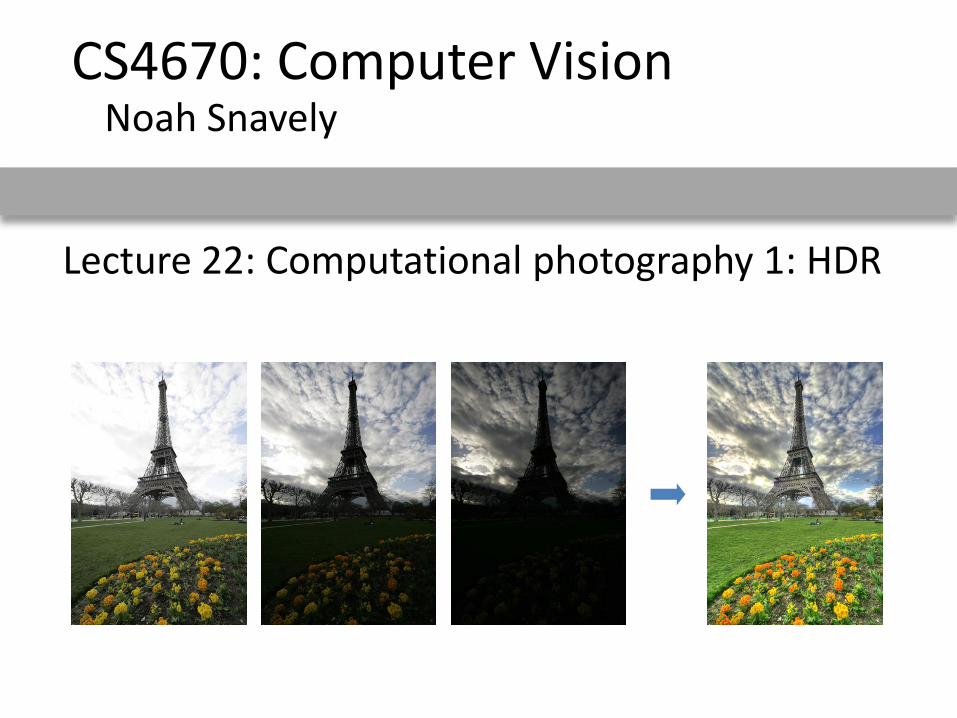
Lecture 22: Computational photography 1: HDR

CS4670: Computer VisionNoah Snavely

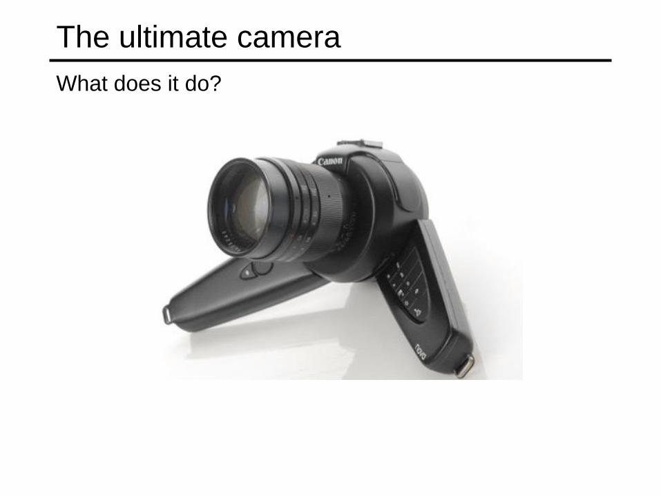
The ultimate camera

What does it do?

The ultimate camera

Infinite resolution

Infinite zoom control

Desired object(s) are in focus

No noise

No motion blur

Infinite dynamic range (can see dark and bright things)

...

Creating the ultimate camera

The ―analog‖ camera has changed very little in >100 yrs

• we’re unlikely to get there following this path

More promising is to combine ―analog‖ optics with

computational techniques

• ―Computational cameras‖ or ―Computational photography‖

This lecture will survey techniques for producing higher

quality images by combining optics and computation

Common themes:

• take multiple photos

• modify the camera

Noise reduction

Take several images and

average them

Why does this work?

Basic statistics:

• variance of the mean

decreases with n:

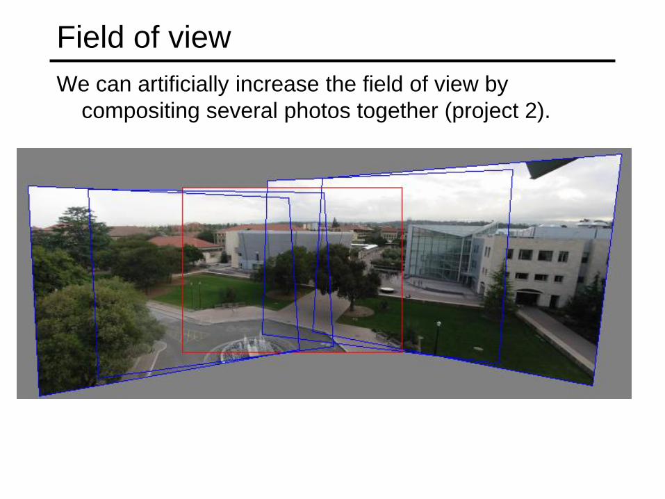
Field of view

We can artificially increase the field of view by

compositing several photos together (project 2).

Improving resolution: Gigapixel images

A few other notable examples:

• Obama inauguration (gigapan.org)

• HDView (Microsoft Research)

Max Lyons, 2003

fused 196 telephoto shots

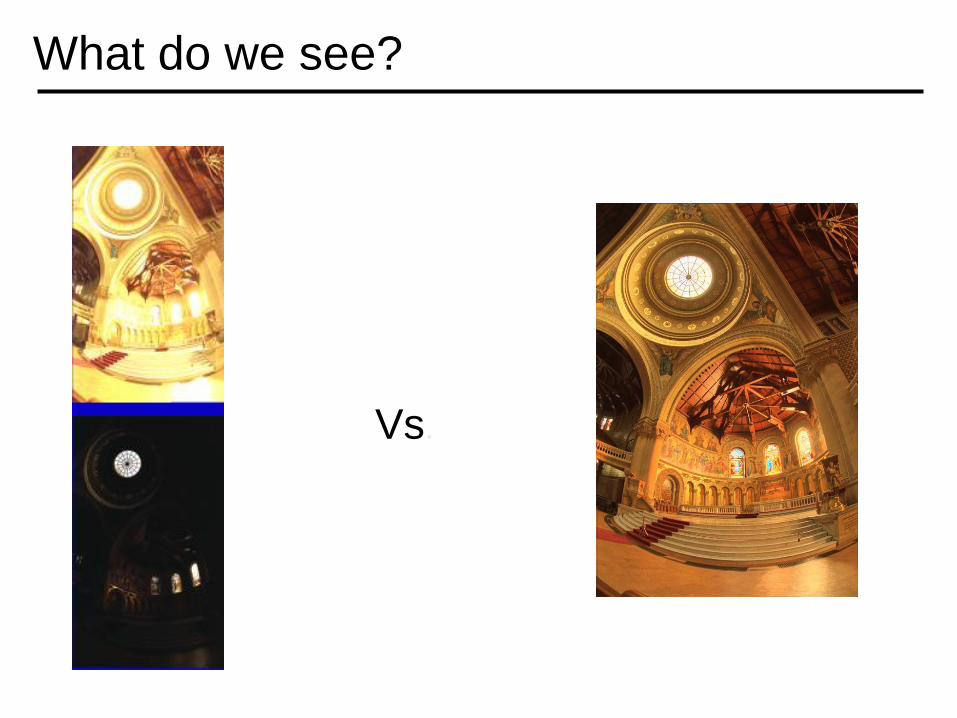
What do we see?

Vs.

Problem: Dynamic Range

1500

1

25,000

400,000

2,000,000,000

The real world is

high dynamic range.

Long Exposure

10-6 106

10-6 106

Real world

Picture

0 to 255

High dynamic range

Short Exposure

10-6 106

10-6 106

Real world

Picture

High dynamic range

0 to 255

pixel (312, 284) = 42

Image

42 photons?

Dynamic Range

Typical cameras have limited dynamic range

HDR images — merge multiple inputs

Scene Radiance

Pixel count

HDR images — merged

Radiance

Pixel count

Camera is not a photometer!

Limited dynamic range

• 8 bits captures only 2 orders of magnitude of light intensity

• We can see ~10 orders of magnitude of light intensity

Unknown, nonlinear response

• pixel intensity amount of light (# photons, or ―radiance‖)

Solution:

• Recover response curve from multiple exposures, then

reconstruct the radiance map

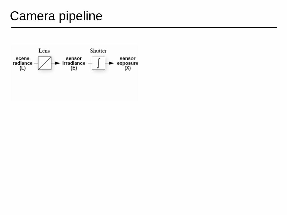
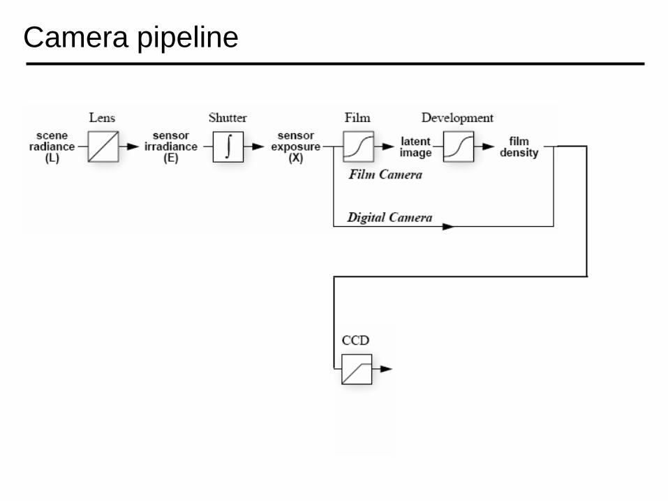
Camera pipeline

Camera pipeline

Camera pipeline

Camera pipeline

Camera pipeline

Camera pipeline

8 bits

)( tEfZ

log Exposure = log (Radiance * t)

Imaging system response function

Pixel

value

0

255

(CCD photon count)

Real-world response functions

In general, the response function is not provided

by camera makers who consider it part of their

proprietary product differentiation. In addition,

they are beyond the standard gamma curves.

Camera is not a photometer

• Limited dynamic range

Perhaps use multiple exposures?

• Unknown, nonlinear response

Not possible to convert pixel values to radiance

• Solution:

– Recover response curve from multiple exposures,

then reconstruct the radiance map

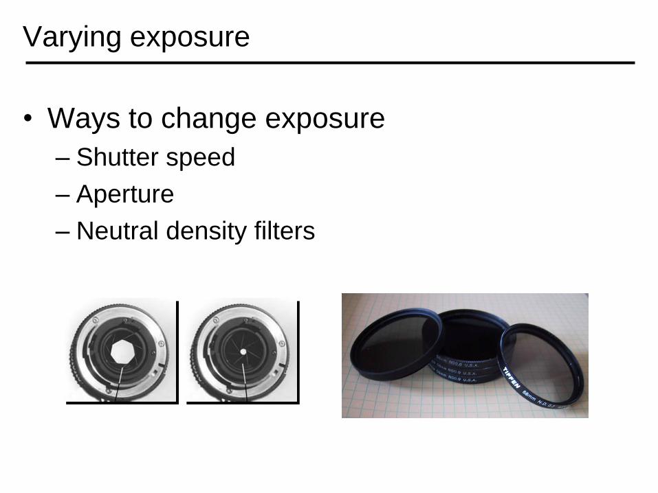
Varying exposure

• Ways to change exposure

– Shutter speed

– Aperture

– Neutral density filters

Shutter speed

• Note: shutter times usually obey a power series –each ―stop‖ is a factor of 2

• ¼, 1/8, 1/15, 1/30, 1/60, 1/125, 1/250, 1/500, 1/1000 sec

Usually really is:

¼, 1/8, 1/16, 1/32, 1/64, 1/128, 1/256, 1/512, 1/1024 sec

HDRI capturing from multiple exposures

• We want to obtain the response curve

•

3

•

1 •

2

t =

1/4 sec

•

3

•

1 •

2

t =

1 sec

•

3

• 1

• 2

t =

1/8 sec

•

3

•

1 •

2

t =

2 sec

Image series

•

3

•

1 •

2

t =

1/2 sec

HDRI capturing from multiple exposures

)( jiij tEfZ

jiij tEZf )(1

1ln where,lnln)( fgtEZg jiij

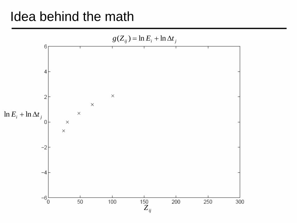
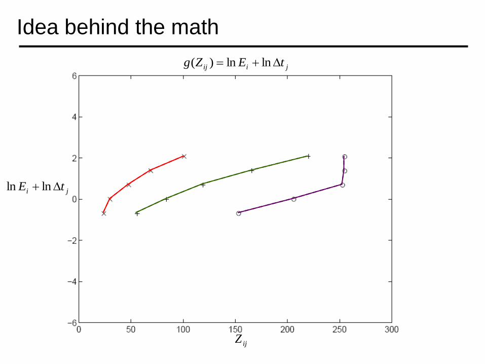
Idea behind the math

jiij tEZg lnln)(

ijZ

ji tE lnln

Idea behind the math

jiij tEZg lnln)(

ijZ

ji tE lnln

Idea behind the math

jiij tEZg lnln)(

ijZ

ji tE lnln

Math for recovering response curve

Recovering response curve

• The solution can be only up to a scale, add a

constraint

• Add a hat weighting function

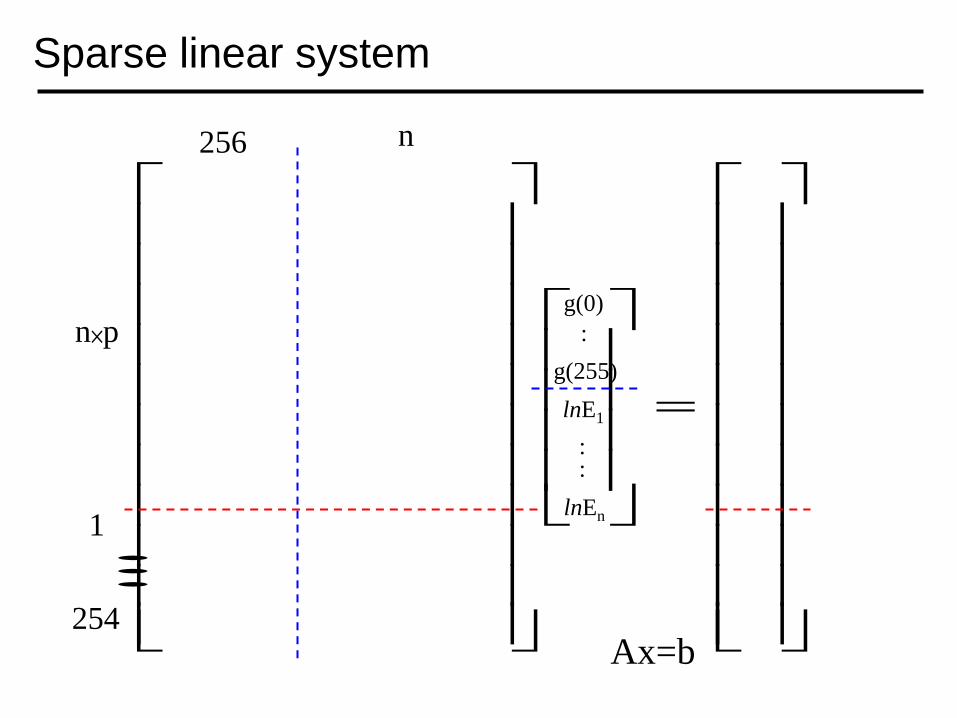
Sparse linear system

Ax=b

256 n

n×p

1

254

g(0)

g(255)

lnE1

lnEn

:

::

Matlab code

Matlab code

function [g,lE]=gsolve(Z,B,l,w)

n = 256;A = zeros(size(Z,1)*size(Z,2)+n+1,n+size(Z,1));b = zeros(size(A,1),1);

k = 1; %% Include the data-fitting equationsfor i=1:size(Z,1)

for j=1:size(Z,2)wij = w(Z(i,j)+1);A(k,Z(i,j)+1) = wij; A(k,n+i) = -wij; b(k,1) = wij * B(i,j);k=k+1;

endend

A(k,129) = 1; %% Fix the curve by setting its middle value to 0k=k+1;

for i=1:n-2 %% Include the smoothness equationsA(k,i)=l*w(i+1); A(k,i+1)=-2*l*w(i+1); A(k,i+2)=l*w(i+1);k=k+1;

end

x = A\b; %% Solve the system using SVD

g = x(1:n);lE = x(n+1:size(x,1));

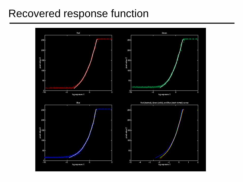
Recovered response function

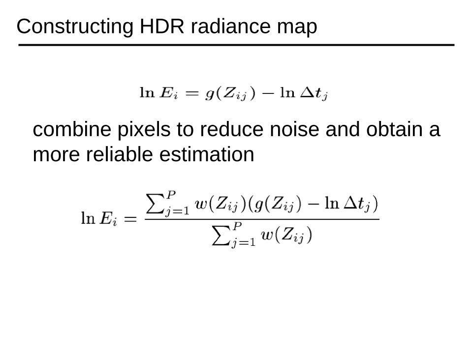
Constructing HDR radiance map

combine pixels to reduce noise and obtain a

more reliable estimation

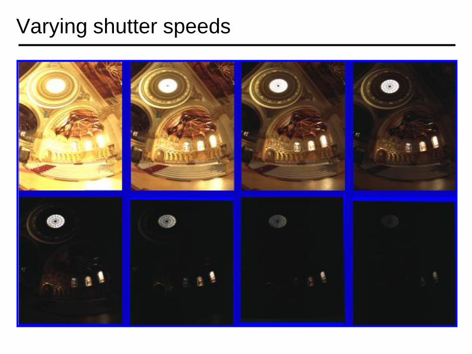
Varying shutter speeds

Reconstructed radiance map

What is this for?

• Human perception

• Vision/graphics applications

Assorted pixel (Single Exposure HDR)

Assorted pixel

Assorted pixel

detectorelement

attenuatorelement

It

Tt+1

controller

light

Pixel with Adaptive Exposure Control

Tone Mapping

10-6 106

10-6 106

Real World

Ray Traced

World (Radiance)

Display/

Printer

0 to 255

High dynamic range

• How can we do this?Linear scaling?, thresholding? Suggestions?

The

Radiance

Map

Linearly scaled to

display device

Simple Global Operator

• Compression curve needs to

– Bring everything within range

– Leave dark areas alone

• In other words

– Asymptote at 255

– Derivative of 1 at 0

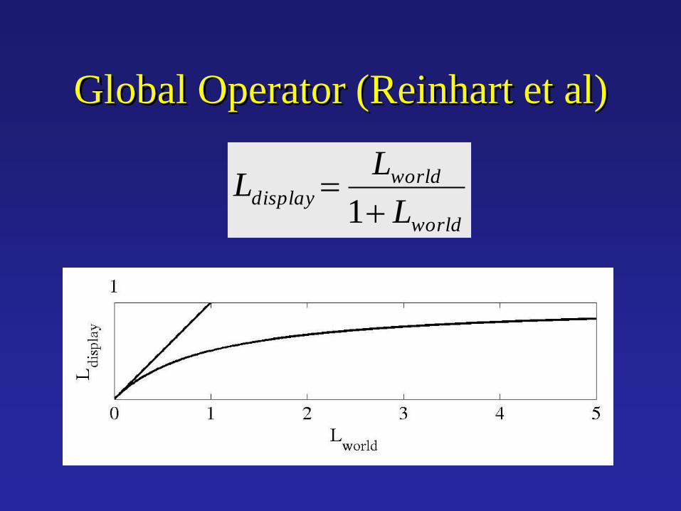
Global Operator (Reinhart et al)

world

worlddisplay

L

LL

1

Global Operator Results

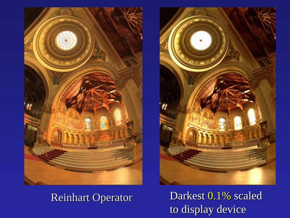
Darkest 0.1% scaled

to display deviceReinhart Operator

Questions?