CS340 Machine learningLecture 4

Learning theory

Some slides are borrowed from Sebastian Thrun and Stuart Russell

Announcement• What: Workshop on applying for NSERC

scholarships and for entry tograduate schoolWhen: Thursday, Sept 14, 12:30-14:00Where: DMP 110Who: All Computer Science undergraduates expecting to graduate withinthe next 12 months who are interested in applying to graduate school

PAC Learning: intuition• If we learn hypothesis h on the training data, how can be

sure this is close to the true target function f if we don't know what f is?

• Any hypothesis that we learn but which is seriously wrong will almost certainly be "found out" with high probability aftera small number of examples, because it will make an incorrect prediction.

• Thus any hypothesis that is consistent with a sufficiently large set of training examples is unlikely to be seriously wrong, i.e., it must be probably approximately correct.

• Learning theory is concerned with estimating the sample size needed to ensure good generalization performance.

PAC Learning• PAC = Probably approximately correct• Let f(x) be the true class, h(x) our guess, and π(x) a

distribution of examples. Define the error as

• Define h as approximately correct if error(h) < ε.• Goal: find sample size m s.t. for any distribution π

• If Ntrain >= m, then with probability 1-δ, the hypothesis will be approximately correct.

• Test examples must be drawn from same distribution as training examples.

• We assume there is no label noise.

Derivation of PAC bounds for finite H

• Partition H into Hε, an ε "ball" around ftrue, andHbad = H \ H ε

• What is the prob. that a "seriously wrong" hypothesis hb ∈ Hbad is consistent with m examples (so we are fooled)? We can use a union bound

The prob of finding such an hb is bounded by

Derivation of PAC bounds for finite H• We want to find m s.t.• This is called the sample complexity of H• We use to derive

• If |H| is larger, we need more training data to ensure we can choose the "right" hypothesis.

PAC Learnability• Statistical learning theory is concerned with sample

complexity.• Computational learning theory is additionally

concerned with computational (time) complexity.• A concept class C is PAC learnable, if it can be

learnt with probability δ and error ε in time polynomial in 1/δ, 1/ε, n, and size(c).

• Implies– Polynomial sample complexity– Polynomial computational time

H = any boolean function

• Consider all 222 = 16 possiblebinary functions on k=2 binary inputs

• If we observe (x1=0, x2=1, y=0), this removes h5, h6, h7, h8, h13, h14, h15, h16

• Each example halves the version space.• Still leaves exponentially many hypotheses!

H = any boolean function

Unbiased Learner: |H|=22k

))/1ln(2ln2(1 δε

+≥ km

• Needs exponentially large sample size to learn.• Essentially has to learn whole lookup table, since for anyunseen example, H contains as many consistent hypothesesthat predict 1 as 0.

Making learning tractable• To reduce the sample complexity, and allow

generalization from a finite sample, there are two approaches– Restrict the hypothesis space to simpler functions– Put a prior that encourages simpler functions

• We will consider the latter (Bayesian) approach later

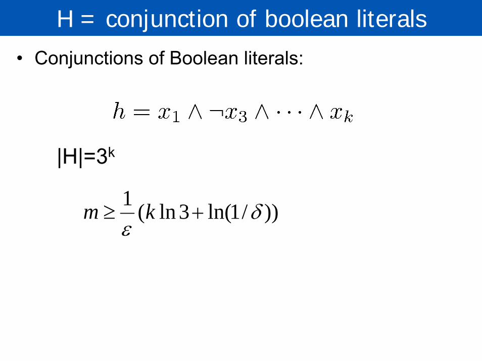
H = conjunction of boolean literals• Conjunctions of Boolean literals:

|H|=3k

))/1ln(3ln(1 δε

+≥ km

H = decision lists

H = decision lists

k-DL(n) restricts each test to contain at most k literals chosen from n attributesk-DL(n) includes the set of all decision trees of depth at most k

PAC bounds for rectangles• Let us consider an infinite hypothesis space, for which

|H| is not defined.• Let h be the most specific hypothesis, so errors occur in the

purple strips.

• Each strip is at most ε/4• Pr that we miss a strip 1‒ ε/4• Pr that N instances miss a strip (1 ‒ ε/4)N

• Pr that N instances miss 4 strips 4(1 ‒ ε/4)N

• 4(1 ‒ ε/4)N ≤ δ and (1 ‒ x)≤exp( ‒ x)• 4exp(‒ εN/4) ≤ δ and N ≥ (4/ε)log(4/δ)

VC Dimension• We can generalize the rectangle example using the

Vapnik-Chervonenkis dimension.• VC(H) is the maximum number of points that can

be shattered by H.• A set of instances S is shattered by H if for every

dichotomy (binary labeling) of S there is a consistent hypothesis in H.

• This is best explained by examples.

Shattering 3 points in R2 with circles

Is this set of points shattered by the hypothesis space H of all circles?

Shattering 3 points in R2 with circles

+

+ -

+

- +

-

+ +

+

+ +

-

- -

-

+ -

-

- +

+

- -

Every possible labeling can be covered by a circle, so we can shatter 3 points.

Is this set of points shattered by circles?

Is this set of points shattered by circles?

No, we cannot shatter any set of 4 points.

How About This One?

How About This One?

We cannot shatter this set of 3 points,but we can find some set of 3 points which we can shatter

VCD(Circles)=3

• VC(H) = 3, since 3 points can beshattered but not 4

VCD(Axes-Parallel Rectangles) = 4

Can shatter at most 4 points in R2 with a rectangle

Linear decision surface in 2D

VC(H) = 3, so xor problem is notlinearly separable

Linear decision surface in n-d

VC(H) = n+1

Is there an H with VC(H)=∞ ?

Yes! The space of all convex polygons

PAC-Learning with VC-dim.

• Theorem: After seeing

random training examples the learner will with probability 1-δ generate a hypothesis with error at most ε.

))/13(log)(8)/2(log4(122 εδ

εHVCm +≥

Criticisms of PAC learning• The bounds on the generalization error are very

loose, because– they are distribution free/ worst case bounds, and do not

depend on the actual observed data– they make various approximations

• Consequently the bounds are not very useful in practice.