CS 8751 ML & KDD Evaluating Hypotheses 1

Evaluating Hypotheses • Sample error, true error

• Confidence intervals for observed hypothesis error

• Estimators

• Binomial distribution, Normal distribution,

Central Limit Theorem

• Paired t-tests

• Comparing Learning Methods

CS 8751 ML & KDD Evaluating Hypotheses 2

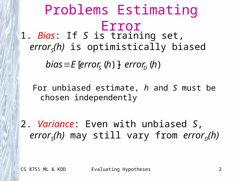
Problems Estimating Error1. Bias: If S is training set, errorS(h) is optimistically

biased

For unbiased estimate, h and S must be chosen independently

2. Variance: Even with unbiased S, errorS(h) may still vary from errorD(h)

)()]([ herrorherrorEbias DS

CS 8751 ML & KDD Evaluating Hypotheses 3

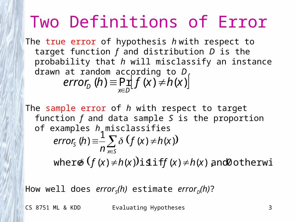
Two Definitions of ErrorThe true error of hypothesis h with respect to target function f

and distribution D is the probability that h will misclassify an instance drawn at random according to D.

The sample error of h with respect to target function f and data sample S is the proportion of examples h misclassifies

How well does errorS(h) estimate errorD(h)?

)()(Pr)( xhxfherrorDx

D

otherwise 0 and ),()( if 1 is )()( where

)()( 1

)(

xhxfxhxf

xhxfn

herrorSx

S

CS 8751 ML & KDD Evaluating Hypotheses 4

ExampleHypothesis h misclassifies 12 of 40 examples in S.

What is errorD(h)?

30.40

12)( herrorS

CS 8751 ML & KDD Evaluating Hypotheses 5

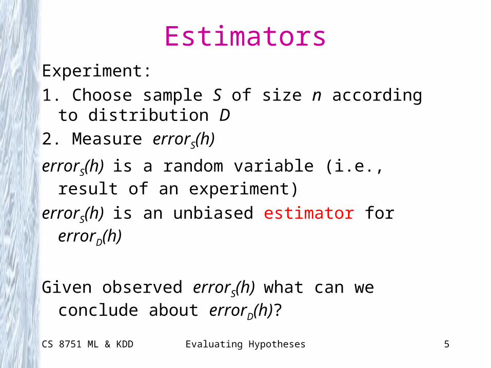
EstimatorsExperiment:

1. Choose sample S of size n according to distribution D

2. Measure errorS(h)

errorS(h) is a random variable (i.e., result of an experiment)

errorS(h) is an unbiased estimator for errorD(h)

Given observed errorS(h) what can we conclude about errorD(h)?

CS 8751 ML & KDD Evaluating Hypotheses 6

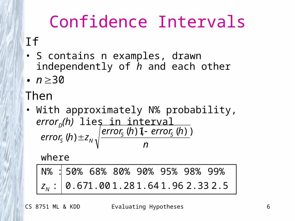
Confidence IntervalsIf• S contains n examples, drawn independently of h and each

other

• Then• With approximately N% probability, errorD(h) lies in

interval

30n

2.53 2.33 1.96 1.64 1.28 1.00 0.67 :

99% 98% 95% 90% 80% 68% 50% :N%

where

))(1)(()(

N

SSNS

z

n

herrorherrorzherror

CS 8751 ML & KDD Evaluating Hypotheses 7

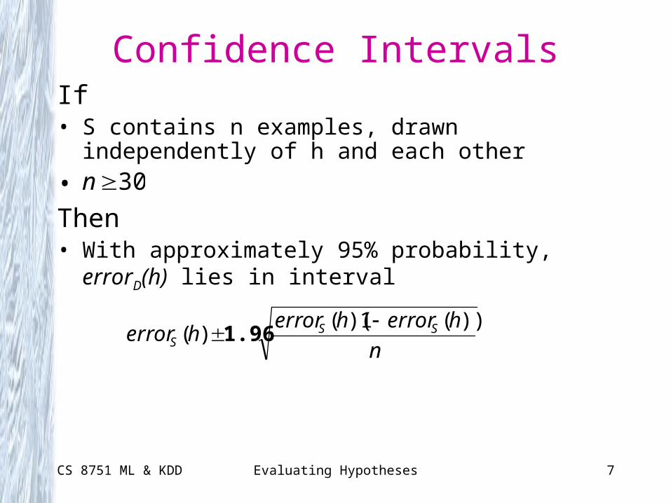
Confidence IntervalsIf• S contains n examples, drawn independently of h and each

other

• Then• With approximately 95% probability, errorD(h) lies in

interval

30n

n

herrorherrorherror SS

S

))(1)(()(

1.96

CS 8751 ML & KDD Evaluating Hypotheses 8

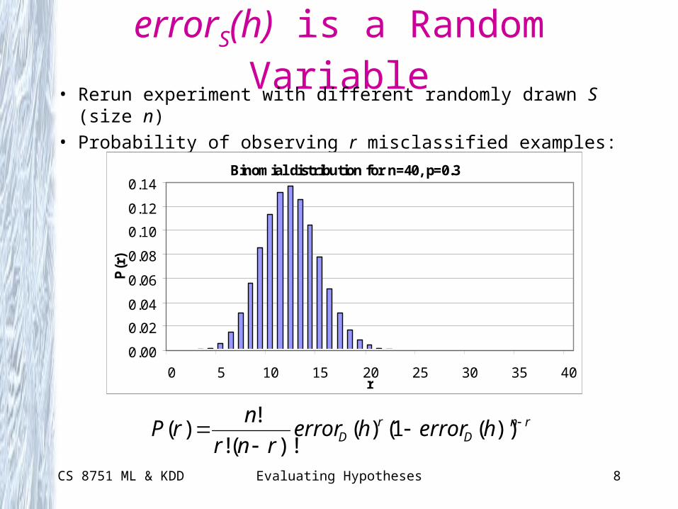
errorS(h) is a Random Variable• Rerun experiment with different randomly drawn S (size n)

• Probability of observing r misclassified examples:

Binomial distribution for n=40, p=0.3

0.00

0.02

0.04

0.06

0.08

0.10

0.12

0.14

0 5 10 15 20 25 30 35 40r

P(r)

rnD

rD herrorherror

rnr

nrP

))(1()(

)!(!

!)(

CS 8751 ML & KDD Evaluating Hypotheses 9

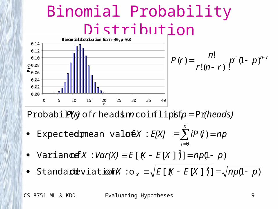
Binomial Probability DistributionBinomial distribution for n=40, p=0.3

0.00

0.02

0.04

0.06

0.08

0.10

0.12

0.14

0 5 10 15 20 25 30 35 40r

P(r)

rnr pprnr

nrP

)1(

)!(!

!)(

)1(]])[[(σ : ofdeviation Standard

)1(]])[[( : of Variance

)( : of mean valueor Expected,

Pr if flips,coin in heads of Probabilty

2

2

0

pnpXEXEX

pnpXEXEVar(X)X

npiiPE[X] X

(heads)pnrP(r)

X

n

i

CS 8751 ML & KDD Evaluating Hypotheses 10

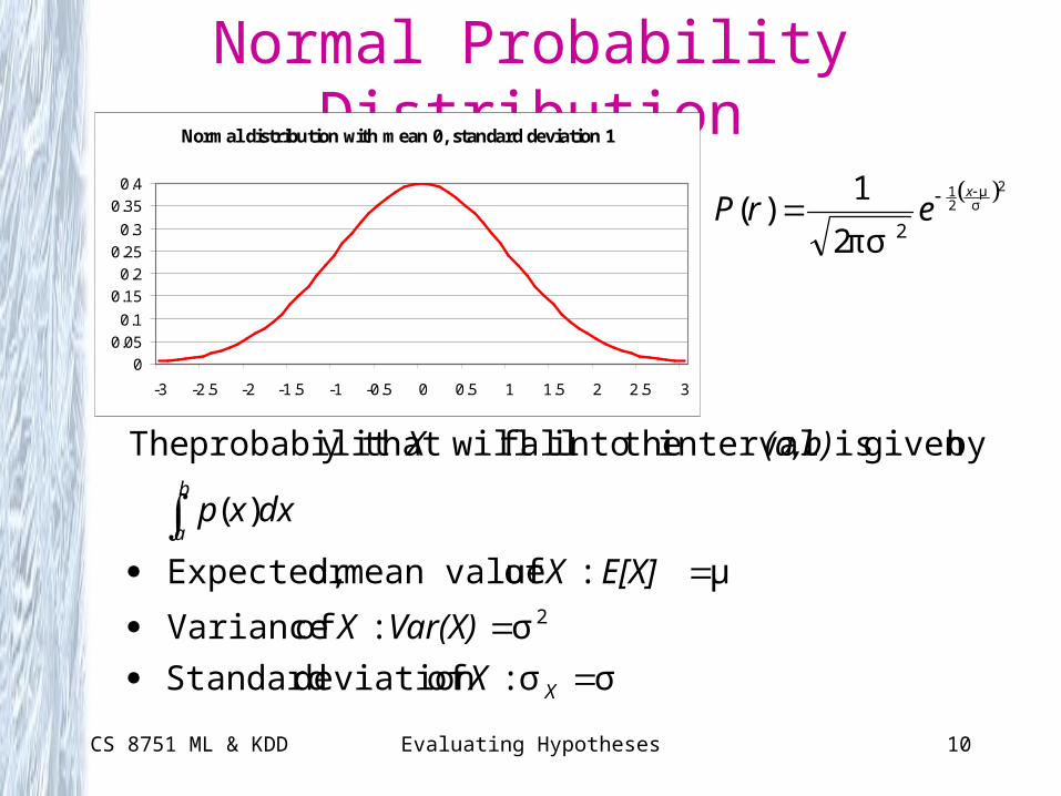
Normal Probability DistributionNormal distribution with mean 0, standard deviation 1

0

0.05

0.1

0.15

0.2

0.25

0.3

0.35

0.4

-3 -2.5 -2 -1.5 -1 -0.5 0 0.5 1 1.5 2 2.5 3

2σμ

21

2πσ2

1)(

x

erP

σσ : ofdeviation Standard

: of Variance

μ : of mean valueor Expected,

)(

bygiven is interval theinto fall willy that probabilit The

2

X

b

a

X

Var(X)X

E[X] X

dxxp

(a,b)X

σ

CS 8751 ML & KDD Evaluating Hypotheses 11

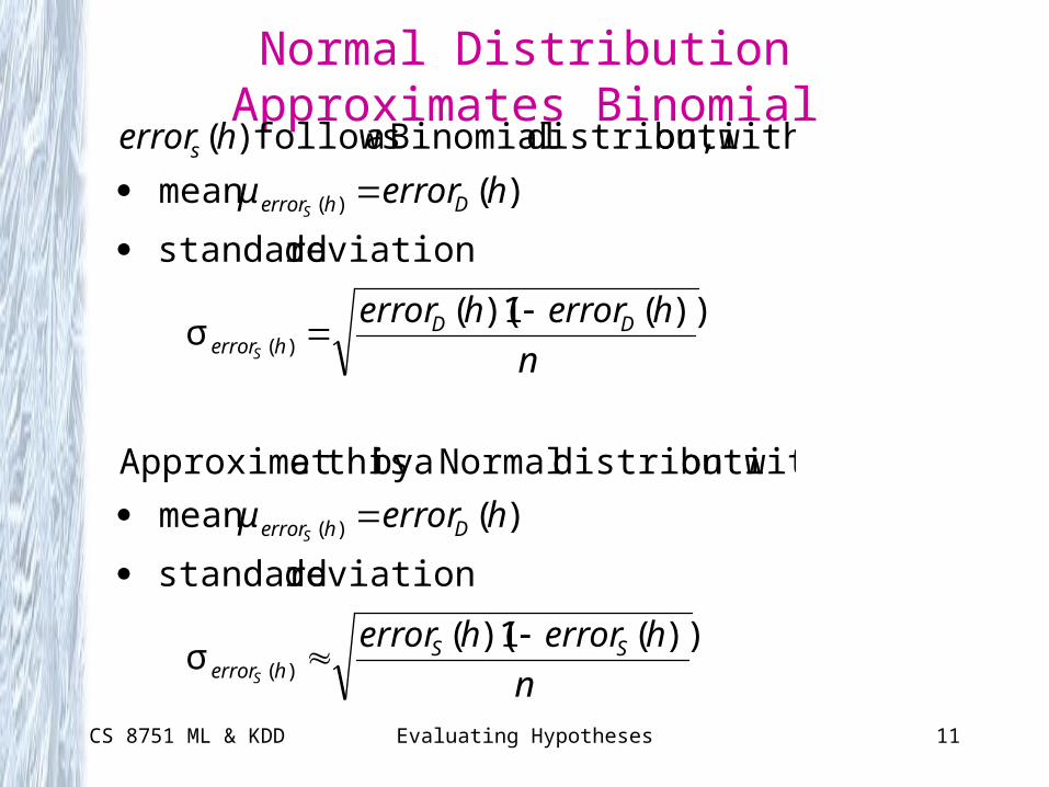
Normal Distribution Approximates Binomial

n

herrorherror

herrorμ

n

herrorherror

herrorμ

herror

SSherror

Dherror

DDherror

Dherror

s

S

S

S

S

))(1)((σ

deviation standard

)(mean

on withdistributi Normal aby thiseApproximat

))(1)((σ

deviation standard

)(mean

withon,distributi Binomial a follows )(

)(

)(

)(

)(

CS 8751 ML & KDD Evaluating Hypotheses 12

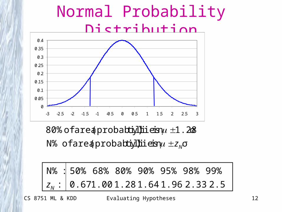
Normal Probability Distribution

0

0.05

0.1

0.15

0.2

0.25

0.3

0.35

0.4

-3 -2.5 -2 -1.5 -1 -0.5 0 0.5 1 1.5 2 2.5 3

2.53 2.33 1.96 1.64 1.28 1.00 0.67 :

99% 98% 95% 90% 80% 68% 50% :N%

σ in lies ty)(probabili area of N%

σ1.28 in lies ty)(probabili area of 80%

N

N

z

z

CS 8751 ML & KDD Evaluating Hypotheses 13

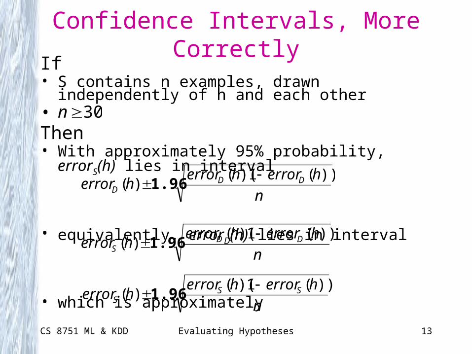
Confidence Intervals, More CorrectlyIf• S contains n examples, drawn independently of h and each

other• Then• With approximately 95% probability, errorS(h) lies in

interval

• equivalently, errorD(h) lies in interval

• which is approximately

30n

n

herrorherrorherror DD

D

))(1)(()(

1.96

n

herrorherrorherror DD

S

))(1)(()(

1.96

n

herrorherrorherror SS

S

))(1)(()(

1.96

CS 8751 ML & KDD Evaluating Hypotheses 14

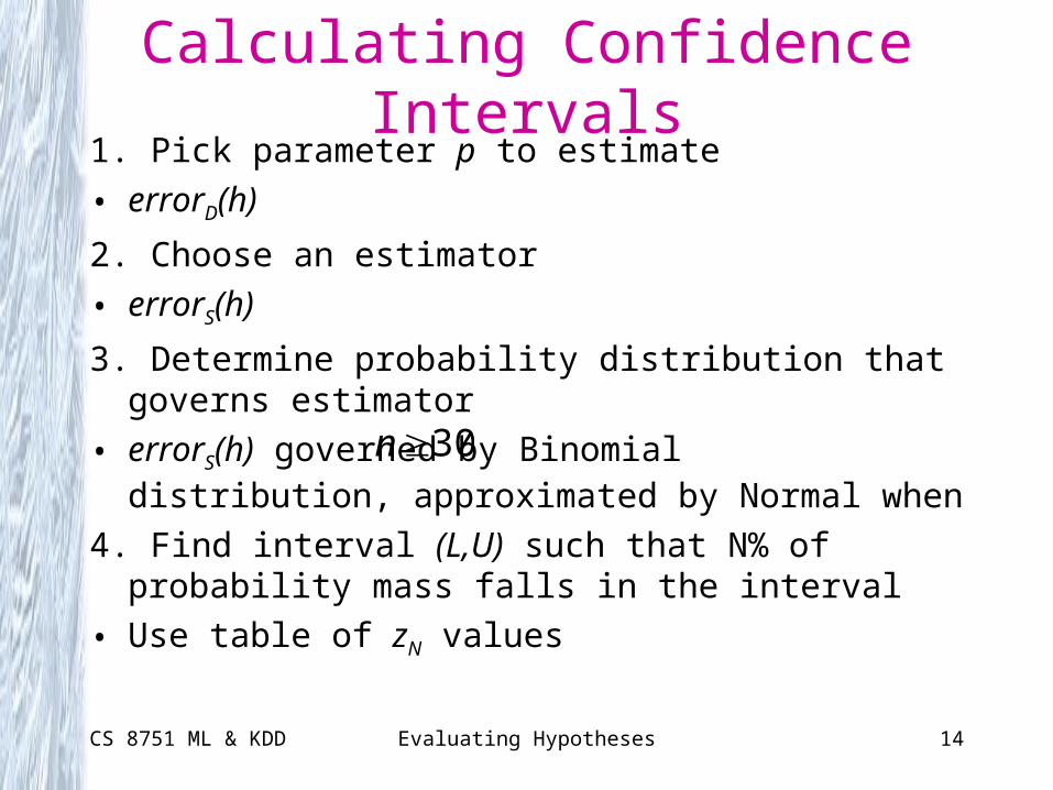
Calculating Confidence Intervals1. Pick parameter p to estimate

• errorD(h)

2. Choose an estimator

• errorS(h)

3. Determine probability distribution that governs estimator

• errorS(h) governed by Binomial distribution, approximated by Normal when

4. Find interval (L,U) such that N% of probability mass falls in the interval

• Use table of zN values

30n

CS 8751 ML & KDD Evaluating Hypotheses 15

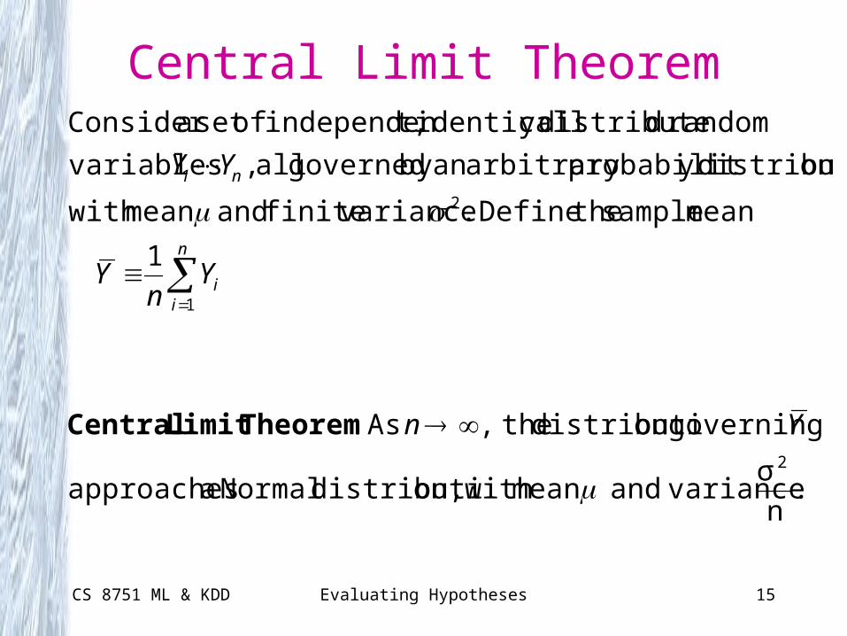
Central Limit Theorem

.n

σ varianceand mean with on,distributi Normal a approaches

governingon distributi the, As .

1

mean sample theDefine . variancefinite and mean with

ondistributiy probabilitarbitrary an by governed all , variables

random ddistributey identicall t,independen ofset aConsider

2

1

2

Yn

Yn

Yn

ii

TheoremLimit Central

n1 YY

CS 8751 ML & KDD Evaluating Hypotheses 16

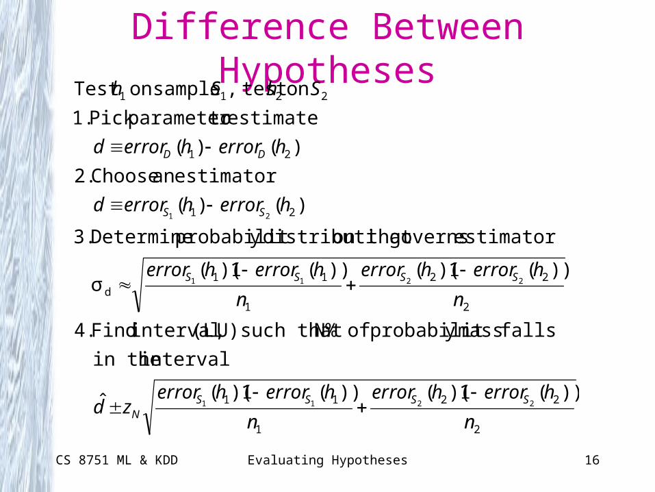
Difference Between Hypotheses

2

22

1

11

2

22

1

11d

21

21

2211

))(1)(())(1)((ˆ

interval in the

falls massy probabilit of N%such that U)(L, interval Find 4.

))(1)(())(1)((σ

estimator governson that distributiy probabilit Determine 3.

)()(

estimatoran Choose 2.

)()(

estimate toparameter Pick 1.

on test , sampleon Test

2211

2211

21

n

herrorherror

n

herrorherrorzd

n

herrorherror

n

herrorherror

herrorherrord

herrorherrord

ShSh

SSSSN

SSSS

SS

DD

CS 8751 ML & KDD Evaluating Hypotheses 17

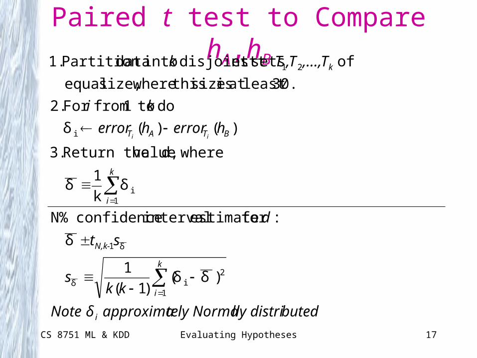
Paired t test to Compare hA,hB

butedlly distritely Norma approximaNote δ

kks

st

d

herrorherror

ki

,...,T,TTk

i

k

i

N,k-

k

i

BTAT

k

ii

1

2iδ

δ1

1i

i

21

)δδ()1(

1

δ

:for estimate interval confidence N%

δk

1δ

whered, valueReturn the 3.

)()(δ

do to1 from For 2.

30.least at is size this wheresize, equal

of setsest disjoint t into dataPartition 1.

CS 8751 ML & KDD Evaluating Hypotheses 18

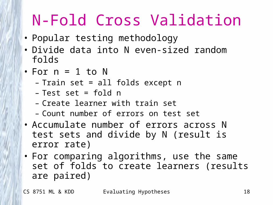
N-Fold Cross Validation• Popular testing methodology• Divide data into N even-sized random folds• For n = 1 to N

– Train set = all folds except n– Test set = fold n– Create learner with train set– Count number of errors on test set

• Accumulate number of errors across N test sets and divide by N (result is error rate)

• For comparing algorithms, use the same set of folds to create learners (results are paired)

CS 8751 ML & KDD Evaluating Hypotheses 19

N-Fold Cross Validation• Advantages/disadvantages

– Estimate of error within a single data set

– Every point used once as a test point

– At the extreme (when N = size of data set), called leave-one-out testing

– Results affected by random choices of folds (sometimes answered by choosing multiple random folds – Dietterich in a paper expressed significant reservations)

CS 8751 ML & KDD Evaluating Hypotheses 20

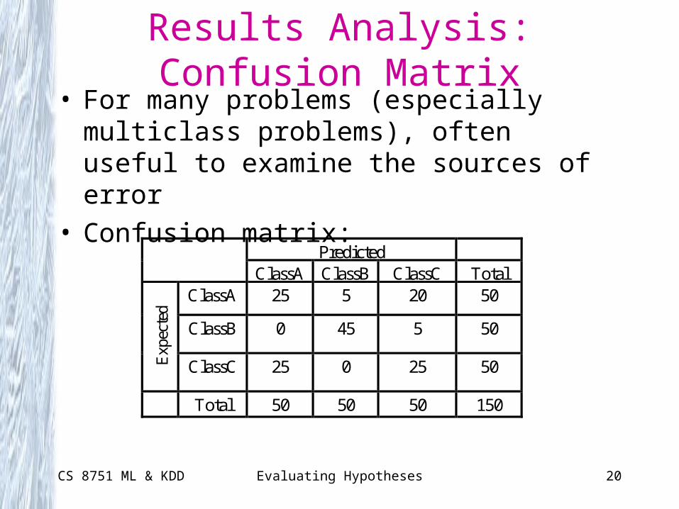
Results Analysis: Confusion Matrix• For many problems (especially multiclass

problems), often useful to examine the sources of error

• Confusion matrix:

Predicted ClassA ClassB ClassC Total

ClassA 25 5 20 50

ClassB 0 45 5 50

Exp

ecte

d

ClassC 25 0 25 50

Total 50 50 50 150

CS 8751 ML & KDD Evaluating Hypotheses 21

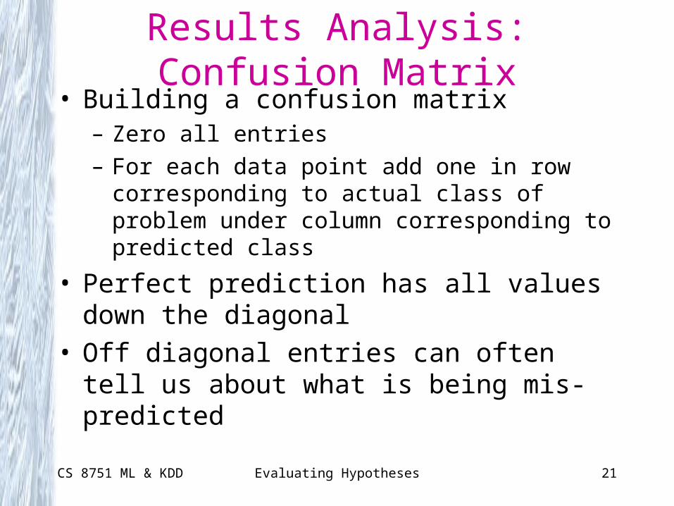
Results Analysis: Confusion Matrix• Building a confusion matrix

– Zero all entries

– For each data point add one in row corresponding to actual class of problem under column corresponding to predicted class

• Perfect prediction has all values down the diagonal

• Off diagonal entries can often tell us about what is being mis-predicted

CS 8751 ML & KDD Evaluating Hypotheses 22

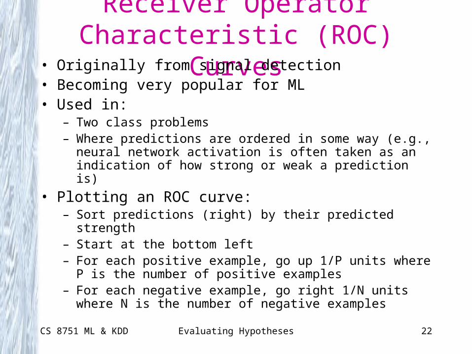
Receiver Operator Characteristic (ROC) Curves

• Originally from signal detection• Becoming very popular for ML• Used in:

– Two class problems– Where predictions are ordered in some way (e.g., neural network

activation is often taken as an indication of how strong or weak a prediction is)

• Plotting an ROC curve:– Sort predictions (right) by their predicted strength– Start at the bottom left– For each positive example, go up 1/P units where P is the number

of positive examples– For each negative example, go right 1/N units where N is the

number of negative examples

CS 8751 ML & KDD Evaluating Hypotheses 23

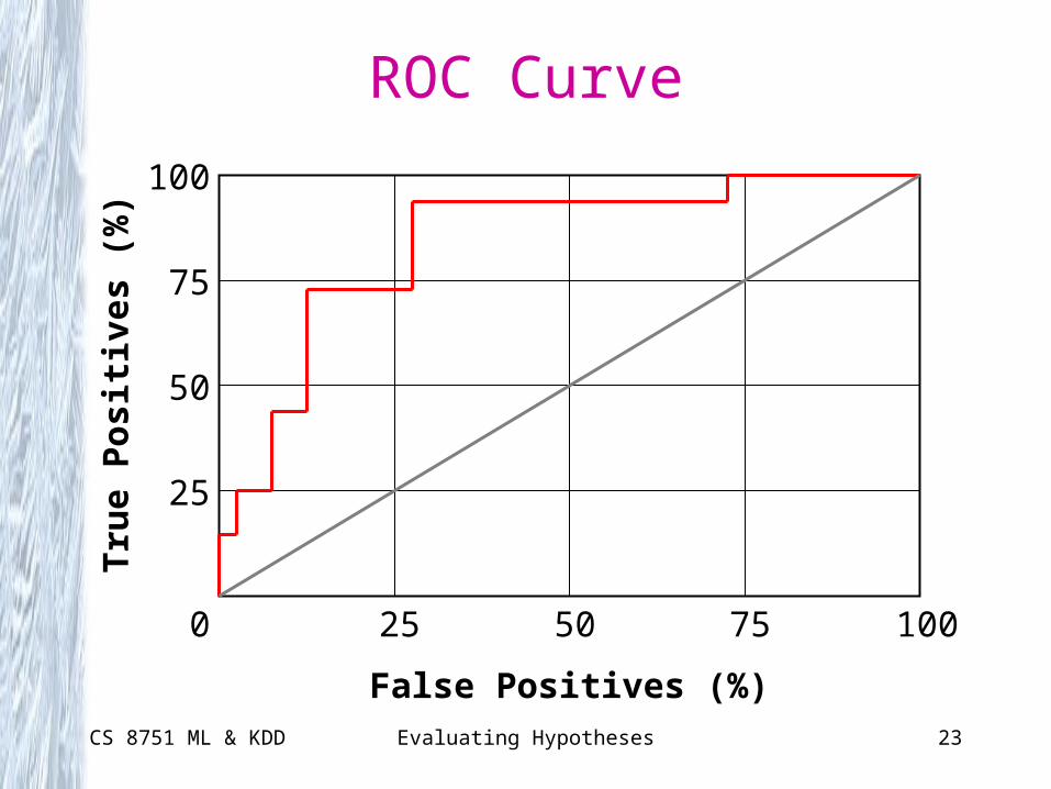
ROC Curve

25 50 75 1000

25

50

75

100

False Positives (%)

True Positives (%)

CS 8751 ML & KDD Evaluating Hypotheses 24

ROC Properties• Can visualize the tradeoff between coverage and accuracy

(as we lower the threshold for prediction how many more true positives will we get in exchange for more false positives)

• Gives a better feel when comparing algorithms– Algorithms may do well in different portions of the curve

• A perfect curve would start in the bottom left, go to the top left, then over to the top right– A random prediction curve would be a line from the bottom left to

the top right

• When comparing curves:– Can look to see if one curve dominates the other (is always better)– Can compare the area under the curve (very popular – some

people even do t-tests on these numbers)