cs 5600 computer systems lecture 6: process scheduling

CS 5600Computer Systems

Lecture 6: Process Scheduling

2

• Scheduling Basics• Simple Schedulers• Priority Schedulers• Fair Share Schedulers• Multi-CPU Scheduling• Case Study: The Linux Kernel

3

Setting the Stage

• Suppose we have:– A computer with N CPUs– P process/threads that are ready to run

• Questions we need to address:– In what order should the processes be run?– On what CPU should each process run?

4

Factors Influencing Scheduling• Characteristics of the processes– Are they I/O bound or CPU bound?– Do we have metadata about the processes?

• Example: deadlines

– Is their behavior predictable?• Characteristics of the machine– How many CPUs?– Can we preempt processes?– How is memory shared by the CPUs?

• Characteristics of the user– Are the processes interactive (e.g. desktop apps)…– Or are the processes background jobs?

5

Basic Scheduler Architecture• Scheduler selects from the ready processes, and

assigns them to a CPU– System may have >1 CPU– Various different approaches for selecting processes

• Scheduling decisions are made when a process:1. Switches from running to waiting2. Terminates3. Switches from running to ready4. Switches from waiting to ready

• Scheduler may have access to additional information– Process deadlines, data in shared memory, etc.

No preemption

Preemption

6

Dispatch Latency• The dispatcher gives control of the CPU to the

process selected by the scheduler– Switches context– Switching to/from kernel mode/user mode– Saving the old EIP, loading the new EIP

• Warning: dispatching incurs a cost– Context switching and mode switch are expensive– Adds latency to processing times

• It is advantageous to minimize process switching

7

A Note on Processes & Threads

• Let’s assume that processes and threads are equivalent for scheduling purposes– Kernel supports threads• System-contention scope (SCS)

– Each process has >=1 thread• If kernel does not support threads– Each process handles it’s own thread scheduling– Process contention scope (PCS)

8

Basic Process Behavior• Processes alternate

between doing work and waiting– Work CPU Burst

• Process behavior varies– I/O bound– CPU bound

• Expected CPU burst distribution is important for scheduler design– Do you expect more CPU

or I/O bound processes?

Process 1 Process 2

Execute Code

Execute Code

Execute Code

Execute Code

Execute Code

Waiting on I/O

Waiting for mutex

sleep(1)

CPU Burst

Wait

Waiting on I/O

Waiting on I/O

9

Scheduling Optimization Criteria• Max CPU utilization – keep the CPU as busy as possible• Max throughput – # of processes that finish over time– Min turnaround time – amount of time to finish a process– Min waiting time – amount of time a ready process has

been waiting to execute• Min response time – amount time between submitting

a request and receiving a response– E.g. time between clicking a button and seeing a response

• Fairness – all processes receive min/max fair CPU resources

• No scheduler can meet all these criteria• Which criteria are most important depend on types of processes

and expectations of the system• E.g. response time is key on the desktop• Throughput is more important for MapReduce

10


11

First Come, First Serve (FCFS)• Simple scheduler– Processes stored in a FIFO queue– Served in order of arrival

Process Burst Time

Arrival Time

P1 24 0.000

P2 3 0.001

P3 3 0.002

P1 P2 P3Time: 0 24 27 30

• Turnaround time = completion time - arrival time – P1 = 24; P2 = 27; P3 = 30– Average turnaround time: (0 + 24 + 27) / 3 = 27

12

The Convoy Effect• FCFS scheduler, but the arrival order has changed

P1P2 P3Time: 0 3 6 30

• Turnaround time: P1 = 30; P2 =3; P3 = 6– Average turnaround time: (30 + 3 + 6) / 3 = 13– Much better than the previous arrival order!

• Convoy effect (a.k.a. head-of-line blocking)– Long process can impede short processes– E.g.: CPU bound process followed by I/O bound process

Process Burst Time

Arrival Time

P1 24 0.002

P2 3 0.000

P3 3 0.001

13

Shortest Job First (SJF)• Schedule processes based on the length of

their next CPU burst time– Shortest processes go first

Process Burst Time

Arrival Time

P1 6 0

P2 8 0

P3 7 0

P4 3 0

P3P4 P1Time: 0 3 9 16

P224

• Average turnaround time: (3 + 16 + 9 + 0) / 4 = 7• SJF is optimal: guarantees minimum average wait

time

14

Predicting Next CPU Burst Length• Problem: future CPU burst times may be unknown• Solution: estimate the next burst time based on

previous burst lengths– Assumes process behavior is not highly variable– Use exponential averaging• tn – measured length of the nth CPU burst

• τn+1 – predicted value for n+1th CPU burst• α – weight of current and previous measurements (0 ≤ α ≤ 1)• τn+1 = αtn + (1 – α) τn

– Typically, α = 0.5

15

0

2

4

6

8

10

12

14

6

4

6

4

13 13 13

10

8

6 6

5

9

11

12

Actual and Estimated CPU Burst Times

True CPU Burst Length Estimated Burst Length

Time

Burs

t Len

gth

16

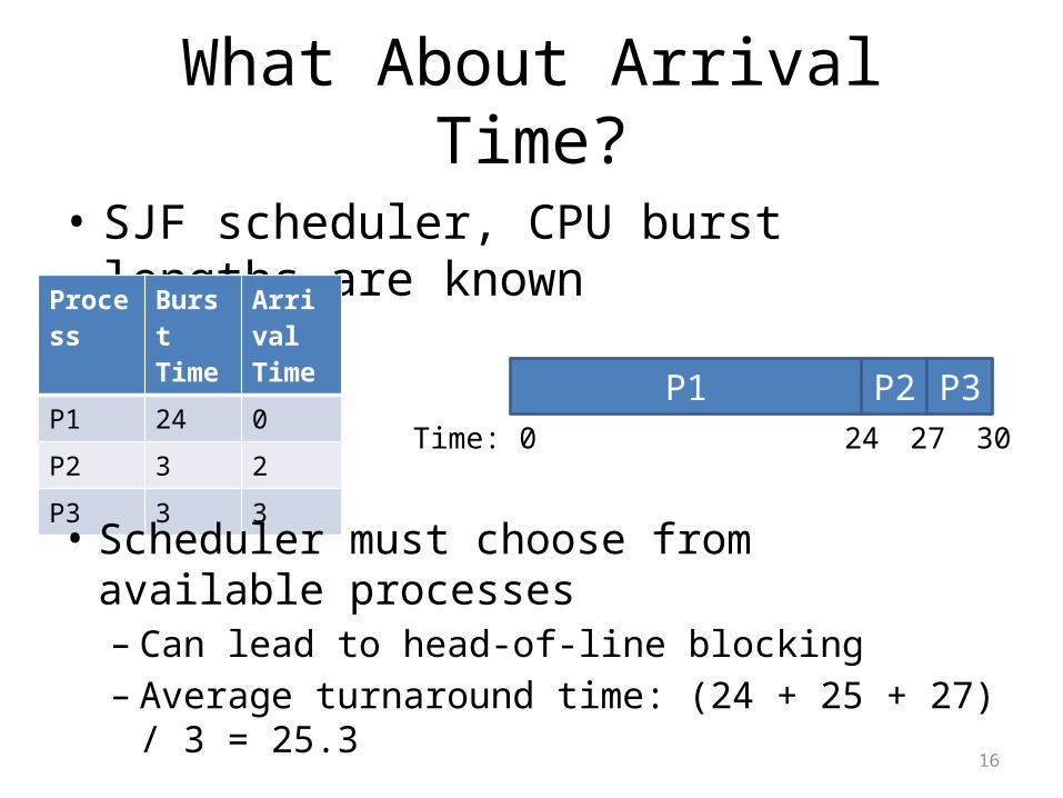
What About Arrival Time?

• SJF scheduler, CPU burst lengths are knownProcess Burst

TimeArrival Time

P1 24 0

P2 3 2

P3 3 3

P1 P2 P3Time: 0 24 27 30

• Scheduler must choose from available processes– Can lead to head-of-line blocking– Average turnaround time: (24 + 25 + 27) / 3 = 25.3

17

Shortest Time-To-Completion First (STCF)• Also known as Preemptive SJF (PSJF)– Processes with long bursts can be context

switched out in favor or short processes Process Burst

TimeArrival Time

P1 24 0

P2 3 2

P3 3 3

P1 P2 P3Time: 0 2 5 8

P130

• Turnaround time: P1 = 30; P2 = 3; P3 = 5– Average turnaround time: (30 + 3 + 5) / 3 = 12.7

• STCF is also optimal– Assuming you know future CPU burst times

18

Interactive Systems

• Imagine you are typing/clicking in a desktop app– You don’t care about turnaround time– What you care about is responsiveness• E.g. if you start typing but the app doesn’t show the text for

10 seconds, you’ll become frustrated

• Response time = first run time – arrival time

19

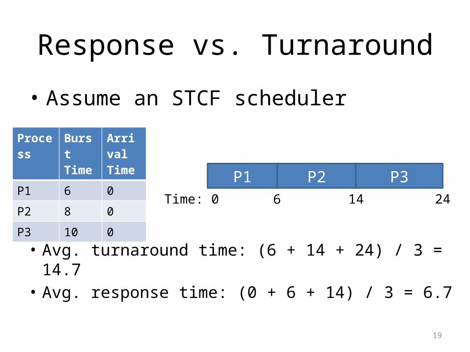
Response vs. Turnaround

• Assume an STCF scheduler

Process Burst Time

Arrival Time

P1 6 0

P2 8 0

P3 10 0

P1Time: 0 6 24

P2 P314

• Avg. turnaround time: (6 + 14 + 24) / 3 = 14.7• Avg. response time: (0 + 6 + 14) / 3 = 6.7

20

Round Robin (RR)

• Round robin (a.k.a time slicing) scheduler is designed to reduce response times– RR runs jobs for a time slice (a.k.a. scheduling

quantum)– Size of time slice is some multiple of the timer-

interrupt period

21

RR vs. STCFProcess Burst

TimeArrival Time

P1 6 0

P2 8 0

P3 10 0

P1Time: 0 6 24

P2 P314

• Avg. turnaround time: (6 + 14 + 24) / 3 = 14.7• Avg. response time: (0 + 6 + 14) / 3 = 6.7

P1

Time: 0 2

• 2 second time slices• Avg. turnaround time: (14 + 20 + 24) / 3 = 19.3• Avg. response time: (0 + 2 + 4) / 3 = 2

P2 P3 P1 P2 P3 P1 P2 P3 P2 P3

4 6 8 10 12 14 16 18 20 24

STCF

RR

22

TradeoffsRR

+ Excellent response times+ With N process and time slice of

Q…+ No process waits more than (N-

1)/Q time slices+ Achieves fairness

+ Each process receives 1/N CPU time- Worst possible turnaround times

- If Q is large FIFO behavior

STCF+ Achieves optimal, low

turnaround times- Bad response times- Inherently unfair

- Short jobs finish first

• Optimizing for turnaround or response time is a trade-off• Achieving both requires more sophisticated algorithms

23

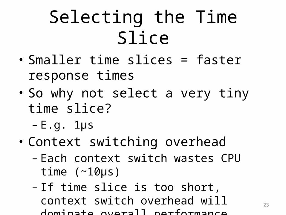
Selecting the Time Slice

• Smaller time slices = faster response times• So why not select a very tiny time slice?– E.g. 1µs

• Context switching overhead– Each context switch wastes CPU time (~10µs)– If time slice is too short, context switch overhead

will dominate overall performance• This results in another tradeoff– Typical time slices are between 1ms and 100ms

24

Incorporating I/O

• How do you incorporate I/O waits into the scheduler?– Treat time in-between I/O waits as CPU burst time

Process Total Time

Burst Time

Wait Time

Arrival Time

P1 22 5 5 0

P2 20 20 0 0

P1

Time: 0 5

P2

10 15 20 25 30 35 40

P1 P2 P1 P2 P1 P2

P1

CPU

Disk P1 P1 P1

P1

42

STCF Scheduler

25


26

Status Check

• Introduced two different types of schedulers– SJF/STCF: optimal turnaround time– RR: fast response time

• Open problems:– Ideally, we want fast response time and turnaround• E.g. a desktop computer can run interactive and CPU

bound processes at the same time

– SJF/STCF require knowledge about burst times• Both problems can be solved by using

prioritization

27

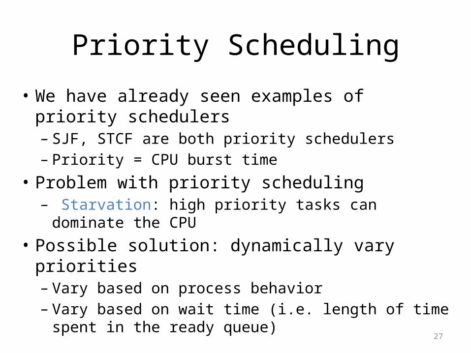
Priority Scheduling

• We have already seen examples of priority schedulers– SJF, STCF are both priority schedulers– Priority = CPU burst time

• Problem with priority scheduling– Starvation: high priority tasks can dominate the CPU

• Possible solution: dynamically vary priorities– Vary based on process behavior– Vary based on wait time (i.e. length of time spent in

the ready queue)

28

Simple Priority Scheduler

Process Burst Time Arrival Time Priority

P1 10 0 3

P2 2 0 1

P3 3 0 4

P4 2 0 5

P5 5 0 2

P2Time: 0 2 22

P5 P117

• Avg. turnaround time: (17 + 2 + 20 + 22 + 7) / 5 = 13.6• Avg. response time: (7 + 0 + 17 + 20 + 2) / 5 = 9.2

P3 P47 20

• Associate a priority with each process– Schedule high priority tasks first– Lower numbers = high priority– No preemption

• Cannot automatically balance response vs. turnaround time• Prone to starvation

29

Earliest Deadline First (EDF)• Each process has a deadline it must finish by• Priorities are assigned according to deadlines– Tighter deadlines are given higher priority

• EDF is optimal (assuming preemption)• But, it’s only useful if processes have known deadlines– Typically used in real-time OSes

Process Burst Time

Arrival Time

Deadline

P1 15 0 40

P2 3 4 10

P3 6 10 20

P4 4 13 18

P10 4 17

P2 P110

P3 P47 13

P320

P128

30

Multilevel Queue (MLQ)

• Key idea: divide the ready queue in two1. High priority queue for interactive processes• RR scheduling

2. Low priority queue for CPU bound processes• FCFS scheduling

• Simple, static configuration– Each process is assigned a priority on startup– Each queue is given a fixed amount of CPU time• 80% to processes in the high priority queue• 20% to processes in the low priority queue

31

MLQ ExampleProcess Arrival Time Priority

P1 0 1

P2 0 1

P3 0 1

P4 0 2

P5 1 2

P1 P4P2 P3 P1 P2 P3 P1 P2Time: 0 2 4 6 8 10 12 14 16 20

P3 P4P1 P2 P3 P1 P2 P3 P1Time: 20 22 24 26 28 30 32 34 36 40

P2 P4P3 P1 P2 P3 P1 P2 P3Time: 40 42 44 46 48 50 52 54 56 60

P5

80% High priority, RR 20% low priority, FCFS

32

Problems with MLQ

• Assumes you can classify processes into high and low priority– How could you actually do this at run time?– What of a processes’ behavior changes over time?• i.e. CPU bound portion, followed by interactive portion

• Highly biased use of CPU time– Potentially too much time dedicated to interactive

processes– Convoy problems for low priority tasks

33

Multilevel Feedback Queue (MLFQ)

• Goals– Minimize response time and turnaround time– Dynamically adjust process priorities over time• No assumptions or prior knowledge about burst times

or process behavior

• High level design: generalized MLQ– Several priority queues– Move processes between queue based on

observed behavior (i.e. their history)

34

First 4 Rules of MFLQ

• Rule 1: If Priority(A) > Priority(B), A runs, B doesn’t• Rule 2: If Priority(A) = Priority(B), A & B run in RR• Rule 3: Processes start at the highest priority• Rule 4: – Rule 4a: If a process uses an entire time slice while

running, its priority is reduced– Rule 4b: If a process gives up the CPU before its time

slice is up, it remains at the same priority level

35

MLFQ ExamplesCPU Bound Process Interactive Process

Q0

Q1

Q2

Time: 0 2 4 6 8 10 12 14

Q0

Q1

Q2

Time: 0 2 4 6 8 10 12 14

Hits Time Limit

Finished

I/O Bound and CPU Bound Processes

Q0

Q1

Q2

Time: 0 2 4 6 8 10 12 14

Blocked on I/O

Hits Time Limit

Hits Time Limit

36

Problems With MLFQ So Far…

• Starvation

High priority processes

always take precedence

over low priority

• Cheating

Q0

Q1

Q2

Time: 0 2 4 6 8 10 12 14

Unscrupulous process never gets demoted, monopolizes

CPU time

Q0

Q1

Q2

Time: 0 2 4 6 8 10 12 14

sleep(1ms) just before time slice expires

37

MLFQ Rule 5: Priority Boost

• Rule 5: After some time period S, move all processes to the highest priority queue

• Solves two problems:– Starvation: low priority processes will eventually

become high priority, acquire CPU time– Dynamic behavior: a CPU bound process that has

become interactive will now be high priority

38

Priority Boost Example

Without Priority Boost With Priority Boost

Q0

Q1

Q2

Time: 0 2 4 6 8 10 12 14

Priority Boost

Q0

Q1

Q2

Time: 0 2 4 6 8 10 12 14 16 18

Starvation :(

39

Revised Rule 4: Cheat Prevention

• Rule 4a and 4b let a process game the scheduler– Repeatedly yield just before the time limit expires

• Solution: better accounting– Rule 4: Once a process uses up its time allotment at a

given priority (regardless of whether it gave up the CPU), demote its priority

– Basically, keep track of total CPU time used by each process during each time interval S• Instead of just looking at continuous CPU time

40

Preventing Cheating

Without Cheat Prevention With Cheat Prevention

Q0

Q1

Q2

Time: 0 2 4 6 8 10 12 14

Q0

Q1

Q2

Time: 0 2 4 6 8 10 12 14 16

sleep(1ms) just before time slice expires

Time allotment exhausted

Time allotment exhausted

Round robin

41

MLFQ Rule Review

• Rule 1: If Priority(A) > Priority(B), A runs, B doesn’t

• Rule 2: If Priority(A) = Priority(B), A & B run in RR• Rule 3: Processes start at the highest priority• Rule 4: Once a process uses up its time allotment

at a given priority, demote it• Rule 5: After some time period S, move all

processes to the highest priority queue

42

Parameterizing MLFQ• MLFQ meets our goals– Balances response time and turnaround time– Does not require prior knowledge about processes

• But, it has many knobs to tune– Number of queues?– How to divide CPU time between the queues?– For each queue:• Which scheduling regime to use?• Time slice/quantum?

– Method for demoting priorities?– Method for boosting priorities?

43

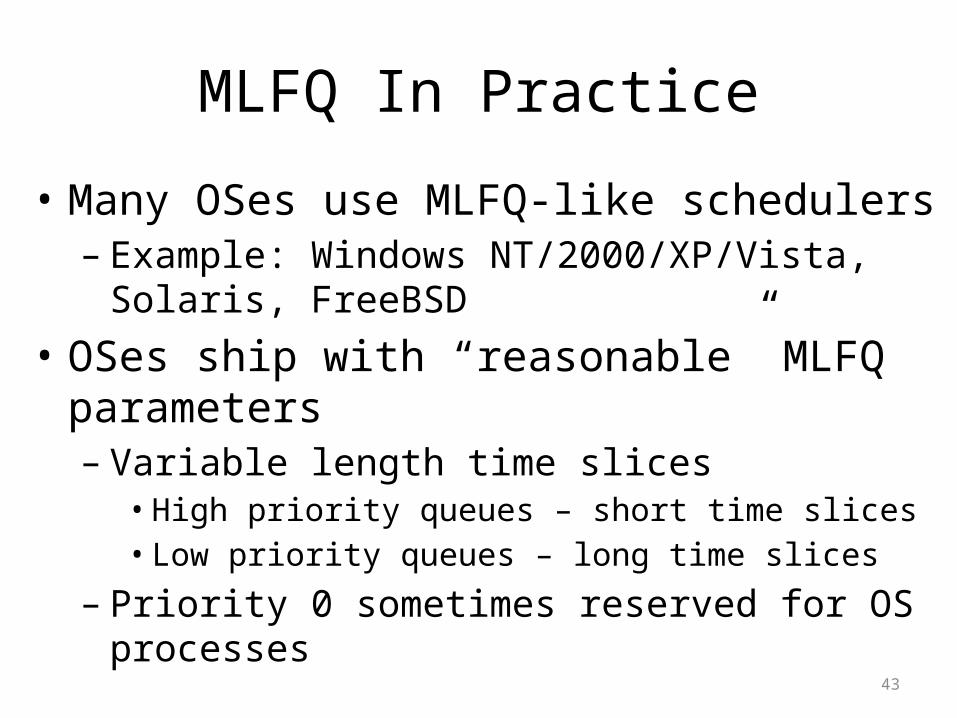
MLFQ In Practice

• Many OSes use MLFQ-like schedulers– Example: Windows NT/2000/XP/Vista, Solaris, FreeBSD

• OSes ship with “reasonable” MLFQ parameters– Variable length time slices• High priority queues – short time slices• Low priority queues – long time slices

– Priority 0 sometimes reserved for OS processes

44

Giving Advice

• Some OSes allow users/processes to give the scheduler “hints” about priorities

• Example: nice command on Linux$ nice <options> <command [args …]>– Run the command at the specified priority– Priorities range from -20 (high) to 19 (low)

45


46

Status Check

• Thus far, we have examined schedulers designed to optimize performance– Minimum response times– Minimum turnaround times

• MLFQ achieves these goals, but it’s complicated– Non-trivial to implement– Challenging to parameterize and tune

• What about a simple algorithm that achieves fairness?

47

Lottery Scheduling• Key idea: give each process a bunch of tickets– Each time slice, scheduler holds a lottery– Process holding the winning ticket gets to run

• Probabilistic scheduling– Over time, run time for each process converges to the

correct value (i.e. the # of tickets it holds)

Process Arrival Time Ticket Range

P1 0 0-74 (75 total)

P2 0 75-99 (25 total)

P1 P2 P1 P1 P1 P2 P2 P1Time: 0 2 4 6 8 10 12 14 16 20

P1 P1 P118 22

• P1 ran 8 of 11 slices – 72%• P2 ran 3 of 11 slices – 27%

Implementation Advantages• Very fast scheduler execution– All the scheduler needs to do is run random()– No need to manage O(log N) priority queues

• No need to store lots of state– Scheduler needs to know the total number of tickets– No need to track process behavior or history

• Automatically balances CPU time across processes– New processes get some tickets, adjust the overall size of the

ticket pool• Easy to prioritize processes– Give high priority processes many tickets– Give low priority processes a few tickets– Priorities can change via ticket inflation (i.e. minting tickets)

49

Is Lottery Scheduling Fair?

• Does lottery scheduling achieve fairness?– Assume two processes

with equal tickets– Runtime of processes

varies– Unfairness ratio = 1 if

both processes finish at the same time

Unfair to short job due to randomness

Randomness is amortized over long

time scales

50

Stride Scheduling

• Randomness is lets us build a simple and approximately fair scheduler– But fairness is not guaranteed

• Why not build a deterministic, fair scheduler?• Stride scheduling– Each process is given some tickets– Each process has a stride = a big # / # of tickets– Each time a process runs, its pass += stride– Scheduler chooses process with the lowest pass to

run next

51

Stride Scheduling ExampleProcess Arrival

TimeTickets Stride

(K = 10000)P1 0 100 100

P2 0 50 200

P3 0 250 40

P1 pass

P2 pass

P3 pass

Who runs?

0 0 0 P1

100 0 0 P2

100 200 0 P3

100 200 40 P3

100 200 80 P3

100 200 120 P1

200 200 120 P3

200 200 160 P3

200 200 200 …

• P1 ran 2 of 8 slices – 25%• P2 ran 1 of 8 slices – 12.5%• P3 ran 5 of 8 slices – 62.5%

• P1: 100 of 400 tickets – 25%• P2: 50 of 400 tickets – 12.5%• P3: 250 of 400 tickets – 62.5%

52

Lingering Issues

• Why choose lottery over stride scheduling?– Stride schedulers need to store a lot more state– How does a stride scheduler deal with new processes?• Pass = 0, will dominate CPU until it catches up

• Both schedulers require tickets assignment– How do you know how many tickets to assign to each

process?– This is an open problem

53


54

Status Check

• Thus far, all of our schedulers have assumed a single CPU core

• What about systems with multiple CPUs?– Things get a lot more complicated when the

number of CPUs > 1

55

Symmetric Multiprocessing (SMP)

• ≥2 homogeneous processors– May be in separate physical packages

• Shared main memory and system bus• Single OS that treats all processors equally

Main Memory

System Bus

L1 Cache

Core

L1 Cache

Core

CPU 1

L2 Cache

L1 Cache

Core

L1 Cache

Core

CPU 2

L2 Cache

56

Hyperthreading

• Two threads on a single CPU core

Non-HyperthreadedCore

HyperthreadedCore

Thread 1 CPU Busy Memory Stall CPU Busy Memory

Stall

Thread 2 CPU BusyCPU Busy Memory Stall

Thread 1 CPU Busy Memory Stall CPU Busy Memory

Stall

57

Brief Intro to CPU Caches

Main Memory

System Bus

L1 Cache

Core

L1 Cache

Core

CPU 1

L2 Cache

L1 Cache

Core

L1 Cache

Core

CPU 2

L2 Cache

P1 Data

P2 Data

P3 Data

P1

P1

P1

P2

P2

P2

P3

P3

P3

P1

P1

Memory fetches are slow :(

Cache hits are fast :)

P1 has fast access to P2’s data

… but access to P3’s data is slow

• Process performance is linked to locality– Ideally, a process should be placed close to its data

• Shared data is problematic due to cache coherency– P3 writes variable x, new value is cached in CPU 2– P2 in CPU 1 reads x, but value in main memory is stale

58

NUMA and Affinity• Non-Uniform Memory Access (NUMA) architecture– Memory access time depends on the location of the data

relative to the requesting process• Leads to cache affinity– Ideally, processes want to stay close to their cached data

CPU 1 P1

P2

P3

CPU 2

59

CPU 0

CPU 1

CPU 2

CPU 3

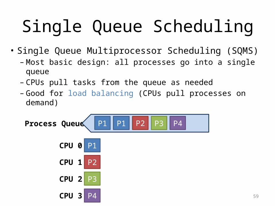
Single Queue Scheduling• Single Queue Multiprocessor Scheduling (SQMS)– Most basic design: all processes go into a single queue– CPUs pull tasks from the queue as needed– Good for load balancing (CPUs pull processes on

demand)Process Queue P1 P2 P3 P4 P5

P1

P2

P3

P4

P1 P2 P3 P4

60

Problems with SQMS

• The process queue is a shared data structure– Necessitates locking, or careful lock-free design

• SQMS does not respect cache affinity

CPU 0

CPU 1

CPU 2

CPU 3

Process Queue P1 P2 P3 P4 P5

P1

P2

P3

P4

P1 P2 P3 P4

P5

P1

P2

P3

P5 P1 P2 P3

P4

P5

P1

P2

Time

P4 P5 P1 P2

P3

P4

P5

P1

Worst case scenario: processes rarely run

on the same CPU

61

Multi-Queue Scheduling

• SQMS can be modified to preserve affinity• Multiple Queue Multiprocessor Scheduling (MQMS)– Each CPU maintains it’s own queue of processes– CPUs schedule their processes independently

CPU 0

CPU 1

Queue 0 P1

P2

P3

P4

P1

P2

P3

P4

P1

P2Queue 1

62

CPU 0

CPU 1

Queue 0

Queue 1

Advantages of MQMS

• Very little shared data– Queues are (mostly) independent

• Respects cache affinity

P1

P2

P3

P4

P1

P2

P3

P4

P1

P2

Time

P3

P4

P1

P2

63

Shortcoming of MQMS

• MQMS is prone to load imbalance due to:– Different number of processes per CPU– Variable behavior across processes

• Must be dealt with through process migration

Queue 0

Queue 1

P1

P4P2

CPU 0

CPU 1

P1

P2 P4

Time

P1

P2

…

Idle the CPU?

CPU 0

CPU 1

P1

P2 P4

Time

P2

Unfair CPU Usage?

64

Strategies for Process Migration• Push migration

• Pull migration, a.k.a. work stealing

CPU 0 / Queue 0

CPU 1 / Queue 1

P1

P2 P4 P3“I have too many

processes, take one”

CPU 0 / Queue 0

CPU 1 / Queue 1

P1

P2 P4 P3

“I don’t have enough processes, give me one”

65


66

Final Status Check• At this point, we have looked at many:– Scheduling algorithms– Types of processes (CPU vs. I/O bound)– Hardware configurations (SMP)

• What do real OSes do?• Case study on the Linux kernel– Old scheduler: O(1)– Current scheduler: Completely Fair Scheduler (CFS)– Alternative scheduler: BF Scheduler (BFS)

67

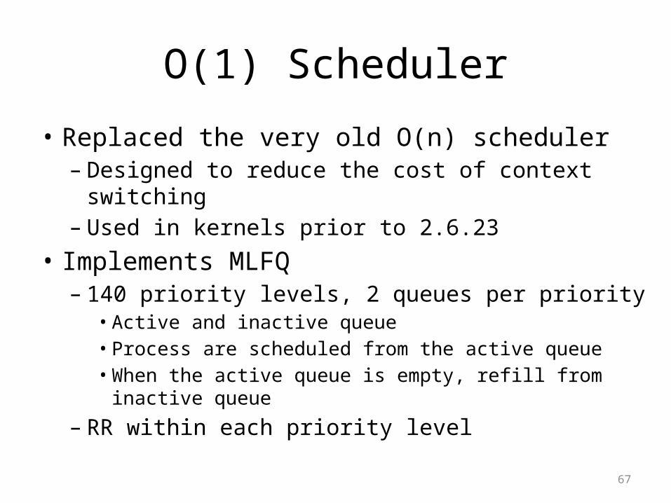
O(1) Scheduler

• Replaced the very old O(n) scheduler– Designed to reduce the cost of context switching– Used in kernels prior to 2.6.23

• Implements MLFQ– 140 priority levels, 2 queues per priority• Active and inactive queue• Process are scheduled from the active queue• When the active queue is empty, refill from inactive queue

– RR within each priority level

68

Priority Assignment

• Static priorities – nice values [-20,19]– Default = 0– Used for time slice calculation

• Dynamic priorities [0, 139]– Used to demote CPU bound processes– Maintain high priorities for interactive processes– sleep() time for each process is measured• High sleep time interactive or I/O bound high priority

69

SNP / NUMA Support

• Processes are placed into a virtual hierarchy– Groups are scheduled onto a physical CPU– Processes are preferentially pinned to individual

cores• Work stealing used for load balancing

70

Completely Fair Scheduler (CFS)• Replaced the O(1) scheduler– In use since 2.6.23, has O(log N) runtime

• Moves from MLFQ to Weighted Fair Queuing– First major OS to use a fair scheduling algorithm– Very similar to stride scheduling– Processes ordered by the amount of CPU time they use

• Gets rid of active/inactive run queues in favor of a red-black tree of processes

• CFS isn’t actually “completely fair”– Unfairness is bounded O(N)

71

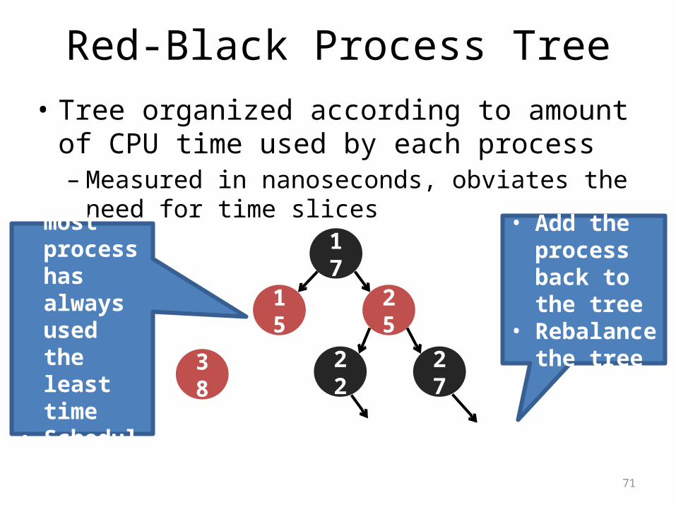
Red-Black Process Tree• Tree organized according to amount of CPU

time used by each process– Measured in nanoseconds, obviates the need for

time slices17

15 25

22 27

• Left-most process has always used the least time

• Scheduled next

38

• Add the process back to the tree

• Rebalance the tree

72

BF Scheduler• What does BF stand for?– Look it up yourself

• Alternative to CFS, introduced in 2009– O(n) runtime, single run queue– Dead simple implementation

• Goal: a simple scheduling algorithm with fewer parameters that need manual tuning– Designed for light NUMA workloads– Doesn’t scale to cores > 16

• For the adventurous: download the BFS patches and build yourself a custom kernel

cs 5600 computer systems lecture 6: process scheduling

Documents