CS 4700:Foundations of Artificial Intelligence

Bart Selman

Search TechniquesR&N: Chapter 3

Outline

Search: tree search and graph search

Uninformed search: very briefly (covered before in other pre-requisite courses – recommendation: review these techniques at home)

Informed search ß focus of the lecture

Uninformed search strategies

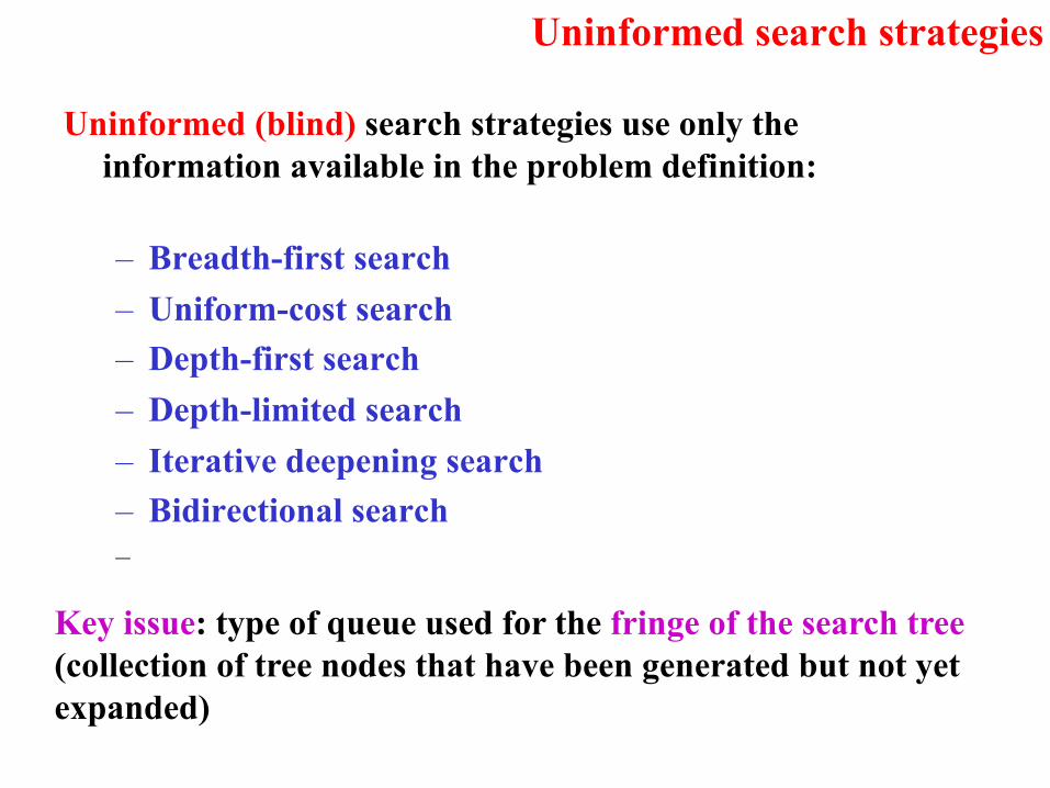
Uninformed (blind) search strategies use only the information available in the problem definition:

– Breadth-first search– Uniform-cost search– Depth-first search– Depth-limited search– Iterative deepening search– Bidirectional search–

Key issue: type of queue used for the fringe of the search tree(collection of tree nodes that have been generated but not yet expanded)

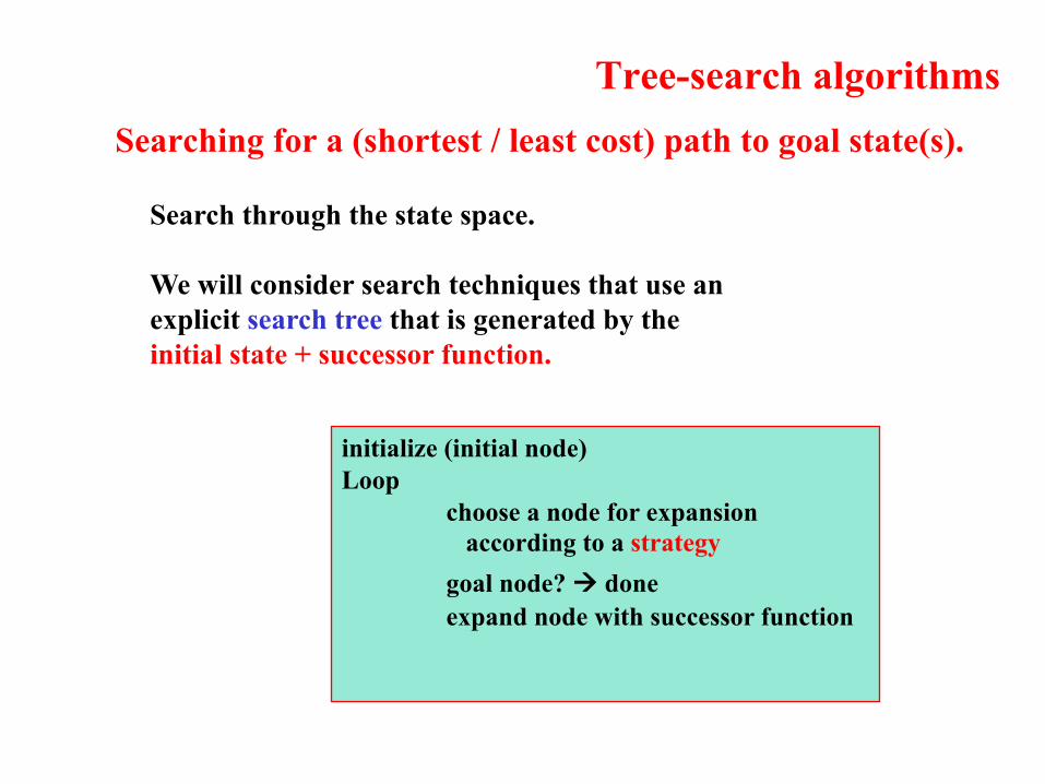
Searching for a (shortest / least cost) path to goal state(s).

Search through the state space.

We will consider search techniques that use an explicit search tree that is generated by the initial state + successor function.

initialize (initial node)Loop

choose a node for expansion according to a strategy

goal node? à doneexpand node with successor function

Tree-search algorithms

Tree search exampleNode selectedfor expansion.

Nodes added to tree.

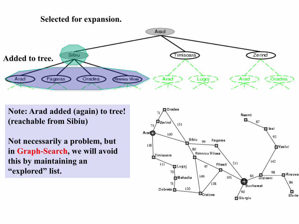
Selected for expansion.

Added to tree.

Note: Arad added (again) to tree!(reachable from Sibiu)

Not necessarily a problem, butin Graph-Search, we will avoidthis by maintaining an“explored” list.

Tree-search algorithms

Basic idea:– simulated exploration of state space by generating successors of

already-explored states (a.k.a. ~ expanding states)–

Note: 1) Here we only check a node for possibly being a goal state, after we select the node for expansion. 2) A “node” is a data structure containing state + additional info (parentnode, etc.

Fig. 3.7 R&N, p. 77

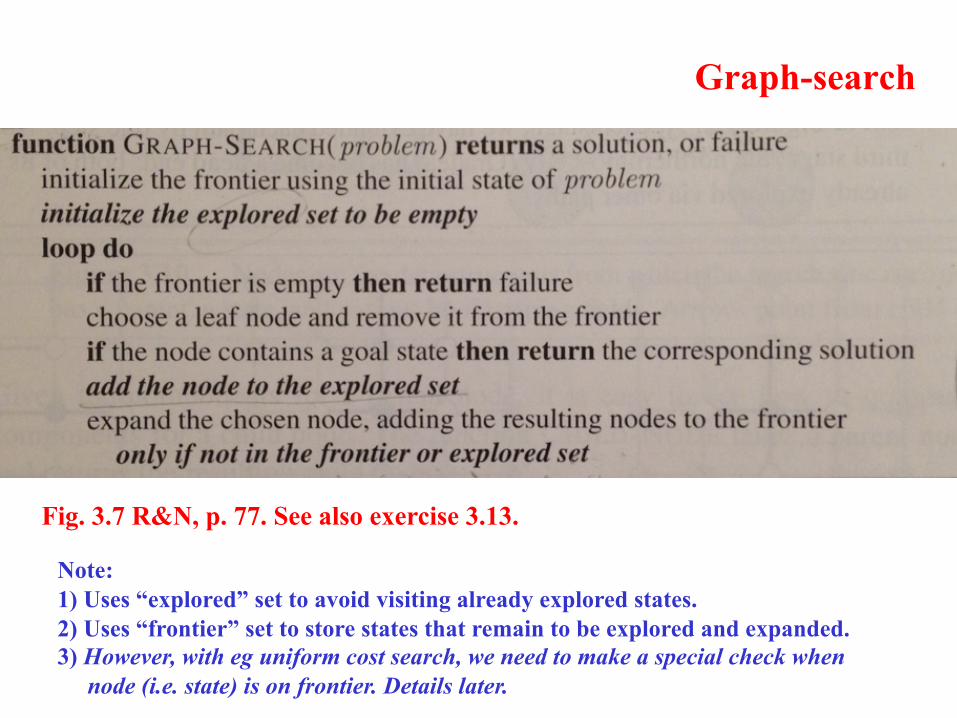
Graph-search

Note: 1) Uses “explored” set to avoid visiting already explored states.2) Uses “frontier” set to store states that remain to be explored and expanded.3) However, with eg uniform cost search, we need to make a special check when

node (i.e. state) is on frontier. Details later.

Fig. 3.7 R&N, p. 77. See also exercise 3.13.

Search strategies

A search strategy is defined by picking the order of node expansion.

Strategies are evaluated along the following dimensions:– completeness: does it always find a solution if one exists?– time complexity: number of nodes generated– space complexity: maximum number of nodes in memory– optimality: does it always find a least-cost solution?–

Time and space complexity are measured in terms of – b: maximum branching factor of the search tree– d: depth of the least-cost solution– m: maximum depth of the state space (may be ∞)–

Uninformed search strategies

Uninformed (blind) search strategies use only the information available in the problem definition:

– Breadth-first search– Uniform-cost search– Depth-first search– Depth-limited search– Iterative deepening search– Bidirectional search–

Key issue: type of queue used for the fringe of the search tree(collection of tree nodes that have been generated but not yet expanded)

Breadth-first search

Expand shallowest unexpanded node.

Implementation:– fringe is a FIFO queue, i.e., new nodes go at end

(First In First Out queue.)Fringe queue: <A>

Select A fromqueue and expand.

Gives<B, C>

Queue: <B, C>

Select B fromfront, and expand.

Put children at theend.

Gives<C, D, E>

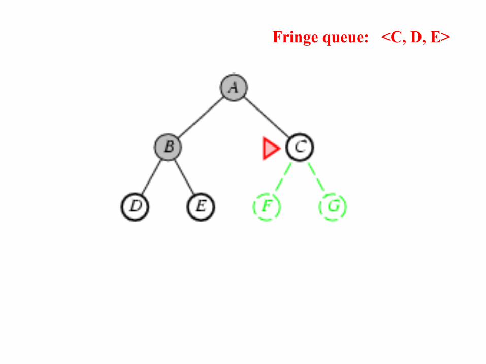
Fringe queue: <C, D, E>

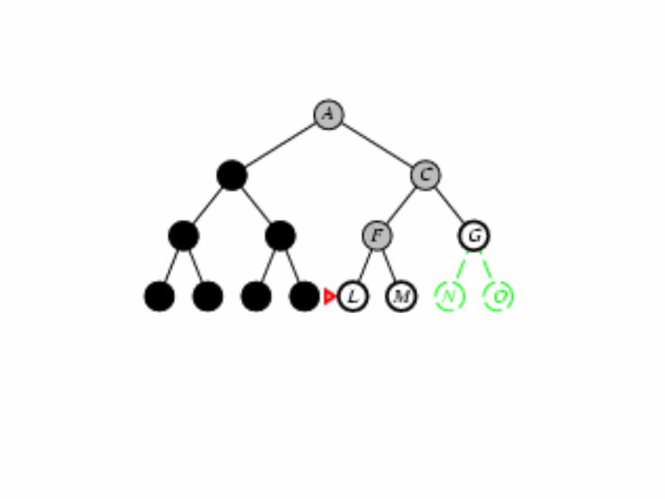
Fringe queue: <D, E, F, G>

Assuming no further children, queue becomes<E, F, G>, <F, G>, <G>, <>. Each time node checkedfor goal state.

Properties of breadth-first search(check them at home!!!!)

Complete? Yes (if b is finite)

Time? 1+b+b2+b3+… +bd + b(bd-1) = O(bd+1)

Space? O(bd+1) (keeps every node in memory;needed also to reconstruct soln. path)

Optimal soln. found?Yes (if all step costs are identical)

Space is the bigger problem (more than time)

b: maximum branching factor of the search treed: depth of the least-cost solution

Note: check for goal only whennode is expanded.

Depth d, goal may be last node (only checked when expanded.).

Uniform Cost

We factor in the cost of each step (e.g., distance form current state to the neighbors). Assumption: costs are non-negative.

g(n) = cost so far to reach n

Queue à ordered by cost

If all the steps are the same à breadth-first search is optimal since it always expands the shallowest (least cost)!

Uniform-cost search à expand first the nodes with lowest cost (instead of depth).

Does it ring a bell?

Uniform-cost searchTwo subtleties: (bottom p. 83 Norvig)1) Do goal state test, only when a node is selected for expansion.

(Reason: Bucharest may occur on frontier with a longer thanoptimal path. It won’t be selected for expansion yet. Other nodeswill be expanded first, leading us to uncover a shorter path toBucharest. See also point 2).

2) Graph-search alg. says “don’t add child node to frontier if already onexplored list or already on frontier.” BUT, child may give a shorter pathto a state already on frontier. Then, we need to modify the existingnode on frontier with the shorter path. See fig. 3.14 (else-if part).

Uniform-cost search

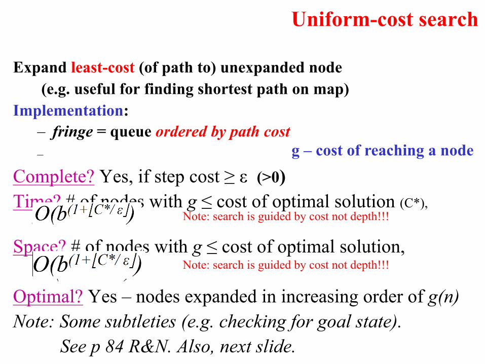
Expand least-cost (of path to) unexpanded node (e.g. useful for finding shortest path on map)

Implementation:– fringe = queue ordered by path cost–

Complete? Yes, if step cost ≥ ε (>0)Time? # of nodes with g ≤ cost of optimal solution (C*),

O(b(1+ëC*/ εû)Space? # of nodes with g ≤ cost of optimal solution,

O(b(1+ëC*/ εû)Optimal? Yes – nodes expanded in increasing order of g(n)Note: Some subtleties (e.g. checking for goal state).

See p 84 R&N. Also, next slide.

g – cost of reaching a node

Note: search is guided by cost not depth!!!

Note: search is guided by cost not depth!!!

Depth-first search“Expand deepest unexpanded node”

Implementation:– fringe = LIFO queue, i.e., put successors at front (“push on stack”)

Last In First Out

Fringe stack:A

Expanding A, gives stack:

BC

So, B next.

Expanding B, gives stack:

DEC

So, D next.

Expanding D, gives stack:

HIEC

So, H next.etc.

What is main advantage over breadth first search?

What information is stored? How much storage required?

The stack. O(depth x branching).

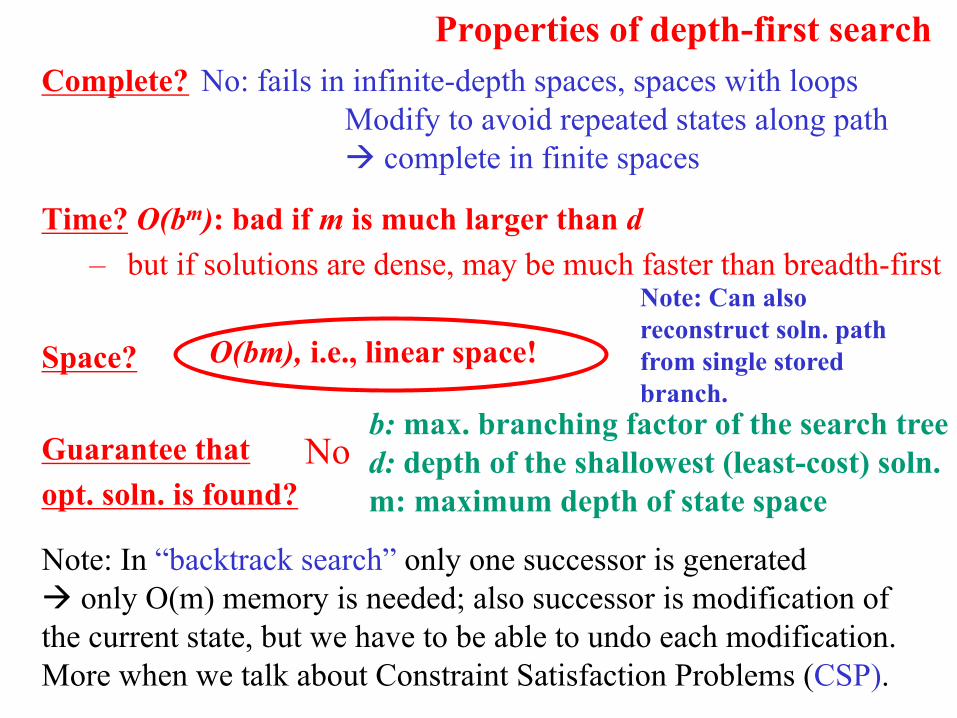
Properties of depth-first searchComplete?

Time? O(bm): bad if m is much larger than d– but if solutions are dense, may be much faster than breadth-first

Space?

Guarantee thatopt. soln. is found?

Note: In “backtrack search” only one successor is generated à only O(m) memory is needed; also successor is modification ofthe current state, but we have to be able to undo each modification.More when we talk about Constraint Satisfaction Problems (CSP).

b: max. branching factor of the search treed: depth of the shallowest (least-cost) soln.m: maximum depth of state space

No: fails in infinite-depth spaces, spaces with loopsModify to avoid repeated states along pathà complete in finite spaces

O(bm), i.e., linear space!

No

Note: Can also reconstruct soln. path from single stored branch.

Iterative deepening search l =0

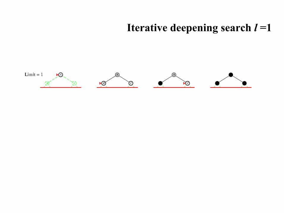
Iterative deepening search l =1

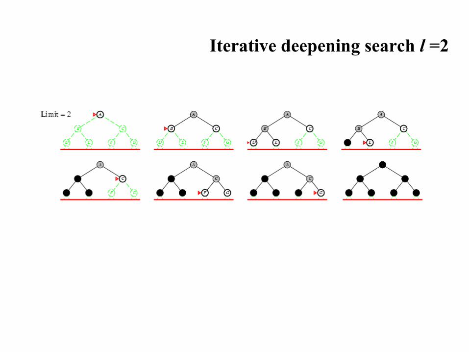
Iterative deepening search l =2

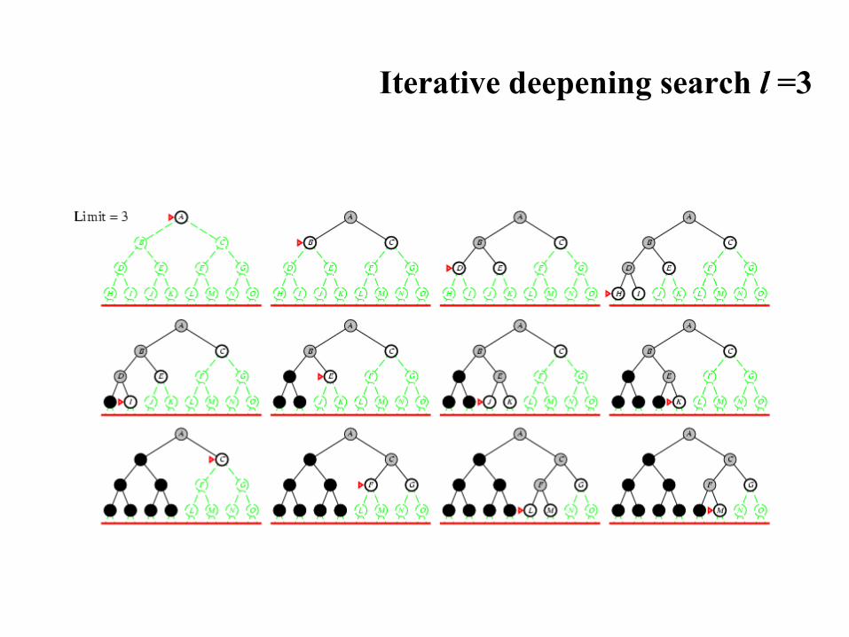
Iterative deepening search l =3

Combine good memory requirements of depth-first withthe completeness of breadth-first when branching factor isfinite and is optimal when the path cost is a non-decreasing

function of the depth of the node.

Why would one do that?

Idea was a breakthrough in game playing. All gametree search uses iterative deepening nowadays. What’sthe added advantage in games?

“Anytime” nature.

Iterative deepening search

Iterative deepening search

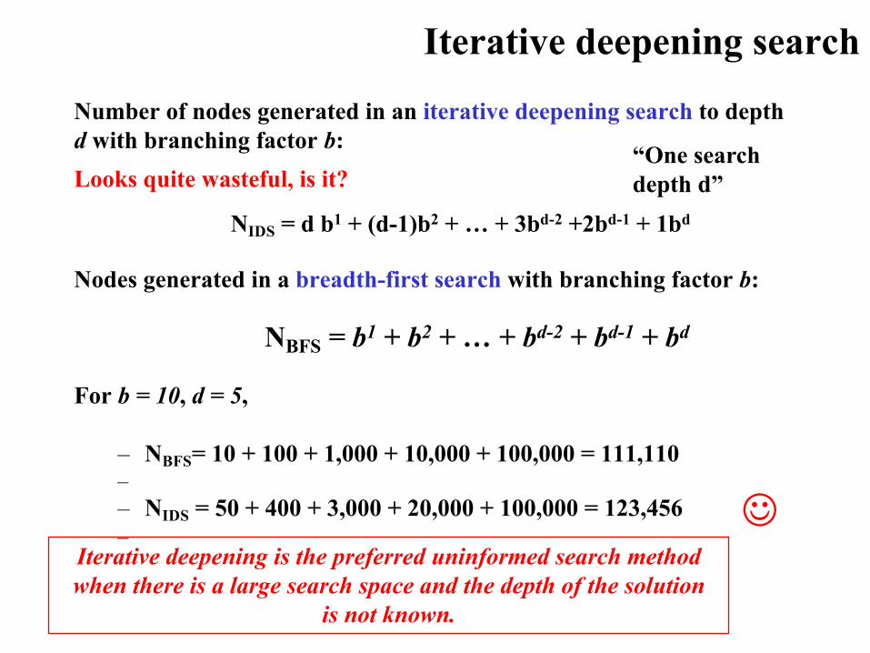
Number of nodes generated in an iterative deepening search to depthd with branching factor b:

NIDS = d b1 + (d-1)b2 + … + 3bd-2 +2bd-1 + 1bd

Nodes generated in a breadth-first search with branching factor b:

NBFS = b1 + b2 + … + bd-2 + bd-1 + bd

For b = 10, d = 5,

– NBFS= 10 + 100 + 1,000 + 10,000 + 100,000 = 111,110–– NIDS = 50 + 400 + 3,000 + 20,000 + 100,000 = 123,456–

Looks quite wasteful, is it?

Iterative deepening is the preferred uninformed search methodwhen there is a large search space and the depth of the solution

is not known.

J

“One searchdepth d”

Properties of iterative deepening search

Complete? Yes(b finite)

Time? d b1 + (d-1)b2 + … + bd = O(bd)

Space? O(bd)

Optimal? Yes, if step costs identical

Bidirectional Search• Simultaneously:

– Search forward from start– Search backward from the goal

Stop when the two searches meet.

• If branching factor = b in each direction,with solution at depth d è only O(2 bd/2)= O(2 bd/2)

• Checking a node for membership in the other search tree can be done in constant time (hash table)

• Key limitations:Space O(bd/2) Also, how to search backwards can be an issue (e.g., in Chess)? What’s tricky?Problem: lots of states satisfy the goal; don’t know which one is relevant.

Aside: The predecessor of a node should be easily computable (i.e., actions are easily reversible).

Repeated statesFailure to detect repeated states can turn linear problem into an exponential one!

Problems in which actions are reversible (e.g., routing problems orsliding-blocks puzzle). Also, in eg Chess; uses hash tables to checkfor repeated states. Huge tables 100M+ size but very useful.

See Tree-Search vs. Graph-Search in Fig. 3.7 R&N. But need tobe careful to maintain (path) optimality and completeness.

Summary: General, uninformed searchOriginal search ideas in AI where inspired by studies of human problem

solving in, eg, puzzles, math, and games, but a great many AI tasks now require some form of search (e.g. find optimal agent strategy; active learning; constraint reasoning; NP-complete problems require search).

Problem formulation usually requires abstracting away real-world details to define a state space that can feasibly be explored.

Variety of uninformed search strategies

Iterative deepening search uses only linear space and not much more time than other uninformed algorithms.

Avoid repeating states / cycles.

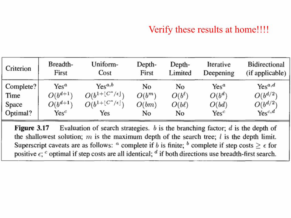
Verify these results at home!!!!