04/19/23 1

CS 367: Model-Based ReasoningLecture 15 (03/12/2002)

Gautam Biswas

04/19/23 2

Today’s Lecture

Last Lectures: Modeling with Bond Graphs

Today’s Lecture: Review Bond Graphs and Causality State Space Equations from Bond Graphs More Complex Examples 20-SIM

04/19/23 3

Review: Modeling with Bond Graphs

• Based on concept of reticulation• Properties of system lumped into processes with distinct

parameter valuesLumped Parameter Modeling

• Dynamic System Behavior: function of energy exchange between components

• State of physical system – defined by distribution of

energy at any particular timeDynamic Behavior: Current State + Energy exchange

mechanisms

04/19/23 4

Review: Modeling with Bond Graphs

Exchange of energy in system through ports 1 ports: C, I: energy storage elements; R: dissipator 2 ports: TF, GY Exchange with environment: through sources and sinks:

Se & Sf

Behavior Generation: two primary principles Continuity of power Conservation of energy

enforced at junctions: 3 ports

0- (parallel) junction

1- (series) junction

04/19/23 5

Review: Junctions

Electrical Domain: 0- enforces Kirchoff’s current law, 1- enforces Kirchoff’s voltage lawMechanical Domain: 0- enforces geometric compatibility of single force + set of velocities that must sum to 0; 1- enforces dynamic equilibrium of forces associated with a single velocityHydraulic Domain: 0- conservation of volume flow rate, when a set of pipes join1- sum of pressure drops across a circuit (loop) involving a single flow must sum to 0.

Sometimes junction structures are not obvious.

04/19/23 6

Component Behaviors

Mechanics Electricity Hydraulic Thermal

Effort e(t) F, force V, voltage P, pressure T, temperature

Flow f(t) v, velocity i, current Q, volume flow rate

, heat flow

rate

Momentum p =e.dt P, momentum

, flux p =P.dt P.dt = Pp

Displacement q =f.dt x, distance q, charge q =Q.dt

volume

Q, heat energy

Power P(t)=e(t).f(t) F(t).v(t) V(t).i(t) P(t).Q(t)

Energy E(p)=f.dp

E(q)=e.dq

v.dP (kinetic)

F.dx (potential)

i.d v.dq

Q.dp

P.dq

Q

Q

Q

04/19/23 7

Building Electrical Models

For each node in circuit with a distinct potential create a 0-junctionInsert each 1 port circuit element by adjoining it to a 1-junction and inserting the 1-junction between the appropriate of 0-junctions.Assign power directions to bondsIf explicit ground potential, delete corresponding 0-junction and its adjacent bondsSimplify bond graph (remove extraneous junctions)

Hydraulic, thermal systems similar, but mechanical different

04/19/23 8

Electrical Circuit: Example

04/19/23 9

Electrical Circuits: Example 2

Try this one:

04/19/23 10

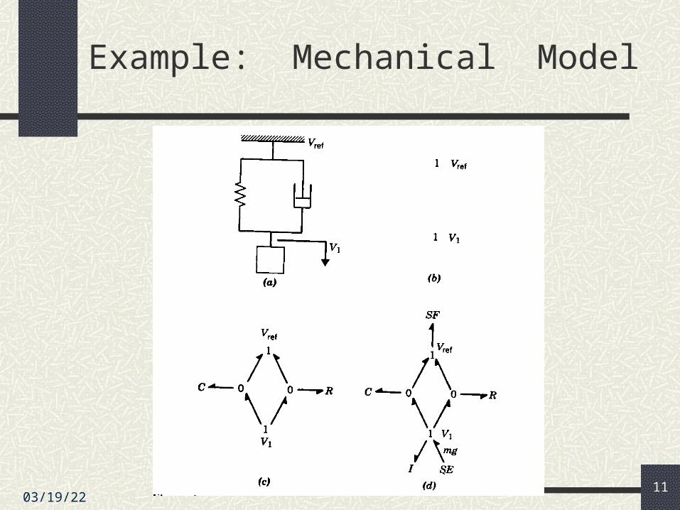
Building Mechanical Models

For each distinct velocity, establish a 1-junction (consider both absolute and relative velocities)Insert the 1-port force-generating elements between appropriate pairs of 1-junctions; using 0-junctions;also add inertias to respective 1-junctions (be sure they are properly defined wrt inertial frame)Assign power directionsEliminate 0 velocity 1-junctions and their bondsSimplify bond graph

04/19/23 11

Example: Mechanical Model

04/19/23 12

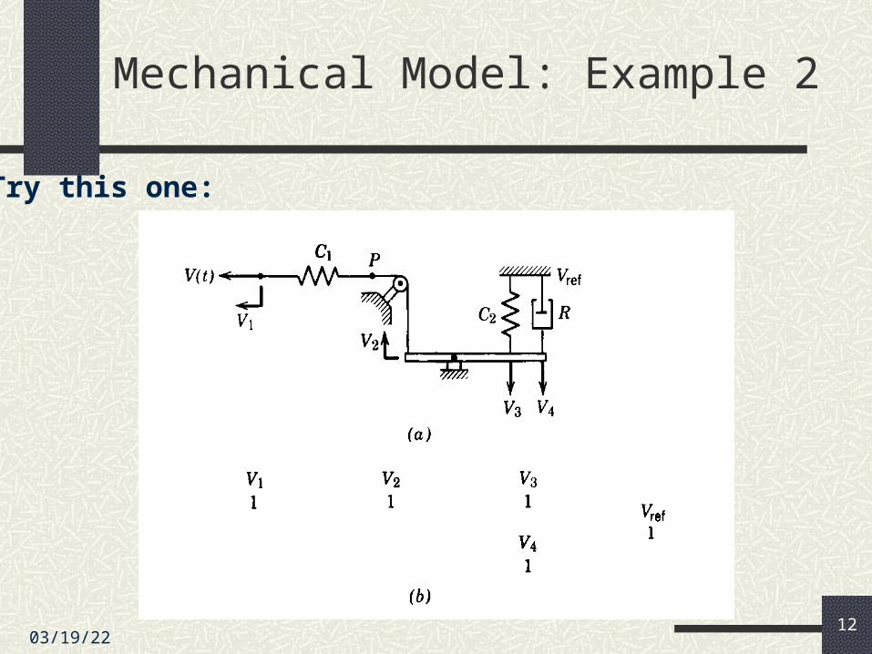
Mechanical Model: Example 2

Try this one:

04/19/23 13

Behavior of System: State Space Equations

Linear System

Nonlinear System

vectoroutputpyuDxCy

vectorinputmu

vectorstatenxuBxAx

1:..

1:

1:;..

vectoroutputpyuxy

vectorinputmu

vectorstatenxuxx

1:),(

1:

1:;),(

04/19/23 14

State Equations

Linear

Nonlinear

mnmnnnnnn

mmnn

mmnn

ububxaxax

ububxaxax

ububxaxax

uBxAx

.........

.

..

.........

.........

..

1111

212121212

111111111

),( uxx

),....,,,....,(

.

..

),....,,,....,(

),....,,,....,(

11

1122

1111

mnnn

mn

mn

uuxxx

uuxxx

uuxxx

04/19/23 15

State Space: Standard form

vx

k.xb.vvm.

vandxvariablesstateoftermsinWrite

Or

xkxbxm

xbxkxm

0...

...

Single nth order form

n first-order coupled equations

In general, can have any combination in between

04/19/23 16

More complex example

g

gmm

kxmm

kkx

dt

d

mmk

m

kx

dt

d

variablesystemasxwithformorderFourth24

)11

(..

.)()

11()(

2112

21

212

211

2

22

2

04/19/23 17

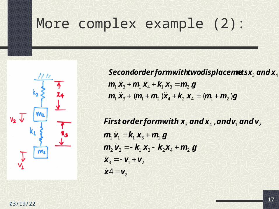
More complex example (2):

gmmxkxmmxm

gmxkxmxm

xandxntsdisplacemetwowithformorderSecond

)(.)(.

....

214242131

2314131

43

2

213

2423122

13111

2143

4

...

...

,

vx

vvx

gmxkxkvm

gmxkvm

vandvandxandxwithformorderFirst

04/19/23 18

Causality in Bond Graphs

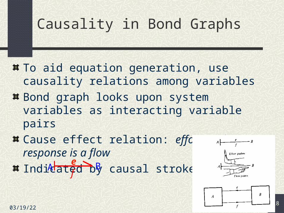
To aid equation generation, use causality relations among variables

Bond graph looks upon system variables as interacting variable pairs

Cause effect relation: effort pushes, response is a flow

Indicated by causal stroke on a bond

Bef

A

04/19/23 19

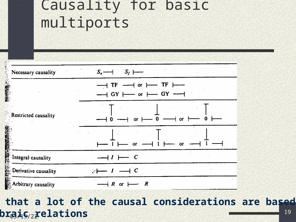
Causality for basic multiports

Note that a lot of the causal considerations are based onalgebraic relations

04/19/23 20

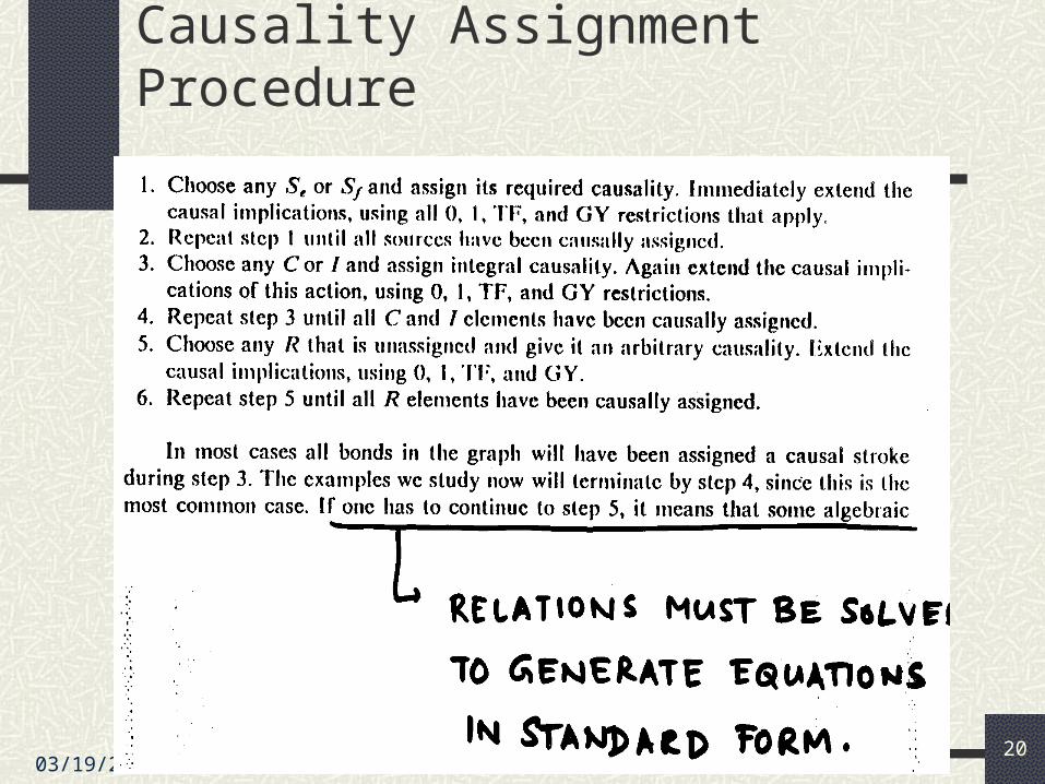
Causality Assignment Procedure

04/19/23 21

Causality Assignment: Example

04/19/23 22

Causality Assignment: Double Oscillator

04/19/23 23

Causality Assignment: Example 3

Try this one:

04/19/23 24

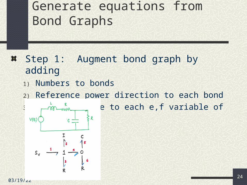
Generate equations from Bond Graphs

Step 1: Augment bond graph by adding1) Numbers to bonds

2) Reference power direction to each bond

3) A causal sense to each e,f variable of bond

04/19/23 25

Equation generation procedure

04/19/23 26

Equation generation example

65

5

2

2

6

5

2

2

6

62645

5

5.

533432

.

)(

.)()(

2

23

RC

q

I

p

R

e

I

p

R

efffq

C

qtE

efRtEeetEp

IPR

04/19/23 27

Equation Generation: Example 2

04/19/23 28

H. W. Problem 1 :

Two springs, masses, & damper friction all linear.

F0(t) = f1 = constant.

Build bond graph; state equations.

Simulate for various parameter values.

m1 m2

k1 F0(t)

k2

b1 b2

04/19/23 29

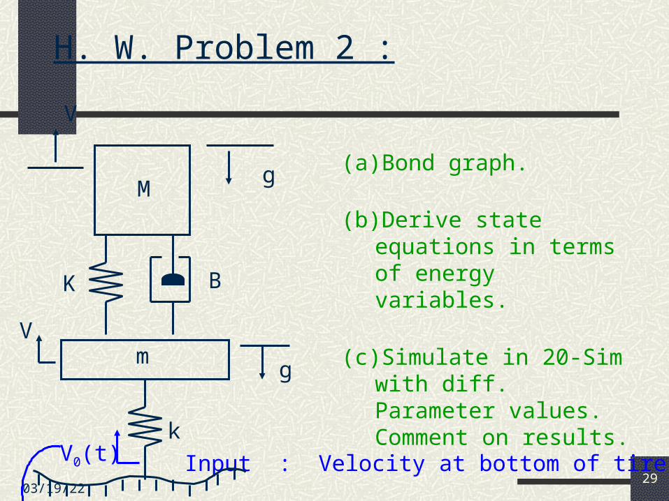
H. W. Problem 2 :

Input : Velocity at bottom of tire

(a) Bond graph.

(b) Derive state equations in terms of energy variables.

(c) Simulate in 20-Sim with diff. Parameter values. Comment on results.

V

g

K B

V

g

kV0(t)

M

m

04/19/23 30

Extending Modeling to other domains

Fluid Systems e(t) – Pressure, P(t) f(t) – Volume flow rate, Q(t) Momentum, p = e.dt = Pp, integral of pressure Displacement, q = Q.dt = V, volume of flow Power, P(t).Q(t) Energy (kinetic): Q(t).dPp Energy (potential): P(t).dVFluid Port: a place where we can define an average pressure, P and a

volume flow rate, QExamples of ports: (i) end of a pipe or tube

(ii) threaded hole in a hydraulic pump

04/19/23 31

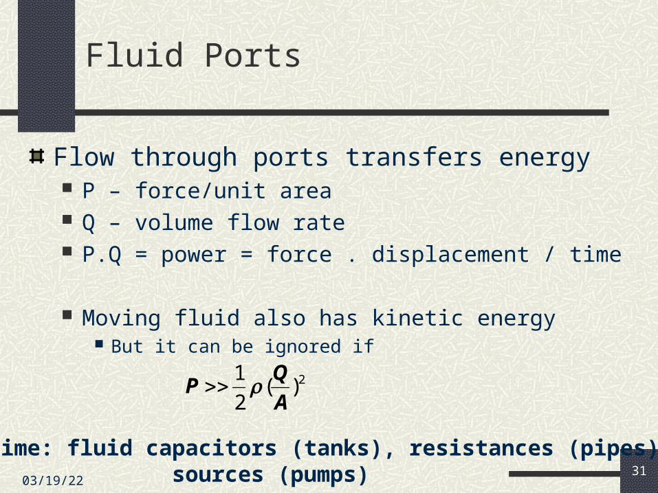
Fluid Ports

Flow through ports transfers energy P – force/unit area Q – volume flow rate P.Q = power = force . displacement / time

Moving fluid also has kinetic energy But it can be ignored if

2)(2

1

A

QP

Next time: fluid capacitors (tanks), resistances (pipes), and sources (pumps)