cs 277, data mining web data analysis: part 2,...
TRANSCRIPT
CS 277, Data Mining Web Data Analysis: Part 2, Advertising
Padhraic Smyth Department of Computer Science Bren School of Information and Computer Sciences University of California, Irvine
Padhraic Smyth, UC Irvine: CS 277, Winter 2014
3
Internet Advertising, Bids, and Auctions
Padhraic Smyth, UC Irvine: CS 277, Winter 2014
4
“Computational Advertising”
• Revenue of many internet companies is driven by advertising
• Key problem: – Given user data:
• Pages browsed • Keywords used in search • Demographics
– Determine the most relevant ads (in real-time) – About 50% of keyword searches can not be matched effectively to any ads – Other aspects include bidding/pricing of ads
• New research area of “computational advertising” – See link to Stanford class by Andrei Broder on class Web site
Padhraic Smyth, UC Irvine: CS 277, Winter 2014
5
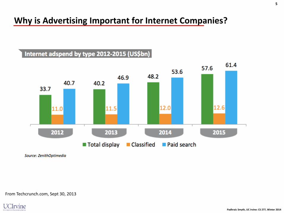
Why is Advertising Important for Internet Companies?
From Techcrunch.com, Sept 30, 2013

Padhraic Smyth, UC Irvine: CS 277, Winter 2014
6
Types of Online Ads
• Display or Banner – Fixed content, usually visual – Or (more recently) video ads
• Sponsored search (Text Ad) – Triggered by search results – Ad selection based on search query terms, user features, click-through rates, ….
• Context-based/Text (Text Ad) – Can be based on content of Web page during browsing – Ad selection based on matching ad content with page content
Padhraic Smyth, UC Irvine: CS 277, Winter 2014
7
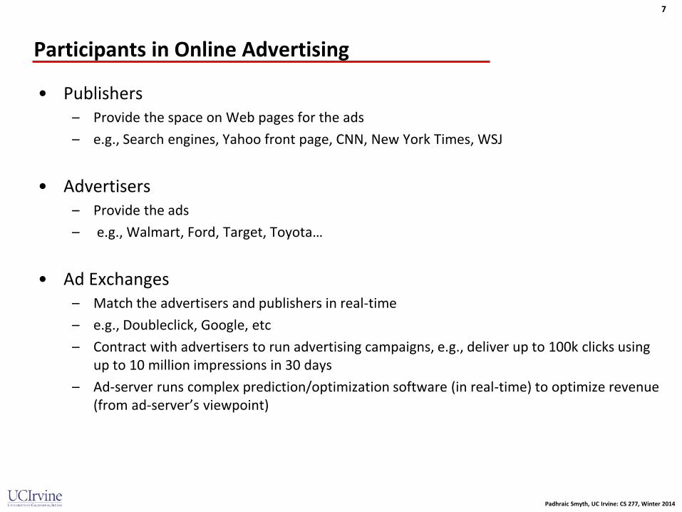
Participants in Online Advertising
• Publishers – Provide the space on Web pages for the ads – e.g., Search engines, Yahoo front page, CNN, New York Times, WSJ
• Advertisers – Provide the ads – e.g., Walmart, Ford, Target, Toyota…
• Ad Exchanges – Match the advertisers and publishers in real-time – e.g., Doubleclick, Google, etc – Contract with advertisers to run advertising campaigns, e.g., deliver up to 100k clicks using
up to 10 million impressions in 30 days – Ad-server runs complex prediction/optimization software (in real-time) to optimize revenue
(from ad-server’s viewpoint)

Padhraic Smyth, UC Irvine: CS 277, Winter 2014
8
Concepts in Online Advertising
• Impression: showing an ad to an online user – CTR = clickthrough rate (typically around 0.1%)
• Revenue mechanisms (to ad-exchange or publisher, from advertiser)
– CPM: cost per 1000 impressions – CPC: cost per click – CPA: cost per action (e.g., customer signs up, makes a purchase..)
• Ad-exchanges and auctions – Impressions can be bid on in real-time in ad-exchanges – Typically a 2nd-price (Vickery) auction – Key to success = accurate prediction of CTR for each impression
Padhraic Smyth, UC Irvine: CS 277, Winter 2014
9
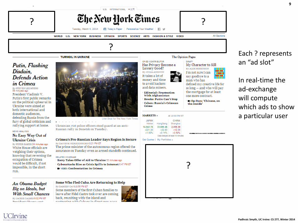
? ?
?
? Each ? represents an “ad slot” In real-time the ad-exchange will compute which ads to show a particular user

Padhraic Smyth, UC Irvine: CS 277, Winter 2014
10
These ads are “impressions”
Padhraic Smyth, UC Irvine: CS 277, Winter 2014
11
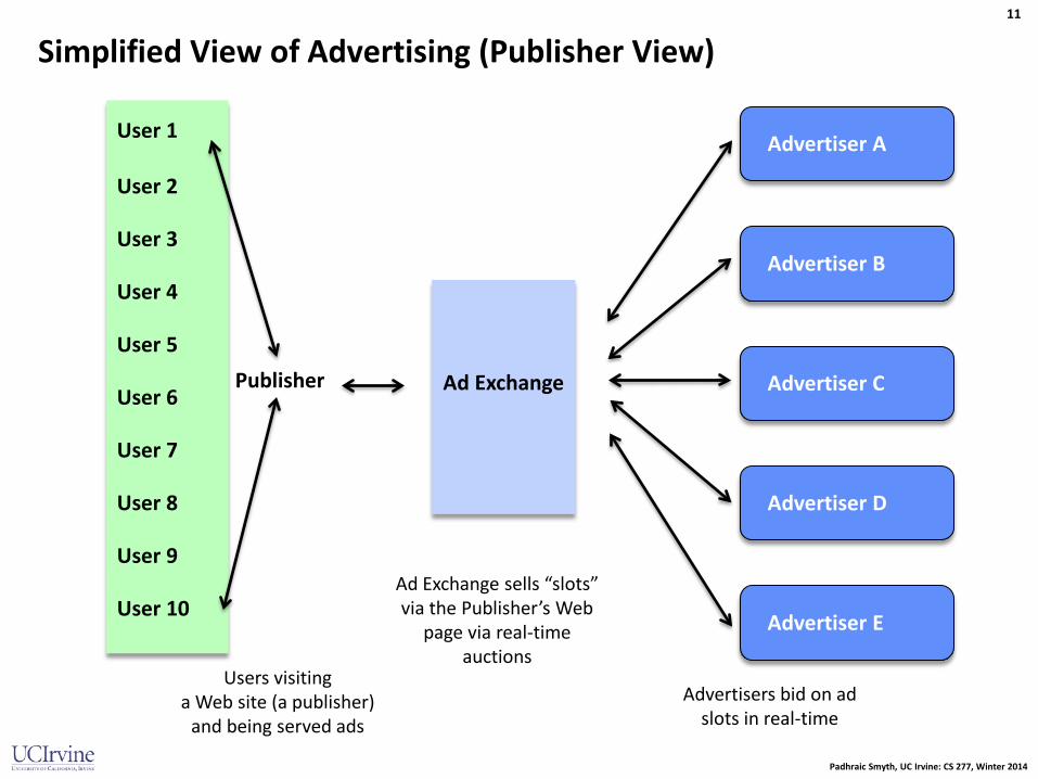
Simplified View of Advertising (Publisher View)
User 1
Publisher
Ad Exchange
Advertiser A
Advertiser 1
Advertiser B
Advertiser C
Advertiser D
Advertiser E
User 2
User 3
User 4
User 5
User 6
User 7
User 8
User 9
User 10
Users visiting a Web site (a publisher)
and being served ads
Ad Exchange sells “slots” via the Publisher’s Web
page via real-time auctions
Advertisers bid on ad slots in real-time

Padhraic Smyth, UC Irvine: CS 277, Winter 2014
12

Padhraic Smyth, UC Irvine: CS 277, Winter 2014
13

Padhraic Smyth, UC Irvine: CS 277, Winter 2014
14
Simplified View of Advertising (Advertiser View)
User 1 Publisher 1
Ad Exchange
Advertiser 1
Advertiser
User 2
User 3
User 4
User 5
User 6
User 7
User 8
Publisher 2
Publisher 3
Publisher 4
Publisher 5
Publisher 6
Users visiting Web sites
(publishers) and being served ads
Publishers selling “inventory” (ad slots) on
an Ad Exchange
An Advertiser making an ad available to be shown
to some set of users

Padhraic Smyth, UC Irvine: CS 277, Winter 2014
15
Padhraic Smyth, UC Irvine: CS 277, Winter 2014
16
Behind the Scenes…
• The previous slides are a very simplified picture of how these systems work……… in practice there are many other factors
• Multiple 3rd party “advertising companies” – In practice rather than just a single “ad exchange” there is a whole “ecosystem” of different
systems and companies that sit between the publisher and the advertisers, optimizing different parts of the ad matching process
• Auction mechanisms – Use of “2nd price auctions”

Padhraic Smyth, UC Irvine: CS 277, Winter 2014
17
Auctions and Bidding for Queries
• Say we have a query (like “flower delivery”)
• Different advertisers can bid to have their ad shown whenever this search query is entered by a user
• Say there are K different positions on the search results page, each with different likelihood of being seen by user
– For simplicity imagine that they are in a vertical column with K positions, top to bottom
• Advertisers submit bids (in real-time) in terms of how much they are willing to pay the search engine for a click on their ad (CPC model)
– Tradeoff between the getting a good position and paying too much
• So there is an auction (often in real-time) among the advertisers
Padhraic Smyth, UC Irvine: CS 277, Winter 2014
18
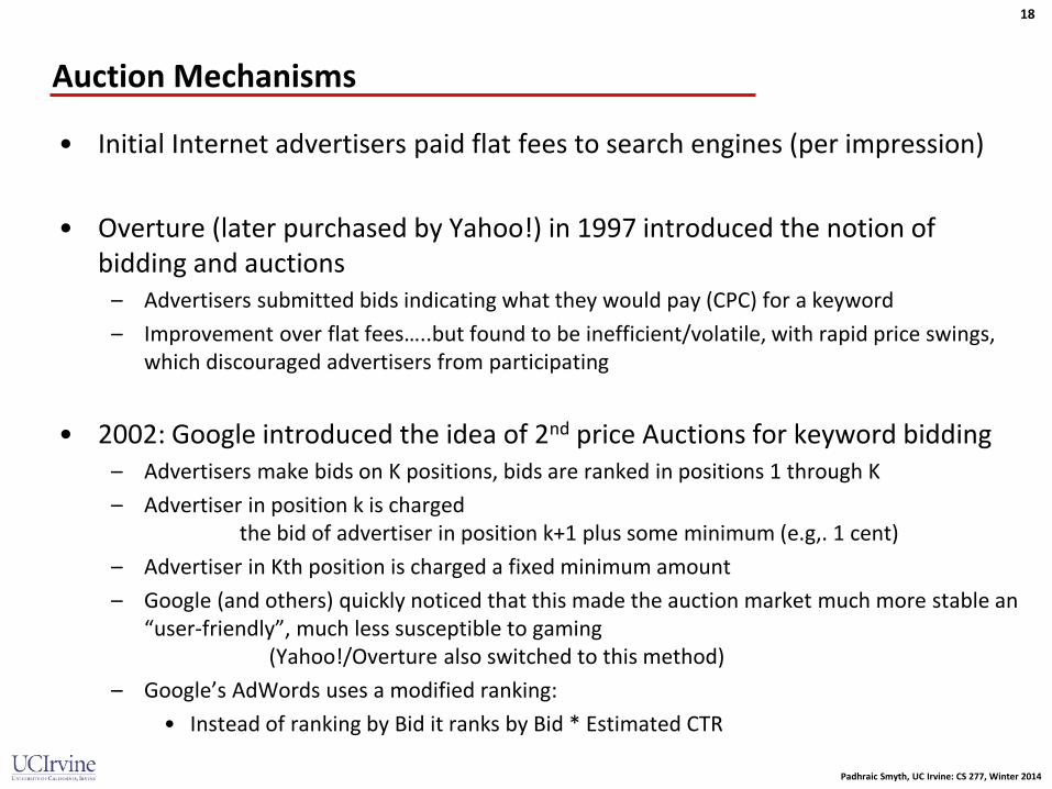
Auction Mechanisms
• Initial Internet advertisers paid flat fees to search engines (per impression)
• Overture (later purchased by Yahoo!) in 1997 introduced the notion of bidding and auctions
– Advertisers submitted bids indicating what they would pay (CPC) for a keyword – Improvement over flat fees…..but found to be inefficient/volatile, with rapid price swings,
which discouraged advertisers from participating
• 2002: Google introduced the idea of 2nd price Auctions for keyword bidding – Advertisers make bids on K positions, bids are ranked in positions 1 through K – Advertiser in position k is charged
the bid of advertiser in position k+1 plus some minimum (e.g,. 1 cent) – Advertiser in Kth position is charged a fixed minimum amount – Google (and others) quickly noticed that this made the auction market much more stable an
“user-friendly”, much less susceptible to gaming (Yahoo!/Overture also switched to this method)
– Google’s AdWords uses a modified ranking: • Instead of ranking by Bid it ranks by Bid * Estimated CTR
Padhraic Smyth, UC Irvine: CS 277, Winter 2014
19
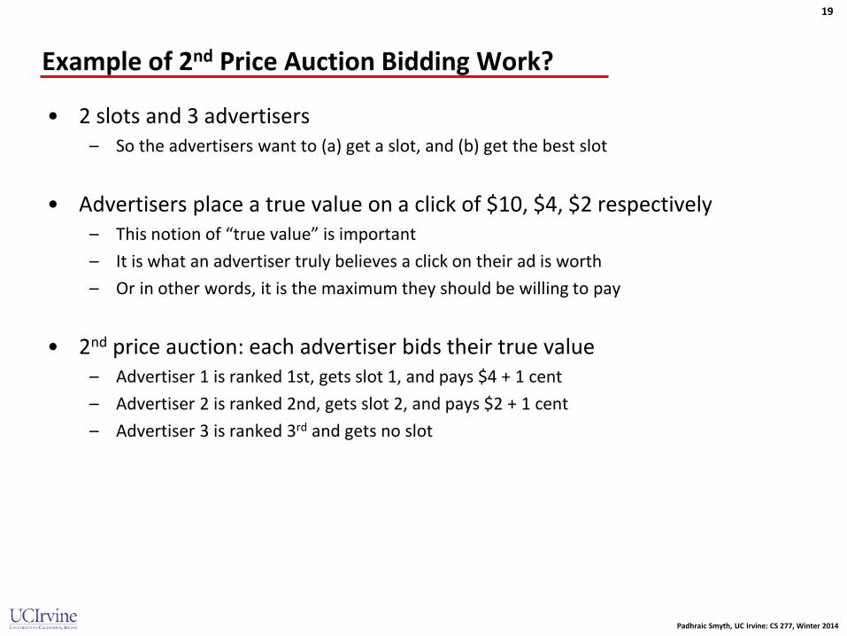
Example of 2nd Price Auction Bidding Work?
• 2 slots and 3 advertisers – So the advertisers want to (a) get a slot, and (b) get the best slot
• Advertisers place a true value on a click of $10, $4, $2 respectively – This notion of “true value” is important – It is what an advertiser truly believes a click on their ad is worth – Or in other words, it is the maximum they should be willing to pay
• 2nd price auction: each advertiser bids their true value – Advertiser 1 is ranked 1st, gets slot 1, and pays $4 + 1 cent – Advertiser 2 is ranked 2nd, gets slot 2, and pays $2 + 1 cent – Advertiser 3 is ranked 3rd and gets no slot

Padhraic Smyth, UC Irvine: CS 277, Winter 2014
20
2nd Price Auctions
• Various economic arguments as to why this is much more efficient than 1st price auctions
– Advertisers have no incentive to bid anything other than their true value – This discourages advertisers from dynamically changing bids, which was a cause of major
instability in earlier first-price auctions
• Methods seems to work particularly well for internet advertising
• References: – Edelman, Ostrovsky, and Schwarz, American Economic Review, 2007 – H. Varian, Online Advertising Markets, American Economic Review, 2010

Padhraic Smyth, UC Irvine: CS 277, Winter 2014
21
Slide from Heinrich Schutze, Introduction to Information Retrieval Class Slides, University of Munich, 2013
Note that the rank here is based on Bid * CTR

Padhraic Smyth, UC Irvine: CS 277, Winter 2014
22
Slide from Heinrich Schutze, Introduction to Information Retrieval Class Slides, University of Munich, 2013
Padhraic Smyth, UC Irvine: CS 277, Winter 2014
23
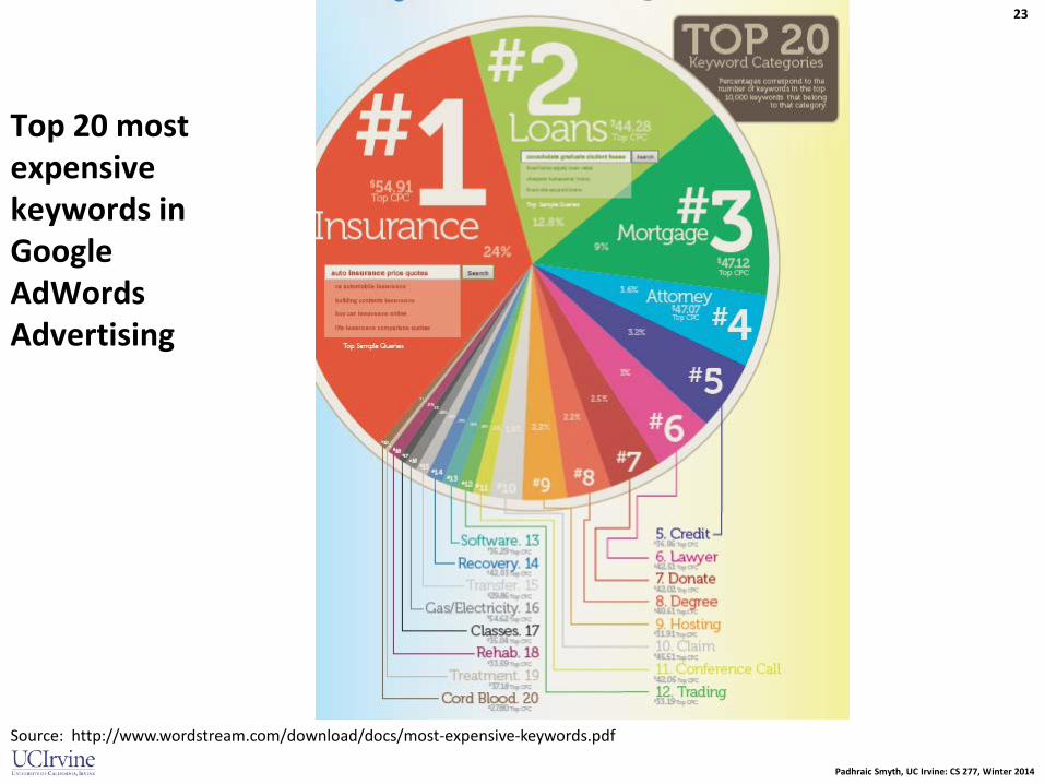
Top 20 most expensive keywords in Google AdWords Advertising
Source: http://www.wordstream.com/download/docs/most-expensive-keywords.pdf

Padhraic Smyth, UC Irvine: CS 277, Winter 2014
24
Metric 2010 2011 2012 2013 Cost per click (CPC) $1.24 $1.04 $0.84 $0.92
Click through rate (CTR) 0.7% 0.4% 0.5% 0.5%
Average Ad Position 3.7 3.0 2.6 2.1
Conversion rate 6.8% 5.3% 3.4% 8.8%
Cost per conversion $13.14 $19.74 $24.40 $10.44
Invalid click rate 6.7% 10.9% 8.0% 8.3%
Examples of Costs per Click
From: survey data from 51 advertisers, at http://www.hochmanconsultants.com/articles/je-hochman-benchmark.shtml
Padhraic Smyth, UC Irvine: CS 277, Winter 2014
25
Predicting Click-Through Rates for Online Advertisements
Padhraic Smyth, UC Irvine: CS 277, Winter 2014
26
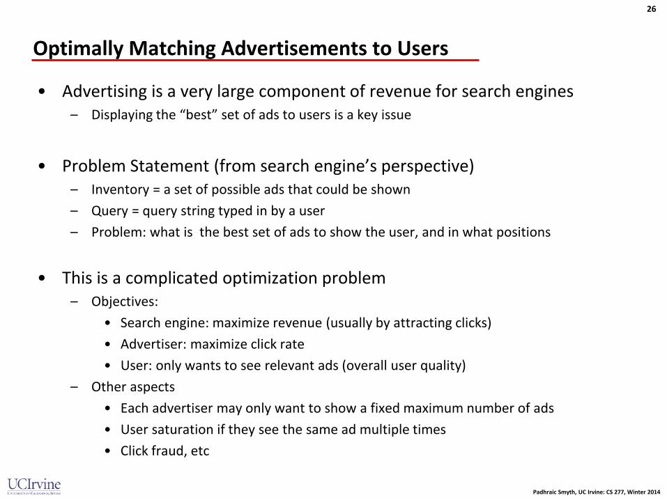
Optimally Matching Advertisements to Users
• Advertising is a very large component of revenue for search engines – Displaying the “best” set of ads to users is a key issue
• Problem Statement (from search engine’s perspective)
– Inventory = a set of possible ads that could be shown – Query = query string typed in by a user – Problem: what is the best set of ads to show the user, and in what positions
• This is a complicated optimization problem – Objectives:
• Search engine: maximize revenue (usually by attracting clicks) • Advertiser: maximize click rate • User: only wants to see relevant ads (overall user quality)
– Other aspects • Each advertiser may only want to show a fixed maximum number of ads • User saturation if they see the same ad multiple times • Click fraud, etc

Padhraic Smyth, UC Irvine: CS 277, Winter 2014
27
Cost-Per-Click (CPC) Model
• Cost-Per-Click, or CPC: – Search engine is paid every time an ad is clicked by a user
• Simple Expected Revenue Model E[ revenue ] = p(click | ad) CPC ad
• Simple heuristic
– Order the ads in terms of expected revenue

Padhraic Smyth, UC Irvine: CS 277, Winter 2014
28
Metric 2010 2011 2012 2013 Cost per click (CPC) $1.24 $1.04 $0.84 $0.92
Click through rate (CTR) 0.7% 0.4% 0.5% 0.5%
Average Ad Position 3.7 3.0 2.6 2.1
Conversion rate 6.8% 5.3% 3.4% 8.8%
Cost per conversion $13.14 $19.74 $24.40 $10.44
Invalid click rate 6.7% 10.9% 8.0% 8.3%
Examples of Costs per Click
From: survey data from 51 advertisers, at http://www.hochmanconsultants.com/articles/je-hochman-benchmark.shtml
Padhraic Smyth, UC Irvine: CS 277, Winter 2014
29
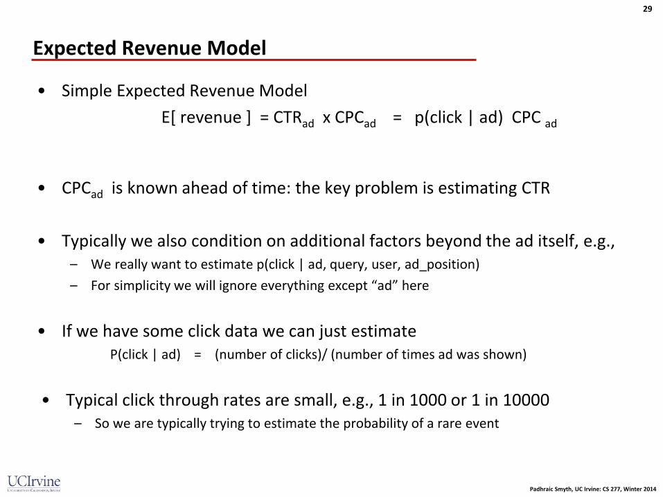
Expected Revenue Model
• Simple Expected Revenue Model E[ revenue ] = CTRad x CPCad = p(click | ad) CPC ad
• CPCad is known ahead of time: the key problem is estimating CTR • Typically we also condition on additional factors beyond the ad itself, e.g.,
– We really want to estimate p(click | ad, query, user, ad_position) – For simplicity we will ignore everything except “ad” here
• If we have some click data we can just estimate P(click | ad) = (number of clicks)/ (number of times ad was shown)
• Typical click through rates are small, e.g., 1 in 1000 or 1 in 10000 – So we are typically trying to estimate the probability of a rare event
Padhraic Smyth, UC Irvine: CS 277, Winter 2014
30
Computing the CTR from Click Data
• Estimate of CTR = (number of clicks)/(number of views)
• Number of clicks = number of times ad was clicked
• Number of views? – Use a “discount” model based on eye-tracking to estimate how many times the ad was seen
by users – So number of views is total number of times ad was shown, “discounted” by position model
Padhraic Smyth, UC Irvine: CS 277, Winter 2014
31
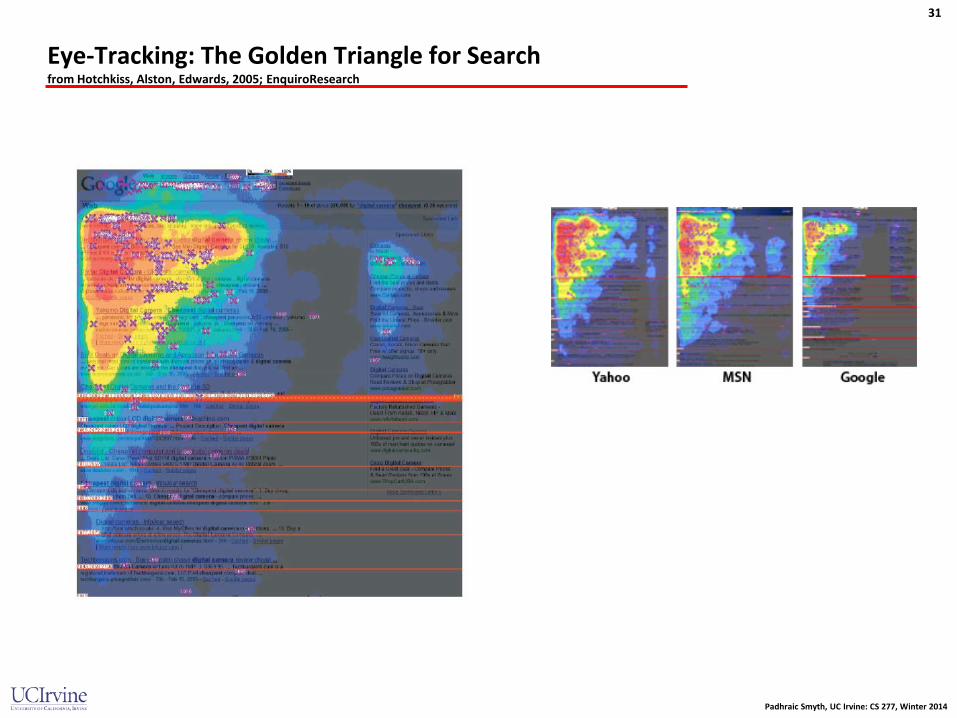
Eye-Tracking: The Golden Triangle for Search from Hotchkiss, Alston, Edwards, 2005; EnquiroResearch

Padhraic Smyth, UC Irvine: CS 277, Winter 2014
32
Simple Example of CTR Estimation
• Assume that the true P(click | ad) = 10-4
– Say we have seen r clicks, from N showings of the ad – Our estimate of P(click | ad) = P’ = r/N
• What is our uncertainty about P’? Simple binomial model, assume N p > 5, i.e., N > 5 x 10⁴ in our problem -> 95% confidence interval is
𝑤 = 1.96 𝑝 (1 − 𝑝) 𝑁⁄ ≈ 0.02 𝑁⁄ Say we want w < 10-5 (10% of the true value)
Rearranging terms above this means we need
𝑁 > 0.02 105 or N > 4 x 10 6
This means we need a very large N to be confident in our estimation of small probabilities

Padhraic Smyth, UC Irvine: CS 277, Winter 2014
33
Difficulty of CTR Prediction Problem
• Clickthrough rates are small -> need large number of impressions to get reliable estimates
• Every day there will be a large number of new ads that the ad placement algorithm has not seen before, i.e., with unknown CTR
• Making mistakes is expensive – Say we show ad A 10 million times, and the CPC is $1 with a true CTR of 10-4
– And we don’t show ad B, which has a CPC of $1 with a true CTR of 10-2
– Then the “cost of learning” about ad A (versus not showing B) is 10-2 times 10 million, or $100,000 (!)

Padhraic Smyth, UC Irvine: CS 277, Winter 2014
55
Online Learning of ClickThrough Rates
Padhraic Smyth, UC Irvine: CS 277, Winter 2014
56
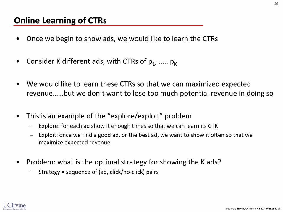
Online Learning of CTRs
• Once we begin to show ads, we would like to learn the CTRs
• Consider K different ads, with CTRs of p1, ….. pK
• We would like to learn these CTRs so that we can maximized expected revenue……but we don’t want to lose too much potential revenue in doing so
• This is an example of the “explore/exploit” problem – Explore: for each ad show it enough times so that we can learn its CTR – Exploit: once we find a good ad, or the best ad, we want to show it often so that we
maximize expected revenue
• Problem: what is the optimal strategy for showing the K ads? – Strategy = sequence of (ad, click/no-click) pairs
Padhraic Smyth, UC Irvine: CS 277, Winter 2014
57
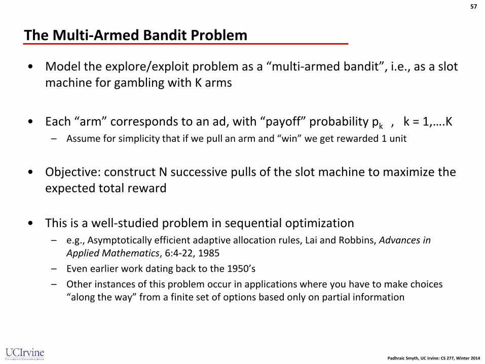
The Multi-Armed Bandit Problem
• Model the explore/exploit problem as a “multi-armed bandit”, i.e., as a slot machine for gambling with K arms
• Each “arm” corresponds to an ad, with “payoff” probability pk , k = 1,….K – Assume for simplicity that if we pull an arm and “win” we get rewarded 1 unit
• Objective: construct N successive pulls of the slot machine to maximize the expected total reward
• This is a well-studied problem in sequential optimization – e.g., Asymptotically efficient adaptive allocation rules, Lai and Robbins, Advances in
Applied Mathematics, 6:4-22, 1985 – Even earlier work dating back to the 1950’s – Other instances of this problem occur in applications where you have to make choices
“along the way” from a finite set of options based only on partial information

Padhraic Smyth, UC Irvine: CS 277, Winter 2014
58
Theoretical Framework
• K bandits, with payoff probabilities pk , k = 1,….K, and unit rewards = 1 – Assume for simplicity that pk probabilities and rewards don’t change over time – Also assume that bandits are memoryless (as in coin-tossing)
• Let Xk be the reward on any trial for bandit k. Assume for simplicity that Xk =1 with probability pk, and = 0 with probability 1 - pk Expected reward from bandit k is E [Xk] = 1 pk + 0 (1- pk) = pk
• Optimal strategy to maximize the expected reward?
– Always select the k value that maximizes E [Xk] , i.e., the largest probability pk – This optimal strategy exists only in theory, if we know the pk ‘s (which we don’t)
• Various theoretical analyses look at what happens on average by using certain types of strategies.
Expected Regret(S) = E [reward |optimal strategy] – E [reward | strategy S]

Padhraic Smyth, UC Irvine: CS 277, Winter 2014
59
Naïve Strategies
• Deterministic Greedy Strategy: – at iteration N, pick the bandit that has performed best up to this time – Weakness?
• Will under-explore bandits and may easily select a sub-optimal bandit forever
• Play-the-Winner Strategy – At iteration N
• play the bandit from iteration N-1 if it was successful, otherwise • select another arm uniformly at random or cycle through them deterministically
– This is the optimal thing to do if the bandit was successful at time N-1 – But not necessarily optimal to switch away from this bandit if it failed – Thus, this strategy tends to switch too much and over-explores
(see Berry and Fristedt, Bandit Problems: Sequential Allocation of Experiments, Chapman & Hall, 1985)
Note that both strategies above perform even more poorly if the learning is happening in batch mode rather than at each iteration.
Padhraic Smyth, UC Irvine: CS 277, Winter 2014
60
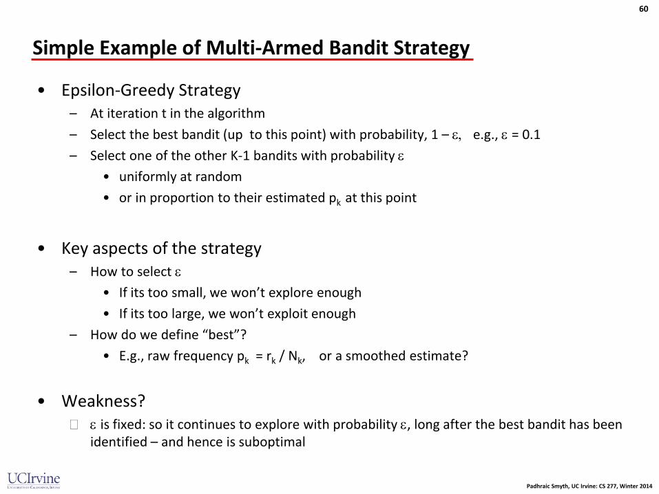
Simple Example of Multi-Armed Bandit Strategy
• Epsilon-Greedy Strategy – At iteration t in the algorithm – Select the best bandit (up to this point) with probability, 1 – ε, e.g., ε = 0.1 – Select one of the other K-1 bandits with probability ε
• uniformly at random • or in proportion to their estimated pk at this point
• Key aspects of the strategy
– How to select ε • If its too small, we won’t explore enough • If its too large, we won’t exploit enough
– How do we define “best”? • E.g., raw frequency pk = rk / Nk, or a smoothed estimate?
• Weakness? � ε is fixed: so it continues to explore with probability ε, long after the best bandit has been
identified – and hence is suboptimal

Padhraic Smyth, UC Irvine: CS 277, Winter 2014
61
Other Examples of Strategies
• Epsilon-greedy where we decrease ε as the experiment progress – Makes intuitive sense: explore a lot at first, then start to exploit more – Adds an additional “tuning” parameter of how to decrease ε
• Epsilon-first Strategy
– Pure exploration followed by pure exploitation – First explore for εN trials, selecting bandits uniformly at random – Then exploit for (1-ε)N trials, selecting the best bandit from the explore phase
• Theoretical analyses provide results like bounds on the rates at which arms should be played, as a function of the true (unknown) pk values
– These results provide very useful insights and general guidance – But don’t provide specific strategies
Padhraic Smyth, UC Irvine: CS 277, Winter 2014
62
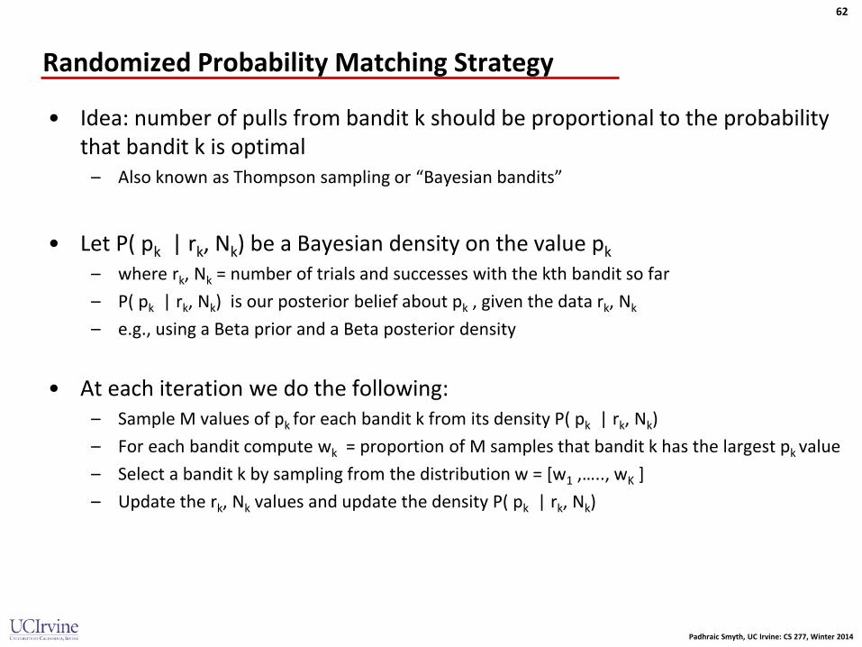
Randomized Probability Matching Strategy
• Idea: number of pulls from bandit k should be proportional to the probability that bandit k is optimal
– Also known as Thompson sampling or “Bayesian bandits”
• Let P( pk | rk, Nk) be a Bayesian density on the value pk
– where rk, Nk = number of trials and successes with the kth bandit so far – P( pk | rk, Nk) is our posterior belief about pk , given the data rk, Nk
– e.g., using a Beta prior and a Beta posterior density
• At each iteration we do the following: – Sample M values of pk for each bandit k from its density P( pk | rk, Nk) – For each bandit compute wk = proportion of M samples that bandit k has the largest pk value – Select a bandit k by sampling from the distribution w = [w1 ,….., wK ] – Update the rk, Nk values and update the density P( pk | rk, Nk)
Padhraic Smyth, UC Irvine: CS 277, Winter 2014
63
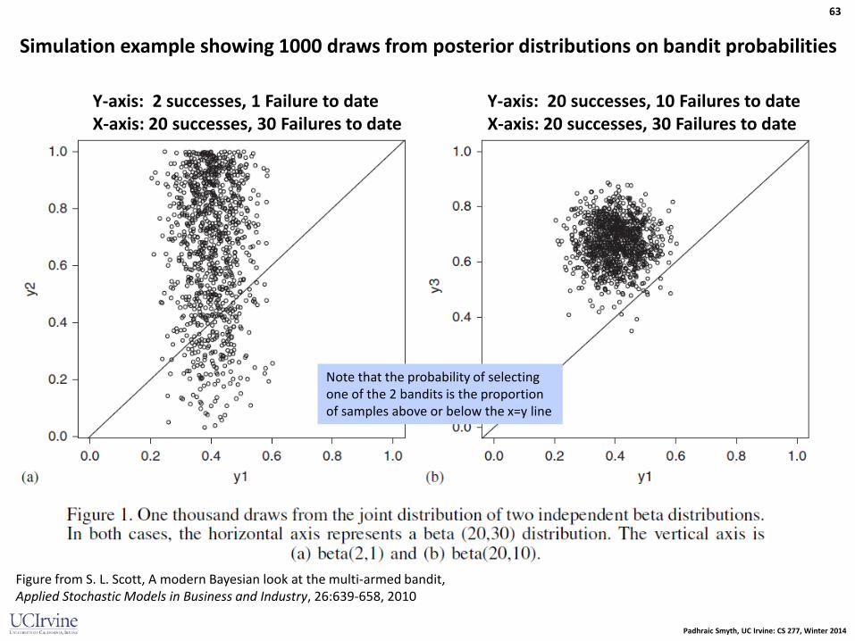
Simulation example showing 1000 draws from posterior distributions on bandit probabilities
Y-axis: 2 successes, 1 Failure to date X-axis: 20 successes, 30 Failures to date
Y-axis: 20 successes, 10 Failures to date X-axis: 20 successes, 30 Failures to date
Figure from S. L. Scott, A modern Bayesian look at the multi-armed bandit, Applied Stochastic Models in Business and Industry, 26:639-658, 2010
Note that the probability of selecting one of the 2 bandits is the proportion of samples above or below the x=y line
Padhraic Smyth, UC Irvine: CS 277, Winter 2014
64
Randomized Probability Matching Strategy
• Strengths – Works well on a wide-range of problems – Relatively simple to implement – Relatively free of tuning parameters – Flexible enough to accommodate more complicated versions of the problem – Balances exploration and exploitation in an intuitive way
• Weaknesses – Requires more computation to select an arm at each iteration – Theoretical results/guarantees, relative to other methods, not generally known (yet)
For additional discussion and experiments see S. L. Scott, A modern Bayesian look at the multi-armed bandit, Applied Stochastic Models in Business and Industry, 26:639-658, 2010
Padhraic Smyth, UC Irvine: CS 277, Winter 2014
65
Click Fraud
• Click fraud = generation of artificial (non-human) clicks for ads
• Why? – Artificially increases the costs for the advertiser (for CPC) – Artificially increases the revenue of the site hosting the ad (for CPC)
• Click Quality Teams – All major search engines have full-time teams monitoring/managing click fraud – Use a combination of human analysis and machine learning algorithms
• Controversial topic – Advertisers say search engines are not doing enough, claim fraud clicks are > 20% – Search engines reluctant to publish too much data on frauds, claim fraud click percentage is
much lpower
Mining of Massive Datasets
Jure Leskovec, Anand Rajaraman, Jeff Ullman Stanford University
http://www.mmds.org
Note to other teachers and users of these slides: We would be delighted if you found this our
material useful in giving your own lectures. Feel free to use these slides verbatim, or to modify
them to fit your own needs. If you make use of a significant portion of these slides in your own
lecture, please include this message, or a link to our web site: http://www.mmds.org

� Classic model of algorithms
� You get to see the entire input, then compute
some function of it
� In this context, “offline algorithm”
� Online Algorithms
� You get to see the input one piece at a time, and
need to make irrevocable decisions along the way
� Similar to the data stream model
2J. Leskovec, A. Rajaraman, J. Ullman: Mining of Massive Datasets, http://www.mmds.org

1
2
3
4
a
b
c
dBoys Girls
4J. Leskovec, A. Rajaraman, J. Ullman: Mining of Massive Datasets, http://www.mmds.org
Nodes: Boys and Girls; Edges: Preferences
Goal: Match boys to girls so that maximum
number of preferences is satisfied
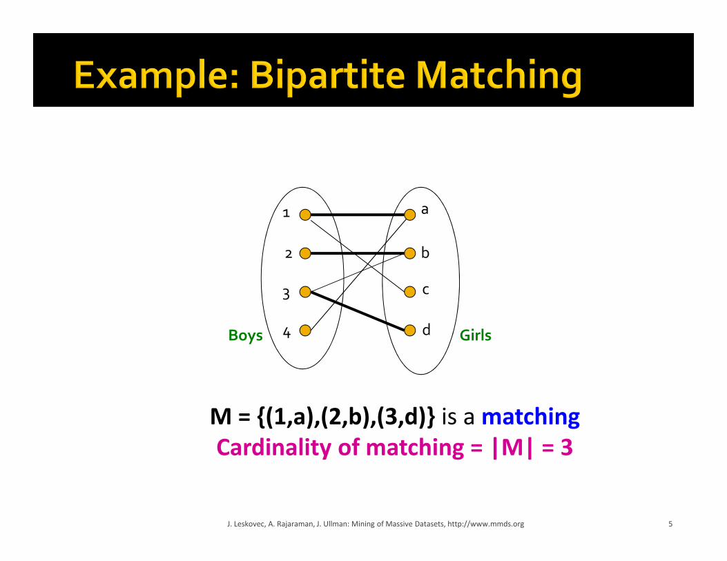
M = {(1,a),(2,b),(3,d)} is a matching
Cardinality of matching = |M| = 3
1
2
3
4
a
b
c
dBoys Girls
5J. Leskovec, A. Rajaraman, J. Ullman: Mining of Massive Datasets, http://www.mmds.org

1
2
3
4
a
b
c
dBoys Girls
M = {(1,c),(2,b),(3,d),(4,a)} is a
perfect matching
6J. Leskovec, A. Rajaraman, J. Ullman: Mining of Massive Datasets, http://www.mmds.org
Perfect matching … all vertices of the graph are matched
Maximum matching … a matching that contains the largest possible number of matches
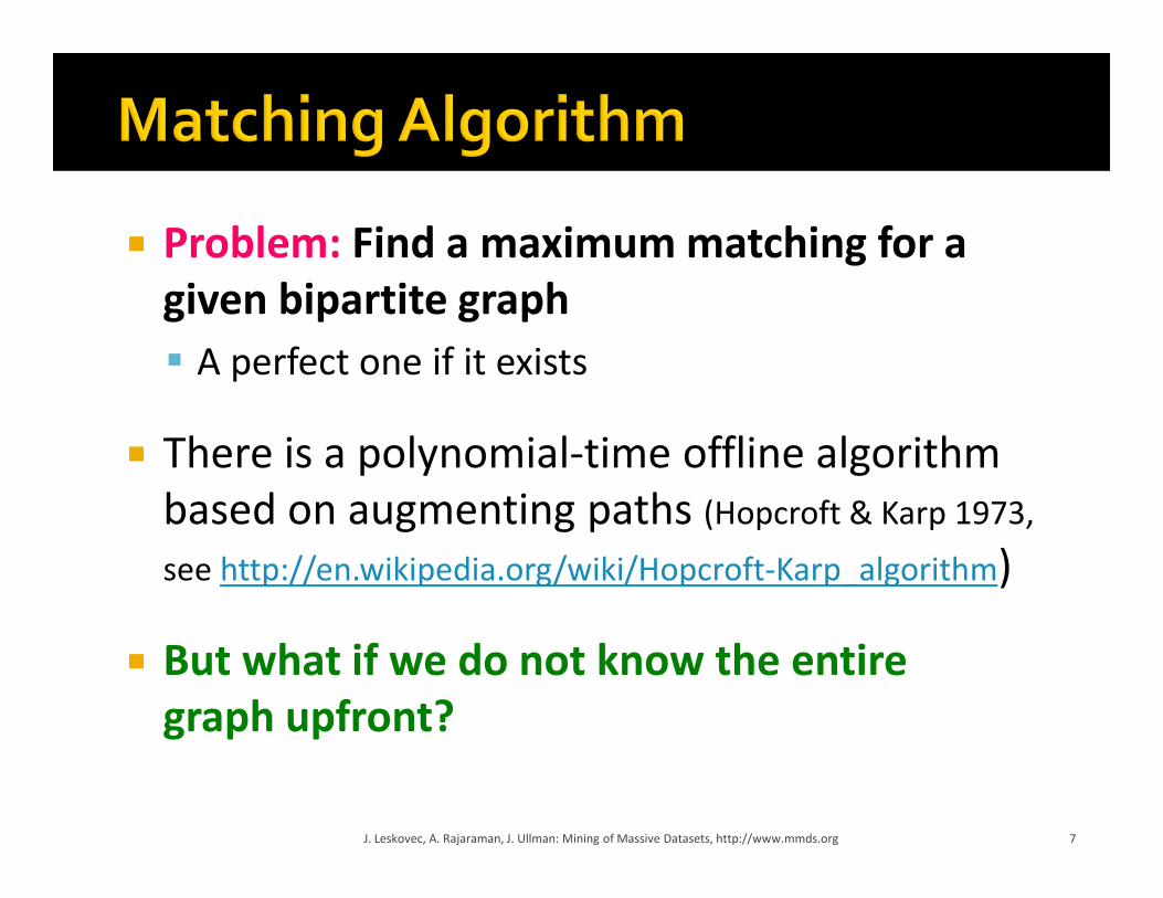
� Problem: Find a maximum matching for a
given bipartite graph
� A perfect one if it exists
� There is a polynomial-time offline algorithm
based on augmenting paths (Hopcroft & Karp 1973,
see http://en.wikipedia.org/wiki/Hopcroft-Karp_algorithm)
� But what if we do not know the entire
graph upfront?
7J. Leskovec, A. Rajaraman, J. Ullman: Mining of Massive Datasets, http://www.mmds.org
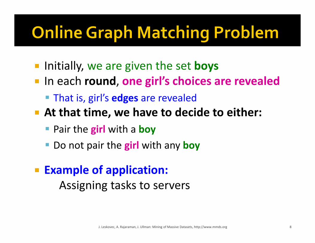
� Initially, we are given the set boys
� In each round, one girl’s choices are revealed
� That is, girl’s edges are revealed
� At that time, we have to decide to either:
� Pair the girl with a boy
� Do not pair the girl with any boy
� Example of application:
Assigning tasks to servers
8J. Leskovec, A. Rajaraman, J. Ullman: Mining of Massive Datasets, http://www.mmds.org

J. Leskovec, A. Rajaraman, J. Ullman: Mining of Massive Datasets, http://www.mmds.org 9
1
2
3
4
a
b
c
d
(1,a)(2,b)
(3,d)
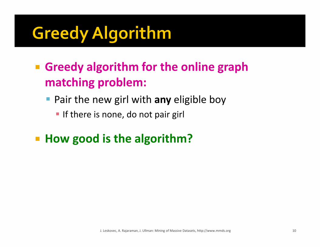
� Greedy algorithm for the online graph
matching problem:
� Pair the new girl with any eligible boy
� If there is none, do not pair girl
� How good is the algorithm?
10J. Leskovec, A. Rajaraman, J. Ullman: Mining of Massive Datasets, http://www.mmds.org

� For input I, suppose greedy produces
matching Mgreedy while an optimal
matching is Mopt
Competitive ratio =
minall possible inputs I (|Mgreedy|/|Mopt|)
(what is greedy’s worst performance over all possible inputs I)
11J. Leskovec, A. Rajaraman, J. Ullman: Mining of Massive Datasets, http://www.mmds.org

� Consider a case: Mgreedy≠ Mopt
� Consider the set G of girls
matched in Mopt but not in Mgreedy
� Then every boy B adjacent to girls
in G is already matched in Mgreedy:
� If there would exist such non-matched
(by Mgreedy) boy adjacent to a non-matched
girl then greedy would have matched them
� Since boys B are already matched in Mgreedy then
(1) |Mgreedy|≥ |B|
J. Leskovec, A. Rajaraman, J. Ullman: Mining of Massive Datasets, http://www.mmds.org 12
a
b
c
d
G={ }B={ }
Mopt1
2
3
4
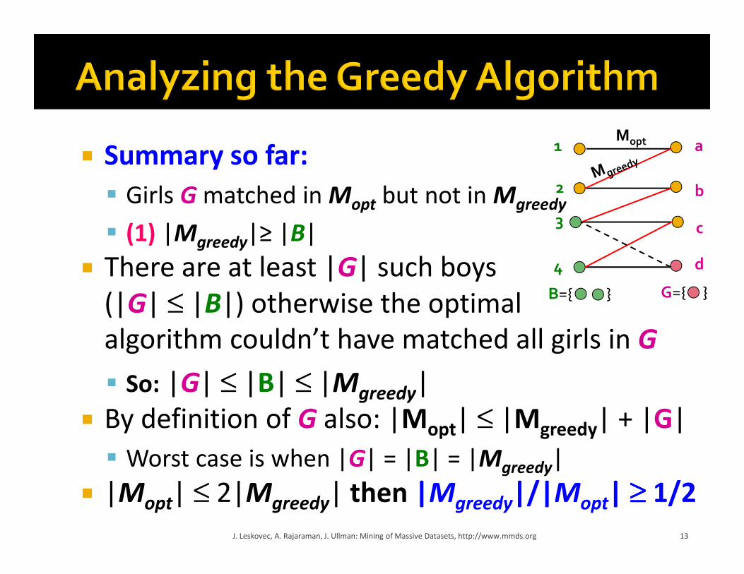
� Summary so far:
� Girls G matched in Mopt but not in Mgreedy
� (1) |Mgreedy|≥ |B|
� There are at least |G| such boys
(|G| ≤ |B|) otherwise the optimal
algorithm couldn’t have matched all girls in G
� So: |G| ≤ |B| ≤ |Mgreedy|
� By definition of G also: |Mopt| ≤ |Mgreedy| + |G|
� Worst case is when |G| = |B| = |Mgreedy|
� |Mopt| ≤ 2|Mgreedy| then |Mgreedy|/|Mopt| ≥≥≥≥ 1/2
J. Leskovec, A. Rajaraman, J. Ullman: Mining of Massive Datasets, http://www.mmds.org 13
a
b
c
d
G={ }B={ }
Mopt1
2
3
4

1
2
3
4
a
b
c
(1,a)(2,b)
d
14J. Leskovec, A. Rajaraman, J. Ullman: Mining of Massive Datasets, http://www.mmds.org

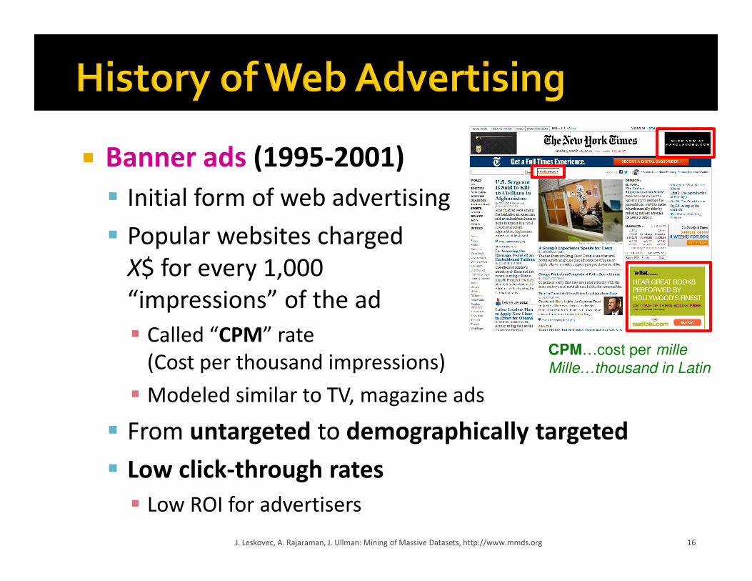
� Banner ads (1995-2001)
� Initial form of web advertising
� Popular websites charged
X$ for every 1,000
“impressions” of the ad
� Called “CPM” rate
(Cost per thousand impressions)
� Modeled similar to TV, magazine ads
� From untargeted to demographically targeted
� Low click-through rates
� Low ROI for advertisers
J. Leskovec, A. Rajaraman, J. Ullman: Mining of Massive Datasets, http://www.mmds.org 16
CPM…cost per mille
Mille…thousand in Latin

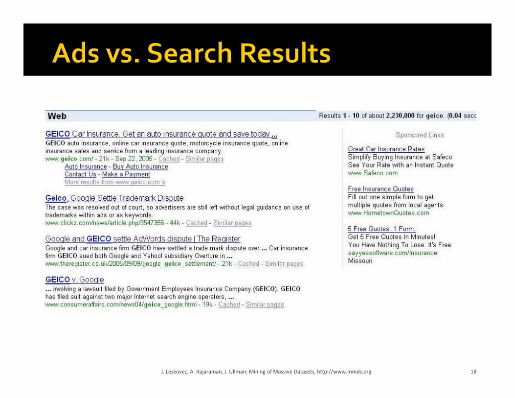
� Introduced by Overture around 2000
� Advertisers bid on search keywords
� When someone searches for that keyword, the
highest bidder’s ad is shown
� Advertiser is charged only if the ad is clicked on
� Similar model adopted by Google with some
changes around 2002
� Called Adwords
17J. Leskovec, A. Rajaraman, J. Ullman: Mining of Massive Datasets, http://www.mmds.org
18J. Leskovec, A. Rajaraman, J. Ullman: Mining of Massive Datasets, http://www.mmds.org
� Performance-based advertising works!
� Multi-billion-dollar industry
� Interesting problem:
What ads to show for a given query?
� (Today’s lecture)
� If I am an advertiser, which search terms
should I bid on and how much should I bid?
� (Not focus of today’s lecture)
19J. Leskovec, A. Rajaraman, J. Ullman: Mining of Massive Datasets, http://www.mmds.org
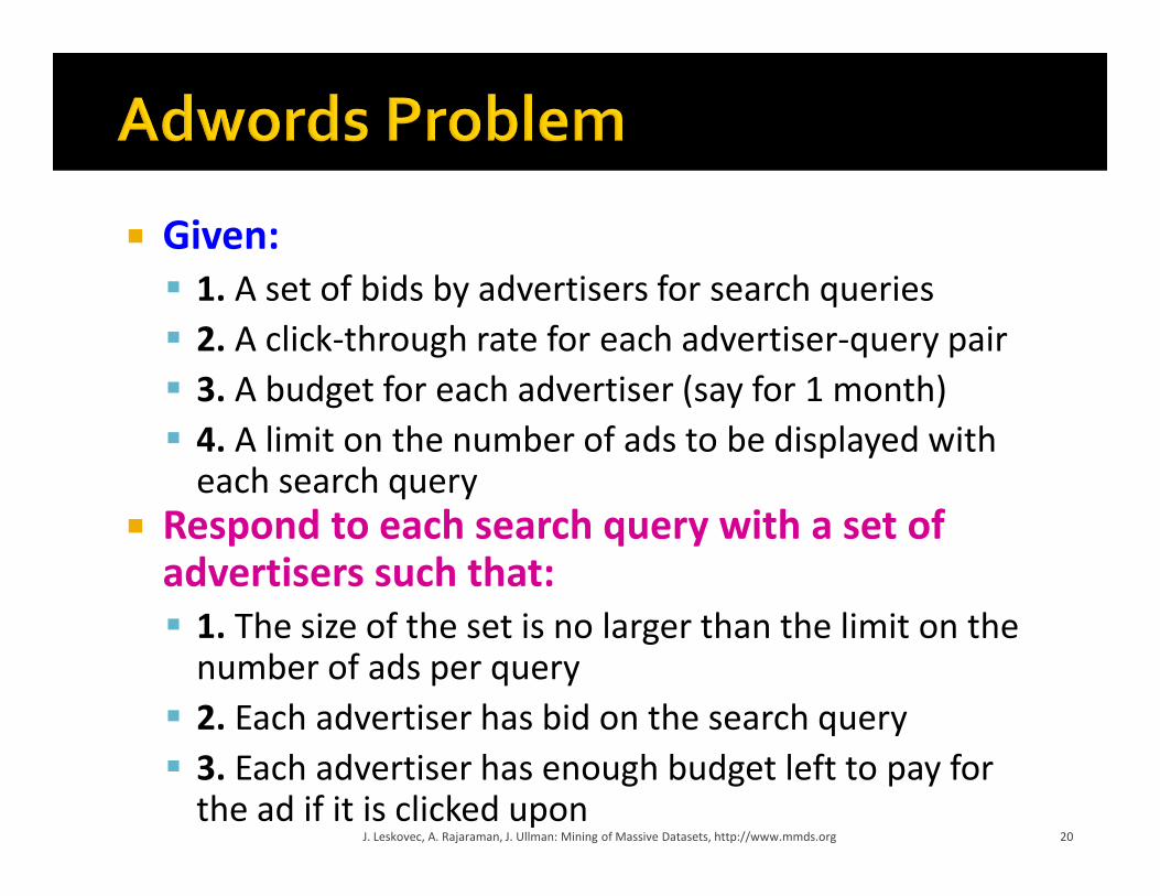
� Given:
� 1. A set of bids by advertisers for search queries
� 2. A click-through rate for each advertiser-query pair
� 3. A budget for each advertiser (say for 1 month)
� 4. A limit on the number of ads to be displayed with each search query
� Respond to each search query with a set of advertisers such that:
� 1. The size of the set is no larger than the limit on the number of ads per query
� 2. Each advertiser has bid on the search query
� 3. Each advertiser has enough budget left to pay for the ad if it is clicked upon
J. Leskovec, A. Rajaraman, J. Ullman: Mining of Massive Datasets, http://www.mmds.org 20
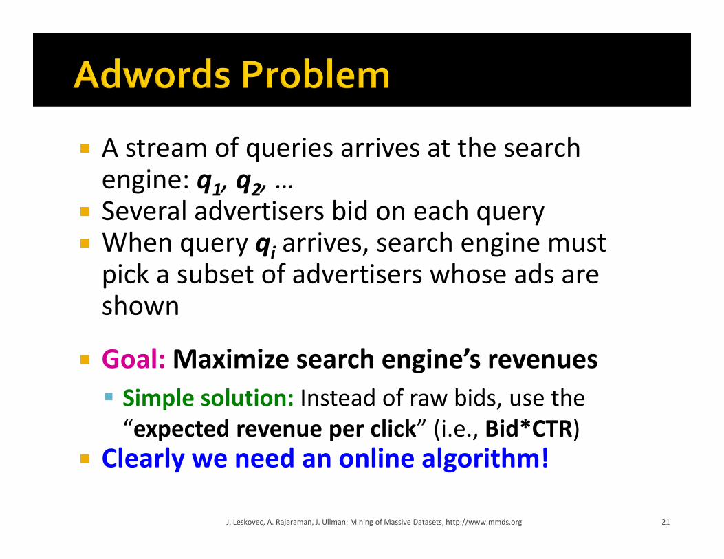
� A stream of queries arrives at the search engine: q1, q2, …
� Several advertisers bid on each query� When query qi arrives, search engine must
pick a subset of advertisers whose ads are shown
� Goal: Maximize search engine’s revenues
� Simple solution: Instead of raw bids, use the
“expected revenue per click” (i.e., Bid*CTR)
� Clearly we need an online algorithm!
21J. Leskovec, A. Rajaraman, J. Ullman: Mining of Massive Datasets, http://www.mmds.org
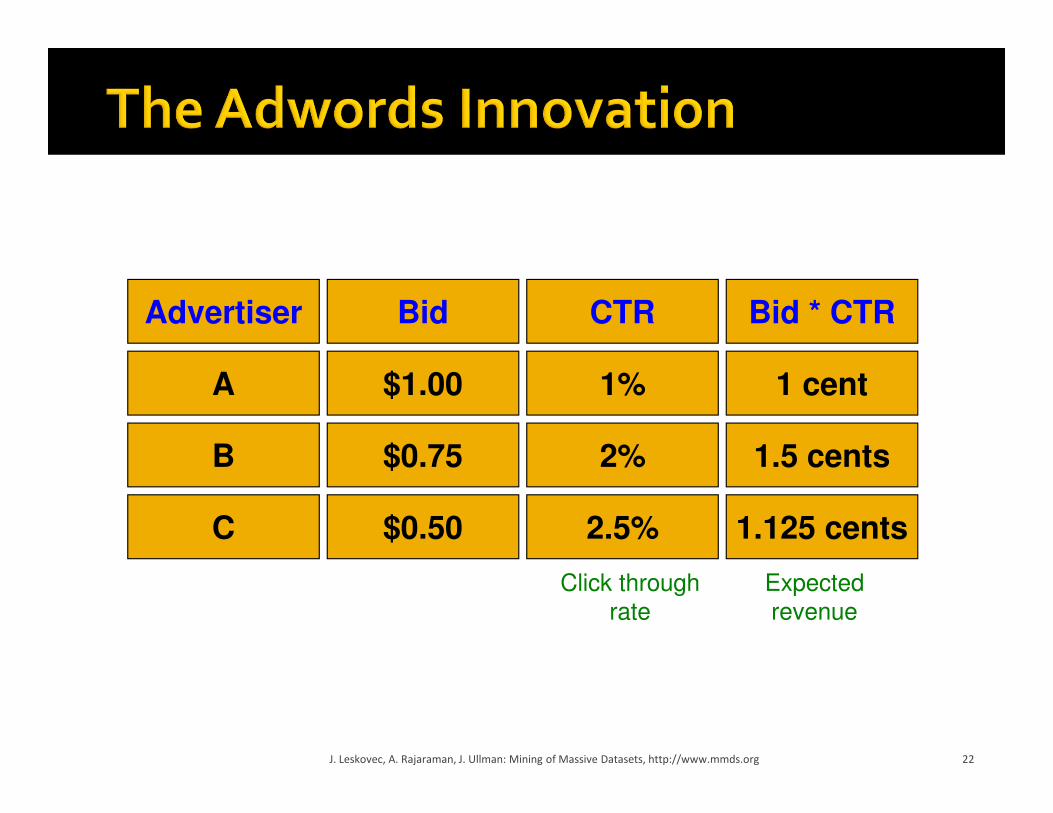
J. Leskovec, A. Rajaraman, J. Ullman: Mining of Massive Datasets, http://www.mmds.org 22
Advertiser Bid CTR Bid * CTR
A
B
C
$1.00
$0.75
$0.50
1%
2%
2.5%
1 cent
1.5 cents
1.125 cents
Click through
rate
Expected
revenue
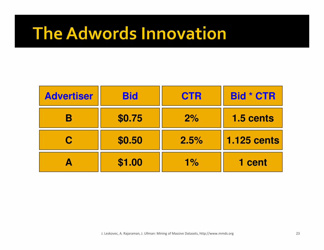
J. Leskovec, A. Rajaraman, J. Ullman: Mining of Massive Datasets, http://www.mmds.org 23
Advertiser Bid CTR Bid * CTR
A
B
C
$1.00
$0.75
$0.50
1%
2%
2.5%
1 cent
1.5 cents
1.125 cents

� Two complications:
� Budget
� CTR of an ad is unknown
� Each advertiser has a limited budget
� Search engine guarantees that the advertiser
will not be charged more than their daily budget
J. Leskovec, A. Rajaraman, J. Ullman: Mining of Massive Datasets, http://www.mmds.org 24
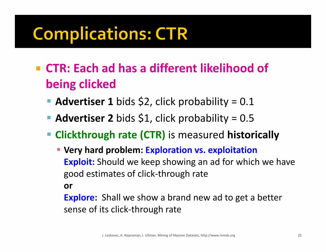
� CTR: Each ad has a different likelihood of
being clicked
� Advertiser 1 bids $2, click probability = 0.1
� Advertiser 2 bids $1, click probability = 0.5
� Clickthrough rate (CTR) is measured historically
� Very hard problem: Exploration vs. exploitation
Exploit: Should we keep showing an ad for which we have
good estimates of click-through rate
or
Explore: Shall we show a brand new ad to get a better
sense of its click-through rate
J. Leskovec, A. Rajaraman, J. Ullman: Mining of Massive Datasets, http://www.mmds.org 25

� Our setting: Simplified environment
� There is 1 ad shown for each query
� All advertisers have the same budget B
� All ads are equally likely to be clicked
� Value of each ad is the same (=1)
� Simplest algorithm is greedy:
� For a query pick any advertiser who has
bid 1 for that query
� Competitive ratio of greedy is 1/2
26J. Leskovec, A. Rajaraman, J. Ullman: Mining of Massive Datasets, http://www.mmds.org
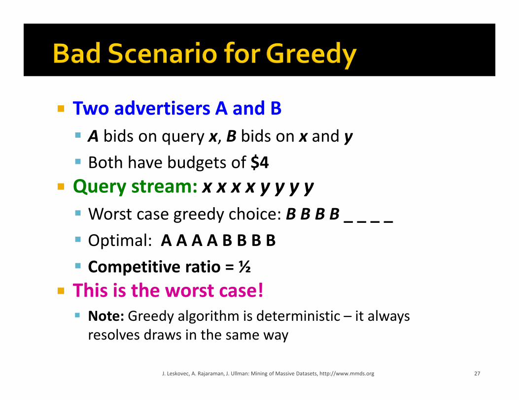
� Two advertisers A and B
� A bids on query x, B bids on x and y
� Both have budgets of $4
� Query stream: x x x x y y y y
� Worst case greedy choice: B B B B _ _ _ _
� Optimal: A A A A B B B B
� Competitive ratio = ½
� This is the worst case!� Note: Greedy algorithm is deterministic – it always
resolves draws in the same way
27J. Leskovec, A. Rajaraman, J. Ullman: Mining of Massive Datasets, http://www.mmds.org

� BALANCE Algorithm by Mehta, Saberi,
Vazirani, and Vazirani
� For each query, pick the advertiser with the
largest unspent budget
� Break ties arbitrarily (but in a deterministic way)
28J. Leskovec, A. Rajaraman, J. Ullman: Mining of Massive Datasets, http://www.mmds.org

� Two advertisers A and B
� A bids on query x, B bids on x and y
� Both have budgets of $4
� Query stream: x x x x y y y y
� BALANCE choice: A B A B B B _ _
� Optimal: A A A A B B B B
� In general: For BALANCE on 2 advertisers
Competitive ratio = ¾
29J. Leskovec, A. Rajaraman, J. Ullman: Mining of Massive Datasets, http://www.mmds.org
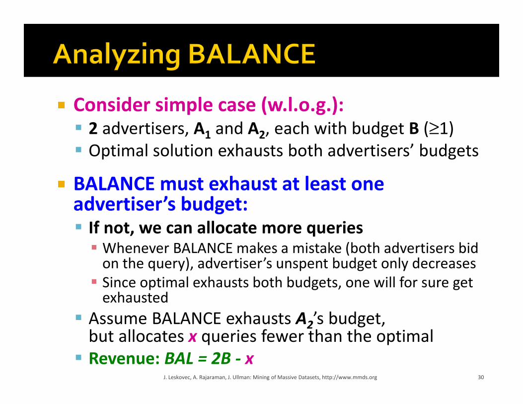
� Consider simple case (w.l.o.g.): � 2 advertisers, A1 and A2, each with budget B (≥1)
� Optimal solution exhausts both advertisers’ budgets
� BALANCE must exhaust at least one advertiser’s budget:� If not, we can allocate more queries
� Whenever BALANCE makes a mistake (both advertisers bid on the query), advertiser’s unspent budget only decreases
� Since optimal exhausts both budgets, one will for sure get exhausted
� Assume BALANCE exhausts A2’s budget, but allocates x queries fewer than the optimal
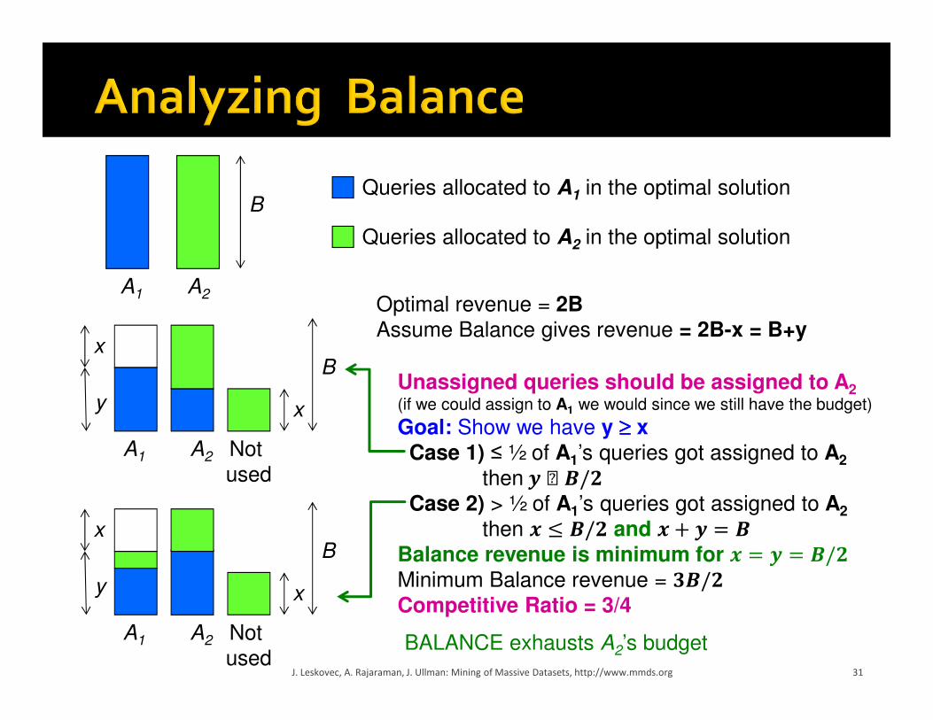
� Revenue: BAL = 2B - xJ. Leskovec, A. Rajaraman, J. Ullman: Mining of Massive Datasets, http://www.mmds.org 30
A1 A2
B
xy
B
A1 A2
x
Optimal revenue = 2BAssume Balance gives revenue = 2B-x = B+y
Unassigned queries should be assigned to A2(if we could assign to A1 we would since we still have the budget)
Goal: Show we have y ≥≥≥≥ xCase 1) ≤ ½ of A1’s queries got assigned to A2
then ���/�
Case 2) > ½ of A1’s queries got assigned to A2
then � � �/� and � � �
Balance revenue is minimum for � � �/�
Minimum Balance revenue = ��/�
Competitive Ratio = 3/4
Queries allocated to A1
in the optimal solution
Queries allocated to A2
in the optimal solution
Not
used
31J. Leskovec, A. Rajaraman, J. Ullman: Mining of Massive Datasets, http://www.mmds.org
BALANCE exhausts A2’s budget
xy
B
A1 A2
x
Not
used

� In the general case, worst competitive ratio
of BALANCE is 1–1/e = approx. 0.63
� Interestingly, no online algorithm has a better
competitive ratio!
� Let’s see the worst case example that gives
this ratio
32J. Leskovec, A. Rajaraman, J. Ullman: Mining of Massive Datasets, http://www.mmds.org
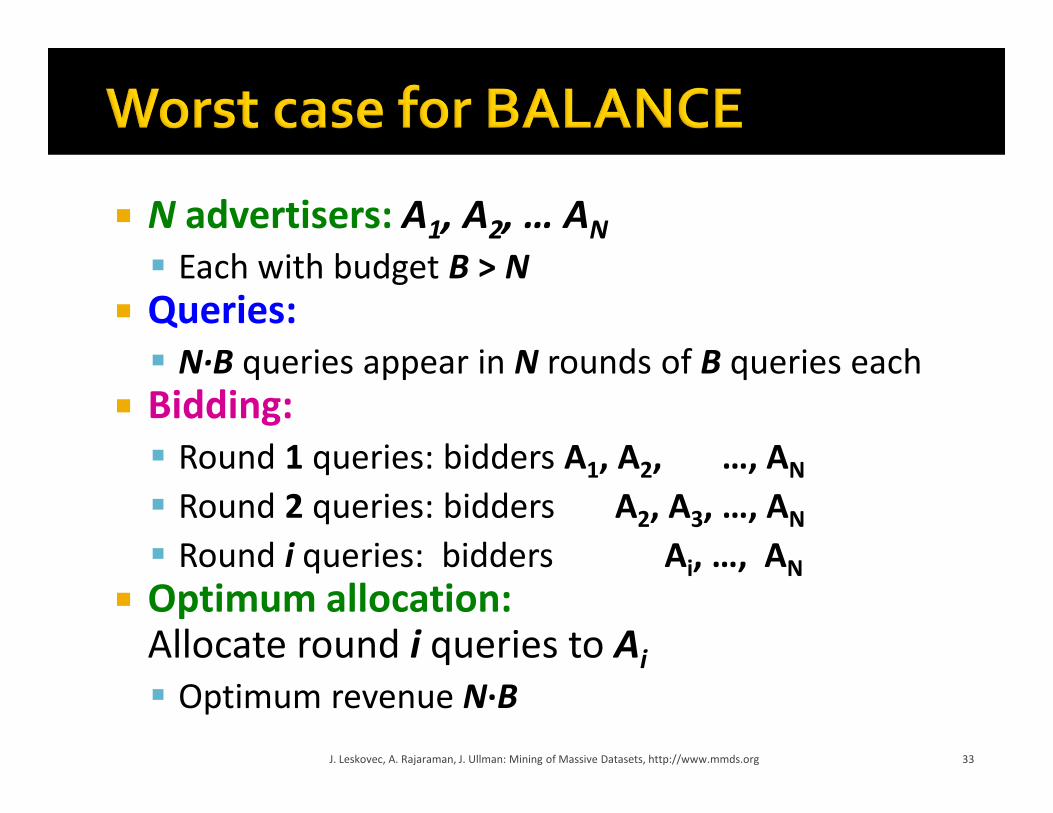
� N advertisers: A1, A2, … AN
� Each with budget B > N
� Queries:
� N∙B queries appear in N rounds of B queries each
� Bidding:
� Round 1 queries: bidders A1, A2, …, AN
� Round 2 queries: bidders A2, A3, …, AN
� Round i queries: bidders Ai, …, AN
� Optimum allocation: Allocate round i queries to Ai
� Optimum revenue N∙B
33J. Leskovec, A. Rajaraman, J. Ullman: Mining of Massive Datasets, http://www.mmds.org
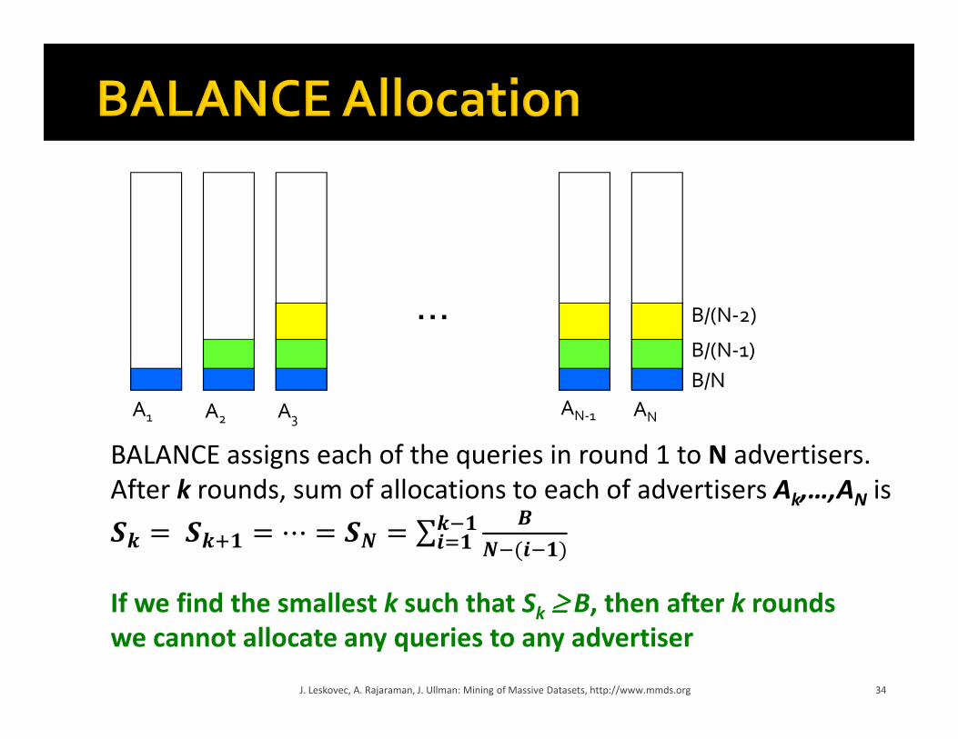
…
A1 A2 A3AN-1 AN
B/N
B/(N-1)
B/(N-2)
BALANCE assigns each of the queries in round 1 to N advertisers.
After k rounds, sum of allocations to each of advertisers Ak,…,AN is
� � �� ⋯ �� ∑�
�������
�����
If we find the smallest k such that Sk ≥≥≥≥ B, then after k rounds
we cannot allocate any queries to any advertiser
34J. Leskovec, A. Rajaraman, J. Ullman: Mining of Massive Datasets, http://www.mmds.org
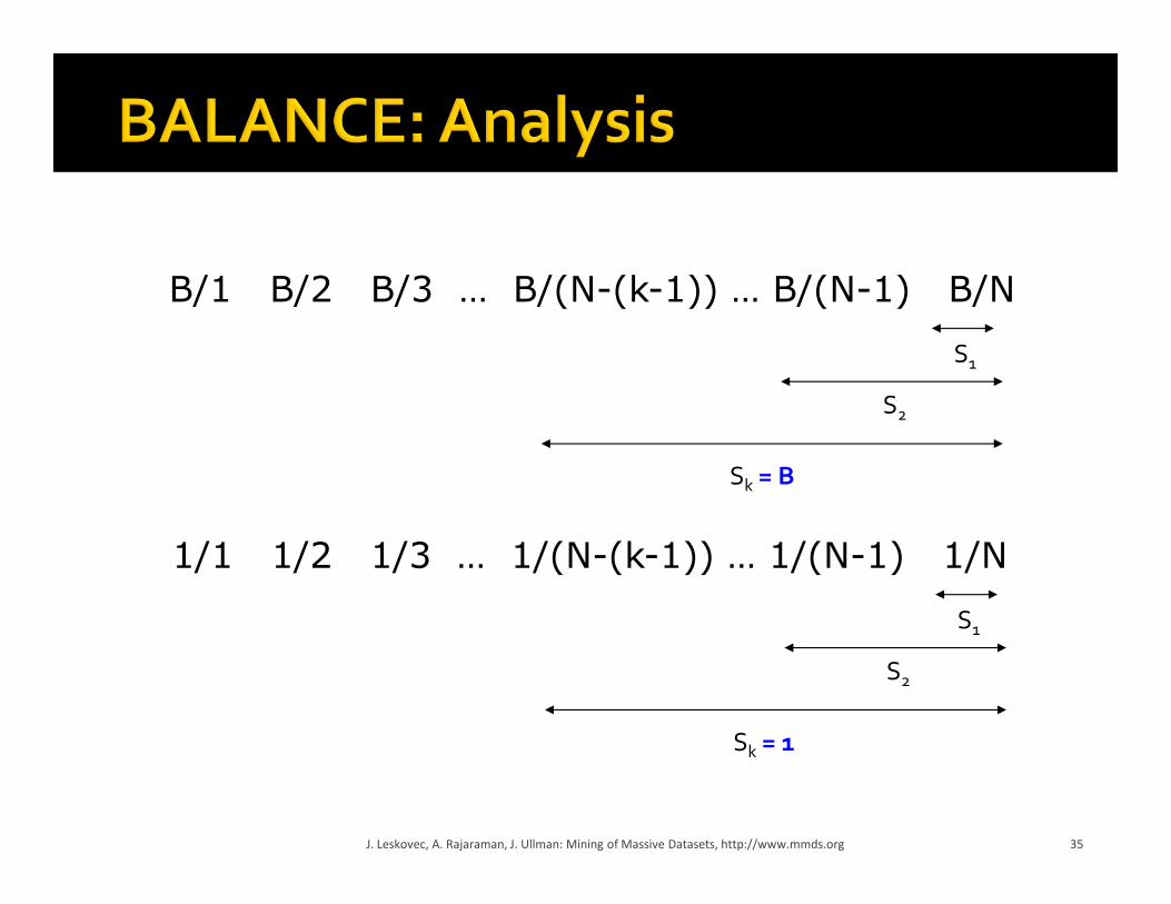
B/1 B/2 B/3 … B/(N-(k-1)) … B/(N-1) B/N
S1
S2
Sk = B
1/1 1/2 1/3 … 1/(N-(k-1)) … 1/(N-1) 1/N
S1
S2
Sk = 1
35J. Leskovec, A. Rajaraman, J. Ullman: Mining of Massive Datasets, http://www.mmds.org
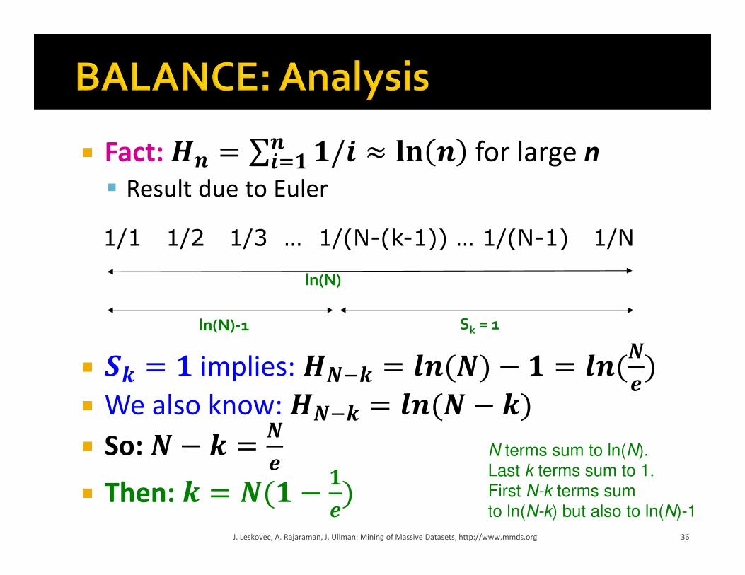
� Fact:�� ∑ �/����� � �� � for large n
� Result due to Euler
� � � implies: ��� ����� � � ����
��
� We also know: ��� ���� � �
� So: �� �
�
� Then: ��� ��
��
J. Leskovec, A. Rajaraman, J. Ullman: Mining of Massive Datasets, http://www.mmds.org 36
1/1 1/2 1/3 … 1/(N-(k-1)) … 1/(N-1) 1/N
Sk = 1
ln(N)
ln(N)-1
N terms sum to ln(N).
Last k terms sum to 1.
First N-k terms sum
to ln(N-k) but also to ln(N)-1
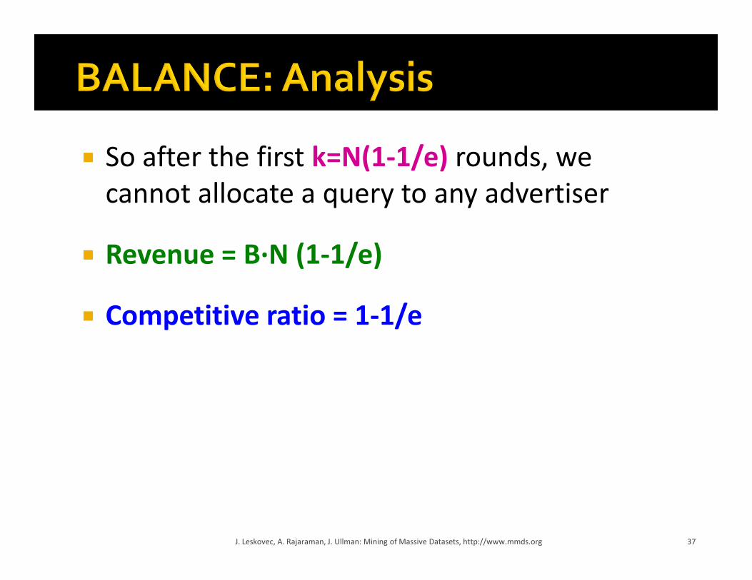
� So after the first k=N(1-1/e) rounds, we
cannot allocate a query to any advertiser
� Revenue = B∙N (1-1/e)
� Competitive ratio = 1-1/e
37J. Leskovec, A. Rajaraman, J. Ullman: Mining of Massive Datasets, http://www.mmds.org

� Arbitrary bids and arbitrary budgets!� Consider we have 1 query q, advertiser i
� Bid = xi
� Budget = bi
� In a general setting BALANCE can be terrible
� Consider two advertisers A1 and A2
� A1: x1 = 1, b1 = 110
� A2: x2 = 10, b2 = 100
� Consider we see 10 instances of q
� BALANCE always selects A1 and earns 10
� Optimal earns 100
38J. Leskovec, A. Rajaraman, J. Ullman: Mining of Massive Datasets, http://www.mmds.org
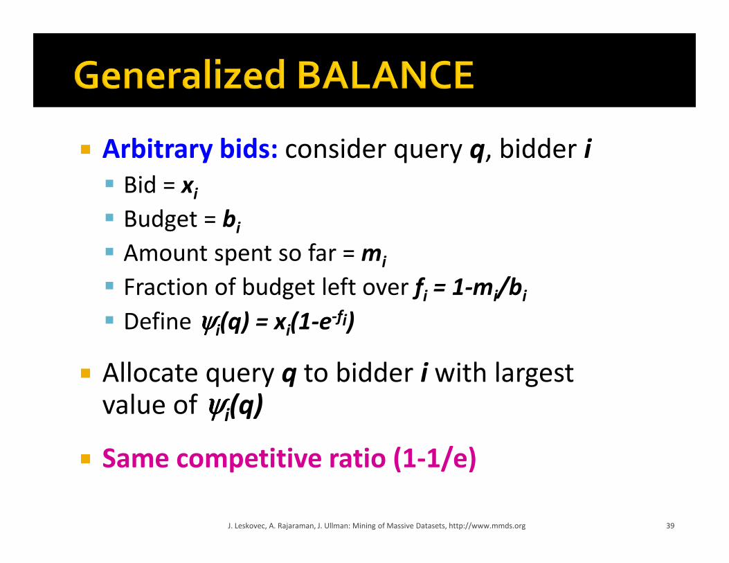
� Arbitrary bids: consider query q, bidder i
� Bid = xi
� Budget = bi
� Amount spent so far = mi
� Fraction of budget left over fi = 1-mi/bi
� Define ψψψψi(q) = xi(1-e-fi)
� Allocate query q to bidder i with largest value of ψψψψi(q)
� Same competitive ratio (1-1/e)
39J. Leskovec, A. Rajaraman, J. Ullman: Mining of Massive Datasets, http://www.mmds.org