cryptanalysis of rsa variants using small roots of polynomials
TRANSCRIPT

Cryptanalysis of RSA variants using small roots of polynomials
Citation for published version (APA):Jochemsz, E. (2007). Cryptanalysis of RSA variants using small roots of polynomials. Technische UniversiteitEindhoven. https://doi.org/10.6100/IR628814
DOI:10.6100/IR628814
Document status and date:Published: 01/01/2007
Document Version:Publisher’s PDF, also known as Version of Record (includes final page, issue and volume numbers)
Please check the document version of this publication:
• A submitted manuscript is the version of the article upon submission and before peer-review. There can beimportant differences between the submitted version and the official published version of record. Peopleinterested in the research are advised to contact the author for the final version of the publication, or visit theDOI to the publisher's website.• The final author version and the galley proof are versions of the publication after peer review.• The final published version features the final layout of the paper including the volume, issue and pagenumbers.Link to publication
General rightsCopyright and moral rights for the publications made accessible in the public portal are retained by the authors and/or other copyright ownersand it is a condition of accessing publications that users recognise and abide by the legal requirements associated with these rights.
• Users may download and print one copy of any publication from the public portal for the purpose of private study or research. • You may not further distribute the material or use it for any profit-making activity or commercial gain • You may freely distribute the URL identifying the publication in the public portal.
If the publication is distributed under the terms of Article 25fa of the Dutch Copyright Act, indicated by the “Taverne” license above, pleasefollow below link for the End User Agreement:www.tue.nl/taverne
Take down policyIf you believe that this document breaches copyright please contact us at:[email protected] details and we will investigate your claim.
Download date: 26. Feb. 2022

Dit proefschrift is goedgekeurd door de promotor:
prof.dr.ir. H.C.A. van Tilborg
Copromotor:dr. B.M.M. de Weger
CIP-DATA LIBRARY TECHNISCHE UNIVERSITEIT EINDHOVEN
Jochemsz, Ellen
Cryptanalysis of RSA variants using small roots of polynomials / door Ellen Jochemsz. –Eindhoven : Technische Universiteit Eindhoven, 2007.Proefschrift. – ISBN 978-90-386-1080-1NUR 919Subject headings : cryptology2000 Mathematics Subject Classification: 94A60, 12Y05, 11T71.
Printed by Printservice Technische Universiteit Eindhoven.Cover: Historical lattices. Design by Verspaget & Bruinink.

Cryptanalysis of RSA variants
using small roots of polynomials
proefschrift
ter verkrijging van de graad van doctor aan deTechnische Universiteit Eindhoven, op gezag van de
Rector Magnificus, prof.dr.ir. C.J. van Duijn, voor eencommissie aangewezen door het College voor
Promoties in het openbaar te verdedigenop donderdag 4 oktober 2007 om 16.00 uur
door
Ellen Jochemsz
geboren te Rijnsburg

Contents
1 Introduction 3
1.1 Cryptology, public key cryptography, and RSA . . . . . . . . . . . . . . . . 3
1.2 Overview of this work . . . . . . . . . . . . . . . . . . . . . . . . . . . . . 5
2 The RSA cryptosystem 9
2.1 Basics . . . . . . . . . . . . . . . . . . . . . . . . . . . . . . . . . . . . . . 9
2.2 RSA variants . . . . . . . . . . . . . . . . . . . . . . . . . . . . . . . . . . 10
2.3 Cryptanalysis . . . . . . . . . . . . . . . . . . . . . . . . . . . . . . . . . . 15
3 Small roots of polynomials 21
3.1 Preliminaries . . . . . . . . . . . . . . . . . . . . . . . . . . . . . . . . . . 21
3.2 Introduction to Coppersmith’s method . . . . . . . . . . . . . . . . . . . . 24
3.3 A general strategy for choosing the shifts . . . . . . . . . . . . . . . . . . . 30
3.3.1 Small modular roots . . . . . . . . . . . . . . . . . . . . . . . . . . 31
3.3.2 Small integer roots . . . . . . . . . . . . . . . . . . . . . . . . . . . 39
3.4 Tabular overview . . . . . . . . . . . . . . . . . . . . . . . . . . . . . . . . 44
3.5 Complexity of attacks using Coppersmith’s method . . . . . . . . . . . . . 46
4 Partial key exposure attacks on RSA 47
4.1 Introduction . . . . . . . . . . . . . . . . . . . . . . . . . . . . . . . . . . . 47
4.2 Known attacks . . . . . . . . . . . . . . . . . . . . . . . . . . . . . . . . . 48
4.3 A new “2-dimensional” attack . . . . . . . . . . . . . . . . . . . . . . . . . 53
4.3.1 Description of the new attack . . . . . . . . . . . . . . . . . . . . . 53
4.3.2 Special cases: Wiener and Verheul/van Tilborg . . . . . . . . . . . 57
4.3.3 Experiments for the new attack . . . . . . . . . . . . . . . . . . . . 59
4.4 New attacks up to full size exponents . . . . . . . . . . . . . . . . . . . . . 60
4.4.1 Polynomials derived from the RSA key equation . . . . . . . . . . . 62
4.4.2 Attacks for known MSBs and small d . . . . . . . . . . . . . . . . . 63
4.4.3 Attacks for known MSBs and small e . . . . . . . . . . . . . . . . . 67
4.4.4 Attack for known LSBs and small d . . . . . . . . . . . . . . . . . . 68
4.4.5 Experiments for the new attacks . . . . . . . . . . . . . . . . . . . . 68
4.5 Tabular overview . . . . . . . . . . . . . . . . . . . . . . . . . . . . . . . . 71
1

5 Attacks on RSA-CRT variants 73
5.1 Introduction . . . . . . . . . . . . . . . . . . . . . . . . . . . . . . . . . . . 73
5.2 Known attacks . . . . . . . . . . . . . . . . . . . . . . . . . . . . . . . . . 76
5.3 A new attack on CRT-Small-dp, dq . . . . . . . . . . . . . . . . . . . . . . . 82
5.3.1 A bound for a specific polynomial f with a small root . . . . . . . . 84
5.3.2 Description of the new attack . . . . . . . . . . . . . . . . . . . . . 85
5.3.3 Implementation of the new attack . . . . . . . . . . . . . . . . . . . 87
5.3.4 Experiments for the new attack . . . . . . . . . . . . . . . . . . . . 91
5.4 A new attack on CRT-Qiao&Lam . . . . . . . . . . . . . . . . . . . . . . . 95
5.4.1 A bound for a specific polynomial f with a small root . . . . . . . . 95
5.4.2 Description of the new attack . . . . . . . . . . . . . . . . . . . . . 96
5.4.3 Experiments for the new attack . . . . . . . . . . . . . . . . . . . . 97
5.5 Tabular overview . . . . . . . . . . . . . . . . . . . . . . . . . . . . . . . . 98
6 Attacks on Common Prime RSA 100
6.1 Introduction . . . . . . . . . . . . . . . . . . . . . . . . . . . . . . . . . . . 100
6.2 Known attacks . . . . . . . . . . . . . . . . . . . . . . . . . . . . . . . . . 100
6.3 A new attack on Common Prime RSA . . . . . . . . . . . . . . . . . . . . 104
6.3.1 Description of the new attack . . . . . . . . . . . . . . . . . . . . . 105
6.3.2 Experiments for the new attack . . . . . . . . . . . . . . . . . . . . 106
6.4 Tabular overview . . . . . . . . . . . . . . . . . . . . . . . . . . . . . . . . 107
7 Conclusion & open questions 108
7.1 The security of RSA: Advice for implementors . . . . . . . . . . . . . . . . 108
7.2 Open questions . . . . . . . . . . . . . . . . . . . . . . . . . . . . . . . . . 110
Bibliography 116
Index 123
Samenvatting 125
Summary 127
Acknowledgments 129
Curriculum Vitae 131
2

1Introduction
1.1 Cryptology, public key cryptography, and RSA
Cryptology , derived from the Greek word kryptos for “hidden” and logos for “word”, isoften defined as the study of secret writing. It is divided into two branches.
The first is cryptography which is mainly concerned with designing cryptosystems. Inhistory, cryptosystems were simply algorithms to encipher and decipher a message. In thecurrent days where computers are a major part of our industry, cryptography also providessolutions to many other security issues, such as authentication (for instance via digitalsignatures). A quote by the famous cryptographer Ron Rivest is that “cryptography isabout communication in the presence of adversaries”.
The second branch, cryptanalysis, deals with codebreaking, where an adversary triesto decrypt intercepted ciphertexts, or tries to find out who sent an anonymous message,or tries to pose as someone else, or tries to do any other thing that violates the goal of acryptosystem. Some might say that cryptanalysis is the “dark side” of cryptology, whileothers believe that researchers should try their best in breaking existing cryptosystems toprevent the real villains from finding the attacks first.
Methods to send messages in a secret way have been around since people started writing,and at the same time, people have been interested in deciphering secret messages. Thedevelopment of cryptography and cryptanalysis go hand in hand, and many times thecourse of history has been influenced by whether a cryptosystem used by a specific personor country was breakable or not [41, 67].
Up to 1976, almost all cryptosystems required that the sender and receiver shareda secret key. In these so-called symmetric cryptosystems, a message is encrypted by anencryption algorithm, which has both the message and the secret key as input. The outputis a ciphertext, that can be decrypted by a decryption algorithm, which has the ciphertextand the same secret key as input.
In 1976, Whitfield Diffie and Martin Hellman introduced1 the concept of asymmetriccryptography in their groundbreaking paper “New Directions in Cryptography” [23]. In
1In 1997 it became known that mathematicians of the British intelligence agency GCHQ had inventedasymmetric cryptography (James Ellis in 1970), a key exchange protocol analogous to Diffie and Hellman’s(Malcolm Williamson in 1974) and an asymmetric cryptosystem analogous to RSA (Clifford Cocks in 1973).
3

Introduction 1.1 Cryptology, public key cryptography, and RSA
this paper a key exchange protocol is introduced, which can be used by two people to agreeon a common secret key over an insecure channel. The paper also inspired the cryptocommunity to look for an asymmetric cryptosystem. That is, an encryption algorithmwhere the encryption key and the decryption key are not the same, and where the encryp-tion key can be published without giving away the information needed for decryption. In1978, Ron Rivest, Adi Shamir, and Len Adleman introduced the first asymmetric crypto-system, the RSA scheme [64]. Almost thirty years after its introduction, RSA is still themost used asymmetric cryptosystem in practice. The RSA scheme and its vulnerabilitiesare the main topic of this thesis.
In the setup phase of the RSA scheme in its simplest form, a person (whom we shall callAlice from here on) chooses two large prime numbers p and q and computes their productN = pq. Moreover, she selects a pair of integers (e, d) such that
ed ≡ 1 mod φ(N),
where φ(N) := (p− 1)(q − 1) is Euler’s totient function. Alice publishes (N, e) and keeps(p, q, d) private.
Another person (whom we shall call Bob) wishes to send a message m to Alice, wherem is represented as an element of Z∗N = (Z/NZ)∗. He knows e and N and can thereforeencrypt m by computing
c ≡ me mod N.
Bob sends the ciphertext c to Alice. Alice decrypts c by computing
cd ≡ med ≡ m1+kφ(N) ≡ m mod N.
The last equivalence, valid for all m that are coprime to N , is a result of Euler’s Theorem(which in turn is a generalization of Fermat’s Little Theorem). One can see that indeed,Alice recovers the message m using her secret decryption exponent d.
Since the introduction of RSA, it has become the most popular asymmetric crypto-system, and therefore much research has been done on its vulnerabilities (see for in-stance [8]). It is essential that the secret information (p, q, d) cannot be extracted efficientlyfrom the public information (N, e), since otherwise anyone could decrypt a message meantfor Alice. If the primes p and q are known, then φ(N) is known and it is easy to com-pute d using the Extended Euclidean Algorithm. Therefore, it is crucial that factoring themodulus N is hard, and many researchers are trying to factor large RSA moduli N . It isnot known if there exist integer factorization algorithms whose running time is polynomialin the bitsize of N . Currently, the best factoring algorithm, the Number Field Sieve, hasrunning time subexponential in the bitsize of N .
However, we may be able to factor an RSA modulus N if we can use additional in-formation. In this thesis, we focus on breaking RSA and RSA variants when an attackerhas some additional knowledge on the secret RSA parameters (p, q, d). For instance, anattacker could know that d is not chosen randomly, but selected in a special way. Or anattacker could know that there is a special relation between p and q. Such special designcriteria are not uncommon, since they can lead to a more efficient decryption or encryption.
4

Introduction 1.2 Overview of this work
Alternatively, an attacker could have obtained a part of the bits of the decryption exponentd by using a so-called side channel attack . A side channel attack is a physical attack onan RSA implementation, where an attacker tries to get information on d by connecting adevice to the computer or smartcard that is performing the RSA decryption (and measuringthe time it takes to run the decryption, or measuring the power consumption during thedecryption process).
The results in this thesis show that one must be very careful when using RSA or RSAvariants when the RSA parameters have special properties, or when part of the bits of dhave leaked. In essence, we show that in some of these variants, a multivariate polynomialappears which has a small root. Finding this small root means that secret RSA parametersof the system are fully exposed, and the factorization of N can be found.
This brings us to the theory (and practice) of finding small roots of polynomials. In1996, Don Coppersmith [14, 15, 16] introduced methods of finding small modular roots x0 ofunivariate polynomials fN(x) modulo some composite integer N , and finding small integerroots (x0, y0) of bivariate integer polynomials f(x, y). For the polynomials that appearin the cryptanalysis of RSA variants, we sometimes need extensions of Coppersmith’smethods to more variables. These extensions are heuristic, in the sense that they relyon an assumption, which turns out to work well in practice, but which must always betested for specific attack scenarios. The methods enable us to analyze for each polynomialthat occurs in an RSA variant, how small the root should be such that it can be found intime polynomial in the bitsize of N . In this way, we can see in which cases the additionalinformation that the attacker has is enough to obtain the factorization of N in polynomialtime.
1.2 Overview of this work
Now that we have introduced the topic of the thesis, we are ready to state our main goal,and give an overview of the thesis and our contributions.
Research goal:
We aim to design new attacks on RSA and RSA variants, which allow us tofactor the RSA modulus N in time polynomial in the bitsize of N .
In the design of these new attacks, the assumption is made that an attackerhas some information on the secret RSA parameters of the system, eitherobtained from e.g. a side channel attack, or by knowing special design criteriaof the RSA variant.
5

Introduction 1.2 Overview of this work
Motivation of the research:
Let us briefly discuss the motivation for exploring attacks on RSA in which an attackerhas some extra information on the RSA parameters.
As we shall see later, side channel attacks are a serious threat to RSA implementa-tions. These attacks exploit physical characteristics such as the running time or the powerconsumption of a decryption procedure, to draw conclusions about the bits of the secretkey d. This may lead to partial leakage of the bits of d, and raises the question whetheror not this information is enough for an attacker to recover the rest of d.
The other attacks that we deal with, namely attacks on RSA variants that have specialdesign criteria, are motivated by the various proposals to speed up RSA. Since RSA is apopular system, researchers are always interested in achieving a more efficient encryptionor decryption procedure by choosing the RSA parameters in a special way.
Organization of this thesis and our main contributions:
Chapter 2: The RSA cryptosystem
In Chapter 2, we outline the RSA scheme and variants on RSA, and introduce differentways to mount attacks. Moreover, we show that in some of the cryptanalytic results onRSA, polynomials with small roots are used. We end this chapter by introducing twoimportant attacks on RSA with small decryption exponent d, by Wiener [75] and Bonehand Durfee [10].
Chapter 3: Small roots of polynomials
Since polynomials with small roots play an important role in the cryptanalysis of RSA,we deal with this topic in a separate chapter (Chapter 3). We introduce Coppersmith’smethods of finding small modular roots of univariate polynomials, and of finding smallinteger roots of bivariate polynomials [14, 15, 16]. We explain how the methods can beextended to more variables, although the techniques will become heuristic in these cases.We will also use the works of Howgrave-Graham [35] and Coron [18], who revisited Copper-smith’s methods for small modular roots and small integer roots respectively.
One difficulty in applying a Coppersmith method to a new multivariate polynomial fthat appears in cryptanalysis, is the choice of the so-called shift polynomials. This choicedepends on the monomials that appear in f . We present a general strategy that can befollowed, which prescribes which shift polynomials can be used. The general strategy canalso be used to give an easy answer to the question: How small should the root be suchthat it can be found in polynomial time? For small integer roots, this strategy is a gene-ralization of a strategy by Blomer and May for bivariate polynomials [7].
Parts of this chapter are based on [37], presented at Asiacrypt 2006, which is joint workwith Alexander May.
6

Introduction 1.2 Overview of this work
Chapter 4: Partial key exposure attacks on RSA
In Chapter 4, we introduce the concept of partial key exposure, which is the situation thatan attacker has obtained a part of the bits of the secret exponent d. We describe the knownpartial key exposure attacks on RSA by Boneh, Durfee, and Frankel [12] and by Blomerand May [6], and present new ones.
The first new attack deals with the case that d is chosen to be small. In the nineties,it was shown by Wiener [75] that a private exponent d can be found if d < N
14 . Verheul
and van Tilborg [72] show that Wiener’s attack can be extended slightly to d < N14+ε for
a small ε, but at the cost of a workload of O(N2ε). Our new partial key exposure attackuses a 2-dimensional lattice and is an extension of the attacks by Wiener and Verheul/vanTilborg to the case of partial key exposure.
The attacks that we describe next show that partial key exposure attacks on RSA existwhenever either d or e is chosen to be significantly smaller than φ(N).
Parts of this chapter are based on [36], presented at ISC 2006, which is joint work withBenne de Weger. Other parts of the chapter are based on [25], presented at Eurocrypt 2005,a joint paper with Matthias Ernst, Alexander May, and Benne de Weger.
Chapter 5: Attacks on RSA-CRT variants
The most popular variant of RSA is called RSA-CRT, which only involves a small changein the decryption process. Instead of computing cd mod N directly, one could use so-calledCRT-exponents dp ≡ d mod (p− 1) and dq ≡ d mod (q − 1). Then by combining
mp ≡ cdp mod p and mq ≡ cdq mod q
using the Chinese Remainder Theorem (CRT), one can also find the original message m.A gain in efficiency is caused by the fact that the private CRT-exponents dp and dq (andall the other numbers that occur in the process of the modular exponentiation) are the sizeof p and q instead of the size of N .
Moreover, it may be tempting to choose dp and dq significantly smaller than p and qto obtain an even faster decryption phase. Wiener suggested to use these small privateCRT-exponents instead of small private exponents in the paper where he attacked d < N
14 .
It has been an open question since whether or not there exist polynomial time attacks onRSA-CRT with small CRT-exponents. In Chapter 5, we answer this question and showthat there is an attack on RSA-CRT if dp and dq are smaller than N0.073.
In a variant on RSA-CRT it is proposed to choose dq = dp − 2, such that a user onlyhas to store one of the private CRT-exponents. We show that this is unsafe if dp < N0.099.
These new attacks are an addition to the known attacks on RSA-CRT variants byMay [52], Bleichenbacher and May [4], Galbraith, Heneghan, and McKee [27] and Sun,Hinek, and Wu [69].
Parts of this chapter are based on [38], presented at Crypto 2007, others are based on [37],presented at Asiacrypt 2006. Both papers are joint work with Alexander May.
7

Introduction 1.2 Overview of this work
Chapter 6: Attacks on Common Prime RSA
Another variant on RSA, called Common Prime RSA, is the topic of Chapter 6. In thisvariant, the primes p and q satisfy a special relation, which causes Wiener’s attack to workless well. Therefore, by choosing the primes in this special way, one is able to use a de-cryption exponent d smaller than N
14 . We discuss the known attacks collected in a paper
by Hinek [32]. We show a new attack on Common Prime RSA which significantly restrictsthe number of safe choices for d.
Parts of this chapter are based on [37], presented at Asiacrypt 2006, which is joint workwith Alexander May.
Chapter 7: Conclusions & open questions
Finally, we conclude with an overview of the security of RSA and its variants, and provideguidelines for designers and implementors of new RSA variants. Moreover, we address anumber of open questions, either related to finding small roots of polynomials, or to RSAcryptanalysis.
8

2The RSA cryptosystem
In this chapter, we introduce the RSA cryptosystem and some variants on it. Most ofthese variants were proposed in attempts to speed up either the encryption phase or thedecryption phase of RSA. We describe the various ways to attack RSA schemes in thesection on cryptanalysis of RSA.
2.1 Basics
The standard RSA scheme [64] is built up as follows.Let n be a security parameter, usually called the modulus length. Let p and q be two
randomly generated primes of about 12n bits. Take N := pq to be the n-bit RSA modulus.
Typically, n = 1024, although n = 2048 is used in practice by more conservative users.Next, one generates two integers e and d which are each other’s inverse modulo φ(N) =
(p − 1)(q − 1). This can be done by choosing either e or d at random, coprime to φ(N),and computing the other integer using the Extended Euclidean Algorithm. This algorithm,when performed on an integer pair (a1, a2), finds integers b1 and b2 such that
a1b1 + a2b2 = gcd(a1, a2).
So, when for instance (e, φ(N)) is taken as an input, one finds b1 and b2 such that
eb1 + φ(N)b2 = 1.
Take b1 = d and b2 = −k. Then an integer pair (e, d) can be found such that
ed = 1 + kφ(N).
When Alice has generated the parameters of her RSA system, then the public key crypto-system works as follows. Alice publishes (e,N) and keeps (p, q, d) secret. If Bob wants tosend a message to Alice, he represents it as an integer m ∈ (1, N) that is coprime to N .He then encrypts m by computing
c ≡ me mod N,
which is possible since he knows both e and N .
9
The RSA cryptosystem 2.2 RSA variants
Alice can decrypt the message by computing
cd ≡ med ≡ m1+kφ(N) ≡ m mod N.
Aside from being an encryption scheme, RSA can also be used as a digital signaturescheme. This is important when authentication of the sender of a message is requested.Suppose Alice wants to prove that a certain message is written by her. She can thencompute
s ≡ md mod N
using her private exponent d, and send the signature s, together with the message m.Then, anyone can compute
se ≡ med ≡ m1+kφ(N) ≡ m mod N,
and check if the output of this computation corresponds to the message m accompanyingthe signature. This is called the verification of the signature s.
In practice, it is often not the message itself that gets signed, but a condensed versionof m, the outcome of a hash function H when performed on m. Naturally, anyone can verifythat H(m) = se mod N is the hash value of the corresponding m if the hash function ispublicly known.
2.2 RSA variants
Since its introduction in 1978, RSA has become a widely used cryptosystem. There-fore, many people have tried to speed up the process of encrypting/verifying or decrypt-ing/signing a message.
Let us first examine the efficiency of these processes in the case of standard RSA.A standard way to perform this modular exponentiation is by the ‘Square-and-MultiplyMethod ’, also known as the ‘Repeated Squaring Method’. In order to compute me mod N ,one first looks at the bit representation of e, that is (en−1, . . . , e0), for e =
∑n−1i=0 ei2
i. So,
me = me0+2(e1+2(e2+2(e3+...))).
One can compute me mod N in an iterative way by setting initial values x = 1, y = m,and for i = 0, 1, . . . , n− 1:
• if ei = 1 then put x = x · y mod N ,
• if i < n− 1, then put y = y2 mod N .
After these iterations, output x = me mod N . In total, this so-called ‘right-to-left’ methodinvolves as many squarings as the bitsize of e and as many multiplications as there areones in the bit representation of e.
10

The RSA cryptosystem 2.2 RSA variants
Each multiplication or squaring can be performed in time c ·n2, where c is a constant. Weconclude that the total method takes at most time 2 · bitsize(e) · cn2 ≤ 2cn3. Equivalently,the time for the decryption process is at most 2 · bitsize(d) · cn2 ≤ 2cn3.
Next, we will describe a number of proposed variants on RSA. Most of them focus onspeeding up either the encryption (or signature verification) phase or the decryption (orsigning) phase of the cryptosystem.
RSA with small public exponent e (“Small-e”):
RSA with a small encryption exponent e occurs often in practice. Since the encryptionexponent is public, one can choose it to be for instance e = 3 or e = 216 + 1, which are themost common choices. For e = 3, only two multiplications and one squaring are requiredfor the exponentiation in the encryption phase. For e = 216 + 1, the number of multiplica-tions and squarings are 2 and 16 respectively. In the case of RSA-Small-e, a small e is firstfixed in the key generation (after the random choices of p and q have been made). Then,the Extended Euclidean Algorithm computes the corresponding d, which will be ‘full size’(that is, about the same bitsize as φ(N)) in general.
RSA with small private exponent d (“Small-d”):
If a fast decryption/signing phase is needed, for instance on constrained devices like smart-cards, one could use RSA with a small private exponent d. In that case, first d can bechosen to be of a certain size, after which the corresponding e is determined by the Ex-tended Euclidean Algorithm. In general, e will be ‘full size’ in this case. As we shall see inthe next section on cryptanalysis of RSA, Wiener [75] showed in 1990 that there are poly-nomial time attacks on RSA with small d. Namely, he showed that d can be found in timepolynomial in n = bitsize(N) if d < N
14 . Boneh and Durfee extended this attack bound to
d < N0.292 in 2000 [10]. With n = 1024, this is already a much stronger attack than thebrute force attack and meet-in-the-middle attack that will be described in Section 2.3.
Standard RSA-CRT (“CRT-Standard”) :
A standard way to speed up RSA decryption, as proposed by Quisquater and Couvreur [61],is by splitting up the exponentiation in the decryption phase and using the Chinese Re-mainder Theorem. That theorem says that if two integers r and s are coprime, and weknow integers a1, a2 such that
x ≡ a1 mod r, x ≡ a2 mod s,
then the unique x < rs that satisfies both equations can be constructed efficiently.Instead of computing cd mod N directly, one could use so-called private CRT-exponents
dp ≡ d mod (p− 1) and dq ≡ d mod (q − 1). Then by combining
mp ≡ cdp mod p and mq ≡ cdq mod q
using the Chinese Remainder Theorem, one can also find the original message m.
11

The RSA cryptosystem 2.2 RSA variants
Since bitsize(dp) = bitsize(dq) = 12n, each of these exponentiations will involve 1
2n squarings
and at most 12n exponentiations, so the total number of squarings and multiplications stays
the same as in the standard case (but the operands are shorter). A squaring or multiplica-tion modulo p takes time at most c ·(bitsize(p))2 = 1
4cn2. Therefore, if one neglects the time
used for the Chinese Remainder Theorem, then it can be concluded that decryption withthe Quisquater/Couvreur method is four times faster than the decryption in standard RSA.
RSA-CRT with small public exponent e (“CRT-Small-e”) :
As in standard RSA, it is possible to choose a small e, after which the Extended EuclideanAlgorithm finds the corresponding d, which in turn is split up in dp and dq. This is pro-bably the most popular variant of RSA in practice. If one chooses p and q at random, andthen a small e, then the private CRT-exponents dp and dq will be about as long as p andq in general.
RSA-CRT with small private CRT-exponents dp, dq (“CRT-Small-dp, dq”) :
Similarly, it is also possible to choose small private CRT-exponents dp and dq. After fixingdp and dq, one needs to compute d smaller than φ(N) = (p− 1)(q − 1) such that
d ≡ dp mod (p− 1) and d ≡ dq mod (q − 1).
Since p − 1 and q − 1 are not coprime, one cannot use the Chinese Remainder Theoremdirectly. However, one could do the following.
Pick random primes p, q of the same bitlength such that gcd(p− 1, q− 1) = 2. Chooserandom odd integers dp, dq of the same small size, that is dp, dq < Nβ for some β ∈ (0, 1
2).
Use the Chinese Remainder Theorem to compute the unique x < (p−1)(q−1)4
that satisfies
x ≡ dp − 1
2mod
p− 1
2and x ≡ dq − 1
2mod
q − 1
2.
Then for d = 2x + 1, it holds that d ≡ dp mod (p − 1) and d ≡ dq mod (q − 1). Fromthis d, one can compute the corresponding e as usual.
Wiener suggested to use these small private CRT-exponents instead of small private ex-ponents in the paper where he attacked d < N
14 . It has been an open question since whether
or not there exist polynomial time attacks on RSA-CRT with small CRT-exponents.
RSA-CRT with unbalanced primes (“CRT-UnbalancedPrimes”) :
In a study of RSA-CRT cases that can be broken, May designed the concept of RSA-CRTwith unbalanced primes [52]. We know that in RSA-CRT, the equations
edp ≡ 1 mod (p− 1), edq ≡ 1 mod (q − 1)
hold. Suppose that q = Nβ for some β ∈ (0, 12) is the smaller of the two prime factors
of N . This implies that the exponentiation modulo q is relatively fast. Now one could alsomake the exponentiation modulo p fast by choosing dp to be small. This is basically thevariant that May proposes:
12

The RSA cryptosystem 2.2 RSA variants
• have a modulus that is the product of unbalanced primes p, q with p > q,
• choose dq randomly (so dq will be about as large as the ‘small’ prime q), and
• choose a small dp to speed up the exponentiation modulo the ‘large’ prime p.
RSA-CRT with small e and small dp and dq (“CRT-BalancedExponents”) :
In 2005, two independent papers [28, 70] proposed the same RSA variant, namely one thatuses RSA-CRT in which both e and dp and dq are smaller than standard. Let us show howthis can be achieved in the key generation phase. We want e, dp, dq, p, q, kp, kq such that
edp = 1 + kp(p− 1), edq = 1 + kq(q − 1),
with e of bitsize αn, dp and dq of bitsize βn, and p and q of bitsize 12n. Here, α ∈ (0, 1)
and β ∈ (0, 12). By this construction, kp and kq are of bitsize (α + β − 1
2)n.
First, one chooses random dp, dq of the right bitsize, and kp, kq of the right bitsizesatisfying gcd(dp, kp) = gcd(dq, kq) = gcd(kp, kq) = 1. Next, one computes e′ using CRTsuch that
e′ ≡ d−1p mod kp and e′ ≡ d−1
q mod kq.
Since e′ is now smaller than kpkq which is (2α+2β−1)n bits, compute e := e′+ c ·kpkq for
some c of bitsize (1−α−2β)n. Finally, put p := edp−1
kpand q := edq−1
kq, and check if p and q
are both prime. If not, repeat the whole procedure until the p and q that are obtained areboth prime.
Note that c must be positive, so it is needed that α < 1 − 2β. This key generationalgorithm is a slight variation to the one proposed by Galbraith/Heneghan/McKee [28]. Intheir algorithm, they first choose e, kp, and kq, and then compute dp and dq as the inversesof e mod kp and mod kq. This requires dp > kp and dq > kq, and thus α < 1
2, which is
quite restrictive. However, if α < 12, then the method of [28] should be preferred, since one
can generate p and q separately, and the method does not rely on two integers that haveto be prime at the same time.
The key thing to note in the generation of these balanced exponents is the fact that pand q are generated last (and then tested for primality). Hence, the modulus N is a productof two special primes instead of two randomly chosen ones, and therefore the number ofpossible N is less than usual, but it is unknown whether this can be exploited.
RSA-CRT with small difference dp − dq (“CRT-Qiao&Lam”) :
In a proposal to save on both memory and decryption time on constrained devices likesmartcards, Qiao and Lam [60] proposed to use RSA-CRT with small dp, and to usedq = dp− 2. In this way, one profits from the fast decryption method of CRT-Small-dp, dq,while one has to store only one of the two private CRT-exponents.
13

The RSA cryptosystem 2.2 RSA variants
RSA with special p, q (“Small Prime Difference”, “Common Prime”, etc.):
Some settings of RSA have primes p and q that are generated in a special (non-random)way, either because of a faulty implementation, or on purpose. Examples include:
• A small prime difference p− q:It is known that it is unsafe to use primes with a small prime difference. BesidesFermat’s factoring attack (see for instance [74]), there are attacks on the RSA settingwith small d and a small prime difference by de Weger [74].
• Primes p, q such that gcd(p− 1, q − 1) = 2g, for g a large prime:As we shall see in Chapter 6, the attacks by Wiener and Boneh/Durfee on small dwork less well for this variant called Common Prime RSA. Therefore, it might bepossible to use a d < N
14 if g, the prime factor that p − 1 and q − 1 are sharing, is
large enough (though not too large, to avoid other attacks).
• Primes p and q that share a block of least significant bits:As we shall see in Chapter 4, this variant makes a partial key exposure attack byBoneh, Durfee, and Frankel harder to perform, and was therefore proposed as aninteresting RSA variant by Steinfeld and Zheng [68].
• Partial knowledge of the primes p and q:A consequence of the variant by Steinfeld and Zheng that we have just sketchedis that an attacker can find the least significant bits that p and q share. In anyvariant where an attacker knows a set of either most significant bits (MSBs) or leastsignificant bits (LSBs) of one of the secret primes p and q, one must beware of animportant result by Coppersmith [16]. This result states that N can be factored
efficiently if the known MSB or LSB part of p is at least as big as N14 . This result
will be discussed in Section 4 (in Theorem 4.1), since it is also the basis of the firstpartial key exposure attacks on RSA by Boneh, Durfee, and Frankel [12].
RSA with moduli N = p1 · . . . · pr or N = prq (“Multi-prime”/“Takagi”):
We have already mentioned that the decryption/signing process in RSA can be made moreefficient by performing exponentiations modulo the prime factors of N , and then combiningthese with the Chinese Remainder Theorem. It follows easily that using RSA with more,and smaller prime factors should improve the efficiency of this decryption phase even more.
Therefore, RSA variants have been proposed that use N = p1 · . . . · pr, where the pi aredistinct primes of equal bitsize, or N = prq, for primes p and q of equal bitsize and r asmall integer. The first variant is called “Multi-prime RSA”, the second “Takagi’s RSA”(also known as “Multi-power RSA”) since it was proposed by Takagi [71]. Obviously, onenecessary (though not sufficient) condition is that the prime factors are large enough toavoid attacks using the factorization methods.
14

The RSA cryptosystem 2.3 Cryptanalysis
2.3 Cryptanalysis
As there are many different ways to attack RSA, we divide the attacks into the followingcategories:
1. Factoring N :Given an RSA modulus N of bitsize n, the goal is to find its prime factorization.In these attacks, an adversary gets no public exponent e, no ciphertext c, only thecomposite integer N . Currently, the best (general) factorization method, the NumberField Sieve [47], has a number of bit operations that is bounded by
exp((1.902 + o(1)) ln(N)
13 (ln(ln(N)))
23
)
for N →∞. In special cases, namely when one is looking for a small prime factor ofa number N , the Elliptic Curve Method (ECM) [49] could be used. Currently, thelargest factor found by the ECM has 222 bits. We refer to [46] for more details oninteger factorization.
2. Brute force and meet-in-the-middle attacks on d or dp, dq:The brute force and meet-in-the-middle attacks on d (or, in the RSA-CRT case, dp
and dq) show that one should choose these secret values large enough such that anattacker is not able to find them by simply trying all possibilities. If a message m isvery small, then one might try to encrypt all possible plaintexts m with the publicexponent e, and check if the result is an intercepted ciphertext. Similarly, if one knowsthat d is chosen small, one might try all possibilities for d to decrypt the ciphertext.All of these attacks are so-called brute force attacks, and are simply attacks usingexhaustive search. To say that a certain parameter choice is safe against brute forceattacks, we need to quantify the maximal amount of operations that an attacker isable to perform. A usual choice for this is 280 (see for instance report on the hardnessof computational problems in cryptography [24], where it is said that an exhaustivesearch of 80 bits is on the edge of what is not doable today). Hence, all secret RSAparameters should be at least 80 bits long to avoid brute force attacks.
A more advanced category of attacks is called meet-in-the-middle attacks. In theseattacks, there is a trade-off between storage and running time. For a detailed descrip-tion of meet-in-the middle attacks on RSA and RSA-CRT, we refer to [51]. Here, weshow how it works on a small d. Given a message-ciphertext pair (m, c), such thatc ≡ me mod N , assume that e’s inverse d has an upper bound D. Then, d is builtup as
d = d√
De · d0 + d1.
Make a sorted list of all couples (d0, cd√De·d0) for d0 <
√D. For d1 running from 0 to√
D, compute m · (c−1)d1 , and check if (d0,m · (c−1)d1) in the list. If so, then outputd = d√De · d0 + d1. Hence, at the cost of a list with about
√d entries, the number
of tries to find d can be reduced to about√
d.
15

The RSA cryptosystem 2.3 Cryptanalysis
3. Attacks that involve plaintext-ciphertext pairs (m, c):These attacks use the knowledge that ciphertexts c are computed as the e-th power ofan unknown message m modulo N . Therefore, they fall into the category of so-called“message recovery attacks”, instead of the “key-recovery attacks” that are the maintopic of this thesis. Examples include
• Hastad attack [31]: It is unsafe to send the same message m to more recipientsthat all use RSA with e = 3 (although they have different moduli).
• Franklin-Reiter attack [17]: With e = 3, it is unsafe to send related messagesm1, m2, with m1 ≡ f(m2) mod N for some linear polynomial f .
• Coppersmith short pad attack [16]: Suppose two messages m1 and m2 areessentially the same message m, but concatenated with different (unknown)paddings r1 and r2. If the paddings are at most b = bn/e2c bits long, and theoriginal message m is at most n− b bits, then an attacker can find m from theciphertexts, e and N .
All of the above attacks are described in Boneh’s survey paper [8].
4. Implementation attacks :Even if a cryptosystem is flawless in theory, vulnerabilities can arise when it is im-plemented.
• Side channel attacks: Side channel attacks take advantage of implementation-specific characteristics to recover the secret exponent d that is involved in thecomputation of a decryption or signature. This characteristic information canbe extracted by timing the decryption/signing process, by examining the powerconsumption of the process, etc. In the case of RSA, this could mean thatan attacker examines the power consumption of a device that is applying theSquare-and-Multiply Method for the decryption, and tries to distinguish periteration if a squaring and a multiplication occur (di = 1) or if only a squaringoccurs (di = 0).
These types of attacks have become an important part of the research on RSAsecurity in practice, since Kocher introduced his timing attacks [42] in 1996.Other main results in the area include the introduction of simple and differentialpower analysis [43] by Kocher, Jaffe, and Jun, and the introduction of attackingimplementations by inducing faults in specific iterations by Boneh, DeMillo, andLipton [9]. For an overview on side channel attacks, we refer to [62, 39]. Forthe motivation of the research in Chapter 4, on partial key exposure attacks, itis important to remark that some side channel attacks are able to reveal only apart of the secret exponent d [22].
16

The RSA cryptosystem 2.3 Cryptanalysis
• Bleichenbacher’s first attack on PKCS-1: In an old version of PKCS-1 (PublicKey Cryptography Standard 1), an encryption of a message m was in fact anencryption of the following data string:
02 random padding 00 m
In [3], Bleichenbacher shows that this causes problems when a protocol de-crypting a ciphertext c outputs an error message when the initial block does notconsist of the bytes 0 and 2. Basically, an attacker can intercept a ciphertext c,and send c′ ≡ rc mod N to be decrypted, for some random r.
Now the attacker will learn whether or not the 16 most significant bits are equalto 02. Hence, the attacker has a method that tells him if the decryption of achosen ciphertext has the correct initial block. Bleichenbacher shows that thisis enough to decrypt c.
• Bleichenbacher’s second attack on PKCS-1: At the rump session of Crypto’06,Bleichenbacher showed another attack on an implementation of PKCS-1, whichshows that in some cases, an RSA signature can be forged if a public exponente = 3 is used. In order for an RSA signature to be accepted, it must look like
standard PKCS-1 padding bytes in ASN.1 format hash of the signed data
after the cube root of the signature is taken. The second block indicates whichhash algorithm is used, and how long the hash value is. Now the attack appliesto implementations of this signature verification that fail to check if there arebits in the data string after the hash. If one can submit a signature of whichthe cube root is
standard PKCS-1 padding bytes in ASN.1 format hash extra bits
then the signature is accepted as valid. An attacker can choose the extra bitsfreely in order to create a perfect cube.
5. Factoring N with extra information on the RSA parameters :These attacks are the main topic of this thesis. We have seen in the previous sectionthat many RSA variants have special design criteria, that can help an adversaryperform an attack. Also, as a result of the side channel attacks mentioned above, itis possible that an adversary has learned a part of the bits of d. Then, we could askin which cases this so-called partial key exposure is enough to retrieve the rest of d.As opposed to the attacks in category 2 of this list, we do not use encryptions c ofmessages m. Instead, we focus on the known relations between the RSA parameters,such as the so-called RSA key equation
ed = 1 + kφ(N), or equivalently: ed = 1 + k(N + 1− (p + q)).
17
The RSA cryptosystem 2.3 Cryptanalysis
In the chapters that follow, many known attacks will be described on the RSA variants,preceding the description of the new attacks that we have found on these variants. Thenew attacks include partial key exposure attacks on RSA-Small-e and RSA-Small-d, thefirst polynomial time attack on RSA-CRT-Small-dp, dq, and new attacks on RSA-CRT-Qiao&Lam and Common Prime RSA.
Since this work does not contain new attacks on RSA with small prime difference,Multi-prime RSA or Takagi’s RSA, we refer to [74], [33], and [13, 55] respectively forrecent attacks on these variants.
We now proceed by introducing the two most important known attacks in this area,namely the attacks by Wiener [75] and Boneh and Durfee [10] on RSA-Small-d.
Wiener’s Attack:
In 1990, Wiener showed the following result.
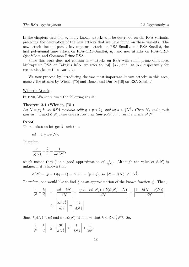
Theorem 2.1 (Wiener, [75])
Let N = pq be an RSA modulus, with q < p < 2q, and let d < 13N
14 . Given N , and e such
that ed = 1 mod φ(N), one can recover d in time polynomial in the bitsize of N .
Proof.There exists an integer k such that
ed = 1 + kφ(N).
Therefore,
e
φ(N)− k
d=
1
dφ(N),
which means that kd
is a good approximation of eφ(N)
. Although the value of φ(N) isunknown, it is known that
φ(N) = (p− 1)(q − 1) = N + 1− (p + q), so |N − φ(N)| < 3N12 .
Therefore, one would like to find kd
as an approximation of the known fraction eN
. Then,
∣∣∣∣e
N− k
d
∣∣∣∣ =
∣∣∣∣ed− kN
dN
∣∣∣∣ =
∣∣∣∣(ed− kφ(N)) + k(φ(N)−N)
dN
∣∣∣∣ =
∣∣∣∣1− k(N − φ(N))
dN
∣∣∣∣
≤∣∣∣∣∣3kN
12
dN
∣∣∣∣∣ =
∣∣∣∣3k
dN12
∣∣∣∣ .
Since kφ(N) < ed and e < φ(N), it follows that k < d < 13N
14 . So,
∣∣∣∣e
N− k
d
∣∣∣∣ ≤∣∣∣∣
3k
dN12
∣∣∣∣ <
∣∣∣∣1
dN14
∣∣∣∣ <1
3d2.
18

The RSA cryptosystem 2.3 Cryptanalysis
At this point, we need to recall some facts from the theory of continued fractions. Thecontinued fraction representation of a real number x is [a0, a1, . . .] for
x = a0 +1
a1 + 1a2+...
.
The fraction
pi
qi
= [a0, . . . , ai] = a0 +1
a1 + 1a2+ 1
...+ai
is called the ith convergent of x.A classical theorem by Legendre [45] (for a recent reference, see [30, Theorem 184])
states that all fractions ab
such that
∣∣∣x− a
b
∣∣∣ <1
2b2
are obtained as convergents of x. Since k and d are coprime, kd
can be found as one of theat most n = bitsize(N) convergents of e
N.
2
In Section 1.1, we have mentioned that we focus on attacks on RSA which factor N inpolynomial time when we are given extra information on the secret parameters. However,we have only shown so far that one can recover d in polynomial time. After applyingWiener’s attack, finding the factorization of N is easy, since we know both d and k, so wecan find the correct value of φ(N) = N + 1− (p + q) after which we can solve p, q from
{φ = N + 1− (p + q),N = pq.
Suppose we could only retrieve d and not k in polynomial time. A proof of the followingtheorem, stating that knowledge of d also allows one to factor N in polynomial time, canbe found in [8].
Theorem 2.2Let N = pq be an RSA modulus. Suppose integers e, d > 1 are known such that ed ≡ 1mod φ(N). Then N can be factored in probabilistic polynomial time.
Here, probabilistic polynomial time means that the method involves a random g ∈ Z∗N ,and succeeds in finding the factorization of N (in polynomial time) with probability atleast 1
2. If the factorization fails, one simply has to try other choices for g.
Recently, May showed that this equivalence of finding d and factoring N is deterministicpolynomial time for balanced primes [54], which was extended to the case of unbalancedprimes by Coron and May in [20].
19

The RSA cryptosystem 2.3 Cryptanalysis
Boneh/Durfee’s Attack:
Ten years after the publication of Wiener’s attack, Boneh and Durfee showed an improve-ment on the attack bound to d < N0.292 [10].
Their method is not based on continued fractions, but is one of the first that is basedon the theory of finding small roots of polynomials by Coppersmith. This method involveslattices and lattice basis reduction, and resultants or Grobner bases. Often, the attacksthat use the method are not provable but heuristic, although the heuristic seems to performwell in practice. Since Coppersmith’s work on finding small roots of polynomials is thetopic of the next chapter, we will treat Boneh and Durfee’s attack in detail later.
For now, we shall only show which polynomial with a small root appears in the attackof Boneh and Durfee. It is derived directly from the RSA key equation, namely
ed = 1 + k(N − (p + q − 1)).
Suppose one looks at this equation modulo e, and replaces k and p+q−1 by the unknownsx and y. Then, one would like to find the root (x0, y0) = (k, p + q − 1) of the polynomialfe(x, y) = 1 + x(N − y) modulo e. The root can be considered ‘small’ since
|x0| = |k| < d = Nβ and |y0| = |p + q − 1| < 3N12 .
How small roots like this one can be found by a Coppersmith method, will be explained inthe next chapter.
20

3Small roots of polynomials
In this chapter, we introduce the tools to solve the problem of finding small roots. In thisthesis, ‘finding small roots’ means finding an explicit, numerical, and exact description ofall roots of a polynomial that are bounded in size by some upper bound.
We start by describing the necessary preliminaries on lattices. After that, we describeCoppersmith’s methods of finding small modular roots and small integer roots of poly-nomials. We end this chapter with a general strategy that can be applied on any givenpolynomial.
Parts of this chapter (and most of all the new general strategy in Section 3.3) are basedon [37], which is joint work with Alexander May.
3.1 Preliminaries
Lattices:
Let b1,b2, . . . ,bω ∈ Rm be linearly independent (row) vectors, where m and ω are integerssuch that m ≥ ω. A lattice L is described as the set of vectors in Rm that are integer linearcombinations of the basis vectors b1,b2, . . . ,bω. Formally,
L :=
{v ∈ Rm
∣∣∣∣∣v =ω∑
i=1
aibi, for ai ∈ Z}
.
We usually say that L is the lattice spanned by the rows of the matrix
Γ =
b1...
bω
.
The dimension of L is dim(L) := ω, and we call L a full rank lattice if m = ω. If L hasfull rank, then the determinant of L is det(L) := | det(Γ)|, and though there are infinitelymany bases possible, the determinant is always the same.
We are interested in finding a basis of small, so-called reduced basis vectors. A small, orshort, lattice vector is a vector v in L such that its Euclidean norm ‖v‖ is relatively small.
21

Small roots of polynomials 3.1 Preliminaries
The following theorem by Minkowski deals with the shortest nonzero vector in a lattice L.For details on the theorem, one could look at the survey of Nguyen and Stern [59].
Theorem 3.1 (Minkowski, [57])
Every lattice L of dimension ω contains a nonzero vector v that satisfies ‖v‖ ≤ √ω det(L)
1ω .
Unfortunately, finding the shortest nonzero vector in a lattice is very hard in general.However, we can use LLL reduction designed by Lenstra, Lenstra, and Lovasz [48] to finda whole basis of lattice vectors which are relatively small in norm.
The method of Lenstra, Lenstra, and Lovasz is closely related to the Gram-Schmidtprocedure of computing an orthogonal basis of the same determinant. Given a set of inde-pendent vectors {b1, . . . ,bω}, the Gram-Schmidt procedure constructs a set of orthogonalvectors B∗ = {b∗1, . . . ,b∗ω}, such that
b∗i = bi −i−1∑j=1
µijb∗j , with µij =
〈bi,b∗j〉
‖b∗j‖2.
For a (full rank) lattice L,
det(L) =ω∏
i=1
‖b∗i ‖,
however B∗ is typically not a basis of the same lattice anymore, and therefore an adaptationof the Gram-Schmidt procedure is needed.
When the LLL reduction algorithm is performed on an ω-dimensional lattice L, itoutputs (in time polynomial in ω and the bitsize of the entries of the basis matrix Γ) abasis {r1, . . . , rω} which is LLL reduced. This means that, if the Gram-Schmidt procedureis performed on the reduced basis, we get
||ri|| ≤ 2j−12 ||r∗j ||, for 1 ≤ i ≤ j ≤ ω. (3.1)
It follows thatω∏
i=1
||ri|| ≤ 2ω(ω−1)
4 det(L).
Hence, if all reduced basis vectors would be approximately of equal length, then the normof every ri would be about the size of det(L)
1ω . However, this is not always the case. A
general result on the size of the individual reduced basis vectors, of which a proof can befound in [53], is stated in the following theorem.
Theorem 3.2Let L be a lattice of dimension ω. The reduced basis vectors {r1, r2, . . . , rω} that the LLLalgorithm outputs satisfy
||r1|| ≤ ||r2|| ≤ . . . ≤ ||ri|| ≤ 2ω(ω−1)
4(ω+1−i) det(L)1
ω+1−i for all 1 ≤ i ≤ ω.
22

Small roots of polynomials 3.1 Preliminaries
In the case that all reduced basis vectors are approximately of the same length, that is, ifthere are no exceptionally small lattice vectors, then we call such a lattice balanced. Letus formalize this property in the following assumption.
Assumption 3.3 (Balancedness of a lattice)
The reduced basis vectors of a lattice L have a norm of size det(L)1ω .
As noted, this assumption holds for most (random) lattices, but special cases of latticeswith ‘extremely small’ basis vectors certainly exist, and for these unbalanced lattices weare restricted to the general result of Theorem 3.2.
Special case; 2-dimensional lattices:
We define a 2-dimensional lattice L as the set of all integer linear combinations of twolinearly independent basis vectors {b1,b2} (we represent all vectors as row vectors). Tofind a reduced basis {r1, r2} one can use the Lagrange reduction algorithm [44] (for a morerecent reference, see for instance [65, Chapter 4]), which is simply a generalization of Eu-clid’s algorithm. The reduced basis found by Lagrange’s algorithm is guaranteed to containthe smallest nonzero vector of the lattice.
We occasionally use the following notation for size-computations in this thesis. Withu ≈ Nλ, we mean that u ‘has the size of’ Nλ, that is |u| = CuN
λ for some number Cu
that does not deviate much from 1 (relative to N). In other words, Cu ∈ [N−ε, N ε] forsome very small ε. Naturally, (v1, v2) ≈ (Nλ1 , Nλ2) is a short notation for v1 ≈ Nλ1 andv2 ≈ Nλ2 .
When we reduce the basis {b1,b2} to {r1, r2}, with r1 the smaller reduced basis vectorand r2 the larger reduced basis vector, it follows from (3.1) that
||r1|| · ||r2|| ≤√
2 · ||r∗1|| · ||r∗2|| =√
2 det(L).
So, we assume ||r1|| ≈ a−1 det(L)12 and ||r2|| ≈ a det(L)
12 for some a ≥ 1. Hence,
Γred =
(r1
r2
)=
(r11 r12
r21 r22
)≈ det(L)
12 ·
(a−1 a−1
a a
).
If the two reduced basis vectors r1, r2 are ‘nearly equal’ in length, that is when a doesnot deviate much from 1, then all elements of Γred are of size det(L)
12 . However, it is
also possible that there is one ‘extremely small’ basis vector, which makes the lattice‘unbalanced’.
When dealing with 2-dimensional lattices, we sometimes make the assumption that thelattice is ‘balanced’, which is true in most cases. If this assumption is made in a specificattack scenario, then we test its validity in experiments.
Assumption 3.4 (Balancedness of 2-dimensional lattices)
The reduced basis vectors given by the rows of Γred have a norm of size det(L)12 . In other
words, the parameter a that describes the unbalancedness of the lattice is near to 1.
23

Small roots of polynomials 3.2 Introduction to Coppersmith’s method
Figure 3.1: a ≈ 1 Figure 3.2: a À 1
3.2 Introduction to Coppersmith’s method
In [14, 15, 16], Coppersmith describes rigorous techniques to find small modular rootsof univariate polynomials and small integer roots of bivariate polynomials. The methodsextend to more variables, however, this makes the methods heuristical as we shall see later.
Let us start with some helpful notations. Let fN(x) :=∑
i aixi be a univariate poly-
nomial with coefficients ai ∈ ZN . Let f(x, y) :=∑
i,j aijxiyj be a bivariate polynomial
with coefficients aij ∈ Z. The terms xi of fN and xiyj of f with nonzero coefficients arecalled monomials. The norm of a polynomial fN or f is defined to be the Euclidean normof the coefficient vector of the polynomial. Hence, ‖fN‖2 :=
∑i a
2i , and ‖f‖2 :=
∑i,j a2
ij.The definitions for multivariate fN and f are analogous, although we use the notationfN(x1, . . . , xv) and f(x1, . . . , xv) if we have more than three variables.
We study the problems of
• finding a root x0 of fN(x) modulo N , where N has an unknown factorization and x0
is known to be small: we know an upper bound X such that |x0| < X,
• finding an integer root (x0, y0) of f(x, y), where (x0, y0) is known to be small: weknow upper bounds X, Y such that |x0| < X, |y0| < Y .
It is clear that in general, roots of fN(x) modulo N or integer roots of f(x, y) cannot alwaysbe found in polynomial time. For instance, if the root m of fN(x) = xe− c could be foundin polynomial time, then one could efficiently decrypt RSA ciphertexts c. Equivalently, ifone could find the integer root (p, q) of f(x, y) = xy−N in polynomial time, then one couldfactor efficiently. However, finding small roots may be possible in polynomial time, andfinding the maximal X for which this can be done for a specific polynomial fN(x) (or themaximal X, Y for a polynomial f(x, y)) is the goal of the work originated by Coppersmith.
24

Small roots of polynomials 3.2 Introduction to Coppersmith’s method
Small modular roots of univariate polynomials fN(x):
The idea behind Coppersmith’s method for finding a small modular root x0 of a polynomialfN(x) is to reduce this problem to finding the same small root x0 of a polynomial h(x)over the integers.
To construct this polynomial h(x), we first fix an integer m and construct a set ofunivariate polynomials gjk:
gjk(x) := xj(fN(x))kNm−k, for k = 0, . . . , m and some choice for j.
It is important to note that all gjk share the root x0 modulo Nm. Thus, an integer linearcombination h(x) of the different gjk’s also has the root x0 modulo Nm. Now suppose weknow that |h(x0)| < Nm. Then it follows that h(x) must have the root x0 over the integers.
Since an upper bound X is known for |x0|, the coefficients of the polynomial h(xX) :=∑i hiX
ixi can be used as an indication for the size of the terms in h(x0).To see under which conditions we can conclude that the polynomial h(x) has the root
x0 over the integers (instead of modulo Nm), we use a theorem by Howgrave-Graham, whoreformulated Coppersmith’s ideas of finding modular roots in [35].
Theorem 3.5 (Howgrave-Graham, [35])Let h(x) ∈ Z[x] be an integer polynomial consisting of at most ω monomials. Suppose that
(1) h(x0) ≡ 0 mod R for some |x0| < X and some positive integer R, and
(2) ||h(xX)|| < R√ω.
Then h(x0) = 0 holds over the integers.
Proof.Let h(x) :=
∑i bix
i. Then,
|h(x0)| =∣∣∣∣∣∑
i
bixi0
∣∣∣∣∣ ≤∑
i
|bixi0| ≤
∑i
|biXi|.
Now, since ‖h(xX)‖ is the Euclidean norm of the vector (b0, b1X, . . . , bnXn), it holds that
R√ω
> ‖h(xX)‖ =
√∑i
(biX i)2.
It can be concluded that
∑i
|biXi| ≤ √
ω ·√∑
i
(biX i)2 =√
ω · ‖h(xX)‖ < R.
It follows that |h(x0)| < R. But since h(x0) ≡ 0 mod R, it must hold that h(x0) = 0.2
25

Small roots of polynomials 3.2 Introduction to Coppersmith’s method
Now suppose we can find a polynomial h(x) as an integer linear combination of gjk’s thatsatisfies
‖h(xX)‖ <Nm
√ω
,
where ω is the number of monomials of h. Then Theorem 3.5 tells us that we can find theroot x0 by solving h(x) = 0 over the integers. This leaves us the problem of finding h.
To find a polynomial h(x) whose coefficients are small enough to satisfy Howgrave-Graham’s bound, we use lattices and lattice basis reduction. We let the coefficient vectorsof the polynomials gjk(xX) be the basis of a lattice L. After applying LLL reduction tothe lattice basis of L, we obtain a set of small vectors that correspond to polynomialsr1(xX), . . . , rω(xX), where ω is the dimension of the lattice. If L has full rank, then theri have at most ω monomials. From Theorem 3.2, we know that
‖r1(xX)‖ ≤ 2ω−1
4 det(L)1ω .
Thus, if 2ω−1
4 det(L)1ω < Nm√
ωholds, then the LLL reduction gives us a polynomial h(x) =
r1(x) which satisfies Howgrave-Graham’s bound.It can be seen that, in order to satisfy the bound above, the main goal in choosing the
gjk is to keep the determinant of the lattice L low. Coppersmith described a way to choosethese so-called shift polynomials gjk for several polynomials fN(x). Since we describe ageneral way of choosing the shift polynomials for multivariate polynomials fN(x1, . . . , xv)in Section 3.3.1, we postpone the description of how to build the lattice L to that section.
We note that Coppersmith’s modular method for one variable is a provable method. Aswe shall see next, it can be extended to the multivariate case, but only when we introducean assumption, which makes the method heuristic.
Small modular roots of multivariate polynomials fN(x1, . . . , xv) :
As Coppersmith remarked in his work [16], the method sketched above can be extended
to small roots (x(0)1 , . . . , x
(0)v ) of multivariate polynomials fN(x1, . . . , xv). Analogous to the
univariate method, one could construct a lattice L with shift polynomials
gi1...ivk(x1, . . . , xv) := xi11 · . . . · xiv
v (fN(x1, . . . , xv))kNm−k,
for fixed m, k = 0, . . . , m and some choice of i1, . . . , iv.From Theorem 3.2, we know that the first v reduced basis vectors r1, . . . , rv of the
lattice satisfy
||r1|| ≤ ||r2|| ≤ . . . ≤ ||rv|| ≤ 2ω(ω−1)
4(ω+1−v) det(L)1
ω+1−v .
A typical case is ‖ri‖ ≈ det(L)1ω , but if the lattice is unbalanced, we can only use the
bound above.Theorem 3.5 can easily be adapted as follows for multivariate polynomials.
26

Small roots of polynomials 3.2 Introduction to Coppersmith’s method
Theorem 3.6 (Howgrave-Graham, [35])Let h(x1, . . . , xv) ∈ Z[x1, . . . , xv] be an integer polynomial that consists of at most ωmonomials. Suppose that
(1) h(x(0)1 , . . . , x
(0)v ) ≡ 0 mod R for some |x(0)
1 | < X1, . . . , |x(0)v | < Xv and some positive
integer R, and
(2) ||h(x1X1, . . . , xvXv)|| < R√ω.
Then h(x(0)1 , . . . , x
(0)v ) = 0 holds over the integers.
Therefore, we have that if
2ω(ω−1)
4(ω+1−v) det(L)1
ω+1−v <Nm
√ω
is satisfied, then we find v polynomials ri(x1, . . . , xv) that have the root (x(0)1 , . . . , x
(0)v ) over
the integers.
A common root of v polynomials in v variables can be extracted efficiently if the v poly-nomials are algebraically independent . Polynomials r1, . . . , rv are said to be algebraicallyindependent if and only if P (r1, . . . , rv) = 0 implies P = 0 for a polynomial P definedover Q[x1, . . . , xv]. A recent paper by Bauer and Joux [2] treats the independence issue inCoppersmith methods in detail.
If our polynomials r1, . . . , rv are indeed independent, then we can find the common rootby using resultants (see [21, Section 3] for an introduction on the theory of resultants). Forour purpose, it is enough to know that a resultant r(x1, . . . , xv−1) = Resxv(r1, r2) of twopolynomials r1(x1, . . . , xv), r2(x1, . . . , xv) has the following properties.
• The resultant r(x1, . . . , xv−1) of r1 and r2 with respect to xv can be computed effi-ciently as the determinant of a Sylvester matrix that consists of columns containingshifted versions of the coefficient vectors of r1 and r2.
• If r1 and r2 share a root (y1, . . . , yv−1, yv) for some yv, then r = Resxv(r1, r2) has theroot (y1, . . . , yv−1). Hence, the resultant can be used to eliminate a variable xv.
• The resultant r(x1, . . . , xv−1) = 0 if and only if r1 and r2 share a common factorwhich has a positive degree in xv. Thus, if r1 and r2 are algebraically dependent,then the elimination fails because the resultant is the zero function.
Hence, the polynomials ri(x1, . . . , xv) are algebraically independent if and only if thefollowing scheme produces a common root:
res1 := Resxv(r1, r2), res2 := Resxv(r2, r3), . . . , resv−1 := Resxv(rv−1, rv),resv := Resxv−1(res1, res2), . . . , res2v−3 := Resxv−1(resv−2, resv−1),
...resend := Resx2(resend−2, resend−1).
27

Small roots of polynomials 3.2 Introduction to Coppersmith’s method
Since resend(x(0)1 ) = 0, we know we can find x
(0)1 . The other entries of the root can be
found by back substitution.We have sketched how Coppersmith’s method is applied to polynomials with more
variables, and we have encountered the following heuristic.
Assumption 3.7 (Independent ri in multivariate Coppersmith methods)The polynomials ri that are derived from the reduced basis of the lattice in the Coppersmithmethod are algebraically independent. Equivalently, the resultant computations of the ri
yield nonzero polynomials.
In the examples we have tested, this heuristic often works perfectly. However, one shouldalways perform experiments to check whether Assumption 3.7 holds in a specific attackscenario where a Coppersmith method is used on a multivariate polynomial.
Small integer roots of bivariate polynomials f(x, y):
Coppersmith’s second method was meant for finding small integer roots. In the sketchthat we give in this section, we follow Coron’s reformulation of Coppersmith’s method [18].Essentially, Coron picks a ‘suitable’ integer R and transforms the situation into finding asmall root modulo R, to which one can apply Howgrave-Graham’s lemma.
The main goal is to construct a polynomial h(x, y), which is independent from theoriginal polynomial f , and which shares the integer root (x0, y0) with f .
Before we introduce the method to obtain h, we need to make some definitions. Recallthat X and Y are the known upper bounds on |x0| and |y0|. Let W be the coefficientof f(xX, yY ) that is largest in absolute value. That is, if f(x, y) =
∑i,j aijx
iyj then
W := maxi,j |aijXiY j|. Let R := X l1Y l2W for some choice of l1, l2 that we specify later.
To obtain h we use the shift polynomials
gij(x, y) := xiyjf(x, y) · R
WX iY jand g′ij(x, y) := xiyjR,
where the sets of combinations (i, j) for g and g′ are discussed in Section 3.3.2. In orderto let all gij be integer polynomials, l1 is defined as the largest degree of x and l2 as thelargest degree of y in these gij (given a choice of combinations (i, j) that are used).
Obviously, all polynomials gij and g′ij share the root (x0, y0) modulo R. We let the co-efficient vectors of the polynomials gij(xX, yY ) and g′ij(xX, yY ) be the basis of a lattice L.After applying LLL lattice basis reduction, we obtain a set of small vectors that correspondto polynomials r1(xX), . . . , rω(xX), where ω is the dimension of the lattice. If L has fullrank, then the ri have at most ω monomials. From Theorem 3.2, we know that
‖r1(xX, yY )‖ ≤ 2ω−1
4 det(L)1ω .
Thus, if 2ω−1
4 det(L)1ω < R√
ωholds, then the LLL reduction gives us a polynomial h(x, y) =
r1(x, y) which satisfies Howgrave-Graham’s bound. The choice of R ensures that h(x, y) isindependent of f . This is because h is divisible by X l1Y l2 .
28
Small roots of polynomials 3.2 Introduction to Coppersmith’s method
Theorem 3.8 (Coron, [18])A multiple h(x, y) of f(x, y) that is divisible by X l1Y l2 has norm at least
2−(ρ+1)2+1X l1Y l2W,
where ρ is the maximum degree of the polynomials f, h in each variable separately.
Hence, if ||h(xX, yY )|| < 2−(ρ+1)2+1X l1Y l2W = 2−(ρ+1)2+1R, then h cannot be a multipleof f . We can assume that f is irreducible, for otherwise, we could have made our problemeasier by looking at the roots of the factors of f (note that factoring a polynomial over Zcan be done efficiently, see for instance [73]). Therefore, h must be independent of f .If we put the two bounds of this section next to each other as follows,
||h(xX, yY )|| ≤ 2ω−1
4 det(L)1ω < R√
ω(Howgrave-Graham’s bound)
||h(xX, yY )|| ≤ 2ω−1
4 det(L)1ω < 2−(ρ+1)2+1R (independency bound)
then we see that the difference between them is only in the terms that do not depend on N .In the analysis of the attacks that use Coppersmith methods, it is common to use an errorterm ε for these terms, and check only if
det(L) < Rω−ε.
This explains the choice of R in Coron’s work, since it implies that any polynomial thatsatisfies Howgrave-Graham’s bound, is automatically also independent of f . As we haveexplained before, when we know that f(x, y) and h(x, y) are independent polynomials thatshare a root, we can use a resultant to extract the root.
Note that Coppersmith’s method of finding integer roots of bivariate polynomials is aprovable method. As we shall see next, it can be extended to multivariate polynomials,but only when we introduce an assumption, which makes the method heuristic.
Small integer roots of multivariate polynomials f(x1, . . . , xv):
As in the modular case, it was already known to Coppersmith that his method couldbe extended to the case of multivariate polynomials, at the cost of becoming heuris-tic. Analogously to the method for bivariate polynomials, we introduce an integer Wthat is the coefficient of f(x1X1, . . . , xvXv) that is largest in absolute value. That is, iff(x1, . . . , xv) =
∑ai1...ivx
i11 · . . . ·xiv
v then W := max |ai1...ivXi11 · . . . ·X iv
v |. An alternative no-tation that we will sometimes use is W = ‖f(x1X1, . . . , xvXv)‖∞. Let R := WX l1
1 · . . . ·X lvv
for some choice of li that we specify later.Let
gi1...iv(x1, . . . , xv) := xi11 · . . . · xiv
v f(x1, . . . , xv) · R
WXi11 ·...·Xiv
v
and
g′i1...iv(x1, . . . , xv) := xi11 · . . . · xiv
v R,
29

Small roots of polynomials 3.3 A general strategy for choosing the shifts
for some sets of combinations (i1, . . . , iv) for g and g′. In order to let all gi1...iv be integerpolynomials, each li is defined as the largest degree of xi in these gi1...iv (given a choice ofthe combinations (i1, . . . , iv) that are used).
We let the coefficient vectors of gi1...iv(x1X1, . . . , xvXv) and g′i1...iv(x1X1, . . . , xvXv) bethe basis of a lattice L. After the LLL reduction the first v − 1 vectors satisfy
||r1|| ≤ ||r2|| ≤ . . . ≤ ||rv−1|| ≤ 2ω(ω−1)
4(ω+2−v) det(L)1
ω+2−v .
Together with Theorem 3.6, we can conclude that if 2ω(ω−1)
4(ω+2−v) det(L)1
ω+2−v < R√ω
is satisfied,
then we find v − 1 polynomials ri(x1, . . . , xv) that have the root (x(0)1 , . . . , x
(0)v ) over the
integers.
By the following generalization of Coron’s theorem by Hinek and Stinson, we know thatall these ri are independent of f .
Theorem 3.9 (Hinek/Stinson, [34])
A multiple h(x1, . . . , xv) of f(x1, . . . , xv) that is divisible by∏v
j=1 Xljj has norm at least
2−(ρ+1)v+1
v∏j=1
Xljj W,
where ρ is the maximum degree of the polynomials f, h in each variable separately.
Analogously to the bivariate case, one can show that this bound is (up to some terms thatdo not depend on N) equivalent to Howgrave-Graham’s bound. Therefore, if Howgrave-Graham’s bound is satisfied, then the polynomials ri are certainly independent of f . Un-der Assumption 3.7, one can now use resultant methods to extract the root that f andr1, . . . , rv−1 share.
3.3 A general strategy for choosing the shifts
In Section 3.2, we have explained the general framework of Coppersmith methods, basedon the works by Coppersmith, Howgrave-Graham, and Coron. One thing that we left openin the discussion of the methods is the choice of the shift polynomials that describe thelattice L.
This is because the choice of shifts depends heavily on the polynomial fN or f . Forspecific polynomials that were used in cryptanalytic situations, the choices of the shiftpolynomials have been described in the papers describing the attacks. So far, the onlywork on designing a general way to choose the shift polynomials has been by Blomer andMay [7]. In their paper, they give a strategy for the choice of shifts in the case of smallinteger roots of bivariate polynomials f(x, y).
In this section, we discuss a general strategy of choosing the shifts for multivariatepolynomials, for both the modular and the integer case.
30

Small roots of polynomials 3.3 A general strategy for choosing the shifts
3.3.1 Small modular roots
Suppose we want to find a small root (x(0)1 , . . . , x
(0)v ) of a polynomial fN modulo a known
composite integer N of unknown factorization. We assume that we know an upper boundfor the root, namely |x(0)
j | < Xj for some given Xj, for j = 1, . . . , v.Our goal in this section is to choose the shift polynomials
gi1...ivk(x1, . . . , xv) := xi11 · . . . · xiv
v (fN(x1, . . . , xv))kNm−k,
that define the lattice L in such a way that they produce a good bound
det(L) < 2−ω(ω−1)
4 ·(
1√ω
)ω+1−v
·Nm(ω+1−v). (3.2)
Remember that det(L) depends on the upper bounds Xj, and that we aim to find themaximal values of the Xj for which the Coppersmith method succeeds in finding the root.
Suppose we are in an attack scenario where finding a small root means breaking acertain RSA instance (that is, being able to factor a modulus N in polynomial time given(N, e) if the RSA parameters satisfy special conditions). Then, we want to obtain a boundon how large the root can be such that it can still be found. To obtain a clean bound, itis common to introduce an error term ε for all the terms that do not depend on N . Inthis way, we get an asymptotic bound, since for N → ∞, ε goes to 0. This means, thatinstead of checking (3.2), we simply use det(L) < Nm(ω+1−v)−ε. If the number of variables vis taken to be constant, we can further simplify the condition to
det(L) < Nmω−ε. (3.3)
First of all, we describe a way to order the monomials. For an introduction on variousmonomial orderings, we refer to [21, Section 2.2]. In the case of modular roots of a polyno-mial fN , we look at the Newton polygon P of fN . Suppose we represent every monomialxi1
1 · . . . · xivv of fN with a tuple (i1, . . . , iv) ∈ Zv. Then the Newton polygon P of fN is
defined as the convex hull of this set, that is
conv({(i1, . . . , iv) ∈ Zv|xi11 · . . . · xiv
v is a monomial of fN}).Hence, all monomials of fN correspond to a point in P ∩ Zv. For this Newton polygon P ,we pick a positive weight vector that has a unique maximum in P ∩ Zv. A positiveweight vector is a vector w = (w1, . . . , wv) with all wi ≥ 0, that assigns a weight toeach point (i1, . . . , iv) in P ∩ Zv. The weight of (i1, . . . , iv), that we shall sometimesalso refer to as the weight of the corresponding monomial xi1
1 · . . . · xivv , is computed as
(w1, . . . , wv) · (i1, . . . , iv)T =∑v
j=1 wj · ij.As said, we choose a w such that one vertex of P , corresponding to a monomial l of fN ,
has maximal weight. As a result, there is no monomial in fN besides l that is divisibleby l. For a given weight vector, we can order the set of monomials of fN according to theweight of their corresponding point in P ∩Zv. If two monomials have equal weight, we can
31

Small roots of polynomials 3.3 A general strategy for choosing the shifts
order them according to the lexicographical ordering. The monomial in fN with maximalweight, l, is called the leading monomial of fN , and we name its coefficient al. We canassume that gcd(N, al) is 1, or else we have found a factor of N . Therefore, we can usef ′N = a−1
l fN mod N .
We start by explaining the basic strategy for choosing the shifts, after which we extendit slightly to obtain the full strategy.
Basic Strategy:
Let ε > 0 have any fixed small value. Depending on ε, we fix an integer m. Fork ∈ {0, . . . ,m}, we define the set Mk of monomials by
Mk := {xi11 xi2
2 · . . . · xivv | xi1
1 xi22 · . . . · xiv
v is a monomial of fmN
andxi1
1 xi22 · . . . · xiv
v
lkis a monomial of fm−k
N }.Moreover, let Mm+1 := ∅. In this definition of Mk and throughout this thesis, we assumethat the monomials of fN up to fm−1
N are all contained in the monomials of fmN . If this is
not the case, the definition can be slightly changed such that Mk contains all monomials
xi11 xi2
2 · . . . · xivv of f j
N for j ∈ {1, . . . ,m} for whichx
i11 x
i22 ·...·xiv
v
lkis a monomial of f i
N for somei ∈ {0, . . . , m− k}. Notice that by definition the set M0 contains all the monomials in fm
N .Next, we define the following shift polynomials:
gi1...ivk(x1, . . . , xv) :=xi1
1 xi22 · . . . · xiv
v
lkf ′N(x1, . . . , xv)
kNm−k,
for k = 0, . . . , m and xi11 xi2
2 · . . . · xivv ∈ Mk\Mk+1.
All polynomials g have the root (x(0)1 , . . . , x
(0)v ) modulo Nm. If we define a lattice L
by taking the coefficient vectors of g(x1X1, . . . , xvXv) as a basis, we can force the matrixdescribing L to be lower triangular. The diagonal elements are those corresponding tothe monomial lk in (f ′N)k for each row. Therefore, the diagonal terms of the matrix areX i1
1 X i22 · . . . ·X iv
v Nm−k for the given combinations of k and ij.
Let us try to get some intuition on the choice of the sets Mk. We aim to have a matrixwith a low determinant. To keep the diagonal element corresponding to the monomialxi1
1 xi22 · . . . · xiv
v of fmN as small as possible, we use the largest possible powers of fN in the
shifts. The condition thatx
i11 x
i22 ·...·xiv
v
lkis a monomial of fm−k
N ensures that no monomialsappear that are not in fm
N .For a small example, consider the polynomial fN(x, y) = 1 + xy2 + x2y. Let us take
l = x2y as our leading term, and m = 2. We want to build a lattice whose columnscorrespond to the monomials {1, xy2, x2y, x2y4, x3y3, x4y2} of f 2
N . The shifts given by ourstrategy are:
for 1 ∈ M0\M1: N2,for xy2 ∈ M0\M1: xy2N2,for x2y4 ∈ M0\M1: x2y4N2,
for x2y ∈ M1\M2: fNN,for x3y3 ∈ M1\M2: xy2fNN,for x4y2 ∈ M2\M3: f 2
N .
32

Small roots of polynomials 3.3 A general strategy for choosing the shifts
Note that the monomial x2y4 is not in M1. Although x2y4 is divisible by l = x2y andtherefore we could obtain x2y4 also by using the shift y3fNN , the product y3fN wouldproduce the new monomials y3 and xy5, which are not in f 2
N .
As one can see, the matrix describing the lattice of the above example is lower trian-gular. To get some intuition on the ordering that makes this possible, let us go back tothe notation of the Newton polygon P . Recall that every monomial of fm
N corresponds toa point in mP ∩ Zv. For every point u = (i1, . . . , iv) ∈ Zv corresponding to a monomialxi1
1 · . . . · xivv , define
Pu := u− kl + kP,
where k is the largest integer possible such that Pu ⊆ mP , and l is the point correspondingto the leading monomial l of fN . Note that
• Pu exists for every u ∈ mP ∩ Zv,
• Pu contains u,
• u has maximal weight in Pu, since kl is maximal in kP .
If k is the integer that is used in the construction of Pu for some u = (i1, . . . , iv), thenthe monomial xi1
1 · . . . · xivv that corresponds to u is in Mk\Mk+1. Hence, the monomials
corresponding to Pu are exactly those that appear in the shift gi1...ivk of xi11 · . . . ·xiv
v . In Pu,u is the unique maximum with respect to the given weight vector. Therefore, if one ordersthe monomials of fm
N according to their weight, then one can be sure that any monomialcorresponding to a point u′ that is higher or equal in weight than u cannot occur in theshift of u. Hence, if we order the matrix describing the lattice L such that the columnscorrespond to the monomials of fm
N in increasing order, then we are certain that we get alower triangular matrix.
For an example of the ordering, let us look at fN(x, y) = 1+x+x2 +y +xy +x2y +xy2
(whose Newton polygon P has the shape of a ‘little house’). In Figure 3.3, the polygonsP , 2P , and 3P are shown, which means that we are looking at all monomials of fm
N , form = 3. For the weight vector (0, 1), every monomial in fN has a weight that is equal to theexponent of y in the monomial. Obviously, l = xy2 is the unique monomial with maximalweight in fN (in other words: l = (1, 2) is the unique vertex of maximal weight in P ).
The monomial x4y5 is in f 3N , and therefore u = (4, 5) is in 3P ∩Z2. For this u one can
check that
Pu = (4, 5)− 2(1, 2) + 2P.
Hence, the monomials in g45 = x4y5
l2f 2
NN are those corresponding to the lattice pointsof Pu. Since we have made sure that (4, 5) is the unique vertex of maximal weight in Pu,all other monomials of g45 are strictly smaller in weight than x4y5. Therefore, the orderingcorresponding to the weight vector ensures a triangular matrix.
33
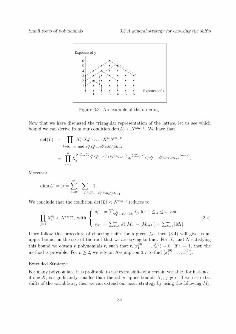
Small roots of polynomials 3.3 A general strategy for choosing the shifts
1 2 3 4 5 6Exponent of x
123456
Exponent of y
Figure 3.3: An example of the ordering
Now that we have discussed the triangular representation of the lattice, let us see whichbound we can derive from our condition det(L) < Nmω−ε. We have that
det(L) =∏
k=0,...,m and xi11 x
i22 ·...·xiv
v ∈Mk\Mk+1
X i11 X i2
2 · . . . ·X ivv Nm−k
=v∏
j=1
X
Pmk=0
Px
i11 x
i22 ·...·xiv
v ∈Mk\Mk+1ij
j N
Pmk=0
Px
i11 x
i22 ·...·xiv
v ∈Mk\Mk+1(m−k)
.
Moreover,
dim(L) = ω =m∑
k=0
∑
xi11 x
i22 ·...·xiv
v ∈Mk\Mk+1
1.
We conclude that the condition det(L) < Nmω−ε reduces to
v∏j=1
Xsj
j < N sN−ε, with
sj =∑
xi11 ...xiv
v ∈M0ij, for 1 ≤ j ≤ v, and
sN =∑m
k=0 k(|Mk| − |Mk+1|) =∑m
k=1 |Mk|.(3.4)
If we follow this procedure of choosing shifts for a given fN , then (3.4) will give us anupper bound on the size of the root that we are trying to find. For Xj and N satisfying
this bound we obtain v polynomials ri such that ri(x(0)1 , . . . , x
(0)v ) = 0. If v = 1, then the
method is provable. For v ≥ 2, we rely on Assumption 3.7 to find (x(0)1 , . . . , x
(0)v ).
Extended Strategy:
For many polynomials, it is profitable to use extra shifts of a certain variable (for instance,if one Xi is significantly smaller than the other upper bounds Xj, j 6= i. If we use extrashifts of the variable x1, then we can extend our basic strategy by using the following Mk.
34

Small roots of polynomials 3.3 A general strategy for choosing the shifts
Mk :=⋃
0≤j≤t
{xi1+j1 xi2
2 · . . . · xivv | xi1
1 xi22 · . . . · xiv
v is a monomial of fmN
andxi1
1 xi22 · . . . · xiv
v
lkis a monomial of fm−k
N }.
Moreover, extra shifts of several variables, or combined shifts should be considered to ob-tain an optimal bound. The number of extra shifts can be described using a parameter tthat can be optimized. Using this new definition of Mk, the rest of the strategy conformsto the basic strategy as described before. Let us now give some examples, and show howthe known results on small modular roots from [6, 10, 16] are all special cases of our basicor extended strategy.
Examples:
Here, we show that the known results of Boneh and Durfee, Blomer and May, and Copper-smith [10, 6, 16] in this field are special cases of our strategy. Although they were originallydescribed in different ways, their results can also be obtained if one follows the basic orextended strategy described in this section.
‘Boneh/Durfee attack’ [10]:
Recall that in the attack by Boneh and Durfee [10], the goal was to find the small root(d, p + q − 1) of the polynomial fe(x, y) = 1 + x(N − y) modulo e.
Let us discuss in general how small a root (x0, y0) of a polynomial
fN(x, y) = a0 + a1x + a2xy
modulo some N should be such that it can be found by a Coppersmith method. The knownbound that the upper bounds X and Y have to satisfy is
X2+3τY 1+3τ+3τ2
< N1+3τ−ε.
Here and in the following attack bounds, τ > 0 is always a parameter that can be optimizedafter plugging in the values for X, Y and N .
The bound can be obtained by following our extended strategy with extra shifts of y.As we described above, the extended strategy then prescribes
Mk :=⋃
0≤j≤t
{xi1yi2+j
∣∣∣∣xi1yi2 monomial of fmN and
xi1yi2
lkmonomial of fm−k
N }, for l = xy.
Figures 3.4 and 3.5 show the monomials of fmN (which would be used if one would only
apply the basic strategy) and the new sets Mk when including extra y-shifts. One cancheck that a correct description of the sets Mk is
xi1yi2 ∈ Mk ⇔ i1 = k, . . . , m and i2 = k, . . . , i1 + t,
for some t = τm (in the figure, t = 2 is shown).
35

Small roots of polynomials 3.3 A general strategy for choosing the shifts
x2
x2y
x2y2
Mm ® xmym
1 x xm
xmy
xmy2
xy
M0�M1
M1�M2
M2�M3
...
Figure 3.4: Shape of fmN
xmym+1
xmym+2
y
y2 xy2
xy3x2y3
x2y4
M0�M1
M1�M2
M2�M3
�Mm
...
Figure 3.5: Extra y-shifts
Substituting this definition of Mk in the bound of (3.4) leads to
X16(m3(2+3τ)+m2(6+3τ)+m·4)Y
16(m3(1+3τ+3τ2)+m2(3+6τ+3τ2)+m(2+3τ))
< N16(m3(1+3τ)+m2(3+3τ)+m·2)−ε.
If we let all terms of order o(m3) contribute to ε, then we see that for m →∞, this boundreduces to
X2+3τY 1+3τ+3τ2
< N1+3τ−ε.
To illustrate the example, we show how the matrix describing the lattice L looks for m = 2,t = 1. Since the Boneh/Durfee-attack is about finding a root modulo e, we will use theterminology of fe from here on instead of fN .
e2
e2Xe2X2
e2Yea′0 ea′1X eXY
ea′0X ea′1X2 eX2Y
ea′0Y ea′1XY eXY 2
a′20 2a′0a′1X a′21 X2 2a′0XY 2a′1X
2Y X2Y 2
a′20 Y 2a′0a′1XY 2a′0XY 2 a′21 X2Y 2a′1X
2Y 2 X2Y 3
Figure 3.6: Example of a Boneh/Durfee-lattice: m = 2, t = 1
The columns of the matrix correspond to the monomials 1, x, x2, y (of M0\M1), xy, x2y, xy2
(of M1\M2) and x2y2, x2y3 (of M2) respectively. The rows represent the shifts gi1i2(x, y) :=xi1yi2(f ′e(x, y))kem−k, where f ′e(x, y) = a−1
2 fe(x, y) = a′0 + a′1x + xy.
36

Small roots of polynomials 3.3 A general strategy for choosing the shifts
In the case of the Boneh/Durfee-attack on RSA-Small-d, we know that the root (x0, y0)
we are looking for has upper bounds X = Nβ and Y = 3N12 . Since we put all terms that
do not depend on N in our error term ε, we see that
β(2 + 3τ) +1
2(1 + 3τ + 3τ 2) < 1 · (1 + 3τ)
is the asymptotical bound of the attack. This reduces to
3τ 2 + 3τ(2β − 1) + (4β − 1) < 0.
The left hand side polynomial has its maximum for τ = 12− β. Substituting this value, we
obtain
−3β2 + 7β − 7
4< 0,
which reduces to β < 76− 1
3
√7 ≈ 0.284.
In [10], Boneh and Durfee improve this bound a little more to β < 1 − 12
√2 ≈ 0.292.
They improve the bound by looking at sublattices of the lattice described before. Acomplication with this technique is that the sublattices no longer have full rank, whichmakes the analysis harder. We go into more detail about sublattices in Section 7.2.
For completeness, Boneh/Durfee’s result is stated in the following theorem.
Theorem 3.10 (Boneh/Durfee, [10])Under Assumption 3.7, for every ε > 0, there exists n0 such that for every n > n0, thefollowing holds: Let N = pq be an n-bit RSA modulus, and p, q primes of bitsize 1
2n.
Moreover, let d < N0.292−ε. Given N , and e such that ed = 1 mod φ(N), one can recoverd in time polynomial in n.
‘Blomer/May attack’ [6]:
In Section 4.2, we discuss the known partial key exposure attacks on RSA, among whichare attacks by Blomer and May that use the following polynomial:
fN(x, y, z) = a0 + a1x + a2y + a3yz.
Here, we sketch how the known bound for this polynomial,
X1+4τY 2+4τZ1+4τ+6τ2
< N1+4τ−ε,
can be obtained by following our extended strategy with extra shifts of z.Suppose we choose l = x as leading monomial. Then the set Mk can be described as
Mk :=⋃
0≤j≤t{xi1yi2zi3+j |xi1yi2zi3 monomial of fmN
and xi1yi2zi3
lkmonomial of fm−k
N }.
37
Small roots of polynomials 3.3 A general strategy for choosing the shifts
We find that
xi1yi2zi3 ∈ Mk ⇔ i1 = k, . . . , m ; i2 = 0, . . . ,m− i1 ; i3 = 0, . . . , i2 + t,
for some t = τm. Substituting this new definition of Mk in the bound (3.4) will result inBlomer/May’s bound.
Generalized Rectangles and Generalized Lower Triangles [16]:
Now that we have used our extended strategy twice to obtain the known bounds ofBoneh/Durfee and Blomer/May, we also mention two generalizations of known resultsthat can be derived using only the basic strategy.
Suppose fN(x1, . . . , xv) is a polynomial with the shape of a generalized rectangle, thatis, the degree of xi is λiD. Then the bound (heuristically for v ≥ 2) for which a root
(x(0)1 , . . . , x
(0)v ) of fN modulo N can be found, is given by
Xλ11 · . . . ·Xλv
v < N2
(v+1)D−ε.
This bound is a generalization of Coppersmith’s bound X < N1D [16] and the heuristic
extension XY < N2
3D . Nguyen and Stern [59] already mentioned the bound Xλ1Y λ2 <
N2
3D , for the bivariate case.The general result can be obtained by following the basic strategy, with
l = xλ1D1 · xλ2D
2 · . . . · xλvDv ,
and
xi11 xi2
2 · . . . · xivv ∈ Mk ⇔ ij = λjDk, . . . , λjDm (j = 1, . . . , v).
Suppose fN(x1, . . . , xv) is a polynomial with the shape of a generalized lower triangle,that is, its monomials are xi1
1 · . . . · xivv for
0 ≤ i1 ≤ λ1D, 0 ≤ i2 ≤ λ2D − λ2
λ1
i1, . . . , 0 ≤ iv ≤ λvD −v−1∑r=1
λvD
λr
ir.
Then the bound (heuristically for v ≥ 2) is given by
Xλ11 · . . . ·Xλv
v < N1D−ε.
The known special cases are those for fN(x) or fN(x, y) with total degree D (in other
words, λj = 1). Both X < N1D and XY < N
1D appeared in [16].
The general bound can be easily derived by following the basic strategy with l = xλ1D1
and
xi11 xi2
2 · . . . · xivv ∈ Mk ⇔ i1 = λ1Dk, . . . , λ1Dm ;
ij = 0, . . . , λjDm−∑j−1r=1
λj
λrir (j = 2, . . . , v).
38

Small roots of polynomials 3.3 A general strategy for choosing the shifts
x2
x2yxy
y1
x
zyzxz
x2zxyz
x2yz
Figure 3.7: Generalized Rectangle
x2 y1
x
z
Figure 3.8: Generalized Lower Triangle
3.3.2 Small integer roots
Suppose we want to find a small integer root (x(0)1 , . . . , x
(0)v ) of an irreducible polynomial f .
We know that the root is small in the sense that |x(0)j | < Xj, for j = 1, . . . , v.
The goal in this section is to choose the shift polynomials
gi1...iv := xi11 · . . . · xiv
v f(x1, . . . , xv) · R
WXi11 ·...·Xiv
v
and
g′i1...iv := xi11 · . . . · xiv
v R,
that define the lattice L in such a way that they produce a good bound
det(L) < 2−ω(ω−1)
4 ·(
1√ω
)ω+2−v
·Rω+2−v. (3.5)
To obtain a simple, asymptotic bound, we again introduce an error term ε for all theterms that do not depend on N . This means that instead of checking (3.5), we simply usedet(L) < Rω+2−v−ε. If the number of variables v is taken to be constant, we can furthersimplify the condition to
det(L) < Rω−ε. (3.6)
Analogously to the modular case, we fix an integer m depending on ε. We call dj themaximal degree of xj in f , and W the maximal absolute coefficient of f(x1X1, . . . , xvXv).
Moreover, we define R = W∏n
j=1 Xdj(m−1)j . To work with a polynomial with constant
term 1, we define f ′ = a−10 f mod R, where a0 is the constant term of f . This means that
we should have a0 6= 0 and gcd(a0, R) = 1. The latter is easy to achieve, analogous to[18, Appendix A], since any Xj with gcd(a0, Xj) 6= 1 can be changed into an X ′
j such thatXj < X ′
j < 2Xj and gcd(a0, X′j) = 1. The same holds for W .
39

Small roots of polynomials 3.3 A general strategy for choosing the shifts
Let us now consider the case a0 = 0. In [18, Appendix A], Coron discussed this casefor bivariate polynomials, and showed a simple way to transfer a polynomial f with zeroconstant term into a polynomial f ∗ with nonzero constant term.
A general way to do this for multivariate polynomials would be the following. First,we find a nonzero integer vector (y1, . . . , yv) such that f(y1, . . . , yv) 6= 0. This can beconstructed in polynomial time since there are only polynomially many roots within thegiven bounds. Then we define f ∗(x1, . . . , xv) := f(x1 + y1, . . . , xv + yv), and look for rootsof f ∗. Since f ∗(0, . . . , 0) = f(y1, . . . , yv), f ∗ has a nonzero constant term.
We would like to point out that the switch to f ∗ will affect the set of monomials, andnew monomials may appear in f ∗ that were not in f . This may affect the analysis andlead to a different Coppersmith-type bound. This issue already appears with bivariatepolynomials, but it did not affect Coron’s analysis since in his case the set of monomialsstayed the same. From now on we will assume that a0 6= 0. In the unfortunate casethat a0 = 0 and switching to f ∗ leads to a different monomial set, we suggest to useCoppersmith’s original method1 (as explained in Section 5.3.3).
Let us now describe our strategy for choosing the shifts in the case of integer roots. Asbefore, we start with the basic strategy, that we extend later to obtain the full strategy.
Basic Strategy:
We define S and M as the sets of monomials of fm−1 and fm respectively. We denote bylj the largest exponent of xj that appears in the monomials of S, i.e. lj = dj(m− 1).
Next, we define the following shift polynomials
gi1...iv : xi11 xi2
2 · . . . · xivv f ′(x1, . . . , xv)
∏nj=1 X
lj−ijj , for xi1
1 xi22 · . . . · xiv
v ∈ S,
g′i1...iv : xi11 xi2
2 · . . . · xivv R, for xi1
1 xi22 · . . . · xiv
v ∈ M\S.
All gi1...iv and g′i1...iv have the root (x(0)1 , . . . , x
(0)v ) modulo R. The coefficient vectors of
gi1...iv(x1X1, . . . xvXv) and g′i1...iv(x1X1, . . . xvXv) form a lattice basis of a lattice L.
Using the following ordering of the monomials of S, we can order the basis matrix such
that it is upper triangular. We say that xi11 · . . . · xiv
v < xi′11 · . . . · xi′v
v if∑
ij <∑
i′j. If∑ij =
∑i′j, then we use the lexicographical ordering.
The diagonal elements of the rows of g are those corresponding to the constant term
in f ′. Therefore, the diagonal entries of the matrix are∏n
j=1 Xdj(m−1)j for the polynomials g
and W∏n
j=1 Xdj(m−1)+ijj for the polynomials g′.
For constant v, we know that the determinant condition det(L) < Rω−ε ensures thatthe v − 1 smallest vectors in an LLL reduced basis of L correspond to v − 1 polynomialsri(x1, . . . xv) with ri(x
(0)1 , . . . , x
(0)v ) = 0.
1One could also use Coron’s new method, as presented at Crypto’07 [19].
40

Small roots of polynomials 3.3 A general strategy for choosing the shifts
We find that the condition det(L) < Rω−ε reduces to
v∏j=1
Xsj
j < W sW−ε, for sj =∑
xi11 ...xiv
v ∈M\S
ij , and sW = |S|. (3.7)
So if the bound (3.7) holds, we obtain v− 1 polynomials ri such that ri(x(0)1 , . . . , x
(0)v ) = 0.
By Theorem 3.9, these polynomials are independent of f . So, under Assumption 3.7, theresultant computations of f and ri (for i = 1, . . . , v − 1) will reveal the root.
Extended Strategy:
As in the modular case, our strategy is not finished before exploring the possibilities ofextra shifts of a certain variable (or more variables). Suppose we use extra shifts of thevariable x1. Then, instead of S = {monomials of fm−1} and M = {monomials of fm}, weuse
S =⋃
0≤j≤t
{xi1+j1 xi2
2 · . . . · xivv | xi1
1 xi22 · . . . · xiv
v is a monomial of fm−1},
M = {monomials of xi11 xi2
2 · . . . · xivv · f | xi1
1 xi22 · . . . · xiv
v ∈ S}.With the new definitions, the rest of the strategy conforms to the basic strategy, except
for the value of R. It is necessary to change R = W∏v
j=1 Xdj(m−1)j into R = W
∏vj=1 X
ljj ,
where lj is the largest exponent of xj that appears in the monomials of S.
Examples:
Here, we collect the known results by Blomer and May and Coppersmith [7, 16] for poly-nomials fN with a small integer root. These known results are again special cases of ourextended or basic strategy. As our strategy for finding small integer roots is a generali-zation of the technique described in [7] to more variables, the first claim is not surprising.The examples we give in this section are very brief, since we will treat new polynomialsfor new attacks in more detail throughout this thesis.
‘Blomer/May, upper triangle’ [7]:
In [7], Blomer and May describe an alternative method to obtain the attack that Boneh,Durfee, and Howgrave-Graham published on Takagi’s RSA variant [13]. For N = prq, andan approximation p of p, one could try to find the root of the polynomial
f(x, y) = (p + x)ry −N.
This is an example of what Blomer and May call a polynomial with the shape of an uppertriangle. In general, we deal with a polynomial f(x, y) with xi1yi2 for i2 = 0, . . . , D andi1 = 0, . . . , λi2, for instance f(x, y) = a0 + a1y + a2xy + a3x
2y (where D = 1 and λ = 2).The known bound is
X(λ+τ)2Y 2(λ+τ) < W1D
(λ+2τ)−ε.
41

Small roots of polynomials 3.3 A general strategy for choosing the shifts
Figures 3.9 and 3.10 show the monomials of fm (which would be used if one would followthe basic strategy) and shapes of S and M if one uses extra shifts of x.
yDm
yD Hm-1L
1
yD xΛ DyD
xΛ D Hm-1LyD Hm-1L
xΛ DmyDm
M�S
S
Figure 3.9: Shape of fm
xΛD+tyD
xΛDm+tyDm
xt
¯
M�S
S
Figure 3.10: Extra x-shifts
One can check that the new definitions of S and M are
xi1yi2 ∈ S ⇔ i2 = 0, . . . , D(m− 1) ; i1 = 0, . . . , λi2 + t.
xi1yi2 ∈ M ⇔ i2 = 0, . . . , Dm ; i1 = 0, . . . , λi2 + t.
for some t = τDm.Substituting this in inequality (3.7) will lead to the bound as given above.
‘Blomer/May, extended rectangle’ [7]:
Another type of polynomial that Blomer and May study in their paper about integerroots of polynomials, is the polynomial with the shape of an extended rectangle. That is,f(x, y) with xi1yi2 for i2 = 0, . . . , D, i1 = 0, . . . , γD + λ(D − i2), for instance f(x, y) =a0 + a1x + a2x
2 + a3x3 + a4y + a5xy (where D = 1 and γ = 1 and λ = 2). The known
bound is
Xλ2+3γλ+2τλ+4τγ+τ2+3γ2
Y λ+3γ+2τ < W1D
(λ+2γ+2τ)−ε.
Besides the shifts of the basic strategy (Figure 3.11), we use extra x-shifts (Figure 3.12)and work with
xi1yi2 ∈ S ⇔ i2 = 0, . . . , D(m− 1) ;i1 = 0, . . . , γD(m− 1) + λ(D(m− 1)− i2) + t.
xi1yi2 ∈ M ⇔ i2 = 0, . . . , Dm ;i1 = 0, . . . , γDm + λ(Dm− i2) + t.
for some t = τDm. This leads to the bound as stated above.
42

Small roots of polynomials 3.3 A general strategy for choosing the shifts
xΓDmyDm
xHΓ+ΛLDm
yDm
1
S
M�S
Figure 3.11: Shape of fm
xΓDm+tyDm
xHΓ+ΛLDm+t
S
M�S
Figure 3.12: Extra x-shifts
Generalized Rectangles and Generalized Lower Triangles [16]
As in the modular case, we mention two generalizations of known results that can bederived using only the basic strategy.
Suppose f(x1, . . . , xv) is a polynomial with the shape of a generalized rectangle, that is,the degree of xi is λiD. Then the bound (heuristically for v ≥ 3) is
Xλ11 · . . . ·Xλv
v < W2
(v+1)D−ε.
The first special case of this situation was again analyzed by Coppersmith in [16], finding
the bound XY < W2
3D for polynomials f(x, y) with degree D per variable. In [7], Blomerand May generalized this for bivariate polynomials to the case of rectangles instead ofsquares. Our result is a generalization of the one described in [7] to polynomials with anynumber of variables.
The bound can easily be derived by following the basic strategy, with
xi11 xi2
2 · . . . · xivv ∈ S ⇔ ij = 0, . . . , λjD(m− 1) (j = 1, . . . , v)
xi11 xi2
2 · . . . · xivv ∈ M ⇔ ij = 0, . . . , λjDm (j = 1, . . . , v)
Suppose f(x1, . . . , xv) is a polynomial with the shape of a generalized lower triangle,that is, its monomial are xi1
1 · . . . · xivv for
0 ≤ i1 ≤ λ1D, 0 ≤ i2 ≤ λ2D − λ2
λ1
i1, . . . , 0 ≤ iv ≤ λvD −v−1∑r=1
λv
λr
ir.
Then the bound (heuristically for v ≥ 3) is
Xλ11 · . . . ·Xλv
v < W1D−ε.
43

Small roots of polynomials 3.4 Tabular overview
The first known example is the polynomial f(x, y) with total degree D, analyzed by Copper-
smith [16]. He showed that the bound for this situation is XY < W1D . The generalization
to lower triangles with unequal sides was again made by Blomer and May [7], for a bi-variate polynomial f(x, y) such that the monomials xi1yi2 appear for 0 ≤ i1 ≤ D and0 ≤ i2 ≤ λD − i1. Our result is an extension of their two-dimensional case.
To obtain the general bound, one can use
xi11 xi2
2 · . . . · xivv ∈ S ⇔ ij = 0, . . . , λjD(m− 1)−∑j−1
r=1λj
λrir for j = 1, . . . , v,
xi11 xi2
2 · . . . · xivv ∈ M ⇔ ij = 0, . . . , λjDm−∑j−1
r=1λj
λrir for j = 1, . . . , v.
3.4 Tabular overview
In the following tables, we give an overview of all results concerning bounds for findingroots with Coppersmith methods. The first table includes the results for finding smallmodular roots, the second for finding small integer roots. In the second table, we haveadded some new results, corresponding to attacks that will be explained in detail in thefollowing chapters.
Monomials of fN Bound Reference
1, x, xy X2+3τY 1+3τ+3τ2< N1+3τ−ε Boneh/Durfee [10]
1, x, y, yz X1+4τY 2+4τZ1+4τ+6τ2< N1+4τ−ε Blomer/May [6]
generalized Xλ11 · . . . ·Xλv
v < N2
(v+1)D−ε generalization of
rectangle Coppersmith [16]
generalized Xλ11 · . . . ·Xλv
v < N1D−ε generalization of
lower triangle Coppersmith [16]
Table 3.1: Bounds for finding small modular roots of polynomials
44

Small roots of polynomials 3.4 Tabular overview
Monomials Bound Referenceof f
upper triangle X(λ+τ)2Y 2(λ+τ) < W1D
(λ+2τ)−ε Blomer/May [7]
extended Xλ2+3γλ+2τλ+4τγ+τ2+3γ2Y λ+3γ+2τ < W
1D
(λ+2γ+2τ)−ε Blomer/May [7]rectangle
generalized Xλ11 · . . . ·Xλv
v < W2
(v+1)D−ε generalization of
rectangle Coppersmith [16]
generalized Xλ11 · . . . ·Xλv
v < W1D−ε generalization of
lower triangle Coppersmith [16]
1, x, y, yz X1+3τY 2+3τZ1+3τ+3τ2< W 1+3τ−ε Section 4.4.2
1, x, y, z, yz X2+3τY 3+6τ+3τ2Z3+3τ < W 2+3τ−ε Section 4.4.2
1, x1, x2, x3, x4, (X1X2)5+20τ+27τ2+12τ3(X3X4)5+20τ+18τ2
< W 3+12τ+12τ2−ε Section 5.3.1x1x2, x1x4,x2x3, x3x4
1, x, x2, y, z, X7+9τ+3τ2(Y Z)5+ 9
2τ < W 3+3τ−ε Section 5.4.1
xy, xz, yz
Table 3.2: Bounds for finding small integer roots of polynomials
45

Small roots of polynomials 3.5 Complexity of attacks using Coppersmith’s method
3.5 Complexity of attacks using Coppersmith’s method
In the next chapters we will show many attacks on RSA variants that use Coppersmithmethods. For those attacks, we claim that the factorization of the RSA modulus N canbe found in time polynomial in n, the bitsize of N . Therefore, we conclude this chapter bycommenting on the complexity of Coppersmith methods.
The running time of a Coppersmith method is dominated by the lattice basis reduc-tion. A reduction using the algorithm of Nguyen and Stehle [58] can be performed in timeO(ω5(ω+A)A), where A is the maximal bitsize of an entry in the lattice L of dimension ω.Our lattice dimension ω depends on ε only, whereas the bitsize of the entries of the latticein our attacks will be bounded by a polynomial in n, the bitsize of N . Therefore, theconstruction of r1, . . . , rv can be done in time polynomial in n. Moreover, the polyno-mials r1, . . . , rv have a fixed degree that only depends on ε, and coefficients with bitsizepolynomial in n.
If r1(x1, . . . , xv), r2(x1, . . . , xv) are two polynomials with degx1(r1) = d1, degx1
(r2) = d2,then computing a resultant Resx1(r1, r2) consists of computing a determinant of a matrixof size (d1 +d2)× (d1 +d2). The total degree of the resultant (a polynomial in the variables(x2, . . . , xv)) is polynomial in the total degree of r1 and r2. Equivalently, the size of thecoefficients of the resultant is polynomial in the original coefficient sizes. To extract theroot, we need to repeat this process of computing resultants a fixed number of times. Everytime, computing the determinant of a matrix of size D×D can be done in a running timeof order D3. For details on resultant computations, we refer to [21, Chapter 3].
In Section 5.3 we use Grobner bases as an alternative to resultants in the process offinding a common root from a set of polynomials. Computing a Grobner basis can bedone using the F4 algorithm [26] implemented in Magma. The complexity of computinga Grobner basis for a system of equations with a finite number of solutions is polynomialin Dv, where D is the maximal degree of the input polynomials (see for instance [29,Section 10.5]). However, in our attacks, both D and v will be fixed. To prevent thecoefficients in the Grobner basis from exploding, we could compute the Grobner basis overZp′ , where p′ is a prime larger than the RSA modulus N .
Hence, for a fixed ε, and a fixed number of variables, using Coppersmith’s method tofind a root can be done in polynomial time. However, note that in both the reduction phaseand in the resultants/Grobner phase, we can run into practical limitations. Although alattice basis can be reduced in polynomial time, it could be that the reduction of a 300-dimensional lattice takes days or weeks on a computer. The same holds for the computationof resultants and Grobner bases (especially for a larger number of variables). That is whyexperiments are needed to show the practical implications of theoretical attacks usingCoppersmith methods.
46

4Partial key exposure attacks on RSA
In this chapter, we discuss the known attacks on RSA-Small-e where a part of the bits of dis known to an attacker. Moreover, we discuss some new partial key exposure attacks onRSA-Small-d and RSA-Small-e.
Section 4.3 is based on [36], which is joint work with Benne de Weger. Section 4.4 isbased on [25], a joint paper with Matthias Ernst, Alexander May, and Benne de Weger.
4.1 Introduction
The concept of partial key exposure attacks on RSA was introduced in 1997 by Boneh,Durfee and Frankel [12], and deals with the situation where an attacker has obtained somebits of the private exponent d. The main question is:
How much information on the bits of d is needed such that an attacker can efficientlyreconstruct d, thereby breaking the RSA instance?
The motivation for exploring partial key exposure attacks comes from side channelattacks such as power analysis, timing attacks, etc. Using a side channel, an attacker canexpose a part of d, generally some MSBs (most significant bits) or LSBs (least significantbits). To see why an attacker usually gets either MSBs or LSBs of the secret exponent, werefer to [53].
In all subsequent papers about partial key exposure attacks on RSA, the assumptionis made (besides knowledge of MSBs/LSBs of d) that one of the exponents e, d (or, inRSA-CRT variants, e or dp and dq) is chosen to be small. This means that either e or dis at least significantly smaller than the modulus N . In Section 4.2 we will discuss thesepartial key exposure attacks on RSA-Small-e. The known partial key exposure attacks onRSA-CRT variants will be discussed in Chapter 5.
In Section 4.3 we discuss a simple but very efficient partial key exposure attack onRSA-Small-d using a 2-dimensional lattice. As mentioned before, RSA-Small-d is es-pecially useful for signing operations on constrained devices such as smartcards. Onecould choose a private exponent d that is large enough to counter the attacks by Wienerand Boneh/Durfee [75, 10]. However, since side channel attacks are often mounted on
47

Partial key exposure attacks on RSA 4.2 Known attacks
smartcard-settings, exploring the possibilities of partial key exposure attacks on RSA-Small-d is very important. The attack we discuss in Section 4.3 is a generalization of theattacks by Wiener [75] and Verheul/van Tilborg [72] to partial key exposure attacks.
In Section 4.4 we discuss new partial key exposure attacks on RSA-Small-e and RSA-Small-d. In fact, we show that whenever one of the exponents e, d is chosen significantlysmaller than N , a partial key exposure attack exists.
4.2 Known attacks
Although Boneh, Durfee, and Frankel [12] introduced attacks that use partial knowledge ofthe secret exponent d, we shall start with a result of Coppersmith that the attacks in [12]are based on.
Theorem 4.1 (Coppersmith, [16])Let N = pq be an n-bit RSA modulus, with p and q primes of bitsize 1
2n. Suppose that either
the high-order 14n bits of p or the low-order 1
4n bits of p are known. Then the factorization
of N can be found in time polynomial in n.
Proof.As Coppersmith showed in [16], this result can easily be derived from one of Coppersmith’sbounds that we mentioned in Section 3.3.2. In [16], Coppersmith derives the bound
XY < W2
3D−ε
for polynomials f(x, y) with degree per variable D. Suppose that an attacker knows an
MSB part of p of size at least N12−δ. That means that he knows an approximation p of p
such that the unknown part p0 = p− p satisfies |p0| < N δ. Additionally, he can also derivean approximation q of q such that |q0| = |q − q| < N δ. The polynomial
f(x, y) = (p + x)(q + y)−N
has a root (x0, y0) = (p0, q0). Since f is a polynomial where the degree per variable is 1,
it holds that if XY < W23−ε is satisfied, then the unknown p0 and q0 can be found. Here,
X = Y = N δ and W = max{qX, pY, XY, |N − pq|} = N12+δ. Hence, the asymptotic bound
is
2δ <2
3
(1
2+ δ
)
which leads to δ < 14. The result for known LSBs of p can be derived in a similar way.
2
The first partial key exposure attack on RSA-Small-e, by Boneh, Durfee, and Frankel, issummarized in the following theorem.
48
Partial key exposure attacks on RSA 4.2 Known attacks
Theorem 4.2 (Boneh/Durfee/Frankel (LSBs), [12])Let N = pq ≡ 3 mod 4 be an n-bit RSA modulus, and p, q primes of bitsize 1
2n. Let e,
d satisfy ed ≡ 1 mod φ(N) with bitsize(e) = αn and bitsize(d) = n, for some α ∈ (0, 14).
Suppose that an LSB part of d is known of at least 14n bits. Then the factorization of N
can be found in time polynomial in n and e.
Proof sketch.For a formal proof, we refer to [11]. However, we will sketch how this attack uses Copper-smith’s theorem (Theorem 4.1). Suppose d0 ≡ d mod 2B is the known LSB part of d.Then the RSA key equation ed = 1 + k(N + 1− (p + q)) implies that
ed0 ≡ 1 + k(N + 1− s) mod 2B, for s = p + q.
If all possibilities for k ∈ {1, . . . , e} are tried then in one of these trials s0 ≡ p+ q mod 2B
can be found. Next, one tries to solve the equation
p2 − s0p + N ≡ 0 mod 2B,
of which p0 ≡ p mod 2B is a solution. A solution x = (p− s0
2) modulo 2B of
x2 ≡(s0
2
)2
−N mod 2B,
can easily be found if the right hand side is congruent to 1 modulo 8 (see [63, p.184] for adescription of the method). Now,
(s0
2
)2
−N ≡ (p− q)2
4mod 2B
and N ≡ 3 mod 4 ensures that the right hand side is congruent to 1 modulo 8. Hence,p0 ≡ p mod 2
n4 can be found. With Theorem 4.1, this reveals the factorization of N .
2
Since RSA-Small-e is a popular variant, the above attack for which only a quarter of theLSBs of d are necessary is very serious. Steinfeld and Zheng [68] discovered that the aboveattack works less well if p−q is a multiple of a large power of 2. Suppose that p−q = 2A ·yfor some odd integer y. Then
(s0
2
)2
−N ≡ (p− q)2
4≡ 22A−2y2 mod 2B.
Therefore,( x
2A−1
)2
≡ y2 mod 2B−2A+2.
Hence, if y2 ≡ 1 mod 8, then one can obtain only p mod 2B−A+1 instead of p mod 2B.Therefore, Steinfeld and Zheng [68] propose to choose p and q such that they share a
number of LSBs, in order to diminish the power of the attack in [12]. Whether or not thisspecific design criterion for p and q gives rise to other attacks is still an open question.
49

Partial key exposure attacks on RSA 4.2 Known attacks
The known attacks from [12] on RSA-Small-e with known MSBs of d are summarized inthe following theorem.
Theorem 4.3 (Boneh/Durfee/Frankel (MSBs), [12])Let N = pq be an n-bit RSA modulus, and p, q primes of bitsize 1
2n. Let e, d satisfy ed ≡ 1
mod φ(N) with bitsize(e) = αn and bitsize(d) = n, for some α ∈ (0, 12). Suppose that an
MSB part of d is known of size at least N1−δ. Then the following statements are true.
1. If e is prime and α ∈ (14, 1
2), then the factorization of N can be found in time
polynomial in n if δ < 1− α.
2. If e is a product of r distinct (known) factors and α ∈ (14, 1
2), then the factorization
of N can be found in time polynomial in n and 2r if δ < 1− α.
3. If the factorization of e is unknown and α ∈ (0, 12), then the factorization of N can
be found in time polynomial in n and Nd
if δ < α.
4. If the factorization of e is unknown and α ∈ (0, 12), then the factorization of N can
be found in time polynomial in n, Nd, and
√N
p−q, if δ < 1
4.
For the proofs, we refer to [12]. Most of the proofs, like the one for Theorem 4.2, usethe information that is given to find either MSBs or LSBs of p, after which Theorem 4.1is applied. Another fact that is used in some of the proofs is that for e < N
12 , the value of
k := ed−1φ(N)
is known up to some constant error if as many MSBs of d as the bitsize of e aregiven. Since this result influences our new attacks, we will discuss it briefly.
Theorem 4.4 (Boneh/Durfee/Frankel, [12])Let N = pq be an n-bit RSA modulus, and p, q primes of bitsize 1
2n. Let e, d satisfy ed ≡ 1
mod φ(N) with bitsize(e) = αn and bitsize(d) = n, for some α ∈ (0, 12). Suppose that an
MSB part of d is known of size at least Nα. Then an approximation k of k = ed−1φ(N)
can be
computed such that the difference between k and k is bounded by a constant.
Proof.Suppose d = d + d0, where d is a known approximation of d and d0 is the unknown LSB
part of d of size N δ for some δ < 1− α. Then, for k = ed−1N
,
∣∣∣k − k∣∣∣ =
∣∣∣∣∣e(d + d0)− 1
φ(N)− ed− 1
N
∣∣∣∣∣ =
∣∣∣∣∣(ed− 1)(N − φ(N)) + ed0N
Nφ(N)
∣∣∣∣∣
<e
φ(N)
∣∣∣∣∣d · 3N 1
2
N+ d0
∣∣∣∣∣ <Nα
12N
(3N
12 + N δ
)= 6Nα− 1
2 + 2Nα+δ−1 < 8.
2
50

Partial key exposure attacks on RSA 4.2 Known attacks
Boneh, Durfee and Frankel posed the open question whether or not there exist partial keyexposure attacks for e > N
12 . This question was answered affirmatively by Blomer and
May, who showed other partial key exposure attacks. Their best results are summarizedin the following theorems.
Theorem 4.5 (Blomer/May (LSBs), [6])Under Assumption 3.7, for every ε > 0, there exists an integer n0 such that for everyn > n0 the following holds: Let N = pq be an n-bit RSA modulus, and p, q primes ofbitsize 1
2n. Let e, d satisfy ed ≡ 1 mod φ(N) with bitsize(e) = αn and bitsize(d) = n,
for some α ∈ (0, 78). Suppose that an LSB part of d is known of size at least N1−δ, with
δ ∈ (0, 1), and
δ <5
6− 1
3
√1 + 6α− ε.
Then N can be factored in time polynomial in n.
Proof.One can write d as d = d0 + x2(1−δ)n, where x is the unknown MSB part of d of size N δ.Hence,
e(d0 + x2(1−δ)n) = 1 + k(N + 1− (p + q)).
It follows that
fe2(1−δ)n(y, z) = ed0 − 1− y(N + 1− z)
has a small root (y0, z0) = (k, p + q) modulo e2(1−δ)n.From the “Boneh/Durfee” example in Section 3.3.1, one can see that for roots of a
polynomial modulo e2(1−δ)n, with monomials 1, y, yz, for some τ ≥ 0 that can be optimizedlater, the following bound holds:
X2+3τY 1+3τ+3τ2
< (e2(1−δ)n)1+3τ−ε.
Substituting Y = Nα and Z = N12 leads to the asymptotical bound
α(2 + 3τ) +1
2(1 + 3τ + 3τ 2) < (α + 1− δ)(1 + 3τ), or
3τ 2 + 3τ(2δ − 1) + (2α + 2δ − 1) < 0.
The optimal τ = 12− δ gives
δ <5
6− 1
3
√1 + 6α.
2
51

Partial key exposure attacks on RSA 4.2 Known attacks
Theorem 4.6 (Blomer/May (MSBs), [6])Under Assumption 3.7, for every ε > 0, there exists an integer n0 such that for everyn > n0 the following holds: Let N = pq be an n-bit RSA modulus, and p, q primes ofbitsize 1
2n. Let e, d satisfy ed ≡ 1 mod φ(N) with bitsize(e) = αn and bitsize(d) = n, for
some α ∈ (12,√
6−12
). Suppose that an MSB part of d is known of size at least N1−δ, withδ ∈ (0, 1), and
δ <1
8(5− 2α−
√36α2 + 12α− 15)− ε.
Then N can be factored in time polynomial in n.
Proof.One can write d as d = d+d0, where d0 is the unknown LSB part of d of size N δ. Knowledgeof MSBs of d also leads to knowledge of MSBs of k, since
k =ed− 1
N + 1
is a good approximation of k. Analogous to the proof of Theorem 4.4, one can check thatk0, the unknown LSB part of k, satisfies |k0| = |k − k| < 6Nα− 1
2 + 2Nα+δ−1 < 8Nα− 12 .
Hence, if one substitutes x = d0, y = k0, and z = p + q − 1 in the RSA key equation,then one obtains
e(d + x) = 1 + (k + y)(N − z).
It follows that
fN(x, y, z) = ex + (k + y)z + (ed− 1)
has a small root (x0, y0, z0) = (d0, k0, p + q − 1) modulo N .In Section 3.3, we have discussed the analysis for a polynomial modulo N , with mono-
mials 1, x, z, yz (see “Blomer/May attack”, one of the examples in Section 3.3.1). We sawthat, for some τ ≥ 0 that can be optimized later, the following bound holds:
X1+4τY 1+4τ+6τ2
Z2+4τ < N1+4τ−ε.
Substituting X = N δ, Y = Nα− 12 , and Z = N
12 , one finds the asymptotical bound
δ(1 + 4τ) + (α− 1
2)(1 + 4τ + 6τ 2) +
1
2(2 + 4τ) < (1 + 4τ), or
6(2α− 1)τ 2 + 8τ(δ + α− 1) + (2α + 2δ − 1) < 0.
The optimal τ =8(1− δ − α)
12(2α− 1)gives
δ <1
8(5− 2α−
√36α2 + 12α− 15).
2
52

Partial key exposure attacks on RSA 4.3 A new “2-dimensional” attack
4.3 A new “2-dimensional” attack
In this section, we explore for which sizes of d one can mount an attack in a few secondswith a very simple method using a 2-dimensional lattice. Our result is summarized in thefollowing theorem.
Theorem 4.7Under Assumption 3.4, the following holds: Let N = pq be an n-bit RSA modulus, andp and q primes of bitsize 1
2n. Let e, d satisfy ed ≡ 1 mod φ(N) with bitsize(e) = n
and bitsize(d) = βn for some 0 < β < 12. Given a (total) amount of (2β − 1
2)n MSBs
and/or LSBs of d (see Figure 4.1), N can be factored in time polynomial in n, using a2-dimensional lattice.
d: 100100010101111011100010100110111011001101
sizes: NΚN1����2 - ΒN2 Β-
1����2 -Κ
® LSBsMSBs ¬
Figure 4.1: Partition of d for small d
Besides showing how the result of Theorem 4.7 is obtained, we show that the resultsof Wiener [75] and Verheul/van Tilborg [72] can be obtained by our attack on small d andare simply special (homogeneous and provable) cases.
4.3.1 Description of the new attack
Let d = Nβ < N12 and e < φ(N) < N . Moreover, let dL be the known LSB part of d of
size Nκ, followed by an unknown middle part x of size N δ, which itself is followed by aknown MSB part dM , of size Nβ−κ−δ. Hence, we can write
d = dL + 2bκnex + 2bκne+bδnedM ,
where the notation b e means rounding to the nearest integer.When we substitute the partition of d in the RSA key equation ed = 1 + kφ(N), we
obtain
e2bκnex + edL + e2bκne+bδnedM − 1 = k(N − (p + q − 1)).
Therefore, we must find the solution (x, y, z) = (x, k, p + q − 1) of the trivariate equation
e2bκnex−Ny + yz + R− 1 = 0, with R = edL + e2bκne+bδnedM .
53

Partial key exposure attacks on RSA 4.3 A new “2-dimensional” attack
The equation above implies that∣∣e2bκnex−Ny + R
∣∣ = |1− yz| ≤ |k(p + q − 1)| ≤ |d(p + q)| ≤ 3Nβ+ 12 .
This is an inhomogeneous diophantine approximation problem in the unknowns x and y.To solve it, we define a lattice L spanned by the rows of Γ, with
Γ =
(C e2bκne
0 N
)and a point v = (0,−R),
where C is an integer of size Nβ−δ+ 12 .
The lattice point (x,−y) · Γ is close to v, since
(x,−y) · Γ− v = (Cx, e2bκnex−Ny + R) ≈ (Nβ+ 12 , Nβ+ 1
2 ).
Our strategy to find x and y is therefore to start with a lattice point v′ close to v, and
add small multiples of the reduced basis vectors of the lattice L until we get Γ
(x−y
). To
do so, we apply lattice basis reduction to the rows of Γ, and obtain a reduced matrix Γred,whose rows still span L. We aim to find an integer pair (z1, z2) for which
(z1, z2) · Γred = (x,−y) · Γ− ⌊vΓ−1
red
⌉Γred,
where⌊vΓ−1
red
⌉= v′ is the lattice point we get from rounding the elements of vΓ−1
red tonearest integers. Alternatively, one could also solve the closest vector problem to obtain alattice point v′ to start with, but in this way, the closest vector will almost immediatelyappear as well.
It can be checked that
(z1, z2) · Γred = ((x,−y) · Γ− v)− (⌊vΓ−1
red
⌉Γred − v) ≈ (Nβ+ 1
2 , Nβ+ 12 ) + (ε1, ε2) · Γred,
with |εi| < 12. Therefore
(z1, z2) ≈ (Nβ+ 12 , Nβ+ 1
2 ) · Γ−1red + (ε1, ε2).
We know that the reduced vectors r1, r2 of the reduced lattice basis represented by Γred
satisfy ||r1|| ≈ a−1 det(L)12 and ||r2|| ≈ a det(L)
12 for some a ≥ 1. Hence,
Γred =
(r1
r2
)=
(r11 r12
r21 r22
)≈ det(L)
12 ·
(a−1 a−1
a a
)and
Γ−1red =
1
det(L)
(r22 −r12
−r21 r11
)≈ det(L)−
12 ·
(a a−1
a a−1
).
Thus,
(z1, z2) ≈ (a det(L)−12 Nβ+ 1
2 + ε1, a−1 det(L)−
12 Nβ+ 1
2 + ε2)
≈ (aN12(β+δ− 1
2) + ε1, a
−1N12(β+δ− 1
2) + ε2).
54

Partial key exposure attacks on RSA 4.3 A new “2-dimensional” attack
Each pair (z1, z2) leads to a pair (x,−y). If we try every x as the unknown part of d,and every y as k, we can find a φ that satisfies ed − 1 = kφ. First we test whether φ,computed as ed−1
kis integral. For every possibility for φ, we find the p, q that satisfy both
N − φ = p + q − 1 and N = pq.The number of pairs (z1, z2) to check is of size
aN12(β+δ− 1
2) ·max{a−1N
12(β+δ− 1
2), 1}.
Hence, the number of pairs (z1, z2) to try is either
• O(Nβ+δ− 12 ), when a < N
12(β+δ− 1
2), or
• O(aN12(β+δ− 1
2)), when a > N
12(β+δ− 1
2).
Note that in the latter case, z2 = 0, but we do have to check for all z1 separately.
As we shall see later, the attacks of Wiener [75] and Verheul/van Tilborg [72] are specialcases of this attack. For these situations, we show that the attacks are provable instead ofheuristic, simply because (x,−y) · Γ is small enough to ensure that the search region doesnot depend on a.
However, if we are outside the range of Wiener’s and Verheul/van Tilborg’s attacks, itis highly unusual that the lattice involved contains an exceptionally small nonzero vector.By Assumption 3.4, we take a to be close to 1. Under this heuristic, the number of pairs(z1, z2) to try is O(Nβ+δ− 1
2 ). We will comment later on how this assumption holds in theexamples that we tested.
Under our assumption, and provided that δ is smaller than or at most only marginallylarger than 1
2− β, we can efficiently try all pairs (z1, z2) and find the factorization of N .
One may note that by knowing MSBs of d, one can also obtain an MSB part of k.However, splitting k into a known and an unknown part results in more combinations ofvariables, which we can only represent in a 3-dimensional lattice instead of a 2-dimensionalone. The 3-dimensional lattice attack will give a poorer performance than the methoddescribed in this section. This is an example of a common phenomenon in lattice basedcryptanalysis, namely that sometimes one can get better results by leaving out informationthat one knows, just because of the monomials of the equation involved.
Complexity of the attack:
The attack starts with one lattice basis reduction for a 2-dimensional lattice. This is justa Lagrange reduction, which takes at most O((log N)3) bit operations.
Secondly, a number of O(Nβ+δ− 12 ) pairs (z1, z2) have to be checked for coming from a
solution. For each vector this check takes O((log N)2) bit operations.It follows that the bit complexity of our attack is O((log N)3) when δ ≤ 1
2− β, which
is polynomial. When δ = 12− β + ε the bit complexity becomes exponential, namely
O(N ε(log N)2). This results in an increased workload by a factor N ε.
55
Partial key exposure attacks on RSA 4.3 A new “2-dimensional” attack
In other words, for an additional amount of r unknown bits, the complexity is equivalentto an exhaustive search over r bits. Furthermore, if we let both d and the unknown partof d grow r bits, such that the known part of d stays of the same size, one can check thatthe extra workload will be an exhaustive search over 2r bits. This relates directly to aresult of Verheul and van Tilborg [72], on which we shall comment later.
Examples:
We have done several experiments for this attack. A typical case is with 2048-bit N andδ = 0.156, β = 0.350 (e.g. ε = 0.006), meaning that d has about 717 bits, of which at most320 of the least significant bits are unknown.
In this case, N12(δ+β− 1
2) ≈ 70. We typically find a hit with ‖z‖ / 200. A search area
like this takes only a few seconds with Mathematica 5 on a 2GHz Pentium 4 PC. And withδ ≤ 1
2− β typically ‖z‖ ≈ 1, and the computation time is only a fraction of a second.
Here’s a baby example for {δ = 0.156, β = 0.35}. Let the 128-bit public key be givenby
N = 269866491905568049204176579604167754067,e = 222981052634419442506270512141611354797.
Now suppose we know some MSBs of d, hence we know an approximation
d = 24584250313023
of d for which d0 = d− d is 0.156 · 128 ≈ 20 bits. We take
C = 2b128·(0.35−0.156+0.5)e = 289 and
R = ed = 5481822013025924218218657989757723471271758362621331,
and we know that we are looking for {d0, k} such that
(d0,−k) · Γ− v = (d0,−k) ·(
C e0 N
)− (0,−R)
is small. Then Γred is given by
(93923748720621086836871453999104 223858603616044679201441362439981−645630915298759729739927100850176 239654325473299927083414831489037
)
and bvΓ−1rede = (−21188034626414783992,−3082348742879388262).
We then enumerate the pairs {z1, z2}, for each value computing
(x,−y) =((z1, z2) · Γred + bvΓ−1
redeΓred
)Γ−1.
We try d = d + x and k = y, and solve N + 1 −(
p +N
p
)=
ed− 1
kto get a possible
factor p. At (z1, z2) = (−2,−1) we have a hit, namely x = 1016998, y = 20313089635876,so we find that d = 24584251330021 and k = 20313089635876.
It follows that φ(N) = 269866491905568049171299025219693706736, and we obtain thefactors
p = 15833051453602685849, q = 17044502930871361483.
56

Partial key exposure attacks on RSA 4.3 A new “2-dimensional” attack
4.3.2 Special cases: Wiener and Verheul/van Tilborg
Wiener showed that when d < N14 , it can be found in polynomial time [75]. Verheul and
van Tilborg’s extension of Wiener’s result shows the price when d is slightly larger thanthis [72]. Their attacks can be seen as homogeneous diophantine approximation problems,and continued fraction techniques are used to solve them.
Here, we will show that Wiener’s and Verheul/van Tilborg’s attacks are special casesof our method. Moreover, we will show that in these cases the method is provable, in otherwords, it does not depend on the size of a (the parameter that describes the unbalancednessof the lattice).
As we explained in Section 2.3, Wiener bases his attack on the fact that kd
can be foundas a convergent of e
Nif
∣∣∣∣e
N− k
d
∣∣∣∣ <1
2d2.
It is well known (see for instance [53]) that this can also be described using a 2-dimensionallattice. When we assume no part of d is known (dM = dL = 0), it follows that R = 0 and
Γ =
(C e0 N
), v = (0, 0),
with C of size Nβ−δ+ 12 = N
12 , will reproduce Wiener’s result, namely that the method will
work if β < 14. Later we will show that the solution will be found by the shortest lattice
vector only, making this case provable.
Verheul and van Tilborg [72] have given an extension of Wiener’s attack, where d is
at most slightly larger than N14 and no bits are known. To find k
d, they look not only at
convergents of eN
, but also at ‘linear combinations’ of consecutive convergents, which, be it
not the best, nevertheless are pretty good approximations. Whenpi−1
qi−1
,pi
qi
are consecutive
convergents, then they also look for approximations to eN
of the formλpi + µpi−1
λqi + µqi−1
for
parameters λ, µ ∈ N. Then they have a weaker inequality to satisfy, namely∣∣∣∣e
N− k
d
∣∣∣∣ <c
d2,
where the exact value for c depends on the search region for λ and µ. In this way they showthat in order to extend Wiener’s result for d < N
14 by r bits, one has to do an additional
computation with a complexity of an exhaustive search over 2r bits.In the language of lattices this becomes immediately clear. With Γ as above and v = 0
(as we’re still in the homogeneous case), we have seen that for δ = β = 14+ε, the complexity
of the attack is O(N2ε(log N)2).
57

Partial key exposure attacks on RSA 4.3 A new “2-dimensional” attack
The example given in [72] will go as follows in our method. We start with the lattice
Γ =
(238 e0 N
)=
(238 71151678048087652104270 31877667548624237348233
)
(note that in [72] the value of e contains a misprint).We compute the reduced basis
Γred =
(42694311384449024 3499716086015575587227281088446464 −133735834148055649
).
The lattice point we need is (2d,−k) · Γ = (3295186,−735493) · Γ = (11, 5) · Γred. Here 2dappears instead of d because in [72] ed ≡ 1 mod lcm(p− 1, q− 1) is taken, and in this casegcd(p− 1, q − 1) appears to be equal to 2.
This shows that, at least in this example, the efficiency of our method is comparableto [72], since we had to search for the numbers 11 and 5 of respectively 3.5 and 2.3 bits,together less than 7 bits (rather than 6 bits, because we have to allow negative values forone of the coordinates).
The fact that Verheul and van Tilborg require a computation with a complexity ofa 2r-bit exhaustive search to allow r unknown bits more than 1
4th of N for both d and
the unknown part of d (which, in this case, are of course the same), corresponds to ourcomplexity results. However, it does not directly imply that their method can be used in apartial key exposure setting. In that sense our result, with the homogeneous case being aspecial case of the general case, implies the result of [72], but not the other way around. Webelieve that the method of Verheul and van Tilborg can be combined with the method ofBaker and Davenport [1], for solving inhomogeneous diophantine approximation problems,but we see no advantages above our uniform and clean lattice method.
Finally, we will show that the attacks of Wiener and Verheul/van Tilborg are provablecases of our method.
Recall that we look for a small pair (d, k) such that
(d,−k) ·(
C e0 N
)= (Cd, ed− kN) ≈ (Nβ+ 1
2 , Nβ+ 12 ).
We will argue that if d < N14 (Wiener’s case), this small vector is actually the smallest
nonzero lattice vector. Since the Lagrange reduction always gives the shortest vector, wedo not have to try different values for z1, z2.
Suppose it is not the smallest vector. Then the smallest vector cannot be linearlyindependent from it, for else the product of their sizes is smaller than N2β+1 < N
32 ,
whereas the determinant of the lattice is det(L) = CN = N32 . This is a contradiction. The
other option when (Cd, ed− kN) is not the smallest vector, is that the smallest vector is
(Cx, ex− yN) = α(Cd, ed− kN), for some α ∈ [−1, 1].
58

Partial key exposure attacks on RSA 4.3 A new “2-dimensional” attack
It follows that d = 1αx and k = 1
αy, and since ed− kφ(N) = 1, it must hold that
ex− yφ(N) = α.
Since the left hand side is an integer, α 6= 0, and α ∈ [−1, 1], it follows that |α| = 1.Therefore, d = |x| and k = |y|. Hence, the shortest reduced basis vector immediately givesus d and k. Thus, the method is clearly provable.
In the case of Verheul/van Tilborg’s attack, d = N14+ε, so
(Cd, ed− kN) ≈ (Nβ+ 12 , Nβ+ 1
2 ) = (N34+ε, N
34+ε),
so this vector is not the smallest reduced vector. However, one can see that the smallestvector must be linearly independent of it, so we know that
a−1 det(L)12 ·N 3
4+ε ≥ det(L).
It follows that a < det(L)−12 N
34+ε = det(L)−
12 Nβ+ 1
2 = N12(β+δ− 1
2) and from the complexity
computations in the previous section, we know that this means that the search area isO(Nβ+δ− 1
2 ) = O(N2ε). So one can see that in this case, one also does not depend onAssumption 3.4.
4.3.3 Experiments for the new attack
In the following table, we show the running time of the 2-dimensional attack, for moduli Nof 2048 bits. This time includes the lattice basis reduction and trying all pairs (z1, z2) tofind p, q.
β δ Running time0.30 0.050 1 sec.0.30 0.100 1 sec.0.30 0.150 1 sec.0.30 0.200 1 sec.0.30 0.205 2 sec.0.30 0.210 21 min.0.35 0.050 1 sec.0.35 0.100 1 sec.0.35 0.150 1 sec.0.35 0.155 2 sec.0.35 0.160 21 min.
β δ Running time0.40 0.050 1 sec.0.40 0.100 1 sec.0.40 0.105 2 sec.0.40 0.110 21 min.0.45 0.050 1 sec.0.45 0.055 2 sec.0.45 0.060 21 min.
Table 4.1: Experimental results: 2-dimensional attack
The table shows that for β = 0.30 and δ = 0.205, our attack works in approximately2 seconds (this is an average over 50 experiments). For ε = 0.01, the running time is stilla reasonable 21 minutes. The experiments were performed using a simple Mathematicaprogram that runs on a computer with Pentium III processor of 733 MHz.
59

Partial key exposure attacks on RSA 4.4 New attacks up to full size exponents
Aside from the efficiency of the attack, we should also comment on the validity of ourassumption. When we are outside the regions where the known continued fractions methodsfrom Wiener and Verheul/van Tilborg apply, the attack depends on Assumption 3.4,
namely that the elements of Γred are all of size det(L)12 . Here, we will comment on how
this assumption holds in the examples that we tested.
Let m be the maximal entry of Γred, and m = a det(L)12 . We want to check that for
the matrices involved in the attack, a is close to 1. Therefore, we performed tests forthe attacks for small d in the following setup: N is a 2048-bit modulus, β ∈ [0.25, 0.5],ε ∈ [0, 0.1], and δ = min{β, 1
2− β + ε}.
For this case, the lattices behaved as expected. In 500 experiments, the average valueof a was approximately 1.9, and the maximal value of a was approximately 39.
4.4 New attacks up to full size exponents
In this section we present partial key exposure attacks for full size public exponent thatwork up to full size private exponent. Additionally, we present a new partial key exposureattack for full size private exponent that works up to full size public exponent. This meansthat, as soon as either e or d is chosen to be small, an attacker needs only a part of d tobe able to factor N in polynomial time. As opposed to the 2-dimensional attack in theprevious section, these attacks use Coppersmith methods with bigger lattices.
Our new results on known MSBs of d for small private exponent d and full size publicexponent e are summarized in the following theorem.
Theorem 4.8 (MSB small d)Under Assumption 3.7, for every ε > 0, there exists an integer n0 such that for everyn > n0, the following holds: Let N = pq be an n-bit RSA modulus, and p, q primes ofbitsize 1
2n. Let 0 < δ < β < 1. Furthermore, let e, d satisfy ed ≡ 1 mod φ(N) with
bitsize(e) = n and bitsize(d) = βn. Given the (β − δ)n MSBs of d, N can be factored intime polynomial in n if:
1. δ < 56− 1
3
√1 + 6β − ε, or
2. δ < 316− ε and β ≤ 11
16, or
3. δ < 13
+ 13β − 1
3
√4β2 + 2β − 2− ε and β ≥ 11
16.
The proof of this theorem can be found in Section 4.4.2.
In the case of known MSBs for full size d and small e, we find an improvement of Theo-rem 4.3 and Theorem 4.6 for e ∈ [N
12 , N ]. Our result is stated in the next theorem.
60

Partial key exposure attacks on RSA 4.4 New attacks up to full size exponents
Theorem 4.9 (MSB small e)Under Assumption 3.7, for every ε > 0, there exists an integer n0 such that for everyn > n0, the following holds: Let N = pq be an n-bit RSA modulus, and p, q primes ofbitsize 1
2n. Let 0 < δ < 1
2< α < 1. Let e, d satisfy ed ≡ 1 mod φ(N), with bitsize(d) = n
and bitsize(e) = αn. Given the (1− δ)n MSBs of d, N can be factored in time polynomialin n if:
δ <1
3+
1
3α− 1
3
√4α2 + 2α− 2− ε.
The proof of this theorem can be found in Section 4.4.3.
In Figure 4.2 and 4.3 we illustrate our results on known MSBs of d. In Figure 4.2, the frac-tion of bits required for an attack is plotted as a function of the size of d. It shows the partsof the key space that are insecure by the attacks of Theorem 4.7 (the new 2-dimensionalattack from Section 4.3), by the new attack of Theorem 4.8, and by the attacks of Wiener(Theorem 2.1) and Boneh/Durfee (Theorem 3.10). Figure 4.3 is a picture of the relationbetween the fraction of bits of d required for an attack and the size of e, showing the resultsof Boneh/Durfee/Frankel (Theorem 4.3), Blomer/May (Theorem 4.6), and the new resultof Theorem 4.9.
0.25 0.5 0.75 1Β = logNHdL
0.25
0.5
0.75
1
HΒ-∆L�Β = fraction of
d that is sufficient
2.1HWienerL
3.10®HBDL
4.7
4.8.1
4.8.2
4.8.3
0.25 0.5 0.75 1Β = logNHdL
0.25
0.5
0.75
1
HΒ-∆L�Β = fraction of
d that is sufficient
Figure 4.2: MSB attacks for small d
0.25 0.5 0.75 1Α = logNHeL
0.25
0.5
0.75
1
1-∆ = fraction of
d that is sufficient
4.3.4 4.3.3
4.3.14.3.2
4.64.9
0.25 0.5 0.75 1Α = logNHeL
0.25
0.5
0.75
1
1-∆ = fraction of
d that is sufficient
Figure 4.3: MSB attacks for small e
Our new result on known LSBs for relatively small d and full size e is as follows.
Theorem 4.10 (LSB small d)Under Assumption 3.7, for every ε > 0, there exists an integer n0 such that for everyn > n0, the following holds: Let N = pq be an n-bit RSA modulus, and p, q primes ofbitsize 1
2n. Let 0 < δ < β < 1. Furthermore, let e, d satisfy ed ≡ 1 mod φ(N) with
bitsize(e) = n and bitsize(d) = βn. Given the (β − δ)n LSBs of d, N can be factored intime polynomial in n when:
δ <5
6− 1
3
√1 + 6β − ε.
The proof of this theorem can be found in Section 4.4.4.
61
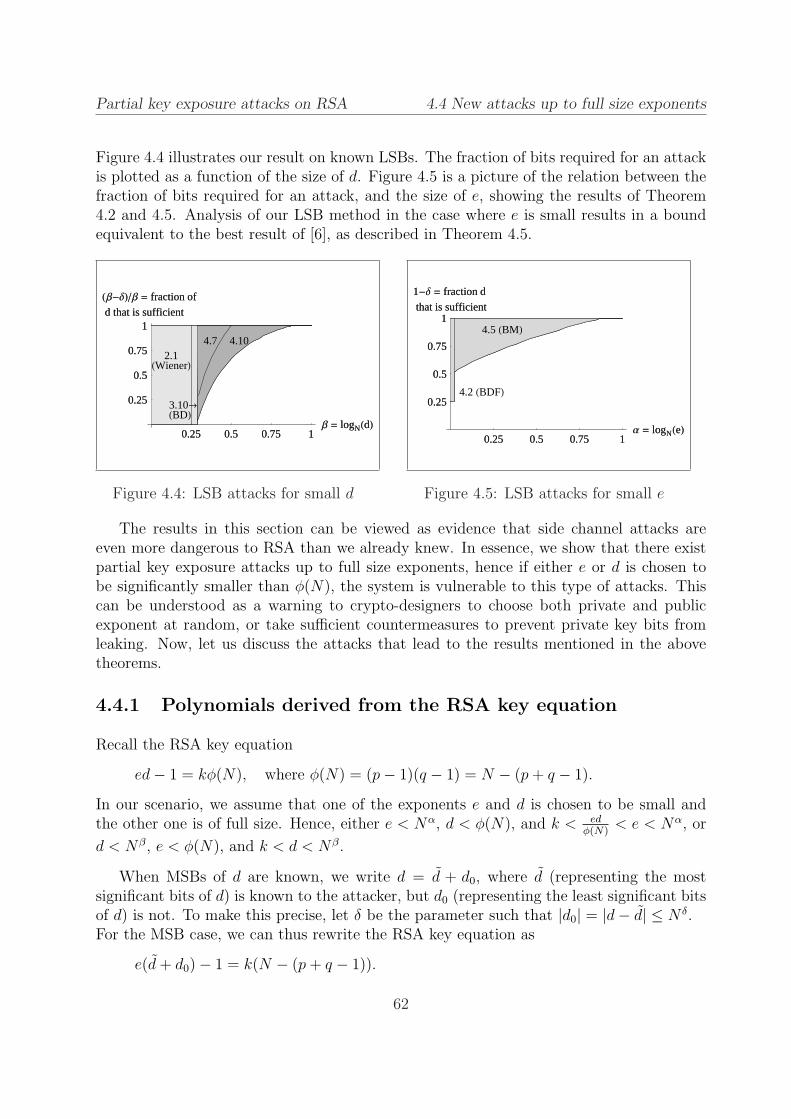
Partial key exposure attacks on RSA 4.4 New attacks up to full size exponents
Figure 4.4 illustrates our result on known LSBs. The fraction of bits required for an attackis plotted as a function of the size of d. Figure 4.5 is a picture of the relation between thefraction of bits required for an attack, and the size of e, showing the results of Theorem4.2 and 4.5. Analysis of our LSB method in the case where e is small results in a boundequivalent to the best result of [6], as described in Theorem 4.5.
0.25 0.5 0.75 1Β = logNHdL
0.25
0.5
0.75
1
HΒ-∆L�Β = fraction of
d that is sufficient
2.1HWienerL
3.10®HBDL
4.7 4.10
0.25 0.5 0.75 1Β = logNHdL
0.25
0.5
0.75
1
HΒ-∆L�Β = fraction of
d that is sufficient
Figure 4.4: LSB attacks for small d
0.25 0.5 0.75 1Α = logNHeL
0.25
0.5
0.75
1
1-∆ = fraction d
that is sufficient
4.2 HBDFL
4.5 HBML
0.25 0.5 0.75 1Α = logNHeL
0.25
0.5
0.75
1
1-∆ = fraction d
that is sufficient
Figure 4.5: LSB attacks for small e
The results in this section can be viewed as evidence that side channel attacks areeven more dangerous to RSA than we already knew. In essence, we show that there existpartial key exposure attacks up to full size exponents, hence if either e or d is chosen tobe significantly smaller than φ(N), the system is vulnerable to this type of attacks. Thiscan be understood as a warning to crypto-designers to choose both private and publicexponent at random, or take sufficient countermeasures to prevent private key bits fromleaking. Now, let us discuss the attacks that lead to the results mentioned in the abovetheorems.
4.4.1 Polynomials derived from the RSA key equation
Recall the RSA key equation
ed− 1 = kφ(N), where φ(N) = (p− 1)(q − 1) = N − (p + q − 1).
In our scenario, we assume that one of the exponents e and d is chosen to be small andthe other one is of full size. Hence, either e < Nα, d < φ(N), and k < ed
φ(N)< e < Nα, or
d < Nβ, e < φ(N), and k < d < Nβ.
When MSBs of d are known, we write d = d + d0, where d (representing the mostsignificant bits of d) is known to the attacker, but d0 (representing the least significant bitsof d) is not. To make this precise, let δ be the parameter such that |d0| = |d− d| ≤ N δ.For the MSB case, we can thus rewrite the RSA key equation as
e(d + d0)− 1 = k(N − (p + q − 1)).
62

Partial key exposure attacks on RSA 4.4 New attacks up to full size exponents
Hence, the polynomial
f(x, y, z) = ex−Ny + yz + (ed− 1)
has a root (x0, y0, z0) = (d0, k, p + q− 1). Then the root is ‘small’ since |x0| < X, |y0| < Y ,and |z0| < Z for some upper bounds X, Y, Z. In the case of RSA-Small-e, we have X = N δ,
Y = Nα, Z = N12 , neglecting the constants. For RSA-Small-d, the corresponding values
are X = N δ, Y = Nβ, and Z = N12 .
The attacker can also compute k = ed−1N
as an approximation to k and set k0 = k − kas the unknown part of k. It can be shown (analogous to the proof of Theorem 4.4) that
|k0| < eφ(N)
(d·3N− 12 +d0) <
{2Nα+δ−1 + 6Nα− 1
2 < 8Nγ, for γ = max{α + δ − 1, α− 12},
N δ + 3Nβ− 12 < 4Nγ, for γ = max{δ, β − 1
2}.
When we substitute the knowledge of the MSBs of k into the RSA key equation, we obtain
e(d + d0)− 1 = (k + k0)(N − (p + q − 1)).
Hence,
f(x, y, z) = ex−Ny + yz + kz + (ed− 1− kN)
has a root (x0, y0, z0) = (d0, k0, p + q − 1). With X = N δ, Y = Nγ, and Z = N12 , we
have |x0| < X, |y0| < Y , and |z0| < Z. Here, the value of γ is different in the cases ofRSA-Small-e and RSA-Small-d, as we showed above.
When LSBs of d are known, the attacker knows d ≡ d mod M for some M , and wewrite d = d + d1M , where d and M are known and d1 is not. We assume that d1 ≤ N δ.We have no approximation of k in this case, so we rewrite the RSA key equation as
e(d1M + d)− 1 = k(N − (p + q − 1)).
Thus,
f(x, y, z) = eMx−Ny + yz + (ed− 1)
has a root (x0, y0, z0) = (d1, k, p + q − 1). Then |x0| < X, |y0| < Y , and |z0| < Z, for some
X,Y, Z. For RSA-Small-e, we use X = N δ, Y = Nα, and Z = N12 , and for RSA-Small-d
these values are X = N δ, Y = Nβ, and Z = N12 . As before, we neglected the constants in
the definition of Y and Z, and let these constants contribute to some error term ε later.
4.4.2 Attacks for known MSBs and small d
1. Attack using no partial knowledge of k: proof of Theorem 4.8.1
We start by describing a method that finds a small root (x0, y0, z0) of f(x, y, z) = ex −Ny + yz + (ed − 1) over the integers, and prove the first result of Theorem 4.8, namelythat we have a polynomial time MSB attack when
δ <5
6− 1
3
√1 + 6β − ε.
63
Partial key exposure attacks on RSA 4.4 New attacks up to full size exponents
Since we have not yet given a detailed example of the general strategy for choosing theshifts for polynomials with integer roots, let us do so now. We will show that the boundfor which the roots of a polynomial f(x, y, z) = a0 + a1x + a2y + a3yz can be found inpolynomial time is
X1+3τY 2+3τZ1+3τ+3τ2
< W 1+3τ−ε,
for some τ ≥ 0 that can be optimized later.
We will use our (extended) strategy of Section 3.3.2, with extra z-shifts. First, we fixan integer m depending on ε and a parameter t, that we will optimize later in terms of m.
We define the set S as the monomials of fm−1 plus extra shifts of z. The set M issimply the set of all monomials that appear in xi1yi2zi3f(x, y, z) with xi1yi2zi3 ∈ S. Onecan check that
xi1yi2zi3 ∈ S ⇔ i1 = 0, . . . , m− 1 ; i2 = 0, . . . , m− 1− i1 ; i3 = 0, . . . , i2 + t,
xi1yi2zi3 ∈ M ⇔ i1 = 0, . . . , m ; i2 = 0, . . . , m− i1 ; i3 = 0, . . . , i2 + t,
defines such S and M as described above.
We denote by lj the largest exponent of xj that appears in the monomials of S,i.e. l1 = l2 = m − 1 and l3 = m − 1 + t. We have W = ‖f(xX, yY, zZ)‖∞ andR = (XY )m−1Zm−1+tW .
In order to work with a polynomial with constant term 1, we define
f ′(x, y, z) ≡ a−10 f(x, y, z) mod R = 1 + ax + by + cyz.
Next, we define the shift polynomials
g(x, y, z) := xi1yi2zi3f ′(x, y, z)Xm−i1Y m−i2Zm+t−i3 , for xi1yi2zi3 ∈ S,
g′(x, y, z) := xi1yi2zi3R , for xi1yi2zi3 ∈ M\S,
and let the coefficient vectors of g(x1X1, . . . xvXv) and g′(x1X1, . . . xvXv) form a latticebasis of a lattice L.
By the theory in Section 3.3.2, the following ordering of the monomials of S gives us atriangular matrix describing the lattice. We say that
xi11 · . . . · xiv
v < xi′11 · . . . · xi′v
v if∑
ij <∑
i′j.
If∑
ij =∑
i′j, then we use the lexicographical ordering. As a small example, we give thematrix corresponding to m = 2, t = 1. We have divided every row in the matrix by XY Z2
to get a cleaner view. The result is in Figure 4.6.
64

Partial key exposure attacks on RSA 4.4 New attacks up to full size exponents
1 x y z xz yz yz2 x2 xy xyz y2 y2z x2z xyz2 y2z2 y2z3
↓ ↓ ↓ ↓ ↓ ↓ ↓ ↓ ↓ ↓ ↓ ↓ ↓ ↓ ↓ ↓
1 aX bY cY Z1 aX bY cY Z
1 aX bY cY Z1 aX bY cY Z
1 bY aX cY Z1 aX bY cY Z
1 aX bY cY Z
WX2
WXYWXY Z
WY 2
WY 2ZWX2Z
WXY Z2
WY 2Z2
WY 2Z3
Figure 4.6: Example: Matrix for m = 2, t = 1
From Section 3.3.2, we know that
Xs1Y s2Zs3 < W sW−ε, for sj =∑
xi1yi2zi3∈M\Sij , and sW = |S|.
suffices for the polynomials r1, r2 corresponding to the smallest vectors in the reducedlattice basis of L to satisfy ri(x
(0)1 , . . . , x
(0)v ) = 0. Under Assumption 3.7, the resultant
computations of f , r1, and r2 will reveal the root.
With the given definitions for S and M , we find the asymptotic bound
X16m3(1+3τ)+o(m3)Y
16m3(2+3τ)+o(m3)Z
16m3(1+3τ+3τ2)+o(m3) < W
16m3(1+3τ)+o(m3),
which reduces to
X1+3τY 2+3τZ1+3τ+3τ2
< W 1+3τ−ε,
for m →∞, if we let all terms of order o(m3) contribute to ε.
Finally, we come to the result of our partial key exposure attack on RSA-Small-d usingf(x, y, z) = ex − Ny + yz + (ed − 1). In our case, X = N δ, Y = Nβ, Z = N
12 and
W = max{eX, NY, Y Z, R} ≥ NY = N1+β. Hence, the asymptotic bound to satisfy is
δ(1 + 3τ) + β(2 + 3τ) +1
2(1 + 3τ + 3τ 2) < (1 + β)(1 + 3τ),
65

Partial key exposure attacks on RSA 4.4 New attacks up to full size exponents
or equivalently
3τ 2 + 3τ(2δ − 1) + (2δ + 4β − 1) < 0.
We find an optimal value τ = 12− δ, which implies δ < 5
6− 1
3
√1 + 6β. Thereby, we have
derived the result of Theorem 4.8.1.
2. Attack using partial knowledge of k: proof of Theorem 4.8.2 and 4.8.3
We will now show how to obtain the second and third result mentioned in Theorem 4.8,namely that we have a polynomial time MSB attack whenever
δ <3
16− ε and β ≤ 11
16, or δ <
1
3+
1
3β − 1
3
√4β2 + 2β − 2− ε and β ≥ 11
16.
For the situation where we use information on MSBs of d to get an approximation k of k,we want to find a small root (x0, y0, z0) of the polynomial
f(x, y, z) = ex−Ny + yz + kz + (ed− 1− kN).
We will use the extended strategy as described in Section 3.3.2 with extra shifts of y. For apolynomial f(x, y, z) = a0 +a1x+a2y+a3z+a4yz, the sets S and M can then be describedby
xi1yi2zi3 ∈ S ⇔ i1 = 0, . . . , m− 1 ; i2 = 0, . . . , m− 1− i1 + t ;i3 = 0, . . . , m− 1− i1
xi1yi2zi3 ∈ M ⇔ i1 = 0, . . . , m ; i2 = 0, . . . , m− i1 + t ; i3 = 0, . . . , m− i1
for fixed m (depending on ε) and some t = τm that will be optimized later.Substituting this in bound (3.7), we obtain
X2+3τY 3+6τ+3τ2
Z3+3τ < W 2+3τ−ε.
In our case, we have X = N δ, Y = Nγ, with γ = max{δ, β − 12}, and Z = N
12 . Also,
W = max{eX, NY, Y Z, kZ, R} ≥ NY = N1+γ. The optimal value τ =12−δ−γ
2γleads to the
condition
δ <1
3γ +
1
2− 1
3
√4γ2 + 6γ.
If γ = δ, this implies
δ <3
16.
Note that this bound is only valid if max{δ, β − 12} = δ, which implies that β ≤ 11
16.
If γ = β − 12, we get
δ <1
3+
1
3β − 1
3
√4β2 + 2β − 2 , valid for β ≥ 11
16.
This concludes the proof of Theorem 4.8.
66

Partial key exposure attacks on RSA 4.4 New attacks up to full size exponents
4.4.3 Attacks for known MSBs and small e
Many users of RSA choose a small public exponent e. Therefore, we now let e = Nα
and d < φ(N) and investigate the possibilities for new partial key exposure attacks forRSA-Small-e. The best result in this situation, as mentioned in Theorem 4.9, is that weobtain a polynomial time MSB attack whenever
δ <1
3+
1
3α− 1
3
√4α2 + 2α− 2− ε for α >
1
2.
We can again use the polynomial of the attack without partial knowledge of k, thatis, f(x, y, z) = ex − Ny + yz + (ed − 1), now with X = N δ, Y = Nα and Z = N
12 . We
will substitute all this, and W = N1+α in the bound that we obtained for this polynomial,namely
X1+3τY 2+3τZ1+3τ+3τ2
< W 1+3τ−ε.
As this case is completely similar to the case of small d, we find the bound
δ <5
6− 1
3
√1 + 6α− ε.
This result only holds for α > 12. In the case that α < 1
2, we know from Theorem 4.4 that
we can assume that k is known. Hence, the polynomial to be analyzed becomes bivariate.Since our attack using no partial knowledge of k obtains a bound inferior to the one
using the approximation of k that can be derived, it is not mentioned in Theorem 4.9. Thisbrings us to the description of the attack using partial information on k.
Attack using partial knowledge of k: proof of Theorem 4.9
When we use partial information on k, where k is partly unknown (so α > 12), we can use
f(x, y, z) = ex−Ny + yz + kz + (ed− 1− kN).
We have X = N δ, Y = Nγ, with γ = max{α + δ − 1, α − 12}, and Z = N
12 . Using
W = N1+γ, we get the same condition as in the previous paragraph, namely
δ <1
3γ +
1
2− 1
3
√4γ2 + 6γ − ε.
We analyze this for two possibilities of γ.If we substitute γ = α + δ − 1 (in other words, we assume δ > 1
2), we obtain the
condition
δ <3 + 4α− 4α2
16α− ε.
However, for α > 12, δ < 3+4α−4α2
16α< 1
2, so we get no result.
If γ = α− 12, we find
δ <1
3+
1
3α− 1
3
√4α2 + 2α− 2− ε.
This concludes the proof of Theorem 4.9.
67

Partial key exposure attacks on RSA 4.4 New attacks up to full size exponents
4.4.4 Attack for known LSBs and small d
In this section, we will show how to obtain the result of Theorem 4.10, namely that wehave a polynomial time LSB attack whenever
δ <5
6− 1
3
√1 + 6β − ε.
Attack description: proof of Theorem 4.10
Polynomial f(x, y, z) = eMx−Ny +yz +(ed−1) has the same monomials as in the MSB-attack where no partial knowledge of k was used. So, we can directly apply the knownanalysis for a polynomial with monomials 1, x, y, yz. We use
X1+3τY 2+3τZ1+3τ+3τ2 ≤ W 1+3τ−ε,
on X = N δ, Y = Nβ, Z = 3N12 and W = max{eMX, NY, Y Z,R} ≥ NY = N1+β. This
implies
δ <5
6− 1
3
√1 + 6β.
This concludes the proof of Theorem 4.10.
If we adapt the LSB attack for the situation when e is not of full size, we get exactlythe result from Blomer and May in Theorem 4.5.
4.4.5 Experiments for the new attacks
We state some experimental results to give an idea of the performance of our methods.In the following three examples, N ≈ 21024. The experiments are performed on a servercontaining two Pentium III processors of 1000 Mhz, and all the lattice basis reductions aredone using Shoup’s NTL [66].
For our attack on small d without using partial knowledge of k, a typical case is β = 0.3and δ = 0.21 (e.g. 70% of d is unknown). An attack using m = 3, t = 1 involved a 10minute reduction of the 30-dimensional lattice.
We performed an attack on small d using partial knowledge of k for β = 0.6, δ = 0.13(e.g. 22% of d is unknown), with m = 3, t = 2. The 50-dimensional lattice took 31
4hours
to reduce.We performed the attack on small e using partial knowledge of k for α = 0.7, δ = 0.08
(e.g. 8% of d is unknown), using m = 3, t = 2. The reduction of the 50-dimensional latticetook 23
4hours.
More experimental results are included in the following tables, but now for a moduluslength of 256 bits. As the bounds on δ stated in the theorems are asymptotic bounds, thegoal of the tables is to provide some insight of what values of δ our attacks can realize inpractice. Note that the LLL reduction time for a larger modulus length is longer, so theattacks will take longer when performed on N ≈ 21024 or N ≈ 22048.
68

Partial key exposure attacks on RSA 4.4 New attacks up to full size exponents
β δ m = 2 m = 3asympt. t = 0 t = 1 t = 2 t = 0 t = 1 t = 2
0.30 0.28 0.19 0.19 0.19 0.19 0.21 0.210.35 0.25 0.13 0.14 0.14 0.14 0.16 0.160.40 0.22 0.09 0.11 0.11 0.09 0.14 0.150.45 0.19 0.04 0.10 0.10 0.05 0.12 0.120.50 0.17 0 0.08 0.09 0 0.10 0.110.55 0.14 0 0.08 0.08 0 0.09 0.110.60 0.12 0 0.04 0.04 0 0.06 0.100.65 0.10 0 0 0 0 0 0.060.70 0.07 0 0 0 0 0 0.010.75 0.05 0 0 0 0 0 00.80 0.03 0 0 0 0 0 00.85 0.01 0 0 0 0 0 0
Dimension: 10 16 22 20 30 40LLL (sec): 1 2 8 3 25 100
Table 4.2: Experiments for small d, not using partial knowledge of k
β δ m = 2 m = 3asympt. t = 0 t = 1 t = 2 t = 3 t = 0 t = 1 t = 2
0.30 0.19 0.19 0.20 0.20 0.20 0.19 0.19 0.190.35 0.19 0.15 0.16 0.16 0.16 0.16 0.16 0.160.40 0.19 0.12 0.12 0.12 0.12 0.14 0.15 0.150.45 0.19 0.10 0.11 0.12 0.12 0.12 0.13 0.130.50 0.19 0.08 0.11 0.12 0.12 0.12 0.13 0.130.55 0.19 0.08 0.11 0.12 0.12 0.11 0.13 0.130.60 0.19 0.05 0.11 0.11 0.11 0.11 0.12 0.130.65 0.19 0 0.05 0.06 0.06 0.05 0.08 0.100.70 0.18 0 0 0 0 0 0.04 0.050.75 0.14 0 0 0 0 0 0 00.80 0.11 0 0 0 0 0 0 00.85 0.08 0 0 0 0 0 0 00.90 0.05 0 0 0 0 0 0 00.95 0.03 0 0 0 0 0 0 0
Dimension: 14 20 26 32 30 40 50LLL (sec): 1 7 17 40 26 180 480
Table 4.3: Experiments for small d, using partial knowledge of k
When we are in the area of the key space where the 2-dimensional attack applies, thismethod is clearly faster, and should be preferred over the attacks using larger lattices.
69

Partial key exposure attacks on RSA 4.4 New attacks up to full size exponents
α δ m = 2 m = 3asymptotic t = 0 t = 1 t = 2 t = 3 t = 0 t = 1 t = 2
0.50 0.50 0.25 0.33 0.38 0.40 0.32 0.37 0.410.55 0.33 0.17 0.21 0.23 0.25 0.21 0.23 0.240.60 0.27 0.09 0.14 0.17 0.18 0.13 0.16 0.190.65 0.22 0.02 0.07 0.10 0.10 0.07 0.11 0.130.70 0.18 0 0.02 0.03 0.04 0.02 0.04 0.080.75 0.14 0 0 0 0 0 0.01 0.020.80 0.11 0 0 0 0 0 0 00.85 0.08 0 0 0 0 0 0 00.90 0.05 0 0 0 0 0 0 00.95 0.03 0 0 0 0 0 0 0
Dimension: 14 20 26 32 30 40 50LLL (sec): 1 5 13 40 33 180 520
Table 4.4: Experiments for small e, using partial knowledge of k
Concerning the choice of t, recall that t = τm, and that we use τ = 12− δ to obtain the
asymptotic result of our RSA-Small-d attack using no partial knowledge of k. This explainsthat for m = 2 in Table 4.2, a value of t larger than 1 gives no significant improvement,but for m = 3, t = 2 may give a better result when the bound on δ is ‘low’. For the
attacks using partial knowledge of k, the optimal value of τ is τ =12−δ−γ
2γ. This explains
for example, that when e = Nα with α close to 12, a larger value of t gives a better bound
on δ in the experiments (as can be seen in Table 4.4).
After these experiments, we are now ready to comment on Assumption 3.7. Letr1(x, y, z) and r2(x, y, z) be polynomials that correspond to the smallest LLL reducedvectors in our method. If we assume that Howgrave-Graham’s bound is satisfied for both,then r1(x0, y0, z0) = r2(x0, y0, z0) = 0. Now Assumption 3.7 does not hold when the re-sultant computations with r1 and r2 yield the zero polynomial. Therefore, we performedsome tests to see how often this occurs. We found that for small δ, approximately 0.1%of pairs (r1, r2) the heuristic failed. However, Bauer and Joux [2] recently showed that forlarger δ, the heuristic fails more often. For example, let us look at the attack on small dwithout using knowledge of k (Table 4.2). In the attack for m = 2, t = 1, β = 0.35 andδ = 0.10, the heuristic fails in about 20% of the cases. This does not mean that the wholeattack will fail in these cases. The method finds about 10 polynomials ri that are smallenough to have the root over the integers, and if r1 and r2 are algebraically dependent, wejust try other combinations until the resultant method succeeds. In Section 5.3, we show arelaxation of Assumption 3.7 with the same idea. For the attack to succeed, we only needtwo independent ri’s that satisfy ri(x0, y0, z0) = 0, they do not have to be r1 and r2. For aprovable way to find a third independent polynomial r2 from f and r1 in the case of thisattack, we refer to the paper of Bauer and Joux [2].
70

Partial key exposure attacks on RSA 4.5 Tabular overview
Experiments also show that the theoretical bound under which our methods works,
det(L) ≤ (2−ω4
1√ω
)ω−1Rω−1,
is far too strict. It would imply that for m ∈ {2, 3}, the method will never work, which
clearly contradicts the practice. This is both due to the term (2−ω4
1√ω)ω−1, when it is known
that LLL reduction achieves much better bounds in practice, and to the fact that we usethe LLL bound for the second smallest reduced vector. In practice, we experienced thatour method works until det(L) comes close to Rω (the upper bound for the first reducedvector to be small enough, omitting the terms that do not depend on N).
Apparently, the lattice L satisfies Assumption 3.3 in this case. Because the lattice isbalanced, all reduced vectors (especially the smallest vectors) have a norm of approximately
det(L)1ω and the bound det(L)
1ω < R describes the cases for which the attack works in
practice.
4.5 Tabular overview
The following tables include all known and new partial key exposure attacks on RSA-Small-e and RSA-Small-d respectively.
Type of attack Attack bound Reference
known MSBs δ < 1− α and α ∈ (14, 1
2) Thm. 4.3.1/4.3.2
δ < α and α ≤ 12
Thm. 4.3.3
δ < 14
and α ≤ 12
Thm. 4.3.4
δ < 18(5− 2α−√36α2 + 12α− 15)− ε and Thm. 4.6
α ∈ (12,√
6−12
)
δ < 13
+ 13α− 1
3
√4α2 + 2α− 2− ε and Thm. 4.9
α ∈ (12, 1)
known LSBs δ < 34
and e = poly(n) Thm. 4.2
δ < 56− 1
3
√1 + 6α− ε and α ∈ (0, 7
8) Thm. 4.5
Table 4.5: Partial key exposure attacks for RSA-Small-e
71

Partial key exposure attacks on RSA 4.5 Tabular overview
Type of attack Attack bound Reference
no bits necessary β < 0.25 WienerThm. 2.1
β < 0.292− ε Boneh/DurfeeThm. 3.10
known MSBs/LSBs δ < 12− β Thm. 4.7
known MSBs δ < 56− 1
3
√1 + 6β − ε Thm. 4.8.1
δ < 316− ε and β ≤ 11
16Thm. 4.8.2
δ < 13
+ 13β − 1
3
√4β2 + 2β − 2− ε and β > 11
16Thm. 4.8.3
known LSBs δ < 56− 1
3
√1 + 6β − ε Thm. 4.10
Table 4.6: Partial key exposure attacks for RSA-Small-d
72

5Attacks on RSA-CRT variants
In this chapter we discuss the known attacks on RSA-CRT variants. Moreover, we discuss anew attack on CRT-Small-dp, dq (that also affects the security of CRT-BalancedExponents),and a new attack on CRT-Qiao&Lam.
Section 5.3 is based on [37] and Section 5.4 is based on [38], both of which are jointpapers with Alexander May.
5.1 Introduction
As we have mentioned before, in many implementation proposals of the RSA cryptosystem,either the public exponent e or the private exponent d is chosen to be small. Since theattacks of Wiener [75] and Boneh and Durfee [10] on RSA-Small-d, we know that choosing asmall d can be dangerous. As an alternative approach, Wiener proposed to use the ChineseRemainder Theorem (CRT) for decryption/signing, and ‘small private CRT-exponents’instead of a small private exponent. The new decryption/signing process of RSA, asproposed by Quisquater and Couvreur in [61] then works in the following way:
• ‘split’ the private exponent d into dp ≡ d mod (p− 1) and dq ≡ d mod (q − 1),
• decrypt/sign by first computing
mp ≡ cdp mod p and mq ≡ cdq mod q,
and then using CRT to compute the unique value m modulo N such that
m ≡ mp mod p and m ≡ mq mod q.
RSA using CRT is specifically useful in time-critical applications, for instance for sign-ing procedures on smartcards. As for the security of RSA variants using CRT, thereexists a meet-in-the-middle attack enabling the adversary to factor N in time and spaceO(min{√dp,
√dq}), which is exponential in the bitsize of the minimum of dp and dq,
see [8, 51]. We use the “soft-O” notation here, which ignores the logarithmic factors.
Let us briefly recall some RSA-CRT variants, for which we shall discuss the knownattacks in Section 5.2, and new attacks on some of these variants in Section 5.3 and 5.4.
73

Attacks on RSA-CRT variants 5.1 Introduction
Standard RSA-CRT (“CRT-Standard”):
In all RSA-CRT variants, the RSA-CRT parameters e, dp, dq, p, q satisfy
edp ≡ 1 mod (p− 1) and edq ≡ 1 mod (q − 1).
If all parameters are chosen generically, then we have
edp = 1 + kp(p− 1) and edq = 1 + kq(q − 1),
for e ≈ N, p ≈ q ≈ dp ≈ dq ≈ N12 , kp ≈ kq ≈ N .
RSA-CRT with small public exponent e (“CRT-Small-e”) :
As in standard RSA, it is possible to choose a small e, after which the Extended EuclideanAlgorithm finds the corresponding d, which in turn is then split up in dp and dq. If onechooses p and q first at random, and then a small e, then the private CRT-exponents dp
and dq will be about as long as p and q in general. So, we have
e ≈ Nα, p ≈ q ≈ dp ≈ dq ≈ N12 , kp ≈ kq ≈ Nα, for α < 1.
RSA-CRT with small private CRT-exponents dp, dq (“CRT-Small-dp, dq”) :
This variant was proposed by Wiener in [75] as a possible alternative to using a smalldecryption exponent d. In this case, one assumes that the decryption/signing time iscritical. First one picks p and q as random primes of bitsize 1
2n, and dp and dq as random
integers of a certain small bitsize such that they are coprime to p− 1 and q− 1. Then onecan compute d smaller than φ(N) such that d ≡ dp mod (p − 1) and d ≡ dq mod (q − 1).From this d, one can compute the corresponding e as usual.
Hence, the setting is: e is full size, p and q are balanced, and dp and dq are balancedbut significantly smaller than p and q. So, we have
e ≈ N, p ≈ q ≈ N12 , dp ≈ dq ≈ Nβ, kp ≈ kq ≈ Nβ+ 1
2 , for β <1
2.
It has been an open question since Wiener’s work whether or not there exist polynomialtime attacks on RSA-CRT with small CRT-exponents. In Section 5.3, we give an affirma-tive answer to this question, when we describe a new attack that works for β < 0.0734.
RSA-CRT with unbalanced primes (“CRT-UnbalancedPrimes”) :
This variant was studied by May [52], who found the first polynomial time attacks on anRSA-CRT case. In this scenario, the idea is to minimize the cost of the decryption mod qby taking a small q, and to minimize the cost of the decryption mod p by taking a small dp.Hence, the setting is: e is full size, p and q are unbalanced (where q is the smaller prime),and dp is significantly smaller than p. So,
e ≈ N, p ≈ N1−γ, q ≈ Nγ, dp ≈ Nβ, dq < Nγ, kp ≈ Nβ+γ, kq ≈ N,
for γ < 12
and β < 1− γ.
74

Attacks on RSA-CRT variants 5.1 Introduction
RSA-CRT with small e and small dp and dq (“CRT-BalancedExponents”) :
This variant, proposed by Galbraith/Heneghan/McKee [28] and Sun/Wu [70], balances thecost of decryption and encryption, by enabling an implementor of the key generation tochoose e and dp and dq smaller than standard. In Section 2.2, we discussed a possible keygeneration method for this variant.
The general setting is: e is relatively small, p and q are balanced, and dp and dq arebalanced but smaller than p and q. So,
e ≈ Nα, p ≈ q ≈ N12 , dp ≈ dq ≈ Nβ, kp ≈ kq ≈ Nα+β− 1
2 , for α < 1 and β <1
2.
In the papers [28] and [70], the authors describe various attacks, and propose parametersfor which the mentioned attacks do not work. A new attack by Bleichenbacher and May [4]made the authors of the proposals change their parameter choices [27, 69]. Our new attack,described in Section 5.3, leads to another part of the key space that should be consideredunsafe.
RSA-CRT with small difference dp − dq (“CRT-Qiao&Lam”) :
Qiao and Lam [60] proposed to use CRT-Small-dp, dq and to use dq = dp − 2. In this way,one profits from the fast decryption method of CRT-Small-dp, dq, while one only has tostore one of the two private CRT-exponents. In Section 5.4 we describe a new attack onthis variant.
If we now summarize the five possible ways to speed up either encryption/verifying ordecryption/signing (or both), the general setting is as follows.
{edp = 1 + kp(p− 1),edq = 1 + kq(q − 1),
with
e ≈ Nα for 0 < α ≤ 1p ≈ N1−γ for 0 < γ ≤ 1
2
q ≈ Nγ
dp ≈ Nβ for 0 < β ≤ 1− γ
dq ≈ Nκ for κ =
{β, if γ = 1
2
γ, if γ < 12
kp ≈ Nα+β+γ−1
kq ≈ Nα+κ−γ
The default values for the parameters are α = 1, γ = β = κ = 12, and for special
RSA-CRT settings described above, the parameters are as below.
75
Attacks on RSA-CRT variants 5.2 Known attacks
CRT-Small-e: α < 1, γ = β = κ = 12.
CRT-Small-dp, dq: α = 1, γ = 12, β = κ < 1
2.
CRT-UnbalancedPrimes: α = 1, γ = κ < 12, β < 1− γ.
CRT-BalancedExponents: α < 1, γ = 12, β = κ < 1
2.
CRT-Qiao&Lam: see CRT-Small-dp, dq.
In the next section we will look at the known attacks on the RSA-CRT variants. We willgive short descriptions of each attack in the most general setting possible, and explore forwhich values of the parameters (and therefore for which variants) the attacks work.
5.2 Known attacks
In this section, we briefly discuss the attacks proposed in the literature on the subject. Wegive the theorems in the general setting in order to see if an attack that is designed for oneCRT variant may be applicable to another CRT variant.
It is important to note that α + β + γ − 1 ≥ 0 and α + κ− γ ≥ 0, since kp and kq arepositive integers. In the CRT-BalancedPrimes variant, it may happen that α + β − 1
2≈ 0,
which means that kp and kq are very small, and must be assumed to be public knowledge.Since it makes no sense to treat kp and kq as variables in an equation if they are known, wemake a distinction between attacks with unknown kp, kq, and attacks with known kp, kq.
First, we start with the attacks on RSA-CRT variants where kp and kq are not known.To introduce the notation for all of these attacks, we use the following condition.
Condition (*) (Notation for the known attacks on RSA-CRT variants)Let N = pq be an n-bit RSA modulus. Let 0 < α ≤ 1, 0 < γ ≤ 1
2, 0 < β ≤ 1
2, and
0 < κ ≤ 12
such that κ = γ if γ < 12
and κ = β if γ = 12. Let p, q be primes of bitsize
(1 − γ)n and γn. Furthermore, let e, dp, dq satisfy edp ≡ 1 mod (p − 1) and edq ≡ 1mod (q − 1) with bitsize(e) = αn, bitsize(dp) = βn, and bitsize(dq) = κn.
The following attack was originally meant for the CRT-UnbalancedPrimes setting.
Theorem 5.1 (May, [52])Under Assumption 3.7, for every ε > 0, there exists an integer n0 such that for everyn > n0, the following holds: Consider an RSA-CRT instance satisfying (*). Then N canbe factored in time polynomial in n when:
β <1
2(2− 3γ + γ2 − α)− ε.
76

Attacks on RSA-CRT variants 5.2 Known attacks
Proof.For the attack, May notices that edp + (kp − 1) ≡ 0 mod p, hence
fp(x, y) = ex− y has a small root (dp, kp − 1) modulo p.
In this thesis, we have not discussed Coppersmith methods for small roots modulo anunknown modulus p, of which one knows a multiple N . However, these methods exist(see [13, 54]), and May shows that using the shifts
gjk(x, y) = xjNmax{0,τm−k}fkp (x, y), for k = 0, . . . ,m− 1, j = m− k − 1,
one finds the bound
(XY )12 < pτN− 1
2τ2−ε.
For p = N1−γ, X = Nβ, Y = Nα+β+γ−1 the optimal value of τ is τ = 1− γ. It follows that
β <1
2(2− 3γ + γ2 − α)− ε.
2
For CRT-UnbalancedPrimes, the bound of Theorem 5.1 reduces to May’s result [52]
β <1
2(1− 3γ + γ2)− ε.
For CRT-BalancedExponents, it follows that
β <3
8− 1
2α− ε
is unsafe. CRT-Small-e and CRT-Small-dp, dq are not affected.
The second attack by May, a result described in the following theorem, was also origi-nally meant for the setting of CRT-UnbalancedPrimes.
Theorem 5.2 (May, [52])Under Assumption 3.7, for every ε > 0, there exists an integer n0 such that for everyn > n0, the following holds: Consider an RSA-CRT instance satisfying (*). Then N canbe factored in time polynomial in n when:
β < 1− 2
3γ − 2
3
√γ2 + 3γα− ε.
Proof.To obtain this result, May looks at the equation edp = 1 + kp(p− 1) modulo e. Hence,
kp(p− 1) + 1 ≡ 0 mod e.
77

Attacks on RSA-CRT variants 5.2 Known attacks
If this is multiplied by q, then the result is
kp(N − q) + q ≡ 0 mod e, or equivalently
(kp − 1)N − (kp − 1)q + N ≡ 0 mod e.
Thus, fe(x, y) = x(N − y) + N has a small root (x0, y0) = (kp − 1, q) modulo e. This is apolynomial a la Boneh/Durfee (see Section 3.3.1), and the known bound is
X2+3τY 1+3τ+3τ2
< e1+3τ−ε.
For X = Nα+β+γ−1, Y = Nγ, the optimal τ = 1−2γ−β2γ
leads to the bound
β < 1− 2
3γ − 2
3
√γ2 + 3γα− ε.
2
For CRT-UnbalancedPrimes, the bound of Theorem 5.2 reduces to
β < 1− 2
3γ − 2
3
√γ2 + 3γ − ε.
For the setting of CRT-BalancedExponents, it leads to the bound
β <2
3− 1
3
√1 + 6α− ε.
This last bound implies that α+β < 12, so therefore it has no consequences for the security
of CRT-BalancedExponents.
The last attack that was proposed for the CRT-UnbalancedPrimes case is by Bleichen-bacher and May.
Theorem 5.3 (Bleichenbacher/May, [4])Under Assumption 3.7, for every ε > 0, there exists an integer n0 such that for everyn > n0, the following holds: Consider an RSA-CRT instance satisfying (*). Then N canbe factored in time polynomial in n when:
β <1
3(3− 2γ − γ2 −
√12αγ − 12αγ2 + 4γ2 − 5γ3 + γ4)− ε.
Proof sketch.Bleichenbacher and May improved the attack of Theorem 5.2 in their paper [4]. Theyobserve that the shifts that are used for polynomial fe(x, y) = x(N − y) + N , namely
gijk(x, y) = xiyjfk(x, y)em−k,
contains many powers of y. The y0 that one is looking for, namely y0 = q, satisfies y0·p = N .Therefore, Bleichenbacher and May introduce a new variable z for p, and use the shifts
gijk(x, y, z) = xiyjzsfk(x, y)em−k,
78

Attacks on RSA-CRT variants 5.2 Known attacks
for a value of s that has to be optimized. Moreover, since y0 · z0 = N , they replace everyoccurrence of yz by N . For a detailed analysis of the determinant of the lattice that follows,and a proof of this theorem, we refer to [4].
2
For CRT-UnbalancedPrimes, the above result reduces to
β <1
3(3− 2γ − γ2 −
√12γ − 8γ2 − 5γ3 + γ4)− ε.
For CRT-BalancedExponents, it leads to an attack bound
β <7
12− 1
12
√7 + 48α− ε.
Let us now move on to the known attacks that were designed for CRT-BalancedExponents.The following attack features in both proposals of the CRT-BalancedExponents case.
Theorem 5.4 (GHM and SW, [28, 70])Under Assumption 3.7, for every ε > 0, there exists an integer n0 such that for everyn > n0, the following holds: Consider an RSA-CRT instance satisfying (*). Then N canbe factored in time polynomial in n when:
β < 1 + γ − 2κ− 2α− ε.
Proof.For this attack, the equations
kpp ≡ kp − 1 mod e and kqq ≡ kq − 1 mod e
are multiplied with each other. This results in
kpkq(N − 1) + kp + kq − 1 ≡ 0 mod e,
which means that the polynomial fe(u, v) = u(N−1)+v has a small root (kpkq, kp +kq−1)modulo e. This is a simple case of a polynomial where the total degree is 1 (a specific case ofthe “generalized lower triangle”, treated in Section 3.3.1). The bound that can be derivedfrom the discussion of generalized lower triangles in Section 3.3.1 is
UV < e1−ε.
Substituting U = N2α+β+κ−1 and V = Nα+κ−γ, one obtains
β < 1 + γ − 2κ− 2α− ε.
2
79

Attacks on RSA-CRT variants 5.2 Known attacks
For {γ = 12, κ = β}, it follows that the above attack works for
β <1
2− 2
3α− ε
which is only applicable in the CRT-BalancedExponents setting. For {γ < 12, κ = γ}, it
gives
β < 1− 2α− γ − ε,
which doesn’t affect CRT-UnbalancedPrimes.
The attack by Bleichenbacher and May originally meant for CRT-BalancedExponents isdescribed in the following theorem.
Theorem 5.5 (Bleichenbacher/May, [4])Under Assumption 3.7, for every ε > 0, there exists an integer n0 such that for everyn > n0, the following holds: Consider an RSA-CRT instance satisfying (*). Then N canbe factored in time polynomial in n when:
β <1
2(1 + 2γ − 2α− 3κ)− ε.
Proof.In the latest result on CRT-BalancedExponents, Bleichenbacher and May follow the stra-tegy of Theorem 5.4, except that they do not look at the equations modulo e. That is,they multiply the equations
edp + kp − 1 = kpp and edq + kq − 1 = kqq
with each other, which results in the equation
e2dpdq + edp(kq − 1) + edq(kp − 1)− (N − 1)kpkq − (kp + kq − 1) = 0.
Then, (x(0)1 , x
(0)2 , x
(0)3 , x
(0)4 ) = (dpdq, dp(kq − 1) + dq(kp − 1), kpkq, kp + kq − 1) is a root of
f(x1, x2, x3, x4) = e2x1 + ex2 − (N − 1)x3 − x4 = 0.
This is simply a linear polynomial, whose known bound is
X1X2X3X4 < W 1−ε,
for W = N2α+β+κ, X1 = Nβ+κ, X2 = Nα+β+κ−γ, X3 = N2α+β+κ−1, X4 = Nα+κ−γ. Thisimmediately leads to the bound given in this theorem.
2
For {γ = 12, κ = β}, it follows that the attack works for
β <2
5− 2
5α− ε
80

Attacks on RSA-CRT variants 5.2 Known attacks
which is only applicable in the CRT-BalancedExponents setting. For {γ < 12, κ = γ}, it
gives
2α + 2β + γ < 1,
which doesn’t affect the CRT-UnbalancedPrimes case.
Having discussed many attacks for the RSA-CRT cases with unknown kp, kq, we nowsummarize the best known result for the case that kp and kq are known.
Theorem 5.6 (GHM, [28])Let N = pq be an n-bit RSA modulus, where p and q are primes of equal bitsize. Let0 < α < 1 and 0 < β ≤ 1
2. Furthermore, let e, dp, dq satisfy edp = 1 + kp(p − 1)
and edq = 1 + kq mod (q − 1) with bitsize(e) = αn, and bitsize(dp) = bitsize(dq) = βn.Suppose that kp and kq are very small, that is α + β − 1
2≈ 0. Then N can be factored in
time polynomial in n when:
α >1
4.
Proof.The attack originates from Coppersmith’s attack that uses partial knowledge of p. Namely,when kp and kq are known, then one knows
p ≡ k−1p (kp − 1) mod e and q ≡ k−1
q (kq − 1) mod e.
When e > N14 , then Theorem 4.1 says that one can find p.
2
0.25 0.5Γ = logNHqL
0.25
0.5
0.75
1
Β = logNHdpL
5.15.3
5.2
0.25 0.5Γ = logNHqL
0.25
0.5
0.75
1
Β = logNHdpL
Figure 5.1: CRT-UnbalancedPrimes
0.25 0.5 0.75 1Α = logNHeL
0.25
0.5
Β = logNHdpL
5.5
5.4
5.3 ®
5.1 ®
0.25 0.5 0.75 1Α = logNHeL
0.25
0.5
Β = logNHdpL
Figure 5.2: CRT-BalancedExponents
81

Attacks on RSA-CRT variants 5.3 A new attack on CRT-Small-dp, dq
This concludes the discussion of all known polynomial time attacks on CRT variants. Notethat up to now, there only exist polynomial time attacks on CRT-UnbalancedPrimes andCRT-BalancedExponents. Figure 5.1 and 5.2 give an overview of the attacks on thesevariants. The numbers in the figures refer to the respective theorems.
Besides the ‘normal’ polynomial time attacks on RSA-CRT variants, there also existpartial key exposure attacks. The known partial key exposure attacks from Blomer andMay [6] on CRT-Small-e are summarized in the next theorem. For a proof of this theorem,we refer to [6].
Theorem 5.7 (Blomer/May, [6])For every ε > 0, there exists an integer n0 such that for every n > n0, the following holds:Let N = pq be an n-bit RSA modulus, where p and q are primes of equal bitsize. Let0 < α < 1, 0 < β ≤ 1
2, and 0 < δ < β. Furthermore, let e, dp, dq satisfy edp = 1+kp(p−1)
and edq = 1 + kq mod (q − 1) with bitsize(e) = αn.
1. Suppose an attacker knows MSBs of dp, and suppose the unknown LSB-part of dp isof size N δ. Then N can be factored in time polynomial in n when:
δ <1
4− α− ε.
2. Suppose an attacker knows LSBs of dp, and suppose the unknown MSB-part of dp isof size N δ. Moreover, suppose that e is of size poly(n) such that all possible kp can betried out in polynomial time. Then N can be factored in time polynomial in n when:
δ <1
4− ε.
5.3 A new attack on CRT-Small-dp, dq
In this section, we discuss a new attack on CRT-Small-dp, dq. Recall that all attacks in theprevious section were not applicable in the standard RSA case with small CRT-exponentsdp and dq, that is, when p and q are balanced and e is full size. Here, we describe a wayto extend one of the attacks of Bleichenbacher/May [4] such that it also works in the caseof CRT-Small-dp, dq. This leads to the first polynomial time attack on standard RSA withsmall private CRT-exponents.
The new attack involves a small root (x(0)1 , x
(0)2 , x
(0)3 , x
(0)4 ) of a polynomial f . As opposed
to the other attacks in this thesis, we will use an alternative way of extracting a commonroot of a set of polynomials here. We use Grobner bases instead of resultants. Becausethis alternative method also involves a new assumption, we shall explain the details firstbefore we state the result of the new attack.
82

Attacks on RSA-CRT variants 5.3 A new attack on CRT-Small-dp, dq
Extracting the common root:
Assume that we want to retrieve a common root from four polynomials f , r1, r2, r3 in fourvariables. Usually, one uses resultants to eliminate variables one by one until one obtainsa univariate polynomial res6(x1) that has x
(0)1 as a root.
res1 = Resx4(f, r1)res4 = Resx3(res1, res2)
res2 = Resx4(f, r2) res6 = Resx2(res4, res5)res5 = Resx3(res2, res3)
res3 = Resx4(f, r3)
However, this method only works under the assumption that the polynomials are alge-braically independent. If, for example, res4(x1, x2) and res5(x1, x2) share a common poly-nomial factor g(x1, x2) that contains the root, then res6(x1) = Resx2(res4, res5) will be the
zero polynomial and x(0)1 cannot be determined.
Unfortunately, one cannot easily use more than three candidates rj, besides repeatingthe scheme for different combinations. Moreover, the last resultant computation can takea significant amount of time and memory, since the degrees of the polynomials that are theoutcome of the resultants grow fast. This is why we use Grobner bases instead of resultantmethods to extract the root. For a detailed introduction of Grobner bases, we refer to [21,Chapter 2].
Suppose we have a set of polynomials {f, r1, . . . , r`} and suppose that these polynomials
have the small root (x(0)1 , . . . , x
(0)v ) in common. Then a Grobner basis G := {g1, . . . , gt} is
a set of polynomials of which one of the properties is that it preserves the set of commonroots of {f, r1, . . . , r`}. In other words, the variety of the ideal I generated by {g1, . . . , gt} isthe same as the variety of the ideal generated by {f, r1, . . . , r`}. The advantage of having aGrobner bases is that the gi can be computed with respect to some ordering that eliminatesthe variables. Having such an elimination ordering, it is easy to extract the desired root.
In our experiments we usually find much more polynomials r1, . . . , r` than the requiredamount of ` = 3. Therefore, we have two advantages of Grobner basis in comparison withresultant methods. First, in contrast to resultants the computation time of a Grobnerbasis usually benefits from more overdefined systems. This lowers the time for extractingthe root. Secondly, we do not have to search over all subsets of three polynomials untilwe find an algebraically independent one. Instead, we simply put all the polynomials inour Grobner basis computation. This computation can only fail if the variety V(I) definedby the ideal I which is generated by {f, r1, . . . , r`} is not zero-dimensional. Therefore, wemake the following heuristic assumption for our attack.
Assumption 5.8 (Relaxation of Assumption 3.7)
Let f, r1, . . . , r` be the polynomials in our attack that share the root (x(0)1 , x
(0)2 , x
(0)3 , x
(0)4 ) over
the integers, for some ` ≥ 3. We assume that the variety V(I) of the ideal I generated by{f, r1, . . . , r`} is zero-dimensional.
83

Attacks on RSA-CRT variants 5.3 A new attack on CRT-Small-dp, dq
Now that we have defined the assumption upon which our new result will be based, we areready to state it.
Theorem 5.9 (RSA-CRT with Small dp, dq)Under Assumption 5.8, for every ε > 0, there exists an integer n0 such that for everyn > n0, the following holds: Let N = pq be an n-bit RSA modulus, and p, q primesof bitsize 1
2n. Let e < φ(N), dp < p − 1, and dq < q − 1 be the public exponent and
private CRT-exponents, satisfying edp ≡ 1 mod (p − 1) and edq ≡ 1 mod (q − 1). Letbitsize(dp), bitsize(dq) ≤ βn. Then N can be factored in time polynomial in n provided that
β < 0.0734− ε.
The rest of Section 5.3 will be devoted to the details of this new result. We will showthe polynomial with a small root from which the attack is derived, prove the result ofTheorem 5.9, comment on how the attack can be implemented, and discuss the results ofthe experiments.
5.3.1 A bound for a specific polynomial f with a small root
Let us take another look at the attack of Bleichenbacher and May from Theorem 5.5.Bleichenbacher and May show that multiplying the two RSA-CRT equations edp =
1 + kp(p − 1) and edq = 1 + kq(q − 1) with each other in a clever way yields the linearequation
e2x1 + ex2 − (N − 1)x3 − x4 = 0,
if we substitute x1 = dpdq, x2 = dp(kq − 1) + dq(kp − 1), x3 = kpkq, x4 = kp + kq − 1.
Although linearization of an equation makes the analysis easier and keeps the latticedimension small, better results can sometimes be obtained by using a nonlinear polynomialequation directly. The equation
e2dpdq + edp(kq − 1) + edq(kp − 1)− (N − 1)kpkq − (kp + kq − 1) = 0
yields a polynomial
f(x1, x2, x3, x4) = e2x1x2 + ex1x4 − ex1 + ex2x3 − ex2 − (N − 1)x3x4 − x3 − x4 + 1
with monomials 1, x1, x2, x3, x4, x1x2, x1x4, x2x3, x3x4 and a small root
(x(0)1 , x
(0)2 , x
(0)3 , x
(0)4 ) = (dp, dq, kp, kq), with
|x(0)1 | < X1 = Nβ,
|x(0)2 | < X2 = Nβ,
|x(0)3 | < X3 = Nα+β− 1
2 ,
|x(0)4 | < X4 = Nα+β− 1
2 .
84

Attacks on RSA-CRT variants 5.3 A new attack on CRT-Small-dp, dq
We will follow the strategy for finding small integer roots of Section 3.3.2 to analyze whichattack bound corresponds to this polynomial f .
In the basic strategy, the set S that describes which monomials xi11 xi2
2 xi33 xi4
4 are usedfor the shift polynomials, is simply the set that contains all monomials of fm−1 for a giveninteger m. The set M contains all monomials that appear in xi1
1 xi22 xi3
3 xi44 f(x1, x2, x3, x4),
with xi11 xi2
2 xi33 xi4
4 ∈ S. More precisely, S and M can be described as
xi11 xi2
2 xi33 xi4
4 ∈ S ⇔
i1 = 0, . . . ,m− 1− i3,i2 = 0, . . . ,m− 1− i4,i3 = 0, . . . ,m− 1,i4 = 0, . . . ,m− 1,
xi11 xi2
2 xi33 xi4
4 ∈ M ⇔
i1 = 0, . . . , m− i3,i2 = 0, . . . , m− i4,i3 = 0, . . . , m,i4 = 0, . . . , m.
However, in Section 3.3.2 it is also advised to explore the possibility of extra shifts of oneor more variables. Since X1 and X2 are significantly smaller than X3 and X4 for α > 1
2,
we find that the attack bound is superior for α = 1 if we use extra shifts of x1 and x2.Therefore, we take
xi11 xi2
2 xi33 xi4
4 ∈ S⇔
i1 = 0, . . . , m− 1− i3 + t,i2 = 0, . . . , m− 1− i4 + t,i3 = 0, . . . , m− 1,i4 = 0, . . . , m− 1,
xi11 xi2
2 xi33 xi4
4 ∈ M⇔
i1 = 0, . . . , m− i3 + t,i2 = 0, . . . , m− i4 + t,i3 = 0, . . . , m,i4 = 0, . . . , m,
for some t that has to be optimized as a function of m and α.
Our goal is to find at least three polynomials r1, r2, r3 with the root (x(0)1 , x
(0)2 , x
(0)3 , x
(0)4 )
over the integers. From Section 3.3.2 we know that these polynomials can be computed bylattice basis reduction techniques as long as
Xs11 Xs2
2 Xs33 Xs4
4 < W sW , for sj =∑
xi11 x
i22 x
i33 x
i44 ∈M\S
ij and sW = |S|. (5.1)
For a given integer m and t = τm, our last definition of S and M yields the bound
(X1X2)( 512
+ 53τ+ 9
4τ2+τ3)m4+o(m4)(X3X4)
( 512
+ 53τ+ 3
2τ2)m4+o(m4) < W ( 1
4+τ+τ2)m4+o(m4).
5.3.2 Description of the new attack
We use the bound derived in the previous section to prove Theorem 5.9. Moreover, weshow how to use the new attack for the case of CRT-BalancedExponents instead of CRT-Small-dp, dq.
Proof of Theorem 5.9:
Let us continue with the polynomial
f(x1, x2, x3, x4) = e2x1x2 + ex1x4 − ex1 + ex2x3 − ex2 − (N − 1)x3x4 − x3 − x4 + 1
85

Attacks on RSA-CRT variants 5.3 A new attack on CRT-Small-dp, dq
from the previous section. In the inequality
(X1X2)( 512
+ 53τ+ 9
4τ2+τ3)m4+o(m4)(X3X4)
( 512
+ 53τ+ 3
2τ2)m4+o(m4) < W ( 1
4+τ+τ2)m4+o(m4),
the values X1 = X2 = Nβ, X3 = X4 = Nα+β− 12 , and W = max{e2X1X2, (N − 1)X3X4)} =
N2α+2β can be substituted. We let m grow to infinity and let all terms of order o(m4)contribute to some error term ε, and obtain the asymptotic bound(
5
12+
5
3τ +
9
4τ 2 + τ 3
)·2β+
(5
12+
5
3τ +
3
2τ 2
)·(2α + 2β − 1) <
(1
4+ τ + τ 2
)·(2α + 2β) ,
which leads to
β <5− 4α + 20τ − 16ατ + 18τ 2 − 12ατ 2
14 + 56τ + 66τ 2 + 24τ 3− ε.
For α = 1, we find an optimal value of τ ≈ 0.381788 and we get
β < 0.0734− ε.
Hence, for a 1024-bit modulus, dp and dq are in the asymptotical attack space if they areless then 75 bits. Analogously, for a 2048-bit modulus, dp and dq are in the asymptoticalattack space if they are at most 150 bits.
The new attack for smaller α:
For other α between 12
and 1, we can use the same bound
β <5− 4α + 20τ − 16ατ + 18τ 2 − 12ατ 2
14 + 56τ + 66τ 2 + 24τ 3− ε
to optimize τ , and find the corresponding bound for β.
In order to decide which shift polynomials to use, we assumed that x(0)1 , x
(0)2 are smaller
than x(0)3 , x
(0)4 , that is α ≥ 1
2. For α < 1
2, one uses extra x3 and x4-shifts instead of extra
x1 and x2-shifts. Because of the symmetry in the monomial set of f , one can immediatelysee that the attack bound is
(X1X2)( 512
+ 53τ+ 3
2τ2)m4+o(m4)(X3X4)
( 512
+ 53τ+ 9
4τ2+τ3)m4+o(m4) < W ( 1
4+τ+τ2)m4+o(m4).
The above bound leads to
β <5− 4α + 20τ − 16ατ + 27τ 2 − 30ατ 2 + 12τ 3 − 24ατ 3
14 + 56τ + 66τ 2 + 24τ 3− ε.
Note that this bound only holds for α + β > 12, since we assume that the values of kp
and kq are unknown to the attacker. Both conditions are only met if α ≥ 16. However, in
Section 5.3.4 we provide experimental evidence that our heuristic attack is successful onlywhen α ≥ 1
4.
86

Attacks on RSA-CRT variants 5.3 A new attack on CRT-Small-dp, dq
The following table shows the asymptotic bound of this attack for several sizes of α, andthe optimal τ that is used to obtain the bound.
α optimal τ bound0.25 0.382 β < 0.28670.30 0.033 β < 0.27140.4 0 β < 0.24280.5 0 β < 0.21420.6 0 β < 0.1857
α optimal τ bound0.7 0 β < 0.15710.8 0 β < 0.12850.9 0.151 β < 0.10020.95 0.256 β < 0.08651.0 0.382 β < 0.0734
Table 5.1: Bounds for different choices of α
In the revised paper by Sun/Hinek/Wu [69], the authors propose as new parameters{α = 0.577, β = 0.186}. For this choice, we find the bound β < 0.192, which breaks thenew proposal in polynomial time. In the following figure, we show the new attack area.
0.25 0.5 0.75 1Α = logNHeL
0.25
0.5
Β = logNHdpL
knownattacks
new attack
0.25 0.5 0.75 1Α = logNHeL
0.25
0.5
Β = logNHdpL
Figure 5.3: CRT-BalancedExponents
5.3.3 Implementation of the new attack
Although we have derived our attack bound directly from the strategy of Section 3.3.2, wedeviate from this strategy for the implementation of the attack. Basically, we make use ofCoppersmith’s original technique [16] instead of Coron’s reformulation [18]. This does notchange the asymptotic bound of the attack, but it has a major practical advantage. Namely,the lattices used in the attacks are high-dimensional, and Coppersmith’s original methodrequires only the reduction of a lower-dimensional sublattice1. Since the LLL process isthe most costly factor in our attack, this leads to a significant improvement in practice.Furthermore, we slightly adapt Coppersmith’s original method such that we directly obtaintriangular lattice bases, which in turn simplifies the determinant calculations.
1In the Crypto’07 proceedings, a new article by Coron [19] shows how to adapt his method such thatit also requires only the reduction of a sublattice instead of the reduction of the full lattice, and hence hisnew technique could be applied here, too.
87

Attacks on RSA-CRT variants 5.3 A new attack on CRT-Small-dp, dq
So, let us first explain how to apply Coppersmith’s original technique for our attack. Weintroduce the shift polynomials
gi1i2i3i4(x1, x2, x3, x4) = xi11 xi2
2 xi33 xi4
4 f(x1, x2, x3, x4),
for xi11 xi2
2 xi33 xi4
4 ∈ S for a set of monomials S, as specified in Section 5.3.1.As before, we define the set M as the set of all monomials that appear in the shift poly-
nomials. We use the notation s = |S| for the total number of shifts and d = |M | − |S| forthe difference of the number of monomials and the number of shifts. Notice that the maxi-mal coefficient of f(x1X1, x2X2, x3X3, x4X4) is e2X1X2, and the monomial correspondingto it is x1x2. We define S ′ as the set of monomials xi1+1
1 xi2+12 xi3
3 xi44 , for xi1
1 xi22 xi3
3 xi44 ∈ S.
Naturally, |S ′| = |S| = s. We now build a (d + s)× (d + s) matrix B1 as follows.
The upper left d×d block is diagonal, where the rows of the block represent the mono-mials xi1
1 xi22 xi3
3 xi44 ∈ M\S ′. The diagonal entry of the row corresponding to xi1
1 xi22 xi3
3 xi44 is
(X i11 X i2
2 X i33 X i4
4 )−1. The lower left s×d block contains only zeros. The last s columns of thematrix B1 represent the shift polynomials gi1i2i3i4 = xi1
1 xi22 xi3
3 xi44 f , for xi1
1 xi22 xi3
3 xi44 ∈ S. The
first d rows correspond to the monomials in M\S ′, and the last s rows to the monomialsof S ′. The entry in the column corresponding to gi1i2i3i4 is the coefficient of the monomialin gi1i2i3i4 .
We illustrate the description with a simple example. Let us use the set S as de-scribed in Section 5.3.1 with m = 1 and t = 0, which results in the lattice basis B1 givenin Figure 5.4. We only use the polynomial f(x1, x2, x3, x4) itself as a shift polynomial.Therefore, s = 1 and we have d + s = 9 monomials. The rows represent the monomials1, x1, x2, x3, x4, x3x4, x2x3, x1x4, x1x2 and the last column corresponds to the coefficients ofthese monomials in f .
1 0 0 0 0 0 0 0 −10 1
X10 0 0 0 0 0 −e
0 0 1X2
0 0 0 0 0 −e
0 0 0 1X3
0 0 0 0 −1
0 0 0 0 1X4
0 0 0 −1
0 0 0 0 0 1X3X4
0 0 1−N
0 0 0 0 0 0 1X2X3
0 e
0 0 0 0 0 0 0 1X1X4
e
0 0 0 0 0 0 0 0 e2
Figure 5.4: Matrix B1 for the case m = 1, t = 0
In general, the determinant of matrix B1 is
det(B1) =
∏
xi11 x
i22 x
i33 x
i44 ∈M\S′(X i1
1 X i22 X i3
3 X i44 )−1
· (e2)s.
88

Attacks on RSA-CRT variants 5.3 A new attack on CRT-Small-dp, dq
Let us get back to our example, and consider the vector
v(x1, x2, x3, x4) = (1, x1, x2, x3, x4, x3x4, x2x3, x1x4, x1x2) .
Note that
v(x1, x2, x3, x4) ·B1 =
(1,
x1
X1
,x2
X2
,x3
X3
,x4
X4
,x3x4
X3X4
,x2x3
X2X3
,x1x4
X1X4
, f(x1, x2, x3, x4)
).
So,
‖v(dp, dq, kp, kq) ·B1‖ =
∥∥∥∥(
1,dp
X1
,dq
X2
,kp
X3
,kq
X4
,kpkq
X3X4
,dqkp
X2X3
,dpkq
X1X4
, 0
)∥∥∥∥ ≤√
d.
Since the Xj determine the upper bound of the root, there is always such a vector v which,if one substitutes the unknowns {dp, dq, kp, kq} for the variables {x1, x2, x3, x4}, becomes a
vector with Euclidean norm smaller than√
d after multiplication with the matrix B1.Let us perform a unimodular transformation U1 on B1 to create a matrix B2 such that
B2 = U1 ·B1 =
(Ad×d 0d×s
A′s×d Is×s
).
Now if the rows of B1 form a basis of a lattice L, then the rows of B2 form a basis of thesame lattice. Moreover, the rows of
B3 =(
Ad×d 0d×s
)
are a basis of the sublattice L0 of L which has zeros in the last s entries. Notice thatdet(L0) = det(L). Clearly, v(dp, dq, kp, kq) · B1 is in the lattice L0 spanned by the rows ofB3. Since
v(dp, dq, kp, kq) ·B1 = v(dp, dq, kp, kq)U−11 B2,
this means that the last s entries of v(dp, dq, kp, kq)U−11 must be zero. We use the notation
bvcsh for the vector v ‘shortened’ to its first d entries. Then,
bv(dp, dq, kp, kq) ·B1csh = bv(dp, dq, kp, kq)U−11 B2csh = bv(dp, dq, kp, kq)U
−11 cshA.
Next, we reduce A using lattice basis reduction to a basis B = U2A. It follows that
bv(dp, dq, kp, kq) ·B1csh = bv(dp, dq, kp, kq)U−11 cshU−1
2 B.
We use the notation v′(dp, dq, kp, kq) for the vector bv(dp, dq, kp, kq)U−11 cshU−1
2 , and B∗
(with row vectors b∗i ) for the basis after applying Gram-Schmidt orthogonalization to B.Now we can make three observations. Firstly, the vector v′ is integral. This is because bothmatrices U1 and U2 have integer entries. Secondly, ‖v(dp, dq, kp, kq) ·B1‖ <
√d. Thirdly, it
is known [48] that the Gram-Schmidt orthogonalization of the LLL reduced basis satisfies
‖b∗d‖ ≥ 2−(d−1)
4 det(L)1d .
89

Attacks on RSA-CRT variants 5.3 A new attack on CRT-Small-dp, dq
So, if we combine these three facts, we obtain that
√d ≥ ‖v(dp, dq, kp, kq) ·B1‖ = ‖ bv(dp, dq, kp, kq) ·B1csh ‖ = ‖ v′(dp, dq, kp, kq)B ‖
≥ | v′(dp, dq, kp, kq)d | · ‖b∗d‖ ≥ | v′(dp, dq, kp, kq)d | · 2−(d−1)
4 det(L)1d .
Since the terms 2−(d−1)
4 and√
d do not depend on N , we let them contribute to an errorterm ε. Thus, whenever
det(L)1d > 1,
we must have | v′(dp, dq, kp, kq)d | = 0.Hence, the polynomial r1 corresponding to the coefficient vector v′(x1, x2, x3, x4)d has
the root (dp, dq, kp, kq) over the integers.
We shall now show that the bound det(L)1d > 1 is equivalent to the bound (5.1) that
was given in Section 5.3.1. One can check that
det(L)1d = det(B1)
1d =
∏
xi11 x
i22 x
i33 x
i44 ∈M\S′(X i1
1 X i22 X i3
3 X i44 )−1
1d
· (e2)sd .
So the bound det(L)1d > 1 implies that
∏
xi11 x
i22 x
i33 x
i44 ∈M\S′(X i1
1 X i22 X i3
3 X i44 )
< (e2)s. (5.2)
Replace e2 by WX1X2
. We observe that the difference between the monomials of M\S ′ andM\S is s times the monomial x1x2. Multiplying both sides by (X1X2)
s yields
Xs11 Xs2
2 Xs33 Xs4
4 < W s, for sj =∑
xi11 x
i22 x
i33 x
i44 ∈M\S
ij and s =∑
xi11 x
i22 x
i33 x
i44 ∈S
1.
It follows that if this bound holds, then applying Coppersmith’s method gives us apolynomial r1(x1, x2, x3, x4) from the coefficient vector v′(x1, x2, x3, x4)d, such that r1 hasthe desired root (dp, dq, kp, kq) over the integers. But in order to extract the root, we haveto construct at least two more polynomials which share the same root.
It is always possible to construct a constant number of polynomials with the samecommon root provided that condition (5.2) is satisfied, at the cost of a slightly larger errorterm ε in the construction. To show this, we use a theorem of Jutla [40], which gives us alower bound for the length of any Gram-Schmidt vector in an LLL reduced basis. Namely,
‖b∗i ‖ ≥ 2−(i−1)
4
(det(L)
bm−imax
) 1i
for i = 1 . . . d,
90

Attacks on RSA-CRT variants 5.3 A new attack on CRT-Small-dp, dq
where bmax is the maximal length of the Gram-Schmidt orthogonalization of the matrix A(the matrix before starting the LLL reduction process). Following the analysis of [40], itcan be checked that in our attack, bmax = e2. Therefore, ‖b∗i ‖ > 1 reduces to
2−(i−1)
4
(∏x
i11 x
i22 x
i33 x
i44 ∈M\S′(X
i11 X i2
2 X i33 X i4
4 )−1)· (e2)s
(e2)d−i
1i
> 1.
Since 2−(i−1)
4 does not depend on N , we let it contribute to an error term ε. This simplifiesour condition to
∏
xi11 x
i22 x
i33 x
i44 ∈M\S′(X i1
1 X i22 X i3
3 X i44 ) < (e2)s−(d−i),
Notice that for i = d, we obtain the same bound as in (5.2). In Section 5.3.1, we have seenthat s = (1
4+ τ + τ 2)m4 + o(m4). Hence, as long as d− i = o(m4), the asymptotic bound
does not change and we get just another error term that contributes to ε. This is clearlysatisfied if d− i is a small constant. Thus, all polynomials r1, . . . , r` corresponding to thecoefficient vectors v′(x1, x2, x3, x4)d+1−i, i = 1 . . . `, share the common root (dp, dq, kp, kq).
As we discussed at the beginning of Section 5.3, Grobner bases are an excellent way tofind a common root from the set {f, r1, . . . , r`}. Hence, under Assumption 5.8, we can findthe secret root (dp, dq, kp, kq).
5.3.4 Experiments for the new attack
In the following experiments, we applied our attack for varying sizes of e and dp, dq. TheLLL reduction was carried out using a C-implementation of the provable L2 reductionalgorithm due to Nguyen and Stehle [58]. The timings were performed on a 1GHz PCrunning Cygwin.
Experiments for small e
All experiments in this section were done for 1000-bit N . For every fixed e, we looked forthe maximal bitsize for dp, dq that gave us enough small vectors for recovering the secrets.In our experiments, we fixed the attack parameter m = 2 and tried different values of t.
In the table below, the third column provides the bound of Bleichenbacher and May(Theorem 5.5) which can be achieved using a 3-dimensional lattice. The fourth columnprovides the bound for the attack that appears in the papers of Galbraith, Heneghan, andMcKee [28] and Sun and Wu [70], and that was described in Theorem 5.4. This attack,that we will call the GHM-attack from now on, is also related to the attack describedin this section. If an entry in the GHM-column is negative for a specific choice of α,then this means that the GHM-attack does not work for this α (since obviously, privateCRT-exponents with negative bitsize are not possible).
91

Attacks on RSA-CRT variants 5.3 A new attack on CRT-Small-dp, dq
The β-column gives the theoretical upper bound for the chosen parameters m, t and e. Ifan entry in this column is negative, then it means that theoretically, the new attack shouldnot work yet for this small lattice size. The ‘asymp’-column gives the asymptotic boundwhich is reached when the lattice dimension goes to infinity.
e dp, dq BM GHM β asymp lattice parameters LLLThm.5.5 Thm.5.4 time
250 bit 332 bit 0.250 0.333 0.227 0.287 m = 2, t = 0, dim = 27 2 sec300 bit 299 bit 0.250 0.300 0.209 0.271 m = 2, t = 0, dim = 27 2 sec400 bit 239 bit 0.240 0.233 0.173 0.243 m = 2, t = 0, dim = 27 2 sec500 bit 199 bit 0.200 0.167 0.136 0.214 m = 2, t = 0, dim = 27 2 sec577 bit 168 bit 0.169 0.115 0.108 0.192 m = 2, t = 0, dim = 27 2 sec700 bit 119 bit 0.120 0.033 0.064 0.157 m = 2, t = 0, dim = 27 2 sec800 bit 79 bit 0.080 −0.033 0.027 0.128 m = 2, t = 0, dim = 27 2 sec900 bit 38 bit 0.040 −0.100 −0.009 0.100 m = 2, t = 0, dim = 27 2 sec900 bit 40 bit 0.040 −0.100 0.013 0.100 m = 2, t = 1, dim = 56 93 sec925 bit 29 bit 0.030 −0.117 −0.018 0.093 m = 2, t = 0, dim = 27 2 sec925 bit 31 bit 0.030 −0.117 0.006 0.093 m = 2, t = 1, dim = 56 87 sec950 bit 19 bit 0.020 −0.133 −0.027 0.087 m = 2, t = 0, dim = 27 2 sec950 bit 23 bit 0.020 −0.133 −0.001 0.087 m = 2, t = 1, dim = 56 80 sec
Table 5.2: Experiments for the new attack: CRT-BalancedExponents
In all the experiments mentioned in Table 5.2, we were able to recover the factorizationof N . Experimentally, we see that our attack is much better than theoretically predicted.The reason is that for these RSA parameter settings, the shortest vectors are linear com-binations of certain subsets of the lattice basis. I.e., the shortest vectors belong to somespecific sublattice and the determinant calculation of the full lattice in Section 5.3.1 doesnot accurately capture the optimal choice of basis vectors. However, to identify the optimalsublattice structure for every fixed size e seems to be a difficult task.
Let us first comment on the results for 250-bit and 300-bit e. Recall the GHM-attackfrom Theorem 5.4, and note that it is closely related to our new attack. Basically, theyuse a Coppersmith method for finding modular roots, to find the small root (kp, kq) of apolynomial fe modulo e. The polynomial fe is exactly our polynomial f taken modulo e.Hence, the goal of their attack is to find the modular root (kp, kq) of the polynomial
fe(x3, x4) = (N − 1)x3x4 + x3 + x4 − 1
modulo e. This polynomial fe, with monomials 1, x3, x4, x3x4 has the well-known (‘genera-lized rectangle’) bound
X3X4 < e23−ε,
that specifies for which upper bounds X3, X4 of x3, x4 the root can be found in polynomial
92

Attacks on RSA-CRT variants 5.3 A new attack on CRT-Small-dp, dq
time. Substituting X3 = X4 = Nα+β− 12 , and e = Nα, we find the attack bound
β <1
2− 2
3α− ε.
Since for α = 0.25, α = 0.3, the bound of the GHM-attack is superior to our new attackbound, the GHM-attack should be used for these cases instead of the new attack. However,if one uses the new attack, the lattice basis reduction algorithm finds very short vectorsthat correspond to certain sublattices that still lead to the GHM-bound. This explains forthese small values of α, why the experimental results are better than expected.
These were the only instances that we discovered, where Assumption 5.8 failed. Sincethe reduced basis vectors corresponded to the underlying structure of the GHM-attack, wewere not able to eliminate three variables. However, we always found a polynomial of theform (kp + kq − 1)x3x4 − kpkq(x3 + x4 − 1) in the Grobner basis, which directly yields kp
and kq. Knowledge of kp is sufficient to factor N in polynomial time, provided that e islarge enough: Notice that
p = 1− k−1p mod e.
From the theorem of Coppersmith for factoring with high bits known (Theorem 4.1), it
follows that we can find p in polynomial time whenever e ≥ N14 , which is satisfied in our
experiments. We also made attacks for the case e < N14 , where we still got the secrets
kp, kq. However, this information does not seem to be sufficient for factoring N efficiently.This is consistent with the GHM-attack, where Galbraith, Heneghan, and McKee statethat the attack only succeeds if the factorization of N can be extracted in polynomial timefrom the knowledge of the exposed kp, kq.
For α ≥ 25, i.e. e of bitsize at least 400, Assumption 5.8 was always valid. In all
experiments, the Grobner basis corresponding to {f, r1, . . . , r`} yielded (dp, dq, kp, kq) andtherefore the factorization of N . The roots were found by using the F4 Grobner basisalgorithm implemented in Magma V2.11-14. We would like to note that, when we did notinclude all candidates r1, . . . , r` but used only a few, it sometimes happened that we couldeliminate two variables only. In that case, we were still able to retrieve the secrets, sincethe Grobner Basis, where x2 and x4 were eliminated, then contained a polynomial withthe terms (dp + (kp − 1)x1 − dpx3) and (dq + (kq − 1)x1 − dqx3) in its factorization.
For e of bitsizes 400 up to 800, we actually rediscovered the bound 25(1−α) by Bleichen-
bacher/May experimentally. Again the lattice basis reduction algorithm found certain sub-lattices which in this case lead to the BM-bound. Even a moderate increase of the latticedimension did not give us any improvement in this range of e. Although our asymptoticalbound always beats the BM-bound, we are not able to see this effect for small e, sincegoing beyond the BM-bound requires high-dimensional lattice bases.
For e larger than 900 bits we can for the first time see the effect of increasing the latticedimension and we are able to go slightly beyond the BM-bound. This effect intensifies forfull size e, where the BM-bound does not give any results at all.
93

Attacks on RSA-CRT variants 5.3 A new attack on CRT-Small-dp, dq
Experiments for full size e
Here we describe the experiments for RSA with a standard key generation for small CRT-exponents, which usually yields full size e. Namely, the parameters dp, dq are chosen for afixed bitsize and e is the unique integer modulo φ(N) which is the inverse of dp, dq modulop− 1 and q − 1, respectively.
Every experiment in Table 5.3 gave us sufficiently many polynomials with the desiredroots over the integers, such that we could recover the factorization. The Grobner basiscomputation never took more than 100 sec and consumed a maximum of 300 MB.
Notice that for 10000-bit N , we can recover dp, dq of bitsize 140, which would not bepossible by a meet-in-the-middle attack.
N dp, dq β lattice parameters LLL time1000 bit 10 bit −0.015 m = 2, t = 1, dim = 56 61 sec1000 bit 13 bit −0.002 m = 2, t = 2, dim = 95 1129 sec1000 bit 15 bit 0.002 m = 3, t = 1, dim = 115 13787 sec2000 bit 20 bit −0.015 m = 2, t = 1, dim = 56 255 sec2000 bit 22 bit −0.002 m = 2, t = 2, dim = 95 1432 sec2000 bit 32 bit 0.002 m = 3, t = 1, dim = 115 36652 sec5000 bit 52 bit −0.015 m = 2, t = 1, dim = 56 1510 sec5000 bit 70 bit −0.002 m = 2, t = 2, dim = 95 18032 sec
10000 bit 105 bit −0.015 m = 2, t = 1, dim = 56 3826 sec10000 bit 140 bit −0.002 m = 2, t = 2, dim = 95 57606 sec
Table 5.3: Experiments for the new attack: CRT-Small-dp, dq
As in the experiments before, the β-bound is very inaccurate. For lattice dimensions56 and 95, we should not obtain any results at all, while experimentally we succeeded ford with bitsizes roughly a 0.010-fraction respectively a 0.013-fraction of n. On the otherhand, our asymptotical bound states that we could in theory go up to a 0.073-fraction.Unfortunately, we are a tad bit away from the theoretical bound, since currently the bestLLL reductions only allow to reduce lattice bases of moderate size, when the base matriceshave large entries. Let us give a numerical example. Theoretically, for m = 10 we findan optimal value of t = 6 which yields a bound of 0.063. However, this parameter choiceresults in a lattice dimension of 4200 which is clearly out of practical reach.
Our result guarantees that one can find the factorization of N for a sufficiently large –but fixed – lattice dimension for CRT-exponents dp, dq up to a 0.073-fraction. Moreover,it is does not rule out that one can go beyond this bound. Even with our approach, theexperimental results seem to indicate that an analysis of sublattice structures could lead toa better theoretical bound (see Section 7.2). We hope that these open problems stimulatefurther research in the exciting areas of lattice-based cryptanalysis and fast practical latticebasis reduction algorithms.
94

Attacks on RSA-CRT variants 5.4 A new attack on CRT-Qiao&Lam
5.4 A new attack on CRT-Qiao&Lam
Qiao and Lam [60] proposed to use dp and dq such that dp−dq = 2 in their method for fastsignature generation on a low-cost smartcard. For the size of dp and dq, they suggest 128bits to counteract the meet-in-the-middle attack. Moreover, they state that 96 bits shouldbe enough to counteract this attack in practice. In current proposals, a minimum of 160bits is advised for the private exponents to counteract the meet-in-the-middle attack.
In this section, we explain how a small root of a polynomial f(x, y, z) = a0 + a1x +a2x
2 + a3y + a4z + a5xy + a6xz + a7yz results in a new attack on CRT-Qiao&Lam. Weshow the following result.
Theorem 5.10 (Attack on CRT-Qiao&Lam)Under Assumption 3.7, for every ε > 0, there exists an integer n0 such that for everyn > n0, the following holds: Let N = pq be an n-bit RSA modulus, and p, q primes ofbitsize 1
2n. Let ed ≡ 1 mod φ(N), and dp and dq be such that dp ≡ d mod (p − 1) and
dq ≡ d mod (q − 1). Assume that dp and dq are chosen such that dp = dq + c for someknown c and for bitsize(dp), bitsize(dq) ≤ βn for some 0 < β < 1
2. Then N can be factored
in time polynomial in n provided that
β <1
4(4−
√13)− ε.
Notice that 14(4 − √13) ≈ 0.099. Hence, our attack applies whenever dp or dq is smaller
than N0.099−ε and the difference c = dp − dq is known to an attacker.
5.4.1 A bound for a specific polynomial f with a small root
In this section we will give a novel analysis for a trivariate polynomial that appears in thecryptanalysis of the CRT-Qiao&Lam variant (and, as we shall see in Chapter 6, also in thecryptanalysis of the Common Prime RSA variant).
Let f(x, y, z) = a0 + a1x + a2x2 + a3y + a4z + a5xy + a6xz + a7yz be a polynomial
with a small root (x(0), y(0), z(0)), with |x(0)| < X, |y(0)| < Y , |z(0)| < Z. We show thatunder Assumption 3.7 for every fixed ε, all sufficiently small roots can be found in timepolynomial in the bitsize of W provided that
X7+9τ+3τ2
(Y Z)5+ 92τ < W 3+3τ−ε,
where we can optimize τ ≥ 0 after the substitution of values for X, Y, Z, and W .Let us follow the extended strategy described in Section 3.3.2 to show how this bound
can be obtained. Our goal is to construct two polynomials r1, r2 with root (x(0), y(0), z(0))that are not multiples of f . To do so, we fix an integer m depending on ε and an integert = τm that describes the number of extra x-shifts. We define R = WX2(m−1)+t(Y Z)m−1
and f ′ = a−10 f mod R. The shift polynomials g and g′ are given by:
g : xi1yi2zi3f ′(x, y, z)X2(m−1)+t−i1Y m−1−i2Zm−1−i3 for xi1yi2zi3 ∈ S,
g′ : Rxi1yi2zi3 for xi1yi2zi3 ∈ M\S,
95

Attacks on RSA-CRT variants 5.4 A new attack on CRT-Qiao&Lam
for
S =⋃
0≤j≤t{xi1+jyi2zi3 | xi1yi2zi3 is a monomial of fm−1},
M = {monomials of xi1yi2zi3 · f | xi1yi2zi3 ∈ S}.It follows that
xi1yi2zi3 ∈ S ⇔ i2 = 0, . . . , m− 1 ; i3 = 0, . . . , m− 1 ;
i1 = 0, . . . , 2(m− 1)− (i2 + i3) + t.
xi1yi2zi3 ∈ M ⇔ i2 = 0, . . . , m ; i3 = 0, . . . , m ; i1 = 0, . . . , 2m− (i2 + i3) + t.
All polynomials g and g′ have the root (x(0), y(0), z(0)) modulo R. Let r1 and r2 belinear combinations of the polynomials g and g′. As was explained in Section 3.2, if r1
and r2 satisfy Howgrave-Graham’s bound ||ri(xX, yY, zZ)|| < R√ω, then we can assume
that r1 and r2 both have the root (x(0), y(0), z(0)) over the integers, and also that they arealgebraically independent of f .
Using the coefficient vectors of g(xX, yY, zZ) and g′(xX, yY, zZ) as a basis, we builda lattice L. We order the vectors such that the matrix is triangular, with the diago-nal entries of g equal to X2(m−1)+t(Y Z)m−1, and those of g′ equal to RX i1Y i2Zi3 =X2(m−1)+t+i1Y m−1+i2Zm−1+i3W .
Now by (3.7), provided that∏3
j=1 Xsj
j < W |S| with sj =∑
xi11 ...x
i33 ∈M\S ij holds, the
polynomials r1 and r2 corresponding to the shortest two LLL reduced basis vectors satisfyHowgrave-Graham’s bound. This bound reduces to
X( 73+3τ+τ2)m3+o(m3)(Y Z)( 5
3+ 3
2τ)m3+o(m3) ≤ W (1+τ)m3+o(m3).
If we let all terms of order o(m3) contribute to ε, the condition simplifies to
X7+9τ+3τ2
(Y Z)5+ 92τ < W 3+3τ−ε.
5.4.2 Description of the new attack
We use the bound derived in the previous section to prove Theorem 5.10.
Proof of Theorem 5.10:
When dp − dq = c, the public and private variables of RSA-CRT satisfy the followingrelations.
{edp = 1 + kp(p− 1),
e(dp − c) = 1 + kq(q − 1),or equivalently
{edp − 1 + kp = kpp,
edp − ce− 1 + kq = kqq.
96

Attacks on RSA-CRT variants 5.4 A new attack on CRT-Qiao&Lam
Multiplying the two equations results in
(1 + ce)− (2e + ce2)dp + e2d2p − (ce + 1)kp − kq + edpkp + edpkq + (1−N)kpkq = 0,
in which the unknowns are dp, kp, and kq. We can extract from this equation that
f(x, y, z) = (1 + ce)− (2e + ce2)x + e2x2 − (ce + 1)y − z + exy + exz + (1−N)yz
has a small root (dp, kp, kq). From (dp, kp, kq), the factorization of N can easily be found.Suppose max{dp, dq} is of size Nβ for some β ∈ (0, 1
2). Then kp and kq are both bounded by
Nβ+ 12 (as usual, we omit constants and let these contribute to the error term ε). Therefore,
we put X = Nβ, Y = Z = Nβ+ 12 , and W = N2+2β.
In Section 5.4.1 we showed that for this polynomial, the asymptotic bound is
X7+9τ+3τ2
(Y Z)5+ 92τ < W 3+3τ ,
where τ ≥ 0 can be optimized. Substituting the values for X, Y , Z, and W , we obtain
(7 + 9τ + 3τ 2)β + (5 + 92τ)(2β + 1)− (3 + 3τ)(2β + 2) < 0, or
3βτ 2 + 3(4β − 12)τ + (11β − 1) < 0.
For the optimal value τ =12−4β
2β, this reduces to
β <1
4(4−
√13) ≈ 0.099.
Therefore, for a 1024 bit modulus N , the system should be considered unsafe when dp
is at most 0.099 · 1024 ≈ 101 bits. Theoretically, this breaks the system of Qiao and Lamfor the proposed 96 bit exponents in time polynomial in the bitsize of N .
We can add an exhaustive search on the most significant bits of dp and try the attackfor each candidate for dp. Here, dp = dp + d0, where the unknown part of dp is d0.The corresponding polynomial f will change, but it will still have the same monomials.Therefore, the analysis will follow easily. The proposal of Qiao and Lam to use 128 bitprivate exponents can also be considered unsafe when applying such an extra exhaustivesearch, although performing such an attack may be costly in practice.
5.4.3 Experiments for the new attack
We performed several experiments to test the validity of Assumption 3.7 and to show whichresults can be achieved with relatively small lattices. We implemented the new attacks ona 2.4GHz Pentium running Linux. The LLL lattice basis reduction was done using Shoup’sNTL [66]. For the attack on RSA-CRT with known difference described in Theorem 5.10,the parameters dp, dq were chosen with difference dp−dq = 2 as suggested in the Qiao-Lamscheme. For m = 2 the choice t = 8 maximizes the size of the attackable dp.
97

Attacks on RSA-CRT variants 5.5 Tabular overview
N dp lattice parameters LLL time1000 bit 10 bit m = 2, t = 3, dim = 54 32 min2000 bit 22 bit m = 2, t = 3, dim = 54 175 min3000 bit 42 bit m = 2, t = 3, dim = 54 487 min4000 bit 60 bit m = 2, t = 3, dim = 54 1015 min5000 bit 85 bit m = 2, t = 3, dim = 54 1803 min500 bit 9 bit m = 2, t = 8, dim = 99 105 min
1000 bit 18 bit m = 2, t = 8, dim = 99 495 min500 bit 13 bit m = 3, t = 3, dim = 112 397 min
Table 5.4: Experiments attack CRT-Qiao&Lam
In each experiment we obtained two polynomials r1(x, y, z), r2(x, y, z) with the desiredroot (x(0), y(0), z(0)). Solving g(z) = Resy(Resx(r1, f), Resx(r2, f)) = 0 yielded the unknownz(0). The parameters y(0) and x(0) could be obtained by back substitution. The resultantheuristic of Assumption 3.7 worked perfectly in practice. For every instance, we couldrecover the secrets and hence factor N .
One should note that our experiments are quite far from solving the proposed 96-bitdp, dq instances of the Qiao-Lam scheme. Theoretically, the smallest m for which oneobtains the 96-bit bound is m = 61 together with t = 36, resulting in a lattice dimensionof 376712. Reducing lattice bases in this dimension is clearly out of reach.
However, we would like to point out that we did not optimize the performance of ourattack. For optimization of the running time, one should combine brute force guessing ofmost significant bits of dp with the described lattice attack. Moreover, one should applyfaster lattice basis reduction methods like the recently proposed L2-method of Nguyen,Stehle [58]. Additionally, a significant practical improvement should be obtained by imple-menting Coppersmith’s original method instead of Coron’s method as we did in Section 5.3.
5.5 Tabular overview
The following table includes all known and new attacks on RSA-CRT variants that runin polynomial time.
98

Attacks on RSA-CRT variants 5.5 Tabular overview
Variant Attack bound Reference
CRT- known MSBs: δ < 14− α− ε Thm. 5.7.1
Small-eknown LSBs: δ < 1
4− ε and kp is known Thm. 5.7.2
CRT- β < 0.0734− ε Thm. 5.9Small-dp, dq
CRT- β < 12(1− 3γ + γ2)− ε Thm. 5.1
UnbalancedPrimes
β < 1− 23γ − 2
3
√γ2 + 3γ − ε Thm. 5.2
β < 13(3− 2γ − γ2 −
√12γ − 8γ2 − 5γ3 + γ4)− ε Thm. 5.3
CRT- β < 38− 1
2α− ε Thm. 5.1
BalancedExponentsβ < 7
12− 1
12
√7 + 48α− ε Thm. 5.3
β < 12− 2
3α− ε Thm. 5.4
β < 25− 2
5α− ε Thm. 5.5
β < 5−4α+20τ−16ατ+18τ2−12ατ2
14+56τ+66τ2+24τ3 − ε, for α ≥ 12, and Sect. 5.3.2
τ ≥ 0 to be optimized
β < 5−4α+20τ−16ατ+27τ2−30ατ2+12τ3−24ατ3
14+56τ+66τ2+24τ3 − ε for Sect. 5.3.214≤ α ≤ 1
2, and τ ≥ 0 to be optimized
α > 14
and kp is known Thm. 5.6
CRT-Qiao&Lam β < 14(4−√13)− ε Thm. 5.10
Table 5.5: Polynomial time attacks on RSA-CRT variants
99

6Attacks on Common Prime RSA
In this chapter we discuss the known attacks on Common Prime RSA, and show a newattack on this variant. Section 6.3 is based on [37], a joint paper with Alexander May.
6.1 Introduction
In Chapter 5, we mentioned that RSA-CRT is often used when efficient decryption isneeded, since using RSA-Small-d can be unsafe because of the attacks of Wiener andBoneh/Durfee [75, 10]. However, there is also a possibility to choose d < N
14 in RSA while
avoiding Wiener’s attack. There is a variant of RSA where Wiener’s attack works lesswell, as was already shown by Wiener, namely when gcd(p − 1, q − 1) has a large primefactor. Lim and Lee used this fact in a proposal [50], which was attacked a few years laterby McKee and Pinch [56]. Recently Hinek [32] revisited this variant, calling it CommonPrime RSA, and investigated its potential and its weaknesses.
In Common Prime RSA, we have N = pq for primes p and q such that
p = 2ga + 1 and q = 2gb + 1,
for g a large (and possibly unknown) prime, and a, b coprime integers. The exponents eand d are mutually inverse modulo lcm(p− 1, q − 1) = 2gab:
ed = 1 + k · 2gab, with 0 < e, d < 2gab.
The goal is to safely choose an exponent d < N14 , which enables a fast RSA decryption
process. We set g = Nγ and d = Nβ for some 0 ≤ γ < 12, 0 < β < 1− γ. Then, e is of size
N1−γ, k is of size Nβ, and a and b are both of size N12−γ.
6.2 Known attacks
We give a short description of the known attacks on instances of Common Prime RSA,in which we focus only on polynomial time attacks. Naturally, there exist non-polynomialtime attacks for this specific RSA variant, such as a method for factoring these specialprimes p and q other than the standard factorization methods (see [56, 32]).
100

Attacks on Common Prime RSA 6.2 Known attacks
Theorem 6.1 (Hinek, [32]: Known g)Let N = pq be an n-bit RSA modulus, and p, q primes of bitsize 1
2n such that p− 1 = 2ga
and q − 1 = 2gb, for some prime g of bitsize γn, with 0 ≤ γ < 12. Let ed ≡ 1 mod 2gab,
with bitsize(e) = (1 − γ)n and bitsize(d) = βn, with 0 < β < 1 − γ. Finally, suppose thatthe value of g is known. Then N can be factored in time polynomial in n when:
γ ≥ 1
4.
Proof.As Hinek remarks in [32], the attack for γ ≥ 1
4is very easy to perform. Recall that
p− 1 = 2ga and q− 1 = 2gb, so a and b are of size N12−γ. When g ≥ a+ b, or equivalently:
γ ≥ 14, then an attacker knows c = a + b from
N − 1
2g= 2gab + a + b ≡ a + b mod g.
Then one can solve a from N−12g
= 2ga(c− a) + c.2
When g < a+b, McKee/Pinch have an attack with expected running time O(N14−γ), which
implies a running time of at most O(N ε) for γ > 14− ε. Their attack for known g is based
on the Baby-Step-Giant-Step algorithm, see [56] for details.
Another attack on Common Prime RSA with known g was given by Hinek in [32], andis summarized in the following theorem.
Theorem 6.2 (Hinek, [32]: Known g and small d)For every ε > 0, there exists an integer n0 such that for every n > n0, the following holds:Let N = pq be an n-bit RSA modulus, and p, q primes of bitsize 1
2n such that p− 1 = 2ga
and q − 1 = 2gb, for some prime g of bitsize γn, with 0 ≤ γ < 14. Let ed ≡ 1 mod 2gab,
with bitsize(e) = (1 − γ)n and bitsize(d) = βn, with 0 < β < 1 − γ. Finally, suppose thatthe value of g is known. Then N can be factored in time polynomial in n when:
β <7
6− 5
3γ − 1
3
√(7− 10γ)(1− 4γ)− ε.
Proof.The bound in the above theorem is not explicitly mentioned in [32], but it follows from theattack described there. Basically, when g is known, A = bN−1
4g2 e is a good approximationof ab since
N − 1
4g2= ab +
a + b
2g.
Therefore, one can write ab = A + α, with α ≈ N12−2γ. From
ed− 1 = k2g(A + α),
101
Attacks on Common Prime RSA 6.2 Known attacks
it follows that f(x, y, z) = ex−2gAy−2gyz−1 has the root (d, k, α) over the integers, with
X = Nβ, Y = Nβ, and Z = N12−2γ. Note that this polynomial has the same monomials
as the polynomial used for an attack in Section 4.4.2, namely the attack on RSA-Small-d,with knowledge of MSBs of d, without using the extra knowledge on k. It can be concludedthat the attack will work for
X1+3τY 2+3τZ1+3τ+3τ2
< W 1+3τ−ε,
with W = ‖f(xX, yY, zZ)‖ = N1+β−γ. Substituting the parameters, one gets the asymp-totical bound
3τ 2(1
2− 2γ) + 3τ(β − 1
2− γ) + (2β − 1
2− γ) < 0,
and it follows that the optimal choice for τ is τ =12+γ−β
1−4γ. One can check that this leads to
the bound
β <7
6− 5
3γ − 1
3
√(7− 10γ)(1− 4γ), provided that γ < 1
4.
2
Note that this result can easily be extended with an exhaustive search on the most signi-ficant bits of d. Suppose that d = d + d0, where d0 is the unknown part of d. Replacingd by d + d0 will give rise to a similar polynomial f (only the constant term changes), andtherefore the analysis follows easily.
Theorem 6.3 (Wiener and Hinek, [75, 32]: Small d and unknown g)Let N = pq be an n-bit RSA modulus, and p, q primes of bitsize 1
2n such that p− 1 = 2ga
and q − 1 = 2gb, for some prime g of bitsize γn, with 0 ≤ γ < 12. Let ed ≡ 1 mod 2gab,
with bitsize(e) = (1−γ)n and bitsize(d) = βn, with 0 < β < 1−γ. Then N can be factoredin time polynomial in n if
1. the bound β < 14− 1
2γ holds, or
2. the bound β < γ2 − ε holds, or
3. the bound β < 25γ − ε holds.
The bounds 2. and 3. hold for any ε > 0 and sufficiently large n.
Proof.The first bound is the generalization of Wiener’s attack to the case of Common PrimeRSA. Let us discuss how Wiener’s attack works in this case.
It holds that
ed = 1 + k · 2gab, or: ed = 1 + k · (p− 1)(q − 1)
2g.
102

Attacks on Common Prime RSA 6.2 Known attacks
Therefore,
e
(p− 1)(q − 1)− k
d · 2g =1
d(p− 1)(q − 1),
which means that kd·2g
is a good approximation of eφ(N)
. Since |N − φ(N)| < 3N12 , it follows
that∣∣∣∣e
N− k
d · 2g
∣∣∣∣ =
∣∣∣∣ed · 2g − kN
Nd · 2g
∣∣∣∣ =
∣∣∣∣(ed · 2g − kφ(N)) + k(φ(N)−N)
Nd · 2g
∣∣∣∣
=
∣∣∣∣2g − k(N − φ(N))
Nd · 2g
∣∣∣∣ =
∣∣∣∣1
Nd− k(N − φ(N))
Nd · 2g
∣∣∣∣
≤∣∣∣∣∣
3kN12
Nd · 2g
∣∣∣∣∣ =
∣∣∣∣3k
N12 d · 2g
∣∣∣∣ <
∣∣∣∣3
2N12 g
∣∣∣∣ .
Recall that kd·2g
can be found using the continued fraction expansion of eφ(N)
when
∣∣∣∣e
N− k
d · 2g
∣∣∣∣ <1
(d · 2g)2.
Ignoring the terms that do not depend on N , this results in the bound
2β + 2γ <1
2+ γ, which reduces to β <
1
4− 1
2γ.
With the knowledge of dg and k, one can easily find g as the remainder of the division ofedg by k. If one has d, k, and g, then p and q can be derived easily.
The second bound in this theorem arises from the following observations. Note that
N − 1
2= g · (2gab + a + b).
Let h := 2gab + a + b. Now, if the key equation
ed = 1 + k2gab
is multiplied by the inverse e of e modulo gh (so ee = 1 + αgh), then
d− e = (2ekab− αdh)g.
So, fg(x) = x − e has the small root d modulo g. The upper bound on the root thatwe want to find is X = Nβ. In this thesis, we do not discuss Coppersmith methods forfinding small roots modulo an unknown prime of which a multiple is known, however thesemethods exist (see [13, 53]). By a known result described in [53, Theorem 6], we can findthis root when
X < (gh)γ2−ε,
103
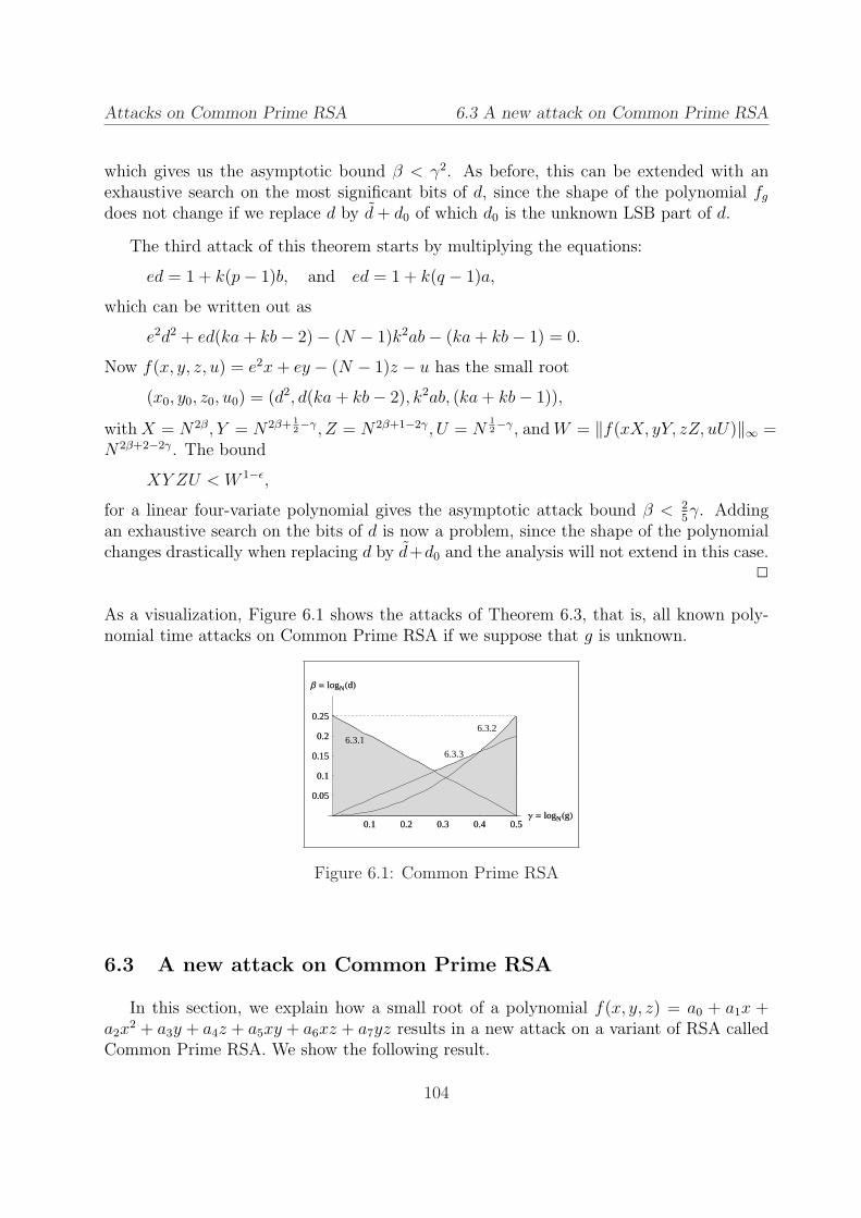
Attacks on Common Prime RSA 6.3 A new attack on Common Prime RSA
which gives us the asymptotic bound β < γ2. As before, this can be extended with anexhaustive search on the most significant bits of d, since the shape of the polynomial fg
does not change if we replace d by d + d0 of which d0 is the unknown LSB part of d.
The third attack of this theorem starts by multiplying the equations:
ed = 1 + k(p− 1)b, and ed = 1 + k(q − 1)a,
which can be written out as
e2d2 + ed(ka + kb− 2)− (N − 1)k2ab− (ka + kb− 1) = 0.
Now f(x, y, z, u) = e2x + ey − (N − 1)z − u has the small root
(x0, y0, z0, u0) = (d2, d(ka + kb− 2), k2ab, (ka + kb− 1)),
with X = N2β, Y = N2β+ 12−γ, Z = N2β+1−2γ, U = N
12−γ, and W = ‖f(xX, yY, zZ, uU)‖∞ =
N2β+2−2γ. The bound
XY ZU < W 1−ε,
for a linear four-variate polynomial gives the asymptotic attack bound β < 25γ. Adding
an exhaustive search on the bits of d is now a problem, since the shape of the polynomialchanges drastically when replacing d by d+d0 and the analysis will not extend in this case.
2
As a visualization, Figure 6.1 shows the attacks of Theorem 6.3, that is, all known poly-nomial time attacks on Common Prime RSA if we suppose that g is unknown.
0.1 0.2 0.3 0.4 0.5Γ = logNHgL
0.05
0.1
0.15
0.2
0.25
Β = logNHdL
6.3.16.3.2
6.3.3
0.1 0.2 0.3 0.4 0.5Γ = logNHgL
0.05
0.1
0.15
0.2
0.25
Β = logNHdL
Figure 6.1: Common Prime RSA
6.3 A new attack on Common Prime RSA
In this section, we explain how a small root of a polynomial f(x, y, z) = a0 + a1x +a2x
2 + a3y + a4z + a5xy + a6xz + a7yz results in a new attack on a variant of RSA calledCommon Prime RSA. We show the following result.
104

Attacks on Common Prime RSA 6.3 A new attack on Common Prime RSA
Theorem 6.4 (Attack on Common Prime RSA)Under Assumption 3.7, for every ε > 0, there exists n0 such that for every n > n0, thefollowing holds: Let N = pq be an n-bit RSA modulus, and p, q primes of bitsize 1
2n such
that p − 1 = 2ga and q − 1 = 2gb, for some prime g of bitsize γn, with 0 ≤ γ < 12. Let
ed ≡ 1 mod 2gab, with bitsize(e) = (1 − γ)n and bitsize(d) = βn, with 0 < β < 1 − γ.Then d can be found in time polynomial in n provided that
β <1
4(4 + 4γ −
√13 + 20γ + 4γ2)− ε.
6.3.1 Description of the new attack
The new attack can be obtained by treating the equation in Hinek’s second lattice attack(Theorem 6.3.3) in a different way. We will now show how to modify Hinek’s attack toobtain the result of Theorem 6.4.
Proof of Theorem 6.4:
Let us take another look at the equation
e2d2 + ed(ka + kb− 2)− (ka + kb− 1)− (N − 1)k2ab = 0,
in which the unknowns are d, k, a and b. We can conclude from this equation that thepolynomial f(x, y, z) = e2x2 + ex(y + z − 2) − (y + z − 1) − (N − 1)yz has a small root
(d, ka, kb) with X = Nβ, Y = Nβ+ 12−γ, Z = Nβ+ 1
2−γ. Moreover, W = N2+2β−2γ.
Note that the polynomial involved in this attack has the same set of monomials as thepolynomial of the attack on CRT-Qiao&Lam (see Section 5.4.1). Therefore, we can usethe asymptotical bound
X7+9τ+3τ2
(Y Z)5+ 92τ < W 3+3τ
which yields
3βτ 2 + 3(4β − 1
2− γ)τ + (11β − 1− 4γ) < 0.
For the optimal value of τ , namely τ =12+γ−4β
2β, this reduces to
β <1
4(4 + 4γ −
√13 + 20γ + 4γ2).
Figure 6.2 shows the new attack region as well as the known attacks, for any size ofmodulus N . Combinations of d and g that should be considered unsafe by the new attackare in the dark shaded area, whereas the lighter shaded area was already unsafe by theknown attacks. It can be seen that the number of ‘safe’ combinations {d, g} with d < N
14
has significantly decreased.
105

Attacks on Common Prime RSA 6.3 A new attack on Common Prime RSA
0.1 0.2 0.3 0.4 0.5Γ =logNHgL
0.05
0.1
0.15
0.2
0.25
Β = logNHdL
known attacks
new attack
0.1 0.2 0.3 0.4 0.5Γ =logNHgL
0.05
0.1
0.15
0.2
0.25
Β = logNHdL
Figure 6.2: New attack region
We note that for ‘small’ N (such as the regular 1024 bits), other attacks such as factoringattacks may apply, see [32]. Also, depending on the size of N , the attacks in the figurecould be extended by an additional exhaustive search.
6.3.2 Experiments for the new attack
We performed experiments to check the validity of Assumption 3.7 and to demonstrate thepracticality of our attack. We have implemented the new attack for the parameter settingm = 2, t = 0 (without the possible additional exhaustive search), to give an impression onwhat a realistic bound is for the smallest lattice possible. Of course, extending to m = 3,m = 4, etc. and using x-shifts will give results closer to the theoretical attack bound
β <1
4(4 + 4γ −
√13 + 20γ + 4γ2),
but will also result in a longer time needed for the lattice basis reduction. For m = 2, t = 0the reduction time (the longest part of the attack) is about one minute. The followingtable summarizes the experimental results performed for n = 1024. As one can see, theresults are already outside the asymptotical range of the known attacks.
maximal β obtained β maximal βγ (asymptotic) (m = 2, t = 0) (asymptotic)
new attack new attack known attacks0.10 0.130 0.07 0.200.20 0.164 0.10 0.150.30 0.200 0.13 (∗) 0.120.40 0.237 0.17 (∗) 0.160.50 0.275 0.2 0.25
Table 6.1: Experiments for the new attack on Common Prime RSA
106

Attacks on Common Prime RSA 6.4 Tabular overview
The resultant heuristic of Assumption 3.7 worked perfectly in most cases. However, inthe rare situation that both β and γ were very small (e.g. γ = 0.1 and β = 0.05), weencountered cases where some of the polynomials ri were algebraically dependent. Inthese cases, we could still recover the secret information in two different ways. One waywas to use combinations of r1 and the somewhat ‘larger’ ri for i > 2, instead of onlyr1 and r2. The other way was by examining the cause of the zero resultant. In essence,Resy(Resx(r1, f), Resx(r2, f)) = 0 because Resx(r1, f) and Resx(r2, f) have a common poly-nomial factor, whose coefficients immediately reveal the secrets.
6.4 Tabular overview
The following table shows the known polynomial time attacks on Common Prime RSA.
Type of attack Attack bound Reference
known g γ ≥ 14
Thm. 6.1
known g and β < 76− 5
3γ − 1
3
√(7− 10γ)(1− 4γ)− ε and γ < 1
4Thm. 6.2
small d
unknown g and β < 14− 1
2γ Thm. 6.3.1
small dβ < γ2 − ε Thm. 6.3.2
β < 25γ − ε Thm. 6.3.3
β < 14(4 + 4γ −
√13 + 20γ + 4γ2)− ε Thm. 6.4
Table 6.2: Polynomial time attacks on Common Prime RSA
107

7Conclusion & open questions
7.1 The security of RSA: Advice for implementors
In this thesis we have presented many variants on RSA, and discussed a variety of attackson them. In this section we give a conclusion on the security of RSA, and on the possibilitiesto speed up RSA encryption or decryption by choosing special parameters.
First of all, the main lesson of this thesis is:
One should be very careful in choosing special relations between RSA parameters.
Although these special relations may lead to more efficient RSA variants, they also givemore possibilities to the attacker. Hence, the safest thing to do is to follow a standardimplementation (for an n-bit modulus N that is the product of two primes):
• Choose a parameter n such that you are certain that factoring an n-bit RSA moduluscannot be performed.
• Choose random 12n-bit primes p and q independently.
If p and q are truly chosen at random, then one can expect that p − q is not smallenough to apply one of the attacks described by de Weger [74], but a check can alwaysbe performed. Similarly, one could check that gcd(p − 1, q − 1) is not too large, toprevent attacks on the Common Prime RSA variant.
• Choose a random integer e smaller than, and coprime to φ(N) = (p− 1)(q − 1).If e is chosen at random then one can expect with overwhelming probability that ithas the same bitsize as φ(N) (or only a few bits smaller), so attacks on small e willnot apply.
• Determine d by applying the Extended Euclidean Algorithm on e and φ(N).Again, one can expect that d is ‘full size’, hence attacks on small d do not apply.
• In order to use Quisquater/Couvreur’s decryption method using the Chinese Remain-der Theorem [61], compute dp ≡ d mod (p− 1) and dq ≡ d mod (q − 1).In this way, dp and dq will have bitsize 1
2n, so attacks on small dp, dq will not apply.
108

Conclusion & open questions 7.1 The security of RSA: Advice for implementors
In the above steps it is very easy to perform tests to check if e, d, and dp, dq are indeed ofthe expected bitsize.
Specific applications may ask for more efficient variants, so let us discuss the possibili-ties for speeding up RSA that have been treated in this thesis.
RSA-Small-e and RSA-CRT-Small-e:
One of the most popular RSA variants in practice is RSA with a small public exponent e(or RSA-CRT with a small e). The choice e = 3 should be considered unsafe nowadays.For e = 3, there are simply too many things that can go wrong, like:
• attacks involving specific intercepted ciphertexts (Section 2.3),
• attacks related to the implementation (Section 2.3),
• partial key exposure attacks (Section 4.2 and 5.2).
For larger e, like the popular e = 65537, the only concern is partial key exposure attacks.As has been known for some time (see Section 4.2), if e is this small, then only 1
4n LSBs of
the decryption exponent d are sufficient to retrieve the factorization of N . Similarly, only14n LSBs or 1
4n MSBs of dp are sufficient if RSA-CRT-Small-e is used for a very small value
of e.Even for larger e, one must always be aware that partial key exposure attacks exist
(see Chapter 4) and that it is essential to keep all bits of d (or dp, dq) secret, e.g. takecountermeasures against side channel attacks.
RSA-Small-d and RSA-CRT-Small-dp, dq:
If one wants to decrease the cost for RSA decryption (or RSA signature generation), thenthe main possibilities are to use RSA-Small-d or RSA-CRT-Small-dp, dq. Since the attacksof Wiener [75] and Boneh/Durfee [10] we know that there exists a polynomial time attackwhenever d < N0.292.
In their paper, Boneh and Durfee explain that for d < N0.5, the equation
x(N + 1− y) ≡ 1 mod e
is likely to have a unique solution x = k, y = p + q. Therefore, they propose to choosed > N0.5. In all parameter proposals, it is wise to choose your parameters ‘at a safedistance’ from the current attacks. Having a list of attacks simply does not guarantee thenon-existence of other attacks.
When choosing a small d, one again has to keep in mind that partial key exposureattacks exist whenever d is less than n bits long. Hence, sufficient countermeasures mustbe taken such that parts of the secret key cannot leak.
For the case of small dp, dq, note that in this thesis, the first polynomial time attack onRSA-Small-dp, dq is discussed. However, the bound {dp, dq} < N0.0734 is hard to achieve inpractice, and we think that {dp, dq} > N0.25 is still a very safe choice that can be made.
109

Conclusion & open questions 7.2 Open questions
RSA-CRT-UnbalancedPrimes and RSA-CRT-BalancedExponents:
We doubt that the CRT-UnbalancedPrimes and CRT-BalancedExponents variants areused in practice. Especially the CRT-UnbalancedPrimes setting was mainly proposedin [52] to investigate which CRT-variants could be attacked in polynomial time. The CRT-BalancedExponents variant has a better motivation, but seems to give rise to many attacks.If one wants to use one of these variants, then we recommend to choose the parameters ‘ata safe distance’ from the current attacks (see Figure 5.1 and 5.3). For instance a suitablechoice for CRT-BalancedExponents could be e ≈ Nα and {dp, dq} ≈ Nβ with α > 1
2and
β > 34− 1
2α. However, since we do not know how to efficiently generate key pairs that
satisfy this constraint (see Section 2.2), the relevance of this variant is truly questionable.
Other variants:
We do not recommend to use Common Prime RSA. Apart from the polynomial timeattacks in Section 6 there are other, non-polynomial time time attacks that are alreadypretty powerful for n = 1024 or n = 2048 (see [32]). For these choices of n, there is simplynot enough room to choose d < N0.25 at some safe distance from the known attacks.
At this moment CRT-Qiao&Lam seems to be secure for dp > N0.25, but (as is the casefor all variants) other attacks may arise that improve the current attack bound.
Naturally, we have not discussed all RSA variants in detail (although we have coveredthe most popular variants). Since Multi-prime RSA and Takagi’s RSA were not discussedin this work, we refer to [33] and [13, 55] for the known attacks on these variants.
7.2 Open questions
In this section, we discuss some interesting open questions related to the work in this thesis.First, we will describe two open questions related to finding small roots of polynomials.Afterwards, we discuss two open questions related to cryptanalysis.
Open questions related to finding small roots:
Refinements of the (extended) strategy to choose shift polynomials:
In Section 3.3, we discussed a general strategy to choose the shift polynomials used in aCoppersmith method given the monomials that appear in a polynomial fN or f . For theextended strategy, we noted that in some cases, it is profitable to use extra shifts of acertain variable (or certain variables). Hence, the current way of choosing the shifts is touse the basic strategy, and then trying out some possibilities for using extra shifts.
Open question: Can we find a refinement of the way to choose the shift polynomials thatguarantees an optimal bound for any polynomial f that the strategy is used on?
110

Conclusion & open questions 7.2 Open questions
Investigating the heuristic involved when dealing with multivariate polynomials:
Recall that in Coppersmith methods for finding roots of multivariate polynomials, we oftenhave to deal with a heuristic assumption. If we want to find a modular root of a polynomialfN in v variables (v ≥ 2), and the LLL reduction gives us polynomials r1, r2, . . . , rv thatshare the desired root over the integers, then we can extract the root assuming that the ri
are algebraically independent. In the case of finding a small integer root of a polynomialf in v variables (v ≥ 3), if the LLL reduction gives us polynomials r1, r2, . . . , rv−1 thatshare the desired root over the integers, then we can extract the root assuming that thepolynomials of the set {f, r1, . . . , rv−1} are algebraically independent. The validation ofsuch an assumption is done using experiments, and since usually no problems occur, most(practically oriented) researchers see no problems in using a heuristic attack. However, forthe theory of Coppersmith methods it is important to study this heuristic in more detail.
Open question: Can we define in which cases a Coppersmith method for a multivariatepolynomial is provable, in other words, does not rely on a heuristic assumption?
Recently, Bauer and Joux [2] made some important progress in this area. For the caseof finding small roots of integer polynomials f(x, y, z) they use the traditional Copper-smith method to find a polynomial r1(x, y, z) independent of f that also has the desiredroot. Next, they construct a new lattice similar to Coppersmith’s one that produces a thirdpolynomial r2(x, y, z) that contains the root and that is independent from {f, r1}. Bauerand Joux show that if a certain criterion on the Grobner basis of the ideal defined by {f, r1}is satisfied, their method for finding a third independent polynomial r2 will always succeed.
Open questions related to cryptanalysis:
Extending attacks with an exhaustive search:
On the one hand, we have seen in this thesis that for a given attack using a Coppersmithmethod, it can be costly to perform an attack in practice for parameters that are close tothe attack bound. On the other hand, in most cases an attack bound can be extended alittle bit by adding an exhaustive search.
Let us discuss a small example. Recall the new attack on Common Prime RSA ofSection 6.3.1. We obtained the asymptotical bound
X7+9τ+3τ2
(Y Z)5+ 92τ < W 3+3τ , for
X = |d| = Nβ,
Y = |ka| = Nβ+ 12−γ,
Z = |kb| = Nβ+ 12−γ,
W = max{e2X2, (N − 1)Y Z} = N2+2β−2γ.
Now suppose we guess a number of most significant bits of d (say, a string of bitsize µn,for some 0 < µ < β). Then we can use the same asymptotical bound, but now with
X = Nβ−µ, Y = Z = Nβ+ 12−γ, W = N2+2β−2γ.
111

Conclusion & open questions 7.2 Open questions
One can check that, instead of the asymptotical attack bound
β <1
4(4 + 4γ −
√13 + 20γ + 4γ2)
we now obtain
β <1
4(4 + 4γ −
√13 + 20γ + 4γ2 − 20µ− 8γµ + 4µ2).
A typical example would be γ = 0.1, µ = 0.02 (think of µ = 0.02 as guessing about 20 bitsof d if N is a 1024-bit modulus). Then, the normal asymptotic bound of the attack is
β < 0.130464,
whereas the asymptotic bound with µ = 0.02 is
β < 0.143914.
Hence, by taking µ = 0.02 you achieve an improvement of the attack bound by 0.01345. Itfollows that one cannot directly translate the knowledge of 20 bits into an improvement ofthe attack bound by 20 bits. In other words, if one would perform this attack 220 times foreach possibility of the 20 MSBs of d, then one still would not be able to handle a d thatexceeds the asymptotical bound by 20 bits. This brings us to our open question.
Open question: Is there a better way to combine an attack using a Coppersmith methodwith an exhaustive search?
Imagine that if d(1)M and d
(2)M are two possibilities for the MSBs of d, and that d
(1)M and
d(2)M are almost the same. Then is it really necessary to perform Coppersmith’s method
twice? The lattices involved will be very similar and it seems like a waste of computingtime to perform the LLL reduction of these slightly different lattices twice. Is it possibleto reuse a method performed for one candidate dM for a number of other candidates d′Mthat are ‘close enough’ to dM?
Refining attack bounds using sublattices:
An important facet of Coppersmith attacks on RSA that we have not yet discussed in thisthesis, is the use of sublattices. Boneh and Durfee [10] were the first to use sublattices toimprove an attack bound. In Section 3.3.1 we explained that using the extended strategyfor finding small modular roots, one can find the factorization of N in polynomial time ifd < N0.284. However, the improved attack bound that Boneh and Durfee give is d < N0.292.Let us briefly sketch how the use of sublattices helps here.
Recall the example given in Section 3.3.1 for the Boneh/Durfee-attack for the case{m = 2, t = 1}, where the lattice L was spanned by the rows of a 9 × 9 matrix. Nowimagine that one looks at a lattice L′ that is spanned by a subset of these nine shiftpolynomials. That means that the lattice L′ does not have full rank anymore, so calculating
112

Conclusion & open questions 7.2 Open questions
its determinant (or, as it should be called in this case, its volume) takes more effort.However, “throwing away” some of the rows can result in a better bound, as shown in [10].
Often, the experiments of an attack will indicate that using a sublattice can be profi-table. In practice, the smallest lattice vectors of the LLL reduced basis turn out to be aninteger linear combination of only a specific subset of the original shift polynomials. Inother words, the LLL algorithm does not use all vectors to approximate the shortest latticevectors. This suggests that analyzing the attack for the lattice L′ containing only this sub-set of the shift polynomials can lead to an improved attack bound. For more details, werefer to the papers of Boneh/Durfee and Blomer/May on this topic [10, 5].
In our new attacks on RSA variants, we occasionally encountered this phenomenon.Recall the result of Theorem 5.9, our new attack on CRT-Small-dp, dq. As we mentioned inSection 5.3.3, we used Coppersmith’s original method for the experiments, to profit fromthe fact that the lattices that need to be reduced in Coppersmith’s original method havesmaller dimension than the ones in Coron’s reformulation [18]. However, with Copper-smith’s original approach it is harder to analyze if sublattices can improve the attackbound. Recall that in Coron’s method, the shortest vectors in the reduced method imme-diately correspond to the small polynomials ri. Hence the transformation matrix of theLLL reduction can tell us which shift polynomials have contributed to the smallest poly-nomials ri. We have programmed our new attack on RSA-CRT using Coron’s method for{m = 2, t = 1} (a 81-dim. lattice) to see what would happen in the LLL process. It turnsout that the polynomials ri(x1, x2, x3, x4) corresponding to the smallest vectors in the LLLreduced basis all have a special structure.
In the following description of these polynomials ri we have replaced X2 by X1 and X4
by X3, since the upper bounds that we have for x(0)1 = dp and x
(0)2 = dq are the same, as
are the upper bounds for x(0)3 = kp and x
(0)4 = kq.
ri(x1, x2, x3, x4) := a1X41X
23 · f + a2X
31X
23 · (x1 + x2) · f + a3X
41X3 · (x3 + x4) · f
+ a4X31X3 · (x1x4 + x2x3) · f + a5X
21X
23 · x1x2 · f +
+ a6X41 · x3x4 · f + a7X
21X
23 · (x2
1 + x22) · f +
+ a8X31X3 · (x1x3 + x2x4) · f + a9X
21X3 · (x2
1x4 + x22x3) · f
+ a10X21X3 · (x1x2x3 + x1x2x4) · f + a11X1X
23 · (x2
1x2 + x1x22) · f
+ a12X31 · (x1x3x4 + x2x3x4) · f + a13X
21 · x1x2x3x4 · f
+ a14X1X3 · (x21x2x4 + x1x
22x3) · f + a15X
23 · (x2
1x22) · f
−⌊
sum of coefficients of x23 in the above polynomials
WX41X2
3
⌉WX4
1X23 · x2
3
− . . .
−⌊
sum of coefficients of x31x
32 in the above polynomials
WX41X2
3
⌉WX4
1X23 · x3
1x32.
113

Conclusion & open questions 7.2 Open questions
Two plain observations are:
• Due to the symmetry of
f(x1, x2, x3, x4) := (ex1 + x3 − 1)(ex2 + x4 − 1)−Nx3x4
= e2x1x2 + e(x1x4 + x2x3 − x1 − x2) + (1−N)x3x4 − x3 − x4 + 1,
the polynomials corresponding to the smallest vectors are also very symmetrical.
• The rows corresponding to the polynomials
Rx23, Rx2x
23, Rx2
3x4, Rx24, Rx1x
24, Rx3x
24, Rx2
1x24, Rx2
2x23, Rx1x
23, Rx2x
24,
are not used in the smallest vectors. This is because the term⌊
sum of coefficients of x23 in the above polynomials
WX41X
23
⌉
is zero, and equivalently for x2x23, . . . , x2x
24.
Whether or not these observations can be used to obtain a better attack bound, is theopen question with which we conclude this thesis.
Open question: Can we use the fact that the ‘smallest’ polynomials are symmetrical, andthat a few rows of the original matrix are not necessary for LLL to create these ‘small’polynomials, to improve the attack bound on CRT-Small-dp, dq?
A possible direction to take in order to answer this question is to look at the followingsublattice of L. Replace the two rows that represent the shifts polynomials
x1 · f ·X(m−1)+t−11 X
(m−1)+t2 Xm−1
3 Xm−14 and x2 · f ·X(m−1)+t
1 X(m−1)+t−12 Xm−1
3 Xm−14
by one row that contains their sum. Since we know that the shortest vectors in the LLLreduced basis take the shifts of x1 and x2 with the same coefficient, the sum of the twoshifts can be used instead of two single shifts. The same holds for the shifts of x3 and x4,the shifts of x1x4 and x2x3, etc. All of these couples of shifts can be replaced by their sum.
In the example we gave for the new RSA-CRT-Small-dp, dq attack (for m = 2, t = 1),our sublattice L′ looks like:
shift 1 : f ·X41X
23 ,
shift 2 : (x1 + x2) · f ·X31X
23 ,
shift 3 : (x3 + x4) · f ·X41X
23 ,
. . .shift 14 : (x2
1x2x4 + x1x22x3) · f ·X1X3,
shift 15 : x21x
22 · f ·X2
3 ,
114

Conclusion & open questions 7.2 Open questions
together with the rows for the monomials that are in M\S:
shift 16 : (x23 + x2
4)R,shift 17 : (x2x
23 + x1x
24)R,
shift 18 : (x23x4 + x3x
24)R,
. . .shift 44 : (x3
1x22x4 + x2
1x32x3)R,
shift 45 : x31x
32R.
In this example, the lattice L′ is defined by 45 polynomials with in total 81 monomials.The short vectors of L that were found by the LLL reduction are also in L′. In thisspecific case, we even know that we can eliminate five rows more because we know thatthe shifts (x2
3 + x24)RX4
1 , etc. do not appear in the smallest reduced lattice vectors of L.The determinant of the 45-dimensional L′ of the example is given by
det(L′) = 218(X1X2)128(X3X4)
74W 30, so (det(L′))145 ≈ (X1X2)
2.844(X3X4)1.644W 0.667.
This is only slightly smaller than the value of
(det(L))181 = (X1X2)
23281 (X3X4)
13481 W
5681 ≈ (X1X2)
2.864(X3X4)1.654W 0.691.
Substituting the values of the Xi, W , and R in the respective inequalities det(L′)145 < R
and det(L)181 < R yields the bounds β < 0.0096 and β < −0.0153.
The determinant of the 40-dimensional lattice L′′ is a more complicated expression thatinvolves many terms in the Xi, W , e and N . When we substitute all known values in asimplified version of the expression det(L′′)
140 < R, we find the bound β < 0.0102. This
bound is supported by the experiments in Section 5.3.4, where we can see in Table 5.3that for {m = 2, t = 1}, we can successfully mount an attack if the length of the privateCRT-exponents is about 1
100n.
At this moment, it is not yet clear if and how well this approach would work in general(especially for m →∞ with optimal t). We do not have a general analysis of the determi-nant of the lattice L′ (which does not have full rank anymore, so this determinant is thevolume of the lattice). Trying this and other approaches to improve the attack bound ofRSA-CRT-Small-dp, dq will be one of the many challenges in the fascinating research areaof cryptanalysis of RSA variants using small roots of polynomials.
115

Bibliography
[1] A. Baker and H. Davenport. The equations 3x2− 2 = y2 and 8x2− 7 = z2. QuarterlyJournal of Mathematics (Oxford) (2), volume 20: pages 129–137, 1969.
[2] A. Bauer and A. Joux. Toward a rigorous variation of Coppersmith’s algorithm onthree variables. In Proceedings of Eurocrypt’07, volume 4515 of Lecture Notes inComputer Science, pages 361–378, 2007.
[3] D. Bleichenbacher. Chosen ciphertext attacks against protocols based on the RSAencryption standard PKCS #1. In Proceedings of Crypto’98, volume 1462 of LectureNotes in Computer Science, pages 1–12, 1998.
[4] D. Bleichenbacher and A. May. New attacks on RSA with small secret CRT-exponents.In Proceedings of PKC’06, volume 3958 of Lecture Notes in Computer Science, pages1–13, 2006.
[5] J. Blomer and A. May. Low secret exponent RSA revisited. In Proceedings of CaLC’01,volume 2146 of Lecture Notes in Computer Science, pages 4–19, 2001.
[6] J. Blomer and A. May. New partial key exposure attacks on RSA. In Proceedings ofCrypto’03, volume 2729 of Lecture Notes in Computer Science, pages 27–43, 2003.
[7] J. Blomer and A. May. A tool kit for finding small roots of bivariate polynomialsover the integers. In Proceedings of Eurocrypt’05, volume 3494 of Lecture Notes inComputer Science, pages 251–267, 2005.
[8] D. Boneh. Twenty years of attacks on the RSA cryptosystem. Notices of the AMS,volume 46(2): pages 203–213, 1999.
[9] D. Boneh, R.A. DeMillo, and R.J. Lipton. On the importance of checking crypto-graphic protocols for faults. In Proceedings of Eurocrypt’97, volume 1233 of LectureNotes in Computer Science, pages 37–51, 1997.
[10] D. Boneh and G. Durfee. Cryptanalysis of RSA with private key d less than N 0.292.IEEE Transactions on Information Theory, volume 46(4): pages 1339–1349, 2000.
[11] D. Boneh, G. Durfee, and Y. Frankel. Exposing an RSA private key given a smallfraction of its bits, full version of [12]. http://crypto.stanford.edu/∼dabo/abstracts/bits of d.html.
[12] D. Boneh, G. Durfee, and Y. Frankel. Exposing an RSA private key given a smallfraction of its bits. In Proceedings of Asiacrypt’98, volume 1514 of Lecture Notes inComputer Science, pages 25–34, 1998.
116
[13] D. Boneh, G. Durfee, and N. Howgrave-Graham. Factoring n = prq for large r. InProceedings of Crypto’99, volume 1666 of Lecture Notes in Computer Science, pages326–337, 1999.
[14] D. Coppersmith. Finding a small root of a bivariate integer equation; factoring withhigh bits known. In Proceedings of Eurocrypt’96, volume 1070 of Lecture Notes inComputer Science, pages 178–189, 1996.
[15] D. Coppersmith. Finding a small root of a univariate modular equation. In Proceedingsof Eurocrypt’96, volume 1070 of Lecture Notes in Computer Science, pages 155–165,1996.
[16] D. Coppersmith. Small solutions to polynomial equations, and low exponent RSAvulnerabilities. Journal of Cryptology, volume 10(4): pages 233–260, 1997.
[17] D. Coppersmith, M. Franklin, J. Patarin, and M. Reiter. Low exponent RSA withrelated messages. In Proceedings of Eurocrypt’96, volume 1070 of Lecture Notes inComputer Science, pages 1–9, 1996.
[18] J.-S. Coron. Finding small roots of bivariate integer polynomial equations revisited.In Proceedings of Eurocrypt’04, volume 3027 of Lecture Notes in Computer Science,pages 492–505, 2004.
[19] J.-S. Coron. Finding small roots of bivariate integer polynomial equations: a directapproach. In Proceedings of Crypto’07, volume 4622 of Lecture Notes in ComputerScience, 2007.
[20] J.-S. Coron and A. May. Deterministic polynomial-time equivalence of computing theRSA secret key and factoring. Journal of Cryptology, 20: pages 39–50, 2007.
[21] D. Cox, J. Little, and D. O’Shea. Ideals, varieties, and algorithms. An introductionto computational algebraic geometry and commutative algebra. Undergraduate textsin mathematics. Springer, 1992.
[22] J.-F. Dhem, F. Koeune, P.-A. Leroux, P. Mestre, J.-J. Quisquater, and J.-L. Willems.A practical implementation of the timing attack. In Proceedings of CARDIS’98,volume 1820 of Lecture Notes in Computer Science, pages 167–182, 1998.
[23] W. Diffie and M. Hellman. New directions in cryptography. IEEE Transactions onInformation Theory, volume 22(6): pages 644–654, 1976.
[24] ECRYPT-AZTEC. Hardness of the main computational problems used in cryptogra-phy. IST-2002-507932, http://www.ecrypt.eu.org/documents/D.AZTEC.4-1.1.pdf.
[25] M. Ernst, E. Jochemsz, A. May, and B.M.M. de Weger. Partial key exposure attackson RSA up to full size exponents. In Proceedings of Eurocrypt’05, volume 3494 ofLecture Notes in Computer Science, pages 371–386, 2005.
117

[26] J.-C. Faugere. A new efficient algorithm for computing Grobner bases. Journal ofPure and Applied Algebra, 139: pages 61–88, 1999.
[27] S.D. Galbraith, C. Heneghan, and J.F. McKee. Tunable balancing of RSA, full versionof [28]. http://www.isg.rhul.ac.uk/∼sdg/full-tunable-rsa.pdf.
[28] S.D. Galbraith, C. Heneghan, and J.F. McKee. Tunable balancing of RSA. In Proceed-ings of ACISP’05, volume 3574 of Lecture Notes in Computer Science, pages 280–292,2005.
[29] K.O. Geddes, S.R. Czapor, and G. Labahn. Algorithms for computer algebra. KluwerAcademic Publishers, 1992.
[30] G.H. Hardy and E.M. Wright. An introduction to the theory of numbers. OxfordUniversity Press, 1979.
[31] J. Hastad. Solving simultaneous modular equations of low degree. SIAM Journal onComputing, volume 17(2): pages 336–341, 1988.
[32] M.J. Hinek. Another look at small RSA exponents. In Proceedings of CT-RSA’06,volume 3860 of Lecture Notes in Computer Science, pages 82–98, 2006.
[33] M.J. Hinek. On the security of multi-prime RSA. Technical report, CACR, 2006.
[34] M.J. Hinek and Douglas R. Stinson. An inequality about factors of multivariatepolynomials. Technical report, CACR, 2006.
[35] N. Howgrave-Graham. Finding small roots of univariate modular equations revisited.In Proceedings of IMA Int. Conf., volume 1355 of Lecture Notes in Computer Science,pages 131–142, 1997.
[36] E. Jochemsz and B.M.M. de Weger. A partial key exposure attack on RSA usinga 2-dimensional lattice. In Proceedings of ISC’06, volume 4176 of Lecture Notes inComputer Science, pages 203–216, 2006.
[37] E. Jochemsz and A. May. A strategy for finding roots of multivariate polynomials withnew applications in attacking RSA variants. In Proceedings of Asiacrypt’06, volume4284 of Lecture Notes in Computer Science, pages 267–282, 2006.
[38] E. Jochemsz and A. May. A polynomial time attack on RSA with private CRT-exponents smaller than N 0.073. In Proceedings of Crypto’07, volume 4622 of LectureNotes in Computer Science, 2007.
[39] A. Joux and F. Olivier. Side-channel analysis. In Encyclopedia of Cryptography andSecurity, pages 571–576. Springer, 2005.
118

[40] C.S. Jutla. On finding small solutions of modular multivariate polynomial equations.In Proceedings of Eurocrypt’98, volume 1403 of Lecture Notes in Computer Science,pages 158–170, 1998.
[41] D. Kahn. The codebreakers: the story of secret writing. MacMillan, 1967.
[42] P.C. Kocher. Timing attacks on implementations of Diffie-Hellman, RSA, DSS, andother systems. In Proceedings of Crypto’96, volume 1109 of Lecture Notes in ComputerScience, pages 104–113, 1996.
[43] P.C. Kocher, J. Jaffe, and B. Jun. Differential power analysis. In Proceedings ofCrypto’99, volume 1666 of Lecture Notes in Computer Science, pages 388–397, 1999.
[44] J.L. Lagrange. Recherches d’arithmetique. Nouveaux Memoires de l’Academie Royaledes Sciences et des Belles Lettres de Berlin, 1773.
[45] A.-M. Legendre. Essai sur la theorie des nombres. Duprat, Paris, An VI, 1798.
[46] A.K. Lenstra. Integer factoring. In Encyclopedia of Cryptography and Security, pages290–297. Springer, 2005.
[47] A.K. Lenstra and H.W. Lenstra Jr. (eds.). The development of the number field sieve.Lecture Notes in Mathematics, volume 1554, 1993.
[48] A.K. Lenstra, H.W. Lenstra Jr., and L. Lovasz. Factoring polynomials with rationalcoefficients. Mathematische Annalen, volume 261(4): pages 515–534, 1982.
[49] H.W. Lenstra Jr. Factoring integers with elliptic curves. Annals of Mathematics,volume 126(2): pages 649–673, 1987.
[50] C.H. Lim and P.J. Lee. Security and performance of server-aided RSA computationprotocols. In Proceedings of Crypto’95, volume 963 of Lecture Notes in ComputerScience, pages 70–83, 1995.
[51] A. May. RSA & meet-in-the-middle Angriffe. Chapter from the course “PublicKey Kryptanalyse”, available via http://www.informatik.tu-darmstadt.de/KP/lehre/ws0506/vl/pkk.html.
[52] A. May. Cryptanalysis of unbalanced RSA with small CRT-exponent. In Proceedingsof Crypto’02, volume 2442 of Lecture Notes in Computer Science, pages 242–256, 2002.
[53] A. May. New RSA Vulnerabilities Using Lattice Reduction Methods. PhD thesis,University of Paderborn, 2003.
[54] A. May. Computing the RSA secret key is deterministic polynomial time equivalentto factoring. In Proceedings of Crypto’04, volume 3152 of Lecture Notes in ComputerScience, pages 213–219, 2004.
119
[55] A. May. Secret exponent attacks on RSA-type schemes with moduli prq. In Proceedingsof PKC’04, volume 2947 of Lecture Notes in Computer Science, pages 218–230, 2004.
[56] J.F. McKee and R. Pinch. Further attacks on server-aided RSA cryptosystems.http://citeseer.ist.psu.edu/388295.html, 1998.
[57] H. Minkowski. Geometrie der Zahlen. Teubner Verlag, 1896.
[58] P.Q. Nguyen and D. Stehle. Floating-point LLL revisited. In Proceedings of Euro-crypt’05, volume 3494 of Lecture Notes in Computer Science, pages 215–233, 2005.
[59] P.Q. Nguyen and J. Stern. The two faces of lattices in cryptology. In Proceedings ofCaLC’01, volume 2146 of Lecture Notes in Computer Science, pages 146–180, 2001.
[60] G. Qiao and K.-Y. Lam. RSA signature algorithm for microcontroller implementation.In Proceedings of CARDIS’98, volume 1820 of Lecture Notes in Computer Science,pages 353–356, 1998.
[61] J.-J. Quisquater and C. Couvreur. Fast decipherment algorithm for RSA public-keycryptosystem. Electronic Letters, volume 18: pages 905–907, 1982.
[62] J.-J. Quisquater and F. Koeune. Side channel attacks, state of the art. Available viahttp://www.crypto.rub.de/en sclounge.html, 2002.
[63] D. Redmond. Number theory: an introduction, volume no. 201 of Monographs andTextbooks in Pure and Applied Mathematics. Marcel Dekker, 1996.
[64] R. Rivest, A. Shamir, and L. Adleman. A method for obtaining digital signaturesand public-key cryptosystems. Communications of the ACM, volume 21(2): pages120–126, 1978.
[65] W. Scharlau and H. Opolka. From Fermat to Minkowski. Lectures on the theoryof numbers and its historical development. Undergraduate texts in mathematics.Springer-Verlag, 1985.
[66] V. Shoup. NTL: A library for doing number theory. http://www.shoup.net/ntl.
[67] S. Singh. The code book: the science of secrecy from ancient Eqypt to quantum cryp-tography. Anchor books, 2000.
[68] R. Steinfeld and Y. Zheng. An advantage of low-exponent RSA with modulus primessharing least significant bits. In Proceedings of CT-RSA’01, volume 2020 of LectureNotes in Computer Science, pages 52–62, 2001.
[69] H.-M. Sun, M.J. Hinek, and M.-E. Wu. On the design of rebalanced RSA-CRT, revisedversion of [70]. Technical report, CACR, 2005.
120
[70] H.-M. Sun and M.-E. Wu. An approach towards RSA-CRT with short public exponent.http://eprint.iacr.org/2005/053, 2005.
[71] T. Takagi. Fast RSA-type cryptosystem modulo pkq. In Proceedings of Crypto’98,volume 1462 of Lecture Notes in Computer Science, pages 318–326, 1998.
[72] E.R. Verheul and H.C.A. van Tilborg. Cryptanalysis of ’less short’ RSA secret ex-ponents. Applicable Algebra in Engineering Communication and Computing, volume8(5): pages 425–435, 1997.
[73] P.S. Wang and L.P. Rothschild. Factoring multivariate polynomials over the integers.ACM SIGSAM Bulletin, issue 28: pages 21–29, 1973.
[74] B.M.M. de Weger. Cryptanalysis of RSA with small prime difference. ApplicableAlgebra in Engineering, Communication and Computing, volume 13(1): pages 17–28,2002.
[75] M.J. Wiener. Cryptanalysis of short RSA secret exponents. IEEE Transactions onInformation Theory, volume 36(3): pages 553–558, 1990.
121

122
Index
assumptions . . . . . . . . . . . . . . . . . . . , 23, 28, 83algebraic independence . . . . . , 27, 28, 83balancedness . . . . . . . . . . . . . . . . . . . . . . , 23
Chinese Remainder Theorem (CRT) . . . , 11continued fractions . . . . . . . . . . . . . . . . . . . . , 19Coppersmith: small integer roots . . . . . . , 24
choosing the shifts . . . . . . . . . . . . . . . . , 40Coron’s reformulation . . . . . . . . . . . . . , 28multivariate polynomials . . . . . . . . . . , 29original method . . . . . . . . . . . . . . . . . . . , 87
Coppersmith: small modular roots . . . . , 24choosing the shifts . . . . . . . . . . . . . . . . , 32Howgrave-Graham’s reformulation . , 25multivariate polynomials . . . . . . . . . . , 26
cryptanalysis . . . . . . . . . . . . . . . . . . . . . . . . . . . , 3cryptography . . . . . . . . . . . . . . . . . . . . . . . . . . . , 3
asymmetric . . . . . . . . . . . . . . . . . . . . . . . . , 3symmetric . . . . . . . . . . . . . . . . . . . . . . . . . . , 3
cryptology . . . . . . . . . . . . . . . . . . . . . . . . . . . . . , 3
Extended Euclidean Algorithm . . . . . . . . . , 9
Grobner bases . . . . . . . . . . . . . . . . . . . . . . . . , 83
lattices . . . . . . . . . . . . . . . . . . . . . . . . . . . . . . . . , 21balanced lattice . . . . . . . . . . . . . . . . . . . , 23Lagrange reduction . . . . . . . . . . . . . . . . , 23LLL reduction . . . . . . . . . . . . . . . . . . . . , 22sublattices . . . . . . . . . . . . . . . . . . . . . . . , 112
partial key exposure (PKE) attacks . . . , 47
rational approximation . . . . . . . . . . . . . . . . , 18resultants . . . . . . . . . . . . . . . . . . . . . . . . . . . . . , 27RSA . . . . . . . . . . . . . . . . . . . . . . . . . . . . . . . . . . . , 4
basic encryption scheme . . . . . . . . . . . . , 9digital signature scheme . . . . . . . . . . . , 10
RSA cryptanalysis . . . . . . . . . . . . . . . . . . . . , 15attacks for specific (m, c) . . . . . . . . . . , 16attacks using extra information . . . . , 17brute force attacks . . . . . . . . . . . . . . . . , 15factoring . . . . . . . . . . . . . . . . . . . . . . . ., 4, 15implementation attacks . . . . . . . . . . . , 16meet-in-the-middle attacks . . . . . . . . , 15
RSA variants . . . . . . . . . . . . . . . . . . . . . . . . . , 10Common Prime RSA . . . . . . . . . , 14, 100
known attacks . . . . . . . . . . . . . , 101, 102new attack . . . . . . . . . . . . . . . . . . . . . , 105
CRT-BalancedExponents . . . . . . , 13, 75known attacks . . . . . . . . . . . . . . . , 77–81new attack . . . . . . . . . . . . . . . . . . . . . . , 87
CRT-Qiao&Lam . . . . . . . . . . . . . . . , 13, 75new attack . . . . . . . . . . . . . . . . . . . . . . , 95
CRT-Small-dp, dq . . . . . . . . . . . . . . , 12, 74new attack . . . . . . . . . . . . . . . . . . . . . . , 84
CRT-Small-e . . . . . . . . . . . . . . . . . . , 12, 74known PKE attacks . . . . . . . . . . . . . , 82
CRT-Standard . . . . . . . . . . . . . . . . . , 11, 74CRT-UnbalancedPrimes . . . . . . . , 12, 74
known attacks . . . . . . . . . . . . . . . , 77, 78Multi-prime RSA . . . . . . . . . . . . . . . . . , 14Partial Prime Knowledge . . . . . . . . . . , 14
known attack . . . . . . . . . . . . . . . . . . . , 48Small Prime Difference . . . . . . . . . . . . , 14Small-d . . . . . . . . . . . . . . . . . . . . . . . . . . . , 11
known attacks . . . . . . . . . . . , 18, 20, 35new PKE attacks . . . . . . . . , 53, 60, 61
Small-e . . . . . . . . . . . . . . . . . . . . . . . . . . . , 11known attacks . . . . . . . . . . . . . . . , 16, 17known PKE attacks . . . . . . , 48, 50–52new PKE attacks . . . . . . . . . . . . . . . , 61
Steinfeld&Zheng . . . . . . . . . . . . . . . , 14, 49Takagi’s RSA . . . . . . . . . . . . . . . . . . . . . , 14
side channel attacks . . . . . . . . . . . . . . . . , 5, 16Square-and-Multiply Method . . . . . . . . . . , 10
123

124

Nederlandse samenvatting
Cryptologie is een onderzoeksgebied dat o.a. het vercijferen en ontcijferen van berichtenomvat. ‘Public key’ cryptografie is een tak van cryptografie waarin we cryptosystemenonderzoeken waarbij elke gebruiker een publieke en een geheime sleutel heeft, waarbij degeheime sleutel niet af te leiden is uit de publieke sleutel. Met zijn geheime sleutel kan eengebruiker berichten ontcijferen of een digitale handtekening zetten, terwijl anderen metde publieke sleutel berichten kunnen vercijferen of handtekeningen kunnen verifieren. Ditheeft veel toepassingen, met name op het gebied van internetcommunicatie. Het systeemRSA was in 1978 het eerste voorstel voor een public key cryptosysteem, en tot op de dagvan vandaag is het nog altijd het populairste public key cryptosysteem.
RSA heeft de volgende parameters. De RSA-modulus N (publiek) is het product vantwee grote priemgetallen p en q (geheim). Verder is er een publieke sleutel e en een geheimesleutel d. Deze d is gemakkelijk uit N en e af te leiden mits de factorisatie van N bekendis. Dit komt omdat e en d voldoen aan de relatie
ed ≡ 1 mod (p− 1)(q − 1).
Als men RSA wil breken (oftewel, de geheime (d, p, q) achterhalen als (N, e) bekend is),kan men natuurlijk proberen om N te factoriseren. Maar aangezien er geen factorisatie-methoden bekend zijn met een looptijd die polynomiaal is in de bitlengte van N , lukt ditniet als de priemgetallen p en q groot genoeg gekozen zijn.
Desondanks blijkt het mogelijk om N te factoriseren in polynomiale tijd als we watextra informatie krijgen over de geheime parameters. Het is bijvoorbeeld mogelijk dat eenaanvaller een deel van de bits van d heeft achterhaald door middel van een zogenaamde‘side channel attack’. Een ander voorbeeld waarin een aanvaller extra informatie heeft isals hij weet dat de parameters van het RSA-systeem dat hij aanvalt op een bepaalde maniergekozen zijn. In sommige RSA-voorstellen worden bijvoorbeeld priemgetallen gebruikt dieaan een speciale relatie voldoen, of sleutels e en d gekozen die relatief ‘klein’ zijn.
In dit proefschrift bespreken we bekende en nieuwe aanvallen op verscheidene RSA-varianten. De aanvallen komen voort uit het feit dat de speciale relaties tussen de para-meters N , p, q, e en d vertaald kunnen worden in een veelterm met een ‘klein’ nulpunt.Als dit kleine nulpunt gevonden kan worden dan vinden we direct de geheime informatie(d, p, q), en hebben we het betreffende RSA-systeem gebroken.
Dit brengt ons bij de theorie van het vinden van nulpunten. In 1996 introduceerde DonCoppersmith methodes om ‘kleine’ nulpunten x0 te vinden van een veelterm f(x) modu-lo N , en om ‘kleine’ geheeltallige nulpunten (x0, y0) te vinden van een veelterm f(x, y).Voor de veeltermen in onze aanvallen hebben we soms uitbreidingen van deze methodesnaar meer variabelen nodig. Bij deze uitbreidingen worden technieken als resultanten,Grobner bases en reductie van roosterbases gebruikt. Ook op het gebied van het vindenvan kleine nulpunten is vooruitgang geboekt: in dit proefschrift is een algemene strategieopgenomen die gevolgd kan worden voor een willekeurige veelterm f . Ook is uit deze stra-tegie makkelijk af te leiden hoe klein een bepaald nulpunt van een gegeven veelterm preciesmoet zijn, om het te kunnen vinden in polynomiale tijd.
125

126

Summary: Cryptanalysis of RSA variantsusing small roots of polynomials
Cryptology is a research area that includes (among other things) methods to encipher anddecipher messages. In the area of public key cryptography, we examine cryptosystems inwhich every user has a public key and a private key, where the private key cannot be derivedfrom the public key. With the private key, the user can decrypt messages or produce adigital signature, whereas the public key can be used by everyone to encrypt messages,or verify that a signature is correct. These public key schemes have many applications,especially in the area of safe internet communication. The RSA cryptosystem, published in1978, was the first proposal for a multipurpose public key cryptosystem, and has remainedthe most popular public key cryptosystem ever since.
The RSA cryptosystem has the following parameters. The RSA modulus N (public)is the product of two large prime numbers p and q (secret). Moreover, there is a publickey e and a secret key d. This d can easily be derived from e and N provided that thefactorization of N is known, because e and d satisfy the relation
ed ≡ 1 mod (p− 1)(q − 1).
If one wants to break RSA (that is, retrieve the secret information (d, p, q) from a given(N, e)), one could try to factor N . However, since we do not know factorization methodswith a running time that is polynomial in the bitsize of N , these factorization methodswill not succeed if the prime numbers p and q are chosen large enough.
Nevertheless, it turns out to be possible to factor N in polynomial time if we get someextra information on the secret parameters d, p, and q. It is for instance possible that anattacker has obtained a part of the bits of d by performing a so-called ‘side-channel attack’.Another example in which an attacker has extra information is when it is known that theparameters of the system are chosen in a special way. In some RSA proposals, primes areused that satisfy special relations. In other RSA variants, e or d is chosen to be relatively‘small’.
In this thesis we discuss many known and new attacks on several RSA variants. Theattacks arise from the fact that the special relation between the parameters N , p, q, e, and dcan be translated into a polynomial with a ‘small’ root. If the root can be found, then oneimmediately finds the secret information (d, p, q), thereby breaking this RSA variant.
This brings us to the theory of finding small roots. In 1996 Don Coppersmith introducedmethods to find ‘small’ roots x0 of a polynomial f(x) modulo N , and to find ‘small’ integerroots (x0, y0) of a polynomial f(x, y). For the polynomials in our attacks we sometimesneed extensions of these methods to more variables. In these extensions, techniques likeresultants, Grobner bases, and lattice basis reduction are used. In the area of finding smallroots we have also made progress: in this thesis one can find a general strategy that can befollowed for an arbitrary polynomial f . From the strategy it is easy to derive a bound thatdescribes how small a root of the given polynomial should be, such that it can be found inpolynomial time.
127

128

Acknowledgments
This thesis could not have been made without the help and support of many people.First of all, I owe a great deal to my supervisors, Henk van Tilborg and Benne de
Weger. Henk initiated the NWO project“Key Issues in Cryptology” for which I was hired,and has followed my research and coached my development as a researcher from the start.Besides that he is mostly responsible for the great working environment in the Codingtheory & Cryptology group of the TU Eindhoven. Benne has been a great, enthusiastic‘daily supervisor’. I am very thankful that he chose RSA cryptanalysis as a suitable topicfor my research, a topic that captured me and provided me with many possibilities to findnew results. I always found his door open to discuss the many research issues that botheredme, and left his room again with new ideas to process.
Besides working with Benne, I obtained most of my research results in cooperationwith Alexander May. I have been very lucky to work together with Alex, and was ableto profit from his expertise (I hardly traveled anywhere without his thesis in my bag).Besides his knowledge of the subject, I also learnt from him important skills like writinggood introductions and programming the experiments.
The remaining members of my Ph.D. committee are professors Ronald Cramer, TanjaLange, Arjen Lenstra, Eric Verheul, and the chairman, prof. Kees van Hee. Their work inreading my thesis and commenting on it is greatly appreciated. Arjen already influencedmy work in a positive way in an earlier stage, by suggesting changes to the papers Isubmitted, and by commenting on the direction in which my research should go.
Other people who have read my thesis and have given me valuable comments areReinier Broker, Mehmet Kiraz, and Joris De Kaey.
Throughout my short scientific career I have had the opportunity to discuss with manyother researchers about my topic. I would specifically like to thank Steven Galbraith,Jason Hinek, Phong Nguyen, Jean-Sebastien Coron, Claus Diem, Aurelie Bauer, and themany people in the ECRYPT-AZTEC Cryptanalysis group for the helpful discussions. Theexistence of the ECRYPT-labs, summerschools, etc. have made it very easy to learn fromother researchers, ranging from professors to other Ph.D. students, and this has been veryvaluable to me. The same statement holds for the activities, meetings, and minicoursesorganized by the Dutch clusters EIDMA and DIAMANT. I’m grateful for the stipendsthat I received from the IACR in order to be able to attend and give presentations atEurocrypt’05, Asiacrypt’06, and Crypto’07.
I have already mentioned the pleasant working atmosphere inside the Coding theory &Cryptology group in Eindhoven. Discussion sessions with Henk, Benne, Berry, Ruud, Tan-ja, and Dan, (‘the supervisors’), and Andrey, Mehmet, Reza, Jose, Peter, and Christiane(‘the students’) were a nice way to think about the open research problems and the pos-sibilities to pursue, and I liked learning about the other students’ research topics in theprocess. Mehmet has been a great ‘roommate’ at the university, and I enjoyed his companythroughout the last 31
2years. Bram, Wil, Anita and Henny completed this great group,
with tea&cake-meetings on Tuesdays, outings, and the yearly dinner at Henk’s.
129

As a nice bonus, we share our floor in the building with the members of Arjeh Cohen’sDiscrete Algebra and Geometry group, and I spent many nice lunches with Tim, Jos, Erik,Rikko, Mark, Jan-Willem, Tyrell, Dan, and Jan (in order of pick-up). The contact withthese people and their knowledge of very hard mathematics gave me the opportunity toask silly questions sometimes and get decent answers in return.
From the DAG-students, I would specifically like to thank Tim for his friendship (andfor introducing me to a fellow student), and Rikko for sharing my NS-disasters.
During the organization of the Studygroup Mathematics with Industry, a yearly eventthat I would recommend to any mathematician, it was a good experience to work togetherwith Mark, Jaap, Remco, Erik, Georg, and Tim.
From the people that were really involved in the work related to my thesis, to thepeople that contributed to a good working environment, we now come to the people thathave nothing to do with my university life but are of great importance to me all the same.
Most importantly, I’ve had an enormous support from my family, that is, my parentsand my sister Mieke, in the last 4 years. I’m extremely happy to have such a great homebase to rely on, and I owe them for everything that I have achieved in my life.
I’m thankful for my friends for the many enjoyable moments, and for understandingmy full schedule in the last year.
And last but not least, I’ve had the luck to meet Joris, who has given me his love andsupport, a new and welcoming group of friends and family in Belgium, a funny accent, andso much more...
130

Curriculum Vitae
Ellen Jochemsz was born on June 23, 1980 in Rijnsburg, The Netherlands.In 1997, she graduated from the secondary school Northgo in Noordwijk, and started
her studies in mathematics at the Vrije Universiteit Amsterdam, where she finished hermasters in 2002 with specialization ‘discrete mathematics, coding theory and cryptology’.Her masters thesis was titled ‘Goppa codes and the McEliece cryptosystem’, and wassupervised by dr. Evert Wattel. During her studies, she worked as a teaching assistant,giving instructions for several mathematics courses at the university.
From 2002 to 2003, she worked as a teacher in mathematics at the Fons Vitae Lyceum inAmsterdam. In this period, she completed the universitary teachers program, and obtainedher diploma for teaching mathematics at any level of the secondary school.
From 2003 to 2007, she was a Ph.D. student in the Coding theory & Cryptology groupof the Technische Universiteit Eindhoven, under the supervision of prof. Henk van Tilborgand dr. Benne de Weger. The present thesis is the result of her work in this period.
Her research interests are in the area of applied mathematics, in particular: discretemathematics, cryptology, coding theory, and discrete optimization.
131