CruzPlot

A Mapping Program in S-Plus

Tim Gerrodette Summer Martin

National Marine Fisheries Service Southwest Fisheries Science Center

La Jolla, California

June 26, 2009

INTRODUCTION CruzPlot is a utility program to create maps and plot data on them. The main feature of the software is the ability to create publication-quality map graphics quickly and easily with a user-friendly interface. CruzPlot does not replace specialized map-oriented analytical software such as ArcView or Surfer. CruzPlot is written in S-Plus 7.0 (Insightful Corporation) which runs under Microsoft Windows 95/98/NT/XP operating systems. The program’s features reflect its main use by the Protected Resources Division of the Southwest Fisheries Science Center, NOAA Fisheries (SWFSC). In particular, it is oriented to the ocean and to data files in the format (“DAS”) produced by WinCruz, the data-entry program used on line-transect surveys at the SWFSC. CruzPlot is specifically designed to plot marine mammal and turtle sightings directly from DAS files, but it can also plot data from other files that contain latitude and longitude values, such as the files produced by SeeBird. CruzPlot can produce maps virtually anywhere in the world at any scale, but only coastlines are shown. If appropriate data are supplied, the program can plot additional features such as depth, elevation or political boundaries. To get coastline data, CruzPlot calls COAST32.exe, a Fortran program written by Paul Fiedler. As currently implemented at the SWFSC and described in Program Setup below, COAST32 runs on a server to which the user has access as a shared drive. For more information on COAST32, refer to the document Coast Instructions.pdf located on the server. The server has the CIA World Data Base II and DMA World Vector Shoreline datasets as binary files, which have GSHHS v1.3 as the underlying database. COAST32 uses these files to produce ASCII files of coastline points for a specified region at a specified resolution. CruzPlot reads the coastline files and creates a map with visual details such as color fill, tick marks and labels controlled by the user. Once a file of coastline points has been extracted, it can be saved for later use, eliminating the call to COAST32 and executing faster. After a map has been created, points, lines, text and graphics can be plotted on the map, with color, font, symbol type, line type and line width controlled by the user. For DAS files, survey effort can be shown, and data may be selected by date, Beaufort sea state and cruise number. For non-DAS files, data to be plotted may be selected by values in a specified column. After data have been plotted, points can be identified interactively by clicking with the cursor.

PROGRAM SETUP 1. If you do not have S-Plus on your computer, ask ITS to add your name to the S-Plus users list at SWFSC. Follow the step-by-step instructions provided on the ITS web page to install S-Plus 7 Pro- fessional Network Version: http://lajolla.noaa.gov/its/internal/science_app/splus/splus70install.htm. The S-Plus network license at the SWFSC limits the number of concurrent users to five. 2. Map a network drive to the CruzPlot server and make sure the drive will reconnect at startup. Go to My Computer | Tools | Map Network Drive, select an available Drive letter (e.g., letter “M”), type “\\Stenella\Mapping” for Folder and check the box for Reconnect at Logon. You may have to contact ITS to get permission to write on this drive. You may rename the mapped drive to something more informative, such as “Mapping Tools” or “CruzPlot.”

2

3. From your mapped (shared) drive, go to the CruzPlot folder and open (double-click) the S-Plus script file named Open CruzPlot.ssc. You may place Open CruzPlot.ssc as an icon on your desktop to launch CruzPlot directly. A dialog box will appear and prompt you with the question, “Open the S-Plus project in which folder?” Browse to select the drive letter you chose. If you mapped to the letter M, then your choice will look like “M:\CruzPlot”. If you use S-Plus for CruzPlot only, you may check the box Always start in this project. If S-Plus opens without prompting you for a project folder and CruzPlot does not open, go to Options | General Settings | Startup and check the box Prompt for Project Folder. 4. If you have the complete S-Plus software on your computer, not just the client network version, you can run CruzPlot locally rather than on the shared drive. The S-Plus script file CruzPlot.ssc contains all code needed. You will also need to copy to your computer from the shared drive the executable COAST32.exe, the binary coastline data files, the files with “level” in the name, and the SpCodes.dat file. If you choose to run CruzPlot in this way, you should check the shared drive periodically to obtain the latest version of CruzPlot. If you run CruzPlot over the shared drive \\Stenella\Mapping\CruzPlot, you will automatically be using the most up-to-date version.

GENERAL NOTES ON RUNNING CRUZPLOT The program is controlled through dialog windows available under CruzPlot on the main S-Plus menu bar. The first step is to create a map of the area of interest. After a map has been created, there are options for displaying data, text or graphical objects such as arrows and rectangles on the map. Advanced users may use all features of S-Plus, either through the S-Plus Commands window or through the Graphical Users Interface. Settings and preferences in an S-Plus session on the shared drive should not be changed, however, because such changes will apply to all users of CruzPlot on the shared drive. Options for plotting are entered in boxes in dialog windows, either by typing or by selecting from drop-down lists. When a box allows multiple selections, use control+click or shift+click in the usual Windows manner to make multiple selections from the drop-down list. Multiple selections may also be entered from the keyboard, separated by commas and no spaces. If the number of selections is less than required, the selections will be repeated as needed; if the number of selections is more than required, the selections will be used in order up to the number needed. Boxes for symbols, colors, line types and fonts have numerical codes and descriptive text in the boxes (e.g., “1 Black”), but the program uses only the numerical code. If entering from the keyboard, therefore, it is only necessary to type numbers. For example, you may type “5,1” rather than “5 Diamond,1 Circle” to select diamonds and circles as two plotting symbols, although the latter will work also. Plotting on the map occurs each time the OK or Apply button is clicked. Clicking the OK button closes the dialog window after plotting. Clicking the Apply button keeps the window open after plotting. The latter is usually more convenient, because it allows for easy replotting after changing a few options, and it allows for additional plotting on the same map. Each time plotting occurs, the settings in the window are saved. Within one session, past settings can be retrieved in

3

the current box at the bottom of the dialog window. This feature of the dialog windows is useful, for example, to recreate the same base map and try other combinations of symbols or colors. Plotting occurs in the most recent graphics window created. Maps are graphics windows. However, the Preview selection and Display symbols, colors & fonts displays are also graphics windows, and if they have been created after the map, CruzPlot will attempt to plot on them instead of on the map. Either close these windows before plotting on a map, or create a map after opening these windows. Several maps may be created and open at the same time, but this practice may produce unpredictable results and is not recommended. Any active graphics window can be expanded to full screen using the F2 key. The map that CruzPlot produces is an S-Plus graphics object. Once created, the map, points, lines and text form a single non-editable object. However, text and graphic objects added to the map with the Add Text to Map and Add Object to Map functions are editable, and legends can also be made editable. Editable means that the object on the map can be moved and resized, text font and color can be changed, etc., interactively using the mouse. The map with plotted data may be saved as an S-Plus graph (normally with extension *.sgr), exported in a variety of other file formats, or copied and pasted as an object into a document. When copying and pasting into a document, it is best to use the Paste Special function and paste the object as a Picture into the document. Pasting as an S-Plus object (the default) creates a much larger document file. To export the graph and save in another format, use File | Export Graph from the main menu. The EPS (Encapsulated PostScript) format seems to give good quality. Data imported as S-Plus dataframes are stored on the shared drive in the .Data folder. Data saved in this form are available to all users of CruzPlot, and may possibly be modified without your knowledge. For additional security, it is recommended to save your data in S-Plus data format (*.sdd) on your own computer. Open (double click) the data object from the Object Explorer and use File | Save As from the main menu. This saves space on the shared drive, and also keeps a secure version of your data off the shared drive. To access data in an S-Plus session, open the Object Explorer by clicking on its icon on the Standard Toolbar below main menu bar. Click on Data in the left pane and view all data objects in the right pane. To remove a data object from the session, select it and press Delete. Latitude and longitude data in CruzPlot are given as signed decimal numbers. South latitudes and west longitudes are negative; north latitudes and east longitudes are positive. Thus, 124 30’W longitude is represented as -124.5. This manual can be displayed with the Help button in CruzPlot dialog windows or by clicking on Open CruzPlot Manual from the CruzPlot menu. The Help menu in the main S-Plus menu bar gives access to S-Plus language help. Quick help tips appear when the cursor is placed over a particular item in a dialog window, and the tips also display at the bottom of the screen. The current version of this manual is available as a pdf file on the shared drive as “CruzPlot manual” and is also available at http://swfsc.noaa.gov/uploadedFiles/Divisions/PRD/CruzPlot_manual.pdf on the PRD software page. The date of the most recent version is shown on the title page.

4

Create a Map The first step is to create a map on which to plot data. The most efficient way to explore different map displays is to use the Apply button so that the CREATE A MAP dialog window remains open after the map has been created. Modify the settings with new map options that you prefer, delete the old map (to avoid having multiple maps open), and then click the Apply button again. Within an S-Plus session, settings used to create maps are saved in the dialog window. Use the arrows next to the current box at the bottom of the dialog window to retrieve past settings. After you have a map that you like, go to the CruzPlot menu at the top of the main S-Plus window and select what you want to do next – Plot DAS Data, Plot Non-DAS Data, Add Text to Map, etc. Dialog windows associated with these actions are described below. As you explore different options for plotting your data, the base map can be quickly recreated at any time. If the CREATE A MAP dialog window is open, click the Apply button to recreate a map with the most recent settings. If the CREATE A MAP dialog window is not open, re-open it using the CruzPlot menu, retrieve the most recent settings by clicking on the left arrow near the current box at the bottom of the window, and then click the Apply button. Size

Left longitude – left side of map in decimal degrees, using negative for west. Spanning the international dateline starting from either the eastern or western hemisphere is allowed.

Right longitude – right side of map in decimal degrees, using negative for west. Set Right Longitude equal to Left Longitude for a global map.

Bottom latitude – bottom of map in decimal degrees, using negative for south Top latitude – top of map in decimal degrees, using negative for south

5

Resolution – choose the level of detail for the map appropriate for size of area. Options are Crude (100km), Low (20km), Intermediate (5km), High (1.5km) or Full (0.2km). Higher resolutions produce more detailed maps but larger files. If you choose a detailed resolution for a map of a large area, the coastline file will be too large, and a warning will be issued.

Save coastline data in a file – check this box to save the coastline points as a file for later use. Give the file a name in the “Save coastline as” box. This option saves coastline points only. It does not save other map options such as color, tick marks, labels, etc.

Use coastline data previously saved – check this box to retrieve a coastline file previously saved in the step above. After a coastline file is selected, map limits and tick intervals will be reset to match the coastline file. You can change the map limits to create a map of a smaller area (that is, use a subset of the saved coastline points), but not of a larger area.

Include scale bar – check to show a simple scale bar on the map. Strictly speaking, the scale bar is accurate only at the midpoint of the latitude range (i.e., across the middle of the map).

Latitude, Longitude – position of left end of the scale bar, using negative for south and west. The default values put the scale bar in the lower left corner of the map. The values are recalculated when map limits are changed, or if you give positions not in the map area.

Length in km – length of scale bar in kilometers, printed as a label below the bar. The default value is 5-10% of the longitude range and is reset when map limits are changed.

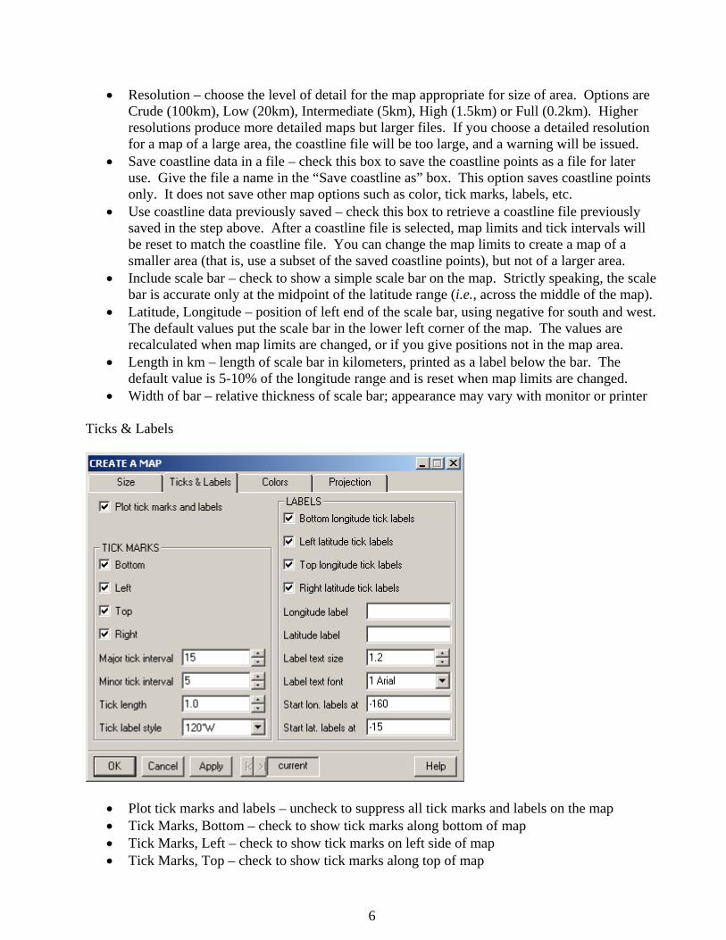
Width of bar – relative thickness of scale bar; appearance may vary with monitor or printer Ticks & Labels

Plot tick marks and labels – uncheck to suppress all tick marks and labels on the map Tick Marks, Bottom – check to show tick marks along bottom of map Tick Marks, Left – check to show tick marks on left side of map Tick Marks, Top – check to show tick marks along top of map

6

Tick Marks, Right – check to show tick marks on right side of map Major tick interval – the number of degrees between major (labeled) tick marks, which are

written at numbers evenly divisible by this interval; default depends on map size. Minor tick interval – the number of degrees between minor (unlabeled) tick marks, starting

with Left Longitude and Bottom Latitude; default depends on map size. There should be an integer number of minor ticks per major tick interval.

Tick length – length of both major and minor tick marks, relative to a standard of 1.0. Minor tick marks are 40% the length of major tick marks.

Tick label style – options for tick mark label style are 120, 120W, 120, or 120W Bottom longitude tick labels – check to show longitude degree labels along bottom of map Left latitude tick labels – check to show latitude degree labels on left side of map Top longitude tick labels – check to show longitude degree labels along top of map Right latitude tick labels – check to show latitude degree labels on right side of map Longitude label – enter text for optional label on bottom axis Latitude label – enter text for optional label on left axis Label text size – relative size of text for tick and axis labels Label text font – font for tick and axis labels. Use Display symbols, colors & fonts from

the CruzPlot menu to display available fonts. Start lon. labels at – left-most longitude on the map at which to start labels on major tick

marks, using negative for west. Default is the first major tick to the east of Left Longitude. Start lat. labels at – bottom-most latitude on the map at which to start labels on major tick

marks, using negative for south. Default is the first major tick north of Bottom Latitude. Colors

7

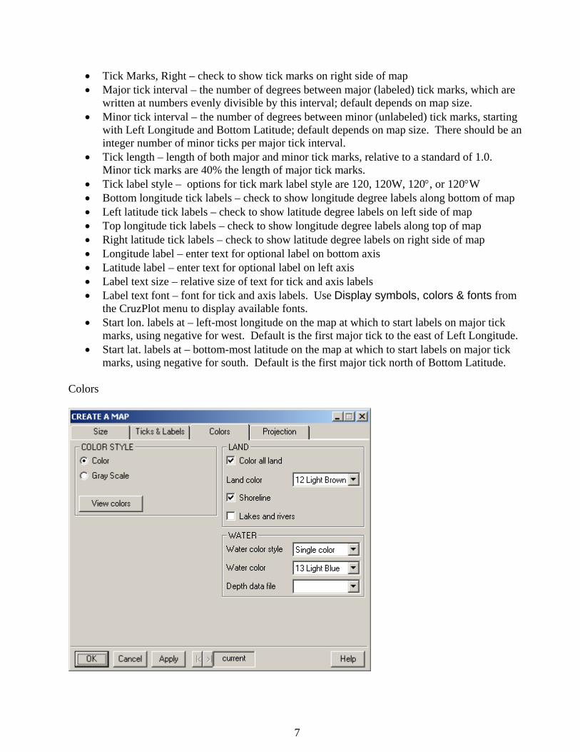
Color Style – select either Color or Gray Scale for the map. The color style choice applies to the map as well as to all symbols, lines and text plotted on it. Use Display symbols, colors & fonts from the CruzPlot menu to display available colors.

Color all land – check this box to fill all land with color; uncheck for no color Land color – select a color for land areas Lakes and rivers – check this box to include lakes and rivers on the map Draw shoreline – check this box to draw a black line at the land-water boundary Water color style – choose “Single color” or “Depth shading” to show depth Water color – if style is “Single color”, select the color for water areas Depth data file – if style is “Depth shading”, select the file containing data for your map.

The depth data file must be created independently with columns lat, lon, depth. Bathymetric data can be obtained at http://www.ngdc.noaa.gov/mgg/gdas/gd_designagrid.html. Specify the area you want and select XYZ format. After download, import the file into S-Plus using File | Import data, and the depth file will appear on the drop-down list in CruzPlot.

Projection

Map projection – choose Cylindrical, Orthographic or Winkel Tripel. The rectangular Cylindrical projection will normally be used. See Fig. 1 for examples and details. At this time, the Orthographic and Winkel projections are still under construction.

Projection factor – specifies amount of north-south stretching relative to east-west in a cylindrical projection, ranging from 0 (plate carre) to 0.8 (Miller) to 1 (Mercator).

Include grid lines – check to show grid lines on the map at major tick intervals Line color – select a color for the grid lines Line width – specify a thickness for the grid lines Line type – select a line type (use Display symbols, colors & fonts to display line types)

8

Plot DAS Data DAS files are text files in a specific format produced by WinCruz, the data entry program used on line-transect cruises at the SWFSC to record searching effort and sightings of mammals and turtles. Sightings

DAS file name – enter the path and name of a DAS file, or use the Browse button to locate

the DAS file. The default is simply an example. Sighting type – choose Mammals, Turtles or Boats. These sighting types are recorded in

different formats in DAS files. Sighting codes – use the drop-down list to select the codes of sightings to be plotted. Each

code is a field-identifiable sighting category. Cetaceans have number codes, while pinnipeds, turtles and boats have letter codes. Click on either of the Sp codes buttons in the VIEW group to display codes sorted by scientific or common name. For multiple selections from the drop-down sighting code list, use control+click or shift+click in the usual way. The order of selection of the sighting codes corresponds to the order of choices for symbols and colors, as well as the order in which they are listed in the legend. Plotting occurs in reverse order to the legend, so if two species occur at the same location, the symbol for the species listed first in the legend will be plotted on top. Sighting codes are actually character strings, not numbers, so if entering sighting codes from the keyboard, use leading zeros – e.g., eastern spinner dolphins are 010, not 10 – and separate multiple entries by commas with no spaces. There is also an option to plot all cetacean sightings in the DAS file. In this case, different sighting codes will be automatically assigned various combinations of symbols and colors, but these may not all be unique.

9

Symbol types – select symbols to be plotted, one symbol for each sighting code, or a single symbol for all species. Each symbol is represented by a number; click on the Symbols, colors button to display the symbols. Use control+click or shift+click for multiple selections. The order of the symbol codes corresponds to the order of the sighting codes. There is also an option to plot sighting codes as symbols – that is, to plot the selected sighting numerical or letter codes instead of symbols at each location. For example, if this option is selected, the character string 013 would be plotted at the position of each striped dolphin sighting instead of a symbol.

Symbol colors – select a color for each symbol, or a single color for all symbols. Each color is represented by a number; click on the Symbols, colors button to display available colors. Use control+click or shift+click for multiple selections. The order of the color codes corresponds to the order of the sighting codes.

Symbol sizes – specify sizes for all symbols relative to standard 1.0, or a single size for all symbols. The order of the size codes corresponds to the order of the sighting codes.

Symbol line widths – widths of lines for all symbols relative to standard 1.0, or a single width for all. The order of the line widths corresponds to the order of the sighting codes.

Preview selection – displays the current selection of sighting codes, colors, symbols, symbol sizes and symbol line widths; close this window before plotting.

Symbols, colors – displays codes for symbols, colors, line types and fonts (same as the Display symbols, colors & fonts display from the CruzPlot menu). Close this window before plotting.

Sp codes, scien – display SWFSC sighting codes sorted by scientific name Sp codes, comm – display SWFSC sighting codes sorted by common name

Filters

10

Sightings to plot – choose one option: all on- and off-effort sightings, either on- or off-effort sightings separately, or no sightings (if plotting effort only). The default definition of effort is standard effort in closing mode, but the effort options can be changed on the Effort page.

Include probable species sightings – if checked, plot will include “probable” identifications Label sightings interactively – if checked, allows interactive identification and labeling of

sightings. After sightings have been plotted, the cursor will change to a cross over the map. A left-click of the mouse near a point will identify the point by cruise number, sighting number and date; a right-click exits interactive mode.

Min, Max Beaufort - only sightings with associated Beaufort sea state values greater than or equal to the minimum and less than or equal to the maximum will be plotted

Month, Day, Year – only sightings recorded on or between the specified dates will be plotted. Month, day, and year are checked independently, so sightings must fit each criterion to be plotted. Example: to plot sightings made each December from 1986 to 2003 specify 1 and 31 for min. and max. day, 12 and 12 for min. and max. month, and 1986 and 2003 for min. and max. year. Effort filters (on Effort tab) are updated to equal sightings filters when sightings filters are changed.

Cruise Number – only sightings with this cruise number will be plotted. Only one cruise number at a time is allowed; leaving the box blank (default) includes all cruise numbers.

Truncation (km) – only sightings less than or equal to this perpendicular distance from the trackline will be plotted. A blank box (default) plots sightings at all distances.

Legend

Legend for sightings – select one option: “No legend” (default) does not plot a legend on the map; “Include legend” plots a legend with symbols and scientific names (corresponding to chosen sighting codes) for species with at least one sighting; “Legend only” plots a legend

11

Legend type – choose whether to make the legend editable or not. An editable legend has more options to control legend appearance, and scientific names will appear in italics. A left click on an editable legend box allows moving and resizing; a right click brings up a window with other legend properties. Individual legend items may also be edited. Symbols and lines in editable legends may appear slightly different than what is plotted on the map. A non-editable legend is useful for a series of maps with a consistent legend format and position. If a non-editable legend is chosen, set legend options below.

Legend Title – enter text to be placed at the top of the legend (optional) Include number of sightings – if checked, after the species name the legend will include the

number of plotted points as “n = ” Box color – choose a white legend box with black border (default), white legend box

without border, or transparent background (legend text is simply placed on top of map) Box width – the right edge of the legend box can be increased or decreased. Text size – the size of legend text can be increased or decreased. Font – font for text in the legend. Default is the font chosen for map labels. Position – specify where to place the legend on the map. Choose a pre-set position at a

corner of the map, or choose ‘Specify exactly’ to specify a position on the map. Latitude, Longitude – position of the upper left corner of the legend when ‘Specify Exactly’

is selected for legend position, using decimal numbers, negative for south and west. Effort

12

Effort to plot – select one option: No effort lines – effort is not plotted Simplified effort – lines are drawn between positions of B (begin) and the last (before

next B) E (end) records in the DAS file. Normally this will produce a single, straight line segment for each day. This simple representation of effort will plot quickly and will generally be an adequate representation for a map of a large area. However, it will not be accurate in some circumstances – for example, if effort for the day included a turn at a waypoint, or if there was an extended off-effort period in the middle of the day.

Detailed effort – lines are drawn between each pair of R (resume) and E (end) records in the DAS file. This representation of effort takes a bit longer, but gives a detailed plot of each segment covered on effort. It assumes straight lines between R and E positions.

Closing/Passing – select to plot effort in closing mode (default), passing mode, or both, and/or sightings during such effort.

Standard/Non-stan. – select to plot standard effort (default), non-standard effort, or both, and/or sightings during such effort. Non-standard effort is regular line-transect effort but, for any of several reasons, is not considered part of the designed survey. Plotting of fine-scale effort is not currently implemented.

Line width – thickness of effort lines relative to standard 1.0 Line color – color of effort lines. Use Display symbols, colors & fonts to display color

choices. Label effort lines interactively – if checked, allows interactive identification and labeling of

on-effort lines. After lines have been plotted, the cursor will change to a cross over the map. A left-click of the mouse near a line will identify the transect by cruise number and date; a right-click exits interactive mode.

Min, Max Beaufort – only effort with associated Beaufort sea states greater than or equal to the minimum and less than or equal to the maximum will be plotted. Selecting effort by Beaufort requires more computation and will take longer to plot.

Month, Day, Year – only effort on or between the specified dates will be plotted. Month, day, and year are checked independently so effort must fit each criterion to be plotted.

Cruise Number – only effort on this cruise will be plotted. Only one cruise number at a time is allowed; leaving the box blank (default) includes all cruise numbers in the DAS file.

Notes: (1) Because mammal, turtle and boat sightings are recorded in different formats in DAS files, only one type may be plotted at a time. However, different sighting types may be plotted sequentially on the same plot. (2) If effort is plotted, the number of R (Resume effort) and E (End effort) records in the DAS file must be equal (they should occur in pairs). If this is not the case, effort is not plotted and a warning is issued. (3) When sightings filters (Beaufort, date and/or cruise number on Filters tab) are changed, effort filters are updated automatically to match them, but not vice-versa. This allows selection of effort to be different from selection of sightings, if desired. (4) Warnings are issued if no sighting codes are selected, if an undefined sighting code is specified from the keyboard, or if no sightings are selected for plotting under the conditions of Beaufort, date, cruise and effort type specified.

13

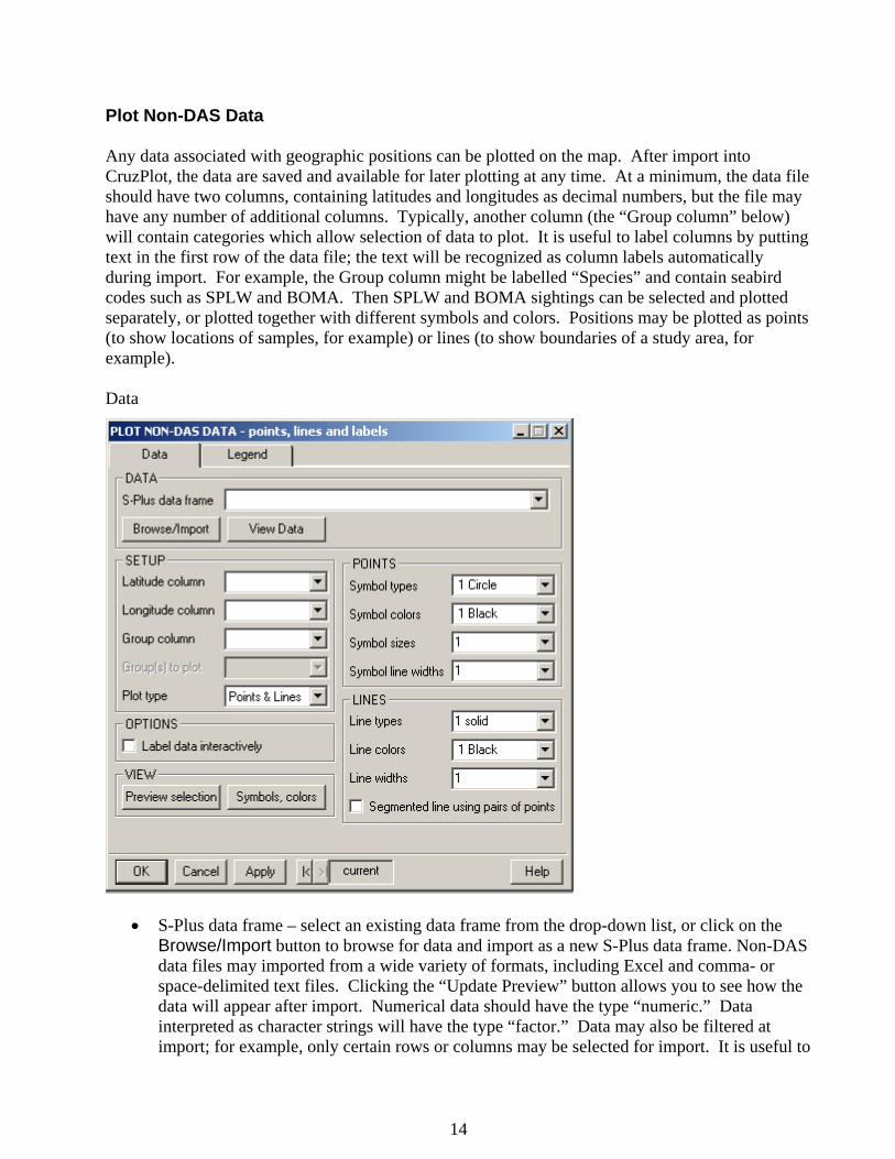
Plot Non-DAS Data Any data associated with geographic positions can be plotted on the map. After import into CruzPlot, the data are saved and available for later plotting at any time. At a minimum, the data file should have two columns, containing latitudes and longitudes as decimal numbers, but the file may have any number of additional columns. Typically, another column (the “Group column” below) will contain categories which allow selection of data to plot. It is useful to label columns by putting text in the first row of the data file; the text will be recognized as column labels automatically during import. For example, the Group column might be labelled “Species” and contain seabird codes such as SPLW and BOMA. Then SPLW and BOMA sightings can be selected and plotted separately, or plotted together with different symbols and colors. Positions may be plotted as points (to show locations of samples, for example) or lines (to show boundaries of a study area, for example). Data

S-Plus data frame – select an existing data frame from the drop-down list, or click on the Browse/Import button to browse for data and import as a new S-Plus data frame. Non-DAS data files may imported from a wide variety of formats, including Excel and comma- or space-delimited text files. Clicking the “Update Preview” button allows you to see how the data will appear after import. Numerical data should have the type “numeric.” Data interpreted as character strings will have the type “factor.” Data may also be filtered at import; for example, only certain rows or columns may be selected for import. It is useful to

14

View Data – displays the selected dataframe; data can be edited from this window. Latitude column – select the column of the dataframe containing latitude values, given as

decimal numbers. If the name of a column begins with the letters “lat”, the name of that column (or the first one, if multiple) will be automatically selected for Latitude column.

Longitude column – select the column of the dataframe containing longitude values, given as decimal numbers. If the name of a column begins with the letters “lon”, the name of that column (or the first one, if multiple) will be automatically selected for Longitude column.

Group column – if you wish to plot a subset of the data, or to plot subsets in different ways (with different symbols, colors or line types, for example), specify the column which contains the identifying labels or values for selection. Leave the box blank to plot all data.

Group(s) to plot – if a Group column has been specified, you may select a single or multiple values from the Group column to plot in any order by using control+click or shift+click. The default (no selection) is to plot all values. The order of selection of multiple groups in this box corresponds to the order of multiple selection of symbols, colors and line types, and the order in which the groups are listed in the legend. Groups are plotted in reverse order, so that if two values occur at the same location, the symbol (or line) for the one that occurs first in the legend will be plotted on top of the second.

Plot type – choose to plot points, lines, both points and lines, or group labels. Selecting Group Labels means to plot the character string itself at the position instead of a symbol – for example, to plot the letter “A” at one set of positions and “B” at another set of positions, where the letters A and B are given in the Group column of the data.

Preview selection – opens a window displaying the current selection of symbols, lines, size, width, colors and groups; close this window before plotting.

Symbols, colors – displays codes for symbols, colors, line types and fonts (same as Display symbols, colors & fonts display from CruzPlot menu). Close this window before plotting.

Symbol types – for points, select one or more symbols to be plotted, including male and female symbols; symbols will be plotted in the order given in Group(s) to plot.

Symbol colors – for points, select one or more color codes for the symbols; colors will be plotted in the order given in Group(s) to plot.

Symbol sizes – for points, select one or more sizes for all symbols relative to standard 1.0; sizes will be plotted in the order given in Group(s) to plot

Symbol line widths – for points, select one or more line thicknesses for all symbols relative to standard 1.0; line widths will be plotted in the order given in Group(s) to plot

Line types – for lines, select one or more line type codes (use Display symbols, colors & fonts to display line types); line types will be plotted in the order given in Group(s) to plot.

Line colors – for lines, select one or more color codes for the lines; colors will be plotted in the order given in Group(s) to plot.

Line widths – for lines, select one or more thickness values for all lines relative to standard 1.0; line widths will be plotted in the order given in Group(s) to plot

Segmented line using pairs of points – check this box to plot lines between alternate sequential positions rather than between each position. For example, use this option if the data file consists of alternating begin and end effort positions.

15

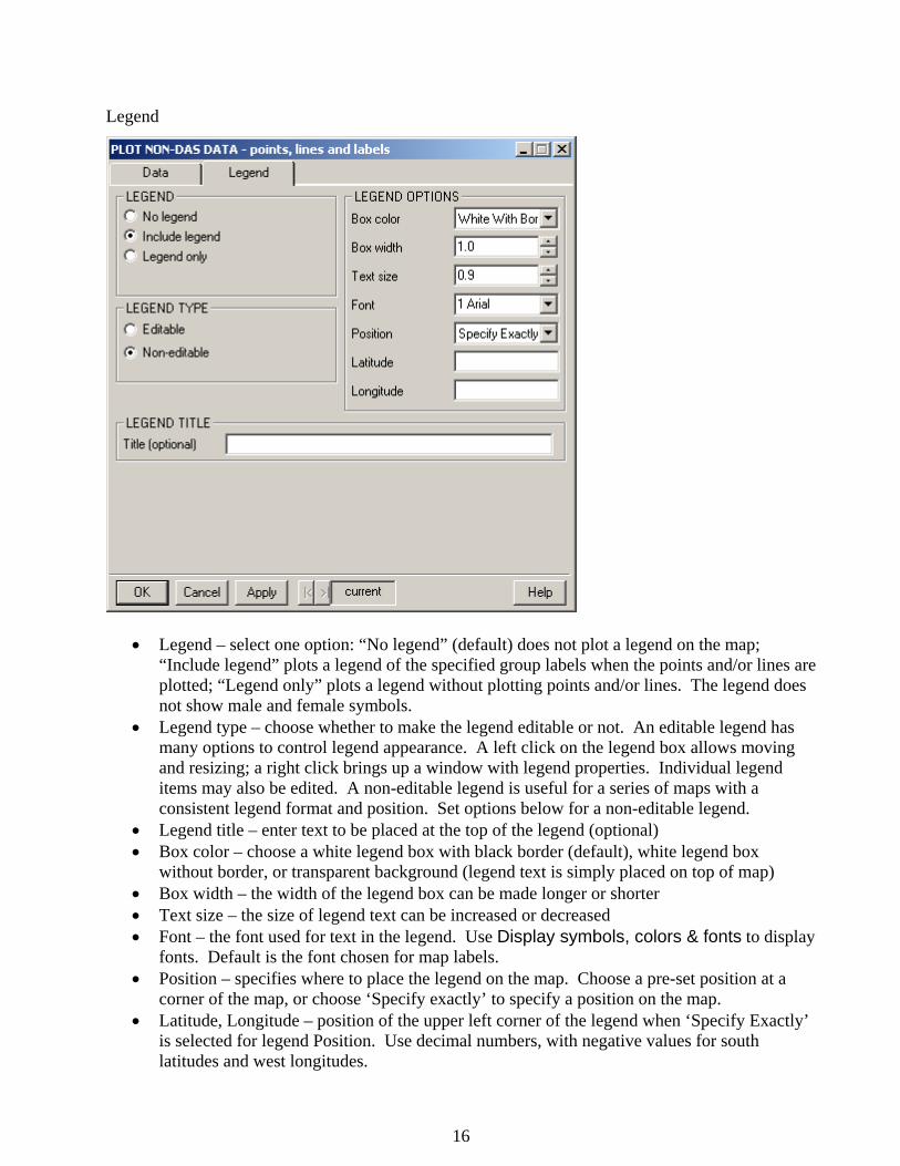
Legend

Legend – select one option: “No legend” (default) does not plot a legend on the map; “Include legend” plots a legend of the specified group labels when the points and/or lines are plotted; “Legend only” plots a legend without plotting points and/or lines. The legend does not show male and female symbols.

Legend type – choose whether to make the legend editable or not. An editable legend has many options to control legend appearance. A left click on the legend box allows moving and resizing; a right click brings up a window with legend properties. Individual legend items may also be edited. A non-editable legend is useful for a series of maps with a consistent legend format and position. Set options below for a non-editable legend.

Legend title – enter text to be placed at the top of the legend (optional) Box color – choose a white legend box with black border (default), white legend box

without border, or transparent background (legend text is simply placed on top of map) Box width – the width of the legend box can be made longer or shorter Text size – the size of legend text can be increased or decreased Font – the font used for text in the legend. Use Display symbols, colors & fonts to display

fonts. Default is the font chosen for map labels. Position – specifies where to place the legend on the map. Choose a pre-set position at a

corner of the map, or choose ‘Specify exactly’ to specify a position on the map. Latitude, Longitude – position of the upper left corner of the legend when ‘Specify Exactly’

is selected for legend Position. Use decimal numbers, with negative values for south latitudes and west longitudes.

16

** Troubleshooting notes: If data from an imported file do not plot on the map, check that: (1) data might have been plotted on another map if more than one map is open; (2) latitude and longitude are represented as decimal numbers, with negative values for west longitudes and south latitudes; (3) columns containing latitude and longitude values have been correctly specified in the Latitude and Longitude boxes in the dialog window; and (4) latitude and longitude columns have the correct data type of “double.” To check data type, click the View Data button and select (highlight) the latitude or longitude column. Right-click and choose Change Data Type to check the current data type and change it to “double” if necessary. Add Title to Map

Title – the title will appear on one line centered above the map. Note that a title created with Add Title to Map cannot be edited; use Add Text to Map to create an editable title.

Text size – character size of text can be increased or decreased Text color – color of text can be set with a color code Font – font of text in title. Default is the font chosen for map labels. Colors, fonts – displays options for text color and font

Add Text to Map Clicking this menu item allows editable text to be placed on a map. No dialog window appears. Left-click allows moving and resizing of the text; right-click brings up a window with properties.

17

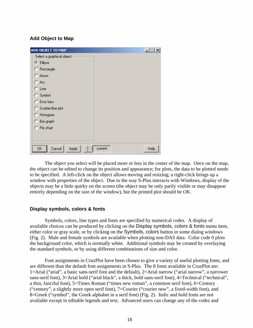
Add Object to Map

The object you select will be placed more or less in the center of the map. Once on the map, the object can be edited to change its position and appearance; for plots, the data to be plotted needs to be specified. A left-click on the object allows moving and resizing; a right-click brings up a window with properties of the object. Due to the way S-Plus interacts with Windows, display of the objects may be a little quirky on the screen (the object may be only partly visible or may disappear entirely depending on the size of the window), but the printed plot should be OK. Display symbols, colors & fonts Symbols, colors, line types and fonts are specified by numerical codes. A display of available choices can be produced by clicking on the Display symbols, colors & fonts menu item, either color or gray scale, or by clicking on the Symbols, colors button in some dialog windows (Fig. 2). Male and female symbols are available when plotting non-DAS data. Color code 0 plots the background color, which is normally white. Additional symbols may be created by overlaying the standard symbols, or by using different combinations of size and color. Font assignments in CruzPlot have been chosen to give a variety of useful plotting fonts, and are different than the default font assignments in S-Plus. The 8 fonts available in CruzPlot are: 1=Arial (“arial”, a basic sans-serif font and the default), 2=Arial narrow (“arial narrow”, a narrower sans-serif font), 3=Arial bold (“arial black”, a thick, bold sans-serif font), 4=Technical (“technical”, a thin, fanciful font), 5=Times Roman (“times new roman”, a common serif font), 6=Century (“century”, a slightly more open serif font), 7=Courier (“courier new”, a fixed-width font), and 8=Greek (“symbol”, the Greek alphabet in a serif font) (Fig. 2). Italic and bold fonts are not available except in editable legends and text. Advanced users can change any of the codes and

18

utilize additional colors and fonts. However, unless changes to codes are explicitly changed back to the defaults, changes will remain in effect for other users of the shared drive, so this is not recommended. Also, codes will be reset to CruzPlot defaults whenever an update occurs. If you want to customize fonts, colors or symbols, run CruzPlot on your own computer and make customized changes locally. The exact appearance of symbols, colors, line types and fonts will vary by monitor and printer. Print the Display symbols, colors & fonts page to see exactly how they will look for your hardware. A larger range of gray scales can be produced by creating a color map but printing it in black-and-white. If the Display symbols, colors & fonts display has been produced after a map and is still open, CruzPlot will attempt to plot points and lines on the Display symbols page rather than on the map. Either close the Display symbols page before plotting, or create the Display symbols page before creating the map. Open CruzPlot Manual Clicking this menu item will open a window displaying this manual.

19

30E 60E 90E 120E 150E 180 150W 120W 90W 60W 30W 0

30E 60E 90E 120E 150E 180 150W 120W 90W 60W 30W 0

60S

30S

0

30N

60N

60S

30S

0

30N

60N

Projection factor = 0

30E 60E 90E 120E 150E 180 150W 120W 90W 60W 30W 0

30E 60E 90E 120E 150E 180 150W 120W 90W 60W 30W 0

60S

30S

0

30N

60N

60S

30S

0

30N

60N

Projection factor = 0.8

30E 60E 90E 120E 150E 180 150W 120W 90W 60W 30W 0

30E 60E 90E 120E 150E 180 150W 120W 90W 60W 30W 0

60S

30S

0

30N

60N

60S

30S

0

30N

60N

Projection factor = 1.0

30E 60E 90E 120E 150E 180 150W 120W 90W 60W 30W 0

30E 60E 90E 120E 150E 180 150W 120W 90W 60W 30W 0

60S

30S

0

30N

60N

60S

30S

0

30N

60N

Projection factor = 0

30E 60E 90E 120E 150E 180 150W 120W 90W 60W 30W 0

30E 60E 90E 120E 150E 180 150W 120W 90W 60W 30W 0

60S

30S

0

30N

60N

60S

30S

0

30N

60N

Projection factor = 0.8

30E 60E 90E 120E 150E 180 150W 120W 90W 60W 30W 0

30E 60E 90E 120E 150E 180 150W 120W 90W 60W 30W 0

60S

30S

0

30N

60N

60S

30S

0

30N

60N

Projection factor = 1.0

Fig. 1. Cylindrical map projections in CruzPlot. Cylindrical projections include a range of projections controlled by a factor that determines the amount of north-south stretching relative to east-west stretching. A map created with a factor of 0 is an equirectangular projection, also known as a plate carrée (“flat and square”) projection when centered on the equator. It has an equal north-south scale everywhere on the map. For small- to moderate-sized areas, this will give a map that looks good and is easy to read, and it is the default projection in CruzPlot. To minimize distortion, the default projection in CruzPlot has the standard parallel, where the scale is true, in the middle of the latitude range (that is, from left to right across the middle of the map). A cylindrical projection with a factor of 1 is the Mercator projection, which has north-south stretching equal to east-west stretching; areas are progressively distorted at high latitudes. A map with a factor of 0.8 has less distortion at high latitudes and is known as a Miller projection.

20

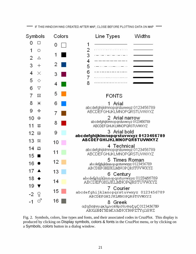
Fig. 2. Symbols, colors, line types and fonts, and their associated codes in CruzPlot. This display is produced by clicking on Display symbols, colors & fonts in the CruzPlot menu, or by clicking on a Symbols, colors button in a dialog window.

21