crow amsaa

Crow/AMSAA Reliability Growth Plots And there use in Interpreting Meridian Energy Ltd’s, Main Unit Failure Data

by

Nigel Comerford

Areva T&D New Zealand

Purpose

To explore the Crow/AMSAA model and its use in monitoring and projecting reliability growth or performance of existing plant and apply this technique to the main unit failures

of Meridian Energy’s generating system, allowing confirmation of reliability improvement, those improvements to be quantified, correlation of operational events

against reliability, and forecast of failure rates.

16th Annual Conference 2005- Rotorua

of 22


This paper is the property of VANZ. Reproduction is not permitted without permission.

of 22

1.0 Executive Summary Meridian Energy is a New Zealand state owned enterprise, which operates, among other assets, 38 hydro machines in a deregulated electricity market. It is the Forced Outages or unit failures as they apply to this system that is the subject of this paper.

The key objectives are to explore the Crow/AMSAA model and its use in monitoring and projecting reliability growth or performance of existing plant and apply this technique to the main unit failures of Meridian Energy’s generating system, allowing confirmation of reliability improvement, those improvements to be quantified, correlation of operational events against reliability, and forecast of failure rates.

Although Forced Outages, within this industry, do not have a great affect on availability they do cost money and expose the business to risk.

The Crow/AMSAA technique involves plotting, most commonly, cumulative failures Vs cumulative time on a log-log scale with the resulting straight lines’ slope indicating improving, deteriorating, or constant reliability. Instantaneous failure rate can be determined, and due to the straight-line nature of the plots, forecasts can be made of failures into the future. This method handles mixed failure modes, so is therefore suitable for the complex nature of the generating units, which at a system level exhibit random failures of mixed modes.

A review of the last five years of Forced Outage data has determined the average estimated cost of a Forced Outage at $6500 per event.

Crow/AMSAA plots of the last nine years of data show that although on average the reliability of the system is constant there was a deteriorating situation up until the turn of the century, then there has been consistent year on year improvements; that is we were at a level then deteriorated and have since improved to be at our best now.

This performance mapped against operational history shows this improving situation started after the unsettled period of the late 90’s and the Automation & Remote Control project finishing and seems to have been driven by the Event Analysis system. The analysis also shows that although the numbers of machine starts and the amount of generation have both increased slightly and that the direct maintenance spend has dropped there has still been a great improvement in reliability.

A sound management tool has been proven which allows forecasting of Forced Outages allowing their affect on availability and unplanned maintenance costs to be known.

Combining this information with the cost of each Forced Outage, shows that if there had been no improvement of the performance from the 1999 – 2000 period we could have expected to see as much as 150 extra Forced outages in the last year alone, the reduction in Forced Outages that has been achieved equates to savings of $975,000 / year.



of 22

2.0 Contents 1.0 Executive Summary ............................................................................................. 2 2.0 Contents ..................................................................................................................... 3 3.0 Introduction................................................................................................................ 4

3.1 Objectives .............................................................................................................. 4 3.2 Meridian Energy’s Generation System.................................................................. 4 3.3 Why should we reduce Forced Outages & how will measuring Forced Outage Rate in this manner help .............................................................................................. 4

4.0 The Duane Crow/AMSAA Model ............................................................................. 5 4.1 History.................................................................................................................... 5 4.2 Application............................................................................................................. 5 4.3 Crow/AMSAA Model Theory ............................................................................... 7 4.3.1 Further Developments......................................................................................... 9

5.0 Crow/AMSAA Software............................................................................................ 9 6.0 Failure Data & Definitions....................................................................................... 10

6.1 Definition of a Failure.......................................................................................... 10 6.2 Period of Analysis................................................................................................ 10 6.3 Data Sets .............................................................................................................. 10

7.0 The Cost of a Failure................................................................................................ 11 7.1 Why is it important to know what Forced Outages cost...................................... 11 7.2 Forced Outage cost build-up................................................................................ 11

8.0 Meridian Energy’s FO data as Crow/AMSAA plots ............................................... 12 8.1 Complete Nine-Year Plot..................................................................................... 12 8.2 First Four-Years Plot............................................................................................ 13 8.3 Last 5-Year Plot ................................................................................................... 13 8.4 Year by Year Plot................................................................................................. 14 8.5 2003 – 2004 Financial Year plot.......................................................................... 15

9.0 Organisation Operational History & Correlation with Failure Rate........................ 15 1.1.1 9.1 Operational & Maintenance Systems Timeline ................................... 16 1.1.2 9.2 Operational Parameters & Beta Value Comparison ............................ 17 9.3 Correlation Between Failure Rate and Historic Parameters ................................ 18

10.0 Failure Forecasting................................................................................................. 19 10.1 Limitations ......................................................................................................... 19 10.2 Why do we want to Forecast?............................................................................ 19 10.3 Forecasting Method ........................................................................................... 19

11.0 Conclusions............................................................................................................ 20 Acknowledgements........................................................................................................ 22 References...................................................................................................................... 22



of 22

3.0 Introduction

3.1 Objectives The key objective of this paper is to explore the Crow/AMSAA technique and to apply it to the evaluation of historic and future ‘Forced Outage’ occurrences of Meridian Energy’s generating plant. This will include an overview of the history and theory of the Crow/AMSAA Reliability Growth Model to enable a depth of understanding as to apply the technique; choose software to allow cost effective application, extract and format Forced Outage data from Meridian Energy’s databases which will produce suitable inputs for the model, determine an average estimated cost of a Forced Outage to enable the quantification in dollars terms of improvements, create Crow/AMSAA plots to interpret, & confirm historic reliability growth and or degradation, and to build a high level time-line of Meridian Energy’s operational and maintenance history, to allow correlation of reliability against historic events, with an aim of learning what factors are propagating growth. Additionally forecasting of failure rate, allowing more certainty around availability and financial budgets, the quantification of proposed reliability improvement plans, and the uses for management of Crow/AMSAA plots will all be discussed.

3.2 Meridian Energy’s Generation System Meridian Energy is the largest producer of hydro electricity in New Zealand. It operates nine large hydro stations, comprising 38 main generating machines, spread across the lower South Is of New Zealand with a combined installed capacity of 3500MW. It is this system or fleet of 38 hydro machines, viewed as a whole, which is the subject of this paper in respect to applying the Crow/AMSAA technique. This system of machines, which vary from multi unit, 120MW Francis turbine stations, to a 25MW, single unit station, Kaplan machine, are all controlled remotely from one location and unmanned. The system operates within a deregulated electricity market where generation is sold based on availability of both machines and fuel Vs demand.

3.3 Why should we reduce Forced Outages & how will measuring Forced Outage Rate in this manner help Forced outages do not have a great impact on availability however they do impact the systems exposure to risk, cost money, and they indicate generally the overall health of the system.

The fewer Forced Outages there are the less exposure to ‘Revenue Opportunity Cost’, the cost of lost generation due to the units sudden unavailability and the systems inability to pick-up the generation, and the cost of market imposed penalties for repeated failure to deliver offered generation.

Overall the health of the generating system is perceived to be better when fewer Forced Outages are occurring. It is seen as an indicator of the general health of the plant, the fewer Forced Outages there are, the fewer high priority alarms, the fewer corrective maintenance work orders, and the fewer unknown plant conditions. Our probable exposure to “the big one”, that 1 in 200 Forced Outage event that causes considerable plant damage, cost, or injury is less frequent when our failure rate is less.

Effective measuring, allowing transparency of reliability, cusps in the failure rate, and Forced Outage forecasting and quantification will allow better management decisions to



of 22

be made on factors affecting Forced Outages. This will also allow decisions to be made on the cost of maintaining a set Forced Outage Rate or wanting to improve it further.

4.0 The Duane Crow/AMSAA Model Reliability Growth Plots have a variety of names, such as Duane Plots, Crow Plots, or Crow/AMSAA Plots. The technique involves plotting, most commonly, cumulative failures Vs cumulative time on a log-log scale with the resulting straight lines’ slope indicating improving, deteriorating, or constant reliability. The literal beta value of >1 shows failures increasing, 1 indicates constant failures, and <1 shows failure rate improving. Instantaneous failure rate can be determined, and due to the straight-line nature of the plots, forecasts can be made of failures into the future. This method handles mixed failure modes, so is therefore suitable for the complex nature of the generating units, which at a system level exhibit random failures of mixed modes.

4.1 History Reliability Growth Modeling has its origins in the tracking of the improvements in manufacturing times and has been exhaustedly demonstrated as a true log-log phenomenon. T. P. Wright in 1936 pioneered an idea that improvements in the time to manufacture an airplane could be described mathematically. Wrights findings showed that, as the quantity of airplanes were produced in sequence, the direct labour input per plane decreased in a mathematical pattern that forms a straight line when plotted on log-log paper.4

Learning curves were used extensively by General Electric and a GE reliability engineer made log-log plots of cumulative MTBF Vs cumulative time, which gave a straight line, (Duane 1964). James Duane developed a deterministic postulate for monitoring failure rates of more complex systems over time using a log-log plot with straight lines.

At the US Army Material Systems Analysis Activity (AMSAA) during the mid 1970’s Larry Crow converted Duane’s postulate into mathematical and statistical proof via Weibull statistics in MIL-HDBK-1893.

By the end of the seventies there were several dozen different growth models in use. The Aerospace Industries Association Technical Management Committee studied this array of methods as applied to mechanical components and concluded the Crow/AMSAA model was the best. The U.S. Air Force study, conducted by Dr Abernethy1, including both mechanical and electrical controls, reached the same conclusion.

4.2 Application Although the Crow/AMSAA model has its base in measuring reliability growth, defined as, “The positive improvement in a reliability parameter over a period of time due to changes in product design or the manufacturing process”, it is the wider definition of reliability growth management, which is defined as, “The systematic planning for reliability achievement as a function of time and other resources, and controlling the ongoing rate of achievement by reallocating of resources based on comparison between planned and assessed reliability values”, which is more relevant for our purposes.

With reliability growth management in mind the Crow/AMSAA plot has more recently found other important applications. Many industries are routinely doing Crow/AMSAA analysis and it is considered best practice for tracking fleets of units to trend reliability,



of 22

safety, and maintainability events of interest. It is capable of utilizing dirty data, including missing data sets, and mixtures of failure modes. It is also applicable for tracking parameters that interest management and forecasting their future levels.

The Crow/AMSAA model will be applied to the Forced Outage data of Meridian’s systems of generators. Cumulative failures over cumulative time are plotted using suitable software, (see below). This delivers a graphical straight-line plot, with a goodness of fit test, and extrapolation. Failure rate, hazard rate, and the slope of the line are all delivered which will allow realisation of the following benefits.

Trend charts that make reliability growth or degradation more visible and manageable.

The progress of the reliability improvement program, the effects of changes and improvements are measured and displayed.

Reliability predictions are available early to compare against business requirements.

Adverse system reliability trends are indicated much sooner and more accurately than rolling averages.

System or component level reliability trends can be measured even with mixed failure modes.

It is important to note that the reliability improvement process is modeled, not just the physical system. For example a system may have a number of components that initially exhibit wear-in characteristics, which as this phase elapses, a generally improving failure rate is exhibited in the CA model. However the CA model will show equally well the instigation of a Condition Monitoring program or the doubling of RCFA effort.



of 22

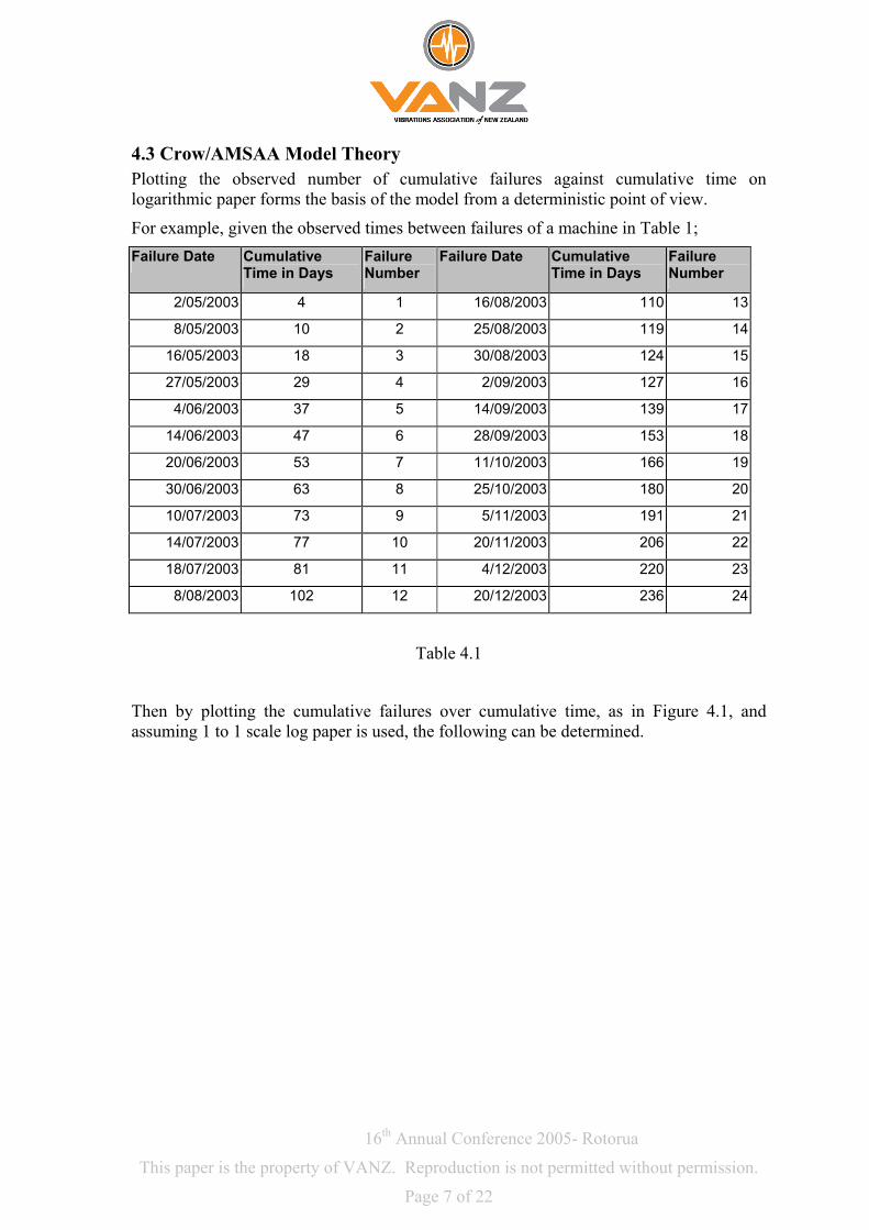
4.3 Crow/AMSAA Model Theory Plotting the observed number of cumulative failures against cumulative time on logarithmic paper forms the basis of the model from a deterministic point of view.

For example, given the observed times between failures of a machine in Table 1; Failure Date Cumulative

Time in Days Failure Number

Failure Date Cumulative Time in Days

Failure Number

2/05/2003 4 1 16/08/2003 110 13

8/05/2003 10 2 25/08/2003 119 14

16/05/2003 18 3 30/08/2003 124 15

27/05/2003 29 4 2/09/2003 127 16

4/06/2003 37 5 14/09/2003 139 17

14/06/2003 47 6 28/09/2003 153 18

20/06/2003 53 7 11/10/2003 166 19

30/06/2003 63 8 25/10/2003 180 20

10/07/2003 73 9 5/11/2003 191 21

14/07/2003 77 10 20/11/2003 206 22

18/07/2003 81 11 4/12/2003 220 23

8/08/2003 102 12 20/12/2003 236 24

Table 4.1

Then by plotting the cumulative failures over cumulative time, as in Figure 4.1, and assuming 1 to 1 scale log paper is used, the following can be determined.



of 22

Log-Log Plot of Machine Failures

0.1

1

10

100

1000

1 10 100 1000

Cumulative Time Days

Cum

ulat

ive

Failu

res

FailureNumber

8.1cm

10cmLambda 0.29

Beta 0.81

Figure 4.1

Cumulative Failure Events at time t is represented by n(t). The scale parameter λ, is the intercept on the y-axis of n(t) at t = 1 unit. With the data plotted in Figure 1, λ is read off as 0.29. The slope β can be measured graphically providing log paper with a 1 x 1 scale is used; in the above case Beta is 8.1 / 10 = 0.81.

The model’s intensity function p(t) measures the instantaneous failure rate at each cumulative time point. The intensity function is;

1)( −= βλβρ tt

The log of the cumulative failure events n(t) verse the log of cumulative time is a liner plot if the model applies;

βλttn =)(

Taking natural logarithms of the equation yields; LntLntLnn βλ +=)(

Which implies the equation above is a straight line on logarithmic paper.



of 22

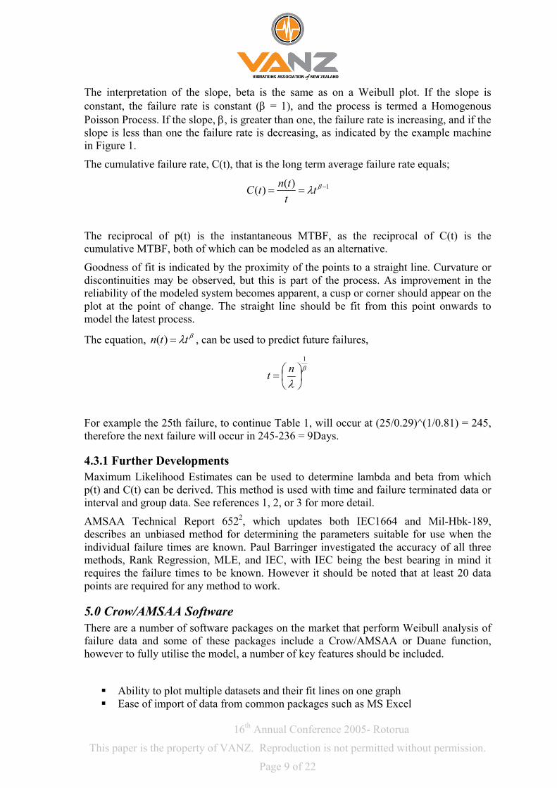
The interpretation of the slope, beta is the same as on a Weibull plot. If the slope is constant, the failure rate is constant (β = 1), and the process is termed a Homogenous Poisson Process. If the slope, β, is greater than one, the failure rate is increasing, and if the slope is less than one the failure rate is decreasing, as indicated by the example machine in Figure 1.

The cumulative failure rate, C(t), that is the long term average failure rate equals;

1)()( −== βλtttntC

The reciprocal of p(t) is the instantaneous MTBF, as the reciprocal of C(t) is the cumulative MTBF, both of which can be modeled as an alternative.

Goodness of fit is indicated by the proximity of the points to a straight line. Curvature or discontinuities may be observed, but this is part of the process. As improvement in the reliability of the modeled system becomes apparent, a cusp or corner should appear on the plot at the point of change. The straight line should be fit from this point onwards to model the latest process.

The equation, , can be used to predict future failures, βλttn =)(

β

λ

1

⎟⎠⎞

⎜⎝⎛=

nt

For example the 25th failure, to continue Table 1, will occur at (25/0.29)^(1/0.81) = 245, therefore the next failure will occur in 245-236 = 9Days.

4.3.1 Further Developments Maximum Likelihood Estimates can be used to determine lambda and beta from which p(t) and C(t) can be derived. This method is used with time and failure terminated data or interval and group data. See references 1, 2, or 3 for more detail.

AMSAA Technical Report 6522, which updates both IEC1664 and Mil-Hbk-189, describes an unbiased method for determining the parameters suitable for use when the individual failure times are known. Paul Barringer investigated the accuracy of all three methods, Rank Regression, MLE, and IEC, with IEC being the best bearing in mind it requires the failure times to be known. However it should be noted that at least 20 data points are required for any method to work.

5.0 Crow/AMSAA Software There are a number of software packages on the market that perform Weibull analysis of failure data and some of these packages include a Crow/AMSAA or Duane function, however to fully utilise the model, a number of key features should be included.

Ability to plot multiple datasets and their fit lines on one graph Ease of import of data from common packages such as MS Excel



of 22

Fully scalable, colour, and editable graphs, which can be exported easily to common software.

Ease of extrapolation of both the x and the y axis Able to calculate both cumulative and instantaneous failure rates. Provide a choice of methods, i.e. Rank Regression, IEC, and MLE Able to convert data from interval to cumulative Ability to plot in either discrete failures of MTBF.

A number of software packages were trailed for this project, however ‘WinSMITH Visual’ was chosen as it fulfilled all the above criteria.

6.0 Failure Data & Definitions

6.1 Definition of a Failure Failures as discussed in the project are made up of four types;

The ‘Tripping’ of a main generating unit, that is, a unit unexpectedly shutting down while still connected to the grid

A unit being forced from service due to imminent failure, that is, a unit with a known recently developed fault that is purposefully shut down, before it ‘Trips’, to repair that fault

A unit failing to start when called upon, that is, the unit being given a start command and the unit failing to be online within a prescribed time

And a unit failing to stop, that is, after a stop command is given, the unit failing to come to a complete stop within a prescribed time.

All of these types of failures are classified by ‘North American Electricity Reliability Council’ codes, such as U1, U2, U3, SF, and all of these failures can occur from a mixture of failure mechanisms and modes, in addition to the expected electrical & mechanical failure modes, causes such as PLC code, operational policy, human error, and faults on the connected transmission grid operator’s system, causing unit failures, are all included.

6.2 Period of Analysis Failure data, as defined above, is available in electronic form for Meridian Energy’s generating system dating back approximately 15Years, however due to the diminishing relevance of past data and the difficulty in matching operational history, it will be the last 9 years data that will be included in the analysis with an increasing focus on the more recent data. The period covered will be from the end of July 1995 to the end of June 2004.

6.3 Data Sets Initially the nine-year total, nine year, (year by year), first four years, last five years, and last 12 months data sets will be analysed, with particular attention being paid to cusps and discontinuities. Further more detailed plots will also be made where appropriate to investigate cusps and trends.



of 22

7.0 The Cost of a Failure

7.1 Why is it important to know what Forced Outages cost If the cost of forced outages is known, this can be used by management, in making decisions on the affect Forced Outages have on business and the cost of any effort in maintaining or reducing the Forced Outage Rate Vs any financial benefit by that reduction to the business.

7.2 Forced Outage cost build-up An estimate of the average cost of a Forced Outage has been determined based on the last five years of Forced Outage data. It comprises of direct costs including the actual costs to repair failures and the indirect costs such as the cost of RCFA and ROC.

Direct Costs

Average cost of the Initial Callout Work Order, based $330 on the past 12 months of callouts.

Average cost of the Follow-up Work Orders to actually $815 repair the fault, based on the past 12 months of Forced

Outages.

Average cost per Forced Outage over the last five years $440 of the big failure events. Of which there has been three,

MAN03 Baffle Plate, AVI Battery Bank, and BEN03 CB.

Indirect Costs

Average cost of Asset Coordinators, Tactical Engineers, $1000 and AREVA Engineers time for RCFA per Failure Event

based on a subjective estimate @$100/Hr

Average cost of ROC per Forced Outage based on data $3430 from the last five years.

Total $6015

This estimate is sensitive to the accuracy of the data within our CMMS and is drawn for a number of systems, as there is no consistent effort to record the true actual cost of each Forced Outage. It is also of note that the affect of ROC seems much less in recent years than say four or five years ago. This cost could be further inflated by less tangible costs such as the cost of disruption to scheduled work due to a Forced Outage or the increased personal risk associated with responding to a callout after-hours.



of 22

So, based on a review of the last five years of Forced Outage data, on average, each forced outage is estimated to cost, allowing for the time cost of money, and other factors mentioned above, approximately $6500.

8.0 Meridian Energy’s FO data as Crow/AMSAA plots

8.1 Complete Nine-Year Plot

Figure 8.1

The failure data from the last nine financial years, from July 1995 to the end of June 2004, has been plotted above in Figure 8.1, using the IEC method. The plot shows a beta value of 0.969, which indicates that over this period, on average, reliability has been relatively constant, i.e. no improvement or degradation. However when the discrete points are examined cusps can be seen indicating periods where improvements have been made and periods when degradation in failure rate are evident.

The Cumulative Failure Rate is 0.01874 and the Instantaneous Failure Rate is 0.01751, these two figures are very close, again indicating little overall improvement, on average, in the last nine years.

Extrapolation of the plot shows that if failures were to continue at the above instantaneous rate there would be 153 failures in the upcoming financial year.



of 22

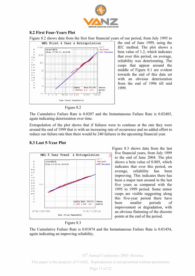
8.2 First Four-Years Plot Figure 8.2 shows data from the first four financial years of our period, from July 1995 to

the end of June 1999, using the IEC method. The plot shows a beta value of 1.2, which indicates that over this period, on average, reliability was deteriorating. The cusps that appear around the middle of Figure 8.1 are evident towards the end of this data set with an obvious deterioration from the end of 1996 till mid 1999.

Figure 8.2

The Cumulative Failure Rate is 0.0207 and the Instantaneous Failure Rate is 0.02485, again indicating deterioration over time.

Extrapolation of the plot shows that if failures were to continue at the rate they were around the end of 1999 that is with an increasing rate of occurrence and no added effort to reduce our failure rate then there would be 240 failures in the upcoming financial year.

8.3 Last 5-Year Plot Figure 8.3 shows data from the last

five financial years, from July 1999 to the end of June 2004. The plot shows a beta value of 0.805, which indicates that over this period, on average, reliability has been improving. This indicates there has been a major turn around in the last five years as compared with the 1995 to 1999 period. Some minor cusps are visible suggesting along this five-year period there have been smaller periods of improvement or degradation, with an obvious flattening of the discrete points at the end of the period.

Figure 8.3

The Cumulative Failure Rate is 0.01874 and the Instantaneous Failure Rate is 0.01454, again indicating an improving reliability.



of 22

Extrapolation of the plot shows that if failures were to continue at the above rate there would be 126 failures in the upcoming financial year. This is less than both the 9-year and first 4-year plots.

Looking at these two fit lines on the same graph, Figure 8.4, shows this obvious improvement graphically by the contrast in slope of the two fit lines.

Figure 8.4 8.4 Year by Year Plot Figure 8.5 shows the period on a year-by-year basis with a fit line for each year indicating the beta value. The changing rate of occurrence of Forced Outages can clearly be seen both graphically and by the changing beta value, 1995 and 1996 show a period of improving reliability on par with 2000, to 2002, however the financial years 1997 to 1999 show a period of decreasing reliability with 1997 showing the worst performance. The most recent year shown, FY2003-2004, the financial year just past, shows a strong improvement compared with the previous three years.

Figure 8.5



of 22

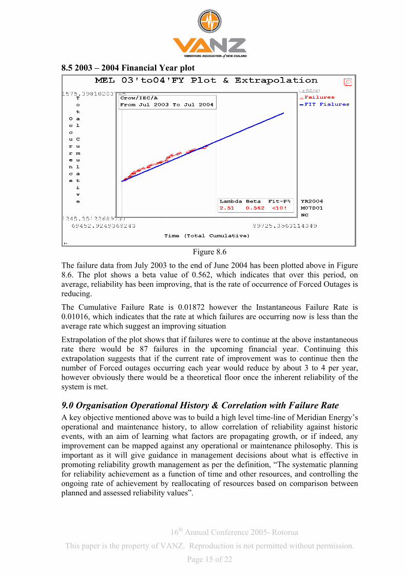
8.5 2003 – 2004 Financial Year plot

d of June 2004 has been plotted above in Figure 8.6. The plot shows a beta value of h indicates that over this period, on

hich indicates that the rate at which failures are occurring now is less than the

ing financial year. Continuing this

tion Operational History & Correlation with Failure Rate A key objective mentioned above was to build a high level time-line of Meridian Energy’s

toric operational and maintenance history, to allow correlation of reliability against his

Figure 8.6

The failure data from July 2003 to the en0.562, whic

average, reliability has been improving, that is the rate of occurrence of Forced Outages is reducing.

The Cumulative Failure Rate is 0.01872 however the Instantaneous Failure Rate is 0.01016, waverage rate which suggest an improving situation

Extrapolation of the plot shows that if failures were to continue at the above instantaneous rate there would be 87 failures in the upcomextrapolation suggests that if the current rate of improvement was to continue then the number of Forced outages occurring each year would reduce by about 3 to 4 per year, however obviously there would be a theoretical floor once the inherent reliability of the system is met.

9.0 Organisa

events, with an aim of learning what factors are propagating growth, or if indeed, any improvement can be mapped against any operational or maintenance philosophy. This is important as it will give guidance in management decisions about what is effective in promoting reliability growth management as per the definition, “The systematic planning for reliability achievement as a function of time and other resources, and controlling the ongoing rate of achievement by reallocating of resources based on comparison between planned and assessed reliability values”.

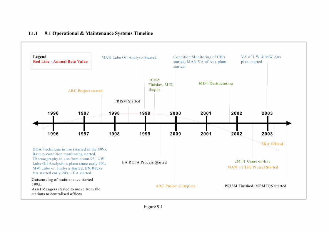
1.1.1 9.1 Operational & Maintenance Systems Timeline

1996 1997 1998 1999 2000 2001 2002 2003

DGA Technique in use (started in the 80's), Battery condition monitoring started, Thermography in use from about 93', UW Lube Oil Analysis in place since early 90's, MW Lube oil analysis started, BN Racks VA started early 90's, PDA started.

1996 1997 1998 1999 2000 2001 2002 2003

ARC Project started

MAN Lube Oil Analysis Started

EA RCFA Process Started

ARC Project Complete

Condition Monitoring of CB's started, MAN VA of Aux plant started

2MTT Came on-lineMAN 1/2 Life Project Started

VA of UW & MW Aux plant started

TKA O/Haul

ECNZ Finishes, MEL Begins

MDT Restructuring

PRISM Started

Outsourcing of maintenance started 1995,Asset Mangers started to move from the stations to centralised offices

PRISM Finished, MEMFOS Started

LegendRed Line - Annual Beta Value

Figure 9.1

c25992 18412203 13/12/2006

GEG7144 Reliability Applications Unit Advisor Emile Eerens

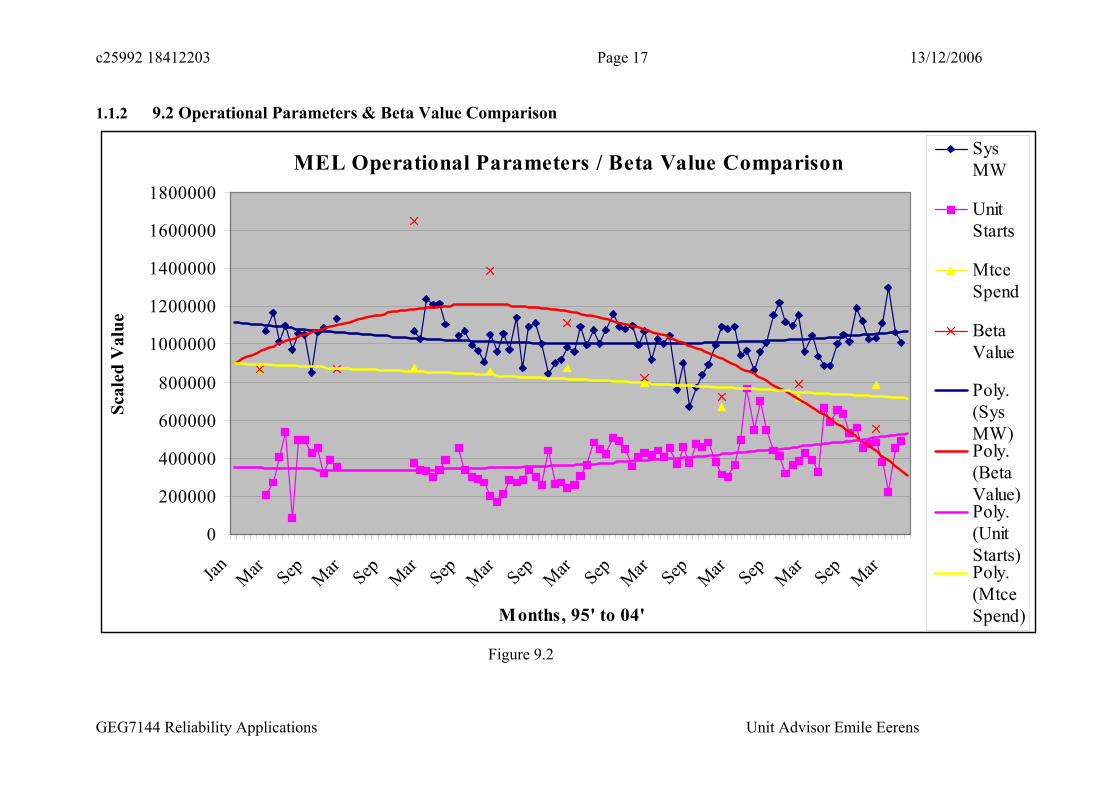
1.1.2 9.2 Operational Parameters & Beta Value Comparison

MEL Operational Parameters / Beta Value Comparison

0

200000

400000

600000

800000

1000000

1200000

1400000

1600000

1800000

Jan Mar Sep Mar Sep Mar Sep Mar Sep Mar Sep Mar Sep Mar Sep Mar Sep Mar

Months, 95' to 04'

Scal

ed V

alue

SysMW

UnitStarts

MtceSpend

BetaValue

Poly.(SysMW)Poly.(BetaValue)Poly.(UnitStarts)Poly.(MtceSpend)

Figure 9.2



of 22

9.3 Correlation Between Failure Rate and Historic Parameters It can be seen from the Crow/AMSAA plots above, the Timeline in Figure 9.1, and the graph in Figure 9.2 that over the period in question the failure rate, represented by the beta value, has climbed to reach its worst performance during the 1997 to 1999 period then steadily improved to reach its best performance today.

Looking firstly at the Timeline, it can be seen that most of the condition monitoring programs were in place by the start of the study period, bearing in mind that the predominant condition monitoring activities are manual inspections and tests, with the only outstanding techniques by early this century being VA in the Upper and Mid Waitaki areas. Although there may not appear to be any obvious correlation between failure rate and the Condition monitoring program this may be reflective of the time it takes to realize the full benefit of these types of programs.

One comment often made is the perceived correlation between the increase in Forced Outages and major project work; the time line shows that the period of the Automation & Remote Control project is also the period of highest failure rate, however this is also the period preceded by outsourcing of maintenance activities where there was possibly feelings of insecurity among staff, different contracting companies were competing for work, ECNZ finished and Meridian Energy was formed and Meridian station management and controllers were moving from being onsite at the various stations to being centralised.

The period from 2000 to current date is the period of greatest improvement, especially the last year, it seems that this is typified by two factors. The first is the relative stability in field m enance staff and the second is the RCFA process, which began, in the robust we know as the Event Analysis Process at the start of this period.

Moving onto Figure 9.2 which shows very little correlation between beta value and the Mega W the system produces, the number of machine starts, or the direct maintenance spend (sourced from the CMMS). In fact the MW’s produced and the number of machine starts have both trended up slightly and the direct maintenance spend has trended down slightly while the f e rate has plummeted.

Other factors considered were the numbers of field staff and support staff in the maintenance effort. Although it was to difficult to ascertain the exact numbers of staff in each type of role over the study period it is generally felt from speaking with long standing staff that the n ers of field staff has slightly reduced and the numbers of support staff, supervisors, asset m gers, engineers etc has stayed constant to slightly increased. One comment made and supported by the author is that the ratio of field staff to support staff has changed over the years, that is, for each hands-on field person, there tends now to be more, scheduling, planning, technical support, and management for that person.

Although it is difficult to draw concrete conclusions from this high level view, the i vement in failure rate over the last four years, which is most definitely evident, seems to be a characteristic of improving long term stability for the skill sets involved, the continuing development of condition monitoring and I believe most importantly the effort in determining why the plant fails and then rectifying those failure modes. Whether major refurbishment

aint

atts

ailur

umbana

mpro

form



of 22

projects have an affect is not clear due to the number of factors in play. However it seems rried out during the

s not appear to have much to do with direct

ations

pair an estimate of the affect

e previous six months data.

logical, based on the ‘Bath Tub’, curve that due to the type of work caAutomation & Remote Control project this must have contributed at least in part to the blow out of the failure rate seen in this period and therefore it must have also contributed, due to infant mortality and the introduced failure modes now passing, to the improving failure rate we now have. The improving failure rate doemaintenance spend, within reason, the amount of power the units produce or the number of starts they are exposed to.

10.0 Failure Forecasting

10.1 LimitPredicting and modelling are concepts that have generated much attention, literature and controversy in the reliability field. Reliability is not a parameter that is inherently predictable on the basis of the laws of nature or of statistical extrapolation. It is useful that the extent of uncertainty is always considered when attempting to model reliability5. It is therefore important to realise that any forecast given via the Crow/AMSAA method is accepted knowing that any change in the physical system being modelled or the management systems being applied to the physical system will result in an altered outcome.

10.2 Why do we want to Forecast? Given the limitations above a forecast will still give valuable information in respect to budgeting. By forecasting the number of outages we expect to have over the next year for example and combining this with the distributed time to reForced Outages will have on availability can be made. Additionally by combining the forecasted outages and the estimated average cost of a Forced Outage the total cost of unreliability for the up coming year can be determined.

10.3 Forecasting Method Many ratios of historic data to forecast period were fitted and extrapolated using the crow/AMSAA model to determine the most accurate combination. All combinations suffered the same failure to account for the cusps evident in the data, therefore unless the system is relatively stable and in a period of relative consistency it is very difficult to forecast based on just the historic data alone.

However the model produces very good reliability in forecasting the next failure event, consistently predicting the event to within one day based on th

The forecasting of the number of Forced outages expected in the next financial year should be done by considering not only the extrapolated figure from the Crow/AMSAA model but also other factors such as any major refurbishment work planned and any changes in the systems used to manage and control reliability.



of 22

a comparison between planned and achieved reliability showing ends and tracking progress.

served failures rates show is a number of points.

a whole reliability is tracking at a steady ate.

alone, the reduction in Forced Outages that has been achieved equates to saving of $975,000 / year. This is

oreover it seems that this saving has been made not

ent by reallocating of resources based n comparison between planned and assessed reliability values”.

11.0 Conclusions So in conclusion it is without doubt that the Crow/AMSAA reliability growth plots deliver much more value in respect to tracking reliability than simply counting the number of forced Outages. The three parameters, beta, cumulative failure rate, and instantaneous failure rate alone give a clearer picture than a single count. The method models the outcome of the maintenance effort allowingtr

What the examination of the ob

Over the examined period on average, asunchanging r

But, the data shows that the rate was deteriorating up to the turn of the century and since then has be making large year on year improvement

Even with what appears to be robust maintenance practices in place, the period 95’ to 00’, for example other factors can undermine any maintenance effort.

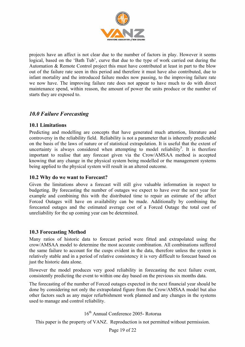
Combining this information with the cost of each Forced Outage, shows that if there had being no improvement of the performance from the 1999 – 2000 period we could have expected to see as much as 150 extra Forced outages in the last year

graphically represented in Figure 11.1. Mby spending more money in direct preventative measures but by utilising the existing resources in different ways. This is born out by the fact that even though the generating output from the fleet and the number of starts those units were asked to perform have increased, the number of staff and the direct maintenance spend has remained constant or dropped. This outcome mirrors well the concept of reliability growth management, which is defined as, “The systematic planning for reliability achievement as a function of time and other

achievemresources, and controlling the ongoing rate of o



of 22

Savings

Figure 11.1

If further reduction in the number of Forced Outages is desired, bearing in mind the potential savings, then any improvement can either be made by further controlling the ongoing rate of achievement by reallocating of existing resources based on comparison between planned and assessed reliability values or by a greater direct spend on maintenance. However any program or physical change to plant designed to reduce the failure rate needs to be done for less cost than the combined value of the ongoing Forced Outages it is expected to save.



of 22

Acknowledgements • Mark Cain, Meridian Energy, Team Leader Asset Coordinators Mid-Waitaki • Terry Smith, Meridian Energy, Business Analyst • Kelvin Jopson, Team Leader Asset Coordinators, Upper -Waitaki

References 1. Abernathy, R ‘The New Weibull Handbook, Forth Edition’, Robert B Abernathy 2000 2. Broeman W, et al, ‘Technical Report No. TR-652 AMSAA Reliability Growth

Guide’, AMSAA 2000 3. ‘Military Handbook – 189 Reliability Growth Management’, US Department of

Defence 1981 4. Barringer P, ‘Problem of the Month, Nov 2002 – Crow/AMSAA Reliability Growth

Plots’ www.barringer1.com, 2003 5. O’Connor, P ‘Practical Reliability Engineering, Forth Edition’ Wiley, 2002

crow amsaa

Documents

constant reliability

projecting reliability

crowamsaa technique

crowamsaa plots

main unit failure data

crowamsaa model

failure rates

event analysis system