cross validation of the gambling problem severity … · original paper cross validation of the...
TRANSCRIPT

ORI GIN AL PA PER
Cross Validation of the Gambling Problem SeveritySubscale of the Canadian Adolescent Gambling Index(CAGI/GPSS) on a Sample of Ontario High SchoolStudents
Nigel E. Turner1,2• Tara Elton-Marshall1,2,3
• Jing Shi1,4•
Jamie Wiebe5• Angela Boak1
• Mark van der Maas1•
Robert E. Mann1,2
Published online: 28 November 2017� The Author(s) 2017. This article is an open access publication
Abstract This paper reports on the cross validation of the Gambling Problem Severity Subscale
of the Canadian Adolescent Gambling Index (CAGI/GPSS). The CAGI/GPSS was included in a
large school based drug use and health survey conducted in 2015. Data from students in grades
9–12 (ages 13–20 years) derived from the (N = 3369 students). The CAGI/GPSS produced an
alpha of 0.789. A principle component analysis revealed two eigenvalues greater than one. An
oblique rotation revealed these components to represent consequences and over involvement.
The CAGI/GPSS indicated that 1% of the students fell into the ‘‘red’’ category indicating a
severe problem and an additional 3.3% scored in the ‘‘yellow’’ category indicating low to
moderate problems. The CAGI/GPSS was shown to be significantly correlated with gambling
frequency (r = 0.36), largest expenditure (r = 0.37), sex (more likely to be male) (r = -0.19),
lower school marks (r = -0.07), hazardous drinking, (r = 0.16), problem video game play
(r = 0.16), as well as substance abuse. The CAGI/GPSS was cross validated using a shorted
version of the short SOGS, r = 0.48. In addition the CAGI/GPSS and short SOGS produced
very similar patterns of correlations results. The results support the validity and reliability of the
CAGI/GPSS as a measure of gambling problems among adolescents.
Keywords Adolescent gambling � Problem gambling � Psychometrics
properties � School survey
& Nigel E. [email protected]
1 Institute for Mental Health Policy Research, Centre for Addiction and Mental Health, 33 RussellStreet, Toronto, ON M5S 2S1, Canada
2 Dalla Lana School of Public Health, University of Toronto, Toronto, ON, Canada
3 Department of Epidemiology and Biostatistics, Western University, London, ON, Canada
4 Rehabilitation Science Institute, University of Toronto, Toronto, ON, Canada
5 Responsible Gambling Council, Toronto, ON, Canada
123
J Gambl Stud (2018) 34:521–537https://doi.org/10.1007/s10899-017-9731-1
Introduction
Adolescents are often viewed as being particularly vulnerable to gambling-related harms
(Gupta and Derevensky 1998a; Shaffer et al. 1999; Turner et al. 2008a). Previous studies of
gambling among adolescents found that as many as 80% of adolescents engage in some
form of gambling and that they participate in a wide variety of gambling activities (Elton-
Marshall et al. 2016; Gupta and Derevensky 1998b; Turner et al. 2011, 2008a, b). Given
that most commercial gambling has age restrictions, much of the gambling among ado-
lescents takes the form of private bets. Some studies of the prevalence of problem gam-
bling among adolescents have found the rate is two to three times higher than that of adults
(Gupta and Derevensky 1998a; Ladouceur 1996; Shaffer and Hall 2001; Shaffer et al.
1999; Turner et al. 2008a; Wiebe et al. 2005). Furthermore, research shows that adults with
gambling problems often started to gamble during adolescence (Griffiths 1995; Gupta and
Derevensky 1998b; Kaminer and Petry 1999; Shaffer and Hall 1996; Turner et al. 2006).
Reports of higher prevalence of gambling problems among adolescents have been
challenged by some researchers (Ladouceur et al. 2000; Welte et al. 2008). In particular, it
was argued by Ladouceur et al. (2000) that adolescents endorse items on questionnaires
more often because they do not understand the items (Wiebe et al. 2005). Furthermore,
Wiebe et al. (2005) noted that the estimated prevalence varies from study to study in part
because of differences in the measures and methods used. In addition, these previous
measures were either created for adult with gambling problems or were adapted for ado-
lescents (Wiebe et al. 2005). Tremblay et al. (2010) have recently developed a scale that
was designed specifically for adolescents, called the Gambling Problem Severity Subscale
of the Canadian Adolescent Gambling Index (CAGI/GPSS). The project was sponsored by
the Canadian Centre on Substance Abuse and the Interprovincial Consortium on Gambling
Research.
The development of the CAGI/GPSS was undertaken in three phases (Tremblay et al.
2010). The first phase developed a conceptualization and operational definition of
problem gambling specific to the adolescent population, as well as a draft pool of items
for measuring problem gambling (Wiebe et al. 2005). Phase two pilot tested an English
and French version of the pool of items with a sample of adolescents drawn from school
populations in Manitoba and Quebec. This was followed a year later with a larger
sample of 2394 students, a retest of 343 students from the general school survey (Wiebe
et al. 2007), and clinical interviews with 109 students who initially participated in the
general school survey. Phase three fine-tuned cut scores and further validated the
instrument by testing with students at increased risk of having problems with gambling
problems (e.g. adolescents who were receiving treatment for substance abuse or were
receiving services from youth centres) or who were currently experiencing problems
with gambling and were classified as pathological gamblers based on clinician ratings
(Tremblay et al. 2010). The CAGI scores were compared to the clinicians ratings
(Tremblay et al. 2010).
The final version of the CAGI consists of 24 items covering the consequences of
gambling/betting. The 24 items are composed of three subscales related to consequences
(psychological, social, and financial), a fourth subscale related to loss of control and a fifth
subscale that measures the global severity of gambling problems. The fifth subscale,
referred to as the Gambling Problem Severity Subscale (GPSS) consists of items from the
three consequences subscales and the loss of control subscale.
As a result of this development process, the CAGI/GPSS was the first problem gambling
measure that was developed specifically for adolescents rather than an adoption of existing
522 J Gambl Stud (2018) 34:521–537
123

instruments developed and tested on adults (Stinchfield 2010).1 The CAGI/GPSS is similar
to the Canadian Problem Gambling Index that was developed by Ferris and Wynne (2001)
for adults, in that it is designed to provide a continuum of problem gambling severity
(Stinchfield 2010) from non-problem gambling to high risk problem gambling. The nine-
item Gambling Problem Severity Subscale (GPSS) of the CAGI is designed to categorize
gambling into ‘‘no problem gambling,’’ ‘‘low to moderate severity,’’ and ‘‘high severity.’’
Although the scale is based on a solid research foundation (Edgren et al. 2016), there is
currently a lack of research cross validating the psychometric properties of this scale,
comparing the scale to an existing measure of gambling problems, and few studies have
examined the factors associated with problem gambling as measured by this scale.
The current study examines problem gambling among a representative sample of
adolescents in the province of Ontario, using data from the 2015 Survey Ontario Student
Drug Use Heath Survey (OSDUHS; Boak et al. 2015). This is one of the first studies to use
the CAGI/GPSS in a general population survey of adolescents. This study therefore pro-
vides a valuable opportunity to test the internal validity and external validity of the CAGI/
GPSS and to compare the CAGI/GPSS to another measure of problem gambling among
youth (the Short South Oaks Gambling Screen).
Methods
Sample
Data from students in grades 9–12 (ages 13–20 years) derived from the 2015 cycle of the
OSDUHS survey were analyzed. The OSDUHS, conducted every 2 years since 1977, is
funded by the Ontario Ministry of Health and Long Term Care and is the longest ongoing
school study of adolescents in Canada. This cross-sectional, anonymous in-class survey,
which employs a regionally-stratified, two-stage cluster (school, class) sampling design,
monitors substance use, mental and physical health, and risk behavior among students in
grades 7–12 in Ontario. The 2015 cycle was based on a total sample of 10,426 pupils in
220 publicly funded elementary/middle and secondary schools. The gambling problem
scales were contained in half the questionnaires developed for high school students only
(grades 9–12), which were randomly distributed within each classroom resulting in a
sample of 3426 high school students. Of these, 57 (1.7%) were excluded because of
missing information on measures used in this study, resulting in a final sample size of 3369
students.
The questionnaires were administered by staff from the Institute for Social Research,
York University on a classroom basis. Students recorded their responses directly onto the
questionnaire forms and were instructed not to write their names on the forms. The student
participation rate was 60% for high school students. Reasons for student non-completion
included absenteeism (11%) and absence of parental consent (29%). The questionnaires
were administered between November 2014 and June 2015. Institutional research ethics
committees at Centre for Addiction and Mental Health, York University, as well as at 30
district school boards approved this study. Further study details are provided in Boak et al.
(2015).
1 There has since been a scale published in Korean that was developed for adolescents by Park and Jung(2012). Park and Jung’s scale however does not appear to have been calibrated to measure disorderedgambling.
J Gambl Stud (2018) 34:521–537 523
123

Measures
Problem Gambling
Problem gambling was measured using two scales. The Gambling Problem Severity
Subscale from the Canadian Adolescent Gambling Index (CAGI/GPSS) and a shortened
version of the South Oaks Gambling Screen Revised for Adolescents (SOGS-RA), referred
to as the short SOGS. The GPSS consists of nine items (see Table 1) scores on 4 point
scale from 0 to 3, and then a total score was computed (see note in Table 1). The nine
CAGI/GPSS items were scored from 0 to 3, for a total score ranging from 0 to 27
(Tremblay et al. 2010). The total score was then categorized as 0–1 = No problem (green
light), 2–5 = a Low-to-moderate severity (yellow light), and 6? = High severity (red
light) (Tremblay et al. 2010). Never gambled and never gambled in past 3 months were
coded as 0. The short SOGS was created from the SOGS-RA due to space limitations in the
survey several years ago. The short SOGS is a list of six gambling symptoms that were
taken from the SOGS-RA (Winters et al. 1993). Six items were selected to maximize the
content and variance of the full SOGS-RA with a minimum of items (Adlaf and Paglia-
Boak 2003; Cook et al. 2015). The items were each scored as 1 for yes and 0 for no for a
total score ranging from 0 to 6. The short SOGS has a coefficient alpha measuring internal
consistency of alpha = 0.71 (Adlaf and Paglia-Boak 2003). Gambling activities were
measured by a series of 11 questions about frequency of participation in various gambling
activities and one question on overall expenditure.
Table 1 Gambling Problem Severity Subscale from the Canadian Adolescent Gambling Index (CAGI/GPSS) severity scale items-total statistics for CAGI/GPSS items
In the last 3 months… Item-totalcorrelation
Alpha if itemdeleted
(1) How often have you skipped practice or dropped out of activities(such as team sports or band) due to your gambling
0.422 0.776
(2) How often have you skipped hanging out with friends who do notgamble to hang out with friends who do gamble?
0.574 0.762
(3) How often have you planned your gambling activities? 0.327 0.813
(4) How often have you felt bad about the way you gamble? 0.600 0.755
(5) How often have you gone back another day to try to win back themoney you lost while gambling?
0.616 0.747
(6) How often have you hidden your gambling from your parents, otherfamily members, or teachers?
0.520 0.766
(7) How often have you felt that you might have a problem withgambling?
0.643 0.755
(8) How often have you taken money that you were supposed to spend onlunch, clothing, movies, etc., and used it for gambling or for paying offgambling debts?
0.526 0.765
(9) How often have you stolen money or other things of value in order togamble or to pay off your gambling debts?
0.409 0.783
For items 1–7 the scale was scored as follows: 0 = Never, 1 = Sometimes, 3 = Most of the time and3 = Almost always. For items 8 and 9, the scale was as follows, 0 = Never, 1 = 1–3 times, 2 = 4–6 times,and 3 = 7 or more times. The total score was the sum of all items responses. The wording of the items hasbeen altered somewhat by removing the words bet and betting from the items to make it easier to read
524 J Gambl Stud (2018) 34:521–537
123

Substance Use and Abuse
Past year cigarette smoking was recorded if the student smoked at least one cigarette daily
or smoked occasionally during the past 12 months (Paglia-Boak et al. 2011). Students who
smoked a few puffs or less than one cigarette in the past 12 months were not classified as
smokers (binary coded as 1 = smokers, 0 = non-smokers). Past year alcohol use was
recorded if the student reported that they consumed any alcohol during the past 12 months
(Paglia-Boak et al. 2011). Students were asked if they used cannabis at least once during
the past 12 months (binary coded as 1) (Paglia-Boak et al. 2011).
To measure substance problem use, the questionnaire included the 6-item CRAFFT2
screener that assesses drug use problems experienced by adolescents (Knight et al. 2002).
The six yes/no items pertain to problems experienced during the past year. Those endorsing
two or more symptoms (binary coded as 1) identified adolescents as having a drug use
problem. Hazardous and harmful drinking was used using the Alcohol Use Disorders
Identification Test (AUDIT), which was developed by the World Health Organization
(Saunders et al. 1993). This instrument is designed to detect problem drinkers at the less
severe end of the spectrum of alcohol problems, and has been used in several previous
studies (e.g. Adlaf and Ialomiteanu 2000; Turner et al. 2011). Those with a score of eight
or more (out of 40) are considered to be drinking at a hazardous or harmful level. The
reliability coefficient (a) for these items is 0.87.
Sociodemographic and Other Correlates
Sociodemographic correlates included: sex, grade, ethno-racial background, self-estimated
current average school marks (Paglia-Boak et al. 2011) and problem video game play
assessed using The Problem Videogame Playing (PVP) scale (Tejeiro Salguero and Moran
2002).
Data Analysis
Descriptive analyses of the CAGI/GPSS were used to calculate the reliability, component
structure, and correlates of the GPSS. In addition we computed an estimate of the
prevalence of moderate and severe problems (yellow and red) assuming the cut off points
recommended by Tremblay, et al. (2010). In addition, Chi-square analyses were used to
examine GPSS scores by sex, grade, ethno-racial background, and school grades. All
analyses were conducted using Stata 11.0 (StataCorp 2009).3
2 CRAFFT stands for the 6 items of the scale: Car, Relax, Alone, Forget, Friends, Trouble.3 The data was collected using a complex design where the schools were randomly selected, and thestudents were nested within classes that were nested within schools. Typically weights are used due to theunequal probabilities of selection as well as post-stratification weights adjusting for sex and grade to ensurethat the sample is representative of the entire provincial student population in publicly funded schools.However, in this paper we are not interested in generalizing to the hypothetical population but are moreinterested in the quality of the items themselves and the individual participants, so these analyses were notweighted so that each person’s data only represented him or herself.
J Gambl Stud (2018) 34:521–537 525
123
Results
In total 3369 participants completed the CAGI questionnaire; 26.8% in Grade 9, 25.8% in
Grade 10, 23.6% in Grade 11, and 23.8% in Grade 12. The sample was 54.4% female and
45.6% male. The majority of students (58.6%) estimated their grade average to be in the A
range (80–100%). For ethnic self-identification, White was the most popular category at
69.9% followed by one of the East or Southeast Asian categories (12.8%), South Asian
(7.5%), Black (7.5%), Aboriginal/First Nations (4.0%), Latin American (3.8%), West
Asian/Arab (3.4%) and ‘‘not sure’’(1.4%).
Gambling Problem Severity Subscale of the CAGI
The Gambling Problem Severity Subscale (CAGI/GPSS) consists of nine items shown in
Table 1. The reliability of these items is good with an alpha of 0.789. As shown in Table 1
the item total correlations ranged from 0.33 to 0.53; the alpha if deleted suggested
improving the alpha score if one item was deleted, but only slightly to 0.81 from 0.79.
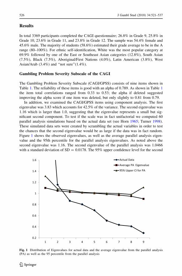
In addition, we examined the CAGI/GPSS items using component analysis. The first
eigenvalue was 3.83 which accounts for 42.5% of the variance. The second eigenvalue was
1.16 which is larger than 1.0, suggesting that the eigenvalue represents a small but sig-
nificant second component. To test if the scale was in fact unifactorial we computed 60
parallel analysis simulations based on the actual data set (see Horn 1965; Turner 1998).
These simulated data sets were created by scrambling the actual variables in order to test
the chances that the second eigenvalue would be as large if the data was in fact random.
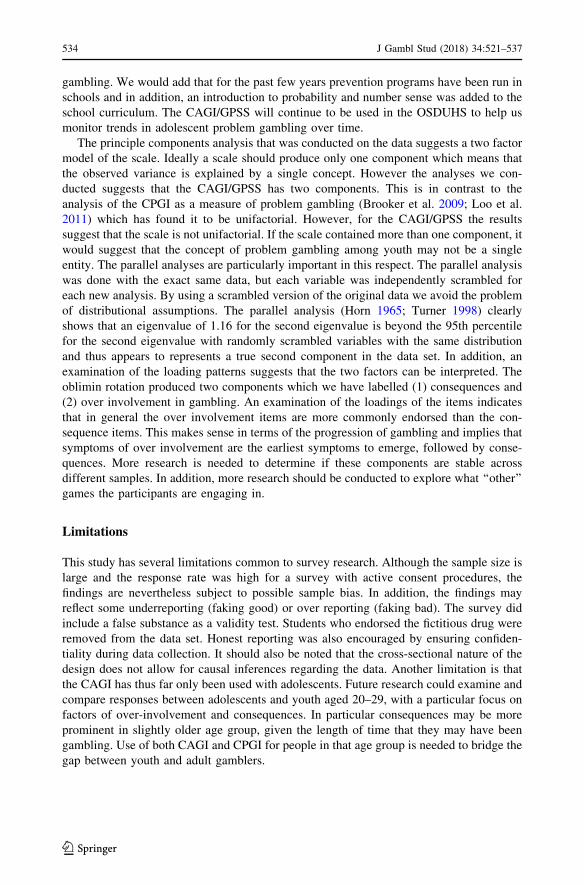
Figure 1 shows the observed eigenvalues, as well as the average parallel analysis eigen-
value and the 95th percentile for the parallel analysis eigenvalues. As noted above the
second eigenvalue was 1.16. The second eigenvalue of the parallel analysis was 1.0466
with a standard deviation of SD = 0.0178. The 95% upper confidence level for the second
0.2
0.4
0.6
0.8
1
1.2
1.4
1.6
1 2 3 4 5 6 7 8 9
Actual Data
Average PA Eigenvalue
95% Upper CI for PA
Fig. 1 Distribution of Eigenvalues for actual data and the average eigenvalue from the parallel analysis(PA) as well as the 95 percentile from the parallel analysis
526 J Gambl Stud (2018) 34:521–537
123

eigenvalue was computed to be 1.0815 which is well below the size of the second observed
eigenvalue in the real data, 1.16, indicating that the second eigenvalue represents real
common variance.
Both varimax and oblimin rotations were conducted for the two components. These two
analyses produced very similar components, but the oblimin was somewhat cleaner. The
oblimin (delta = 0.1) rotation is shown in Table 2. The correlation between the compo-
nents was rho = 0.55. The first component had the highest loadings on item 2 (skipped
hanging out with friends), item 9 (stolen money) and item 1 (skipped practice or dropped
out of activities) and could be interpreted as representing consequences of problem
gambling. The second component has the highest loadings on item 6 (hiding gambling
from family), item 5 (trying to win back money) and item 1 (skipped practice or dropped
out of activities) and could be interpreted as a component representing over involvement in
gambling. Item 7 (felt you might have a problem with gambling) had nearly equal weak
loadings on component 1 (0.31) and component 2 (0.28). Item 8 (spending lunch money
gambling) only had a weak loading of 0.30 on component 1. Note that removing the item
with the lowest item total correlation, item 3 (see Table 1), did not alter the factor
structure.
Table 3 presents the means, standard deviations, and endorsement patterns for the 9
CAGI/GPSS items (coded from 0 = never to 3 = always). An examination of the indi-
vidual items indicates that the items vary from a mean of 0.060 for item 3 to a low of 0.007
for item 9. In particular 24 students endorse ‘‘always’’ for time 3, whereas only one student
Table 2 Oblimin rotation of CAGI/GPSS items
Factor1
Factor2
Component 1: consequences
(2) How often have you skipped hanging out with friends who do not gamble/bet tohang out with friends who do gamble?
0.53 0.01
(9) How often have you stolen money or other things of value in order to gamble/bet orto pay off your gambling debts?
0.51 - 0.08
(1) How often have you skipped practice or dropped out of activities (such as teamsports or band) due to your gambling?
0.48 - 0.04
(7) How often have you felt that you might have a problem with gambling? 0.31 0.28
(8) How often have you taken money that you were supposed to spend on lunch,clothing, movies, etc., and used it for gambling/betting or for paying off gamblingdebts?
0.30 0.19
Component 2: over involvement
(6) How often have you hidden your gambling from your parents, other familymembers, or teachers?
- 0.06 0.53
(5) How often have you gone back another day to try to win back the money you lostwhile gambling?
0.01 0.52
(3) How often have you planned your gambling activities? - 0.12 0.43
(4) How often have you felt bad about the way you gamble? 0.16 0.38
These loadings are computed by Stata 11.0 (StataCorp 2009) which presents them differently than SPSS. InStata the sum of all squared loadings equal 1.0 whereas in SPSS the sum of all squared loading equal theeigenvalue. As a result these weights in Stata are smaller than the equivalent weights in SPSS (e.g. a Stataloading of 0.5 could be equivalent to an SPSS loading of 0.7 or 0.8)
J Gambl Stud (2018) 34:521–537 527
123
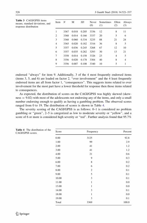
endorsed ‘‘always’’ for item 9. Additionally, 3 of the 4 most frequently endorsed items
(items 3, 5, and 6) are loaded on factor 2, ‘‘over involvement’’ and the 4 least frequently
endorsed items are all from factor 1, ‘‘consequences’’. This suggests items related to over
involvement for the most part have a lower threshold for response then those items related
to consequences.
As expected, the distribution of scores on the CAGI/GPSS was highly skewed (skew-
ness = 9.02) with most of the adolescents not endorsing any of the items, and only a small
number endorsing enough to qualify as having a gambling problem. The observed scores
ranged from 0 to 19. The distribution of scores is shown in Table 4.
The severity scoring of the CAGI/GPSS is as follows: 0–1 is considered no problem
gambling or ‘‘green’’, 2–5 is categorized as low to moderate severity or ‘‘yellow’’, and a
score of 6 or more is considered high severity or ‘‘red’’. Further analysis found that 95.7%
Table 3 CAGI/GPSS itemsmeans, standard deviations, andresponse distribution
Item N M SD Never(0)
Sometimes(1)
Often(2)
Always(3)
1 3367 0.018 0.205 3336 12 8 11
2 3368 0.014 0.166 3337 20 5 6
3 3368 0.060 0.334 3235 88 21 24
4 3365 0.020 0.182 3316 36 8 5
5 3357 0.036 0.245 3268 67 12 10
6 3357 0.035 0.282 3293 30 13 21
7 3358 0.014 0.158 3326 23 4 5
8 3356 0.020 0.178 3304 40 8 4
9 3356 0.007 0.108 3340 10 5 1
Table 4 The distribution of theCAGI/GPSS scores
Score Frequency Percent
0.00 3125 92.8
1.00 99 2.9
2.00 41 1.2
3.00 41 1.2
4.00 21 0.6
5.00 9 0.3
6.00 8 0.2
7.00 6 0.2
8.00 2 0.1
9.00 5 0.1
10.00 3 0.1
11.00 1 0.0
13.00 1 0.0
14.00 3 0.1
18.00 1 0.0
19.00 3 0.1
Total 3369 100.0
528 J Gambl Stud (2018) 34:521–537
123

of the students scored as no problem with gambling (green), 3.3% reported some problem
with gambling (yellow), and 1.0% reported having a severe problem with gambling (red).
Short SOGS and CAGI/GPSS Comparisons
A reliability analysis was also conducted on the short SOGS that had been used in the
survey since 1999. The alpha for the current study was 0.51. The item total correlations
were poor compared to the CAGI/GPSS ranging from 0.17 to 0.45. The alpha if deleted
measure, did not suggest removing any of the items on the short SOGS.
We next examined the relationship between the CAGI/GPSS and the short SOGS. The
correlation between the CAGI/GPSS and the short SOGS was Pearson r = 0.478, Spear-
man rho = 0.411. The cut off values for the two scales (2 for the short SOGS and 6 for the
CAGI/GPSS) produced exactly the same estimate of problem gambling prevalence: 1%.
However, there was not a strong overlap in responses to the two scales. As shown in
Table 5, only 12 adolescents were identified as problematic with both scales. The absence
of a true gold standard makes it impossible to determine which adolescents are actually
false positives and which are false negative (e.g. those identified by the short SOGS or
those identified by the CAGI/GPSS). Thus the relationship between the short SOGS and
the CAGI/GPSS categories is unclear.
To further validate the two measures, we examined the relationship of these two scales
to other variables that should be correlated with problem gambling. Spearman correlations
were used to examine the relationships because of the highly skewed nature of the vari-
ables. As shown in Table 6, both the CAGI/GPSS and the short SOGS were significantly
correlated with gambling frequency and largest amount of money spent gambling. The
CAGI/GPSS and short SOGS had similar patterns of correlations with the largest bet and
with the frequency of participation in various games. In nearly all cases, the correlations
for the CAGI/GPSS were somewhat higher than for the short SOGS. The one exception is
for betting on dice where the short SOGS correlation is slightly larger than for the CAGI/
GPSS. It is interesting that the highest correlations of the CAGI/GPSS are for non-com-
mercial games such as card games and games of skill. However, the exception to this is
online forms of gambling.
As shown in Table 6, the most common gambling activities in the 12 months before the
survey were bets on sports pools (11.0%), ‘‘other ways’’ (10.5%), card games (9.8%), and
lottery tickets (8.6%). With the exception of lottery tickets, the most common types of
gambling games are not commercially controlled types of gambling. The least frequently
reported games were bets on casino games in Ontario and video lottery games. This last
point is not surprising because casinos have strictly enforced age restrictions. The two
commercial games that were played the most often are lotteries and bingo; some of the
adolescents are old enough to play these games. Lottery purchases were reported by
between 5 and 7% of the students from Grades 9–11, but jumped to 16.8% in Grade 12 by
Table 5 Comparison of CAGI/GPSS categories with the shortSOGS
0 or 1 yes Yes on 2 or more Total
1.00 green 3203 11 3214
2.00 yellow 103 9 112
3.00 red 21 12 33
Total 3327 32 3359
J Gambl Stud (2018) 34:521–537 529
123

which point many of the students would be legally able to purchase those lottery tickets.
Total gambling frequency was computed by adding up the number of times spent playing
each of the forms of gambling. As shown in Table 7, total frequency had a correlation of
r = 0.36 with the CAGI/GPSS total score and r = 0.24 with the short SOGS. The students
in the green category on the CAGI/GPSS reported gambling on average 2.6 times
(SD = 15.8). The students who fell into the yellow reported gambling 25.5 times
(SD = 55.4), and those in the red category reported gambling 63 times (SD = 160.1) on
average. Largest amount spent gambling was correlated with the CAGI/GPSS scores,
r = 0.37 and r = 0.28 with the short SOGS. Although 6 out of the 29 youth in the red
Table 6 Correlations of the CAGI/GPSS and short SOGS, with the largest bet and gambling frequency(n = 3267)
Variable Participation(%)
CAGI/GPSStotal
ShortSOGS
How often…Bet money on cards games 9.8 0.29 0.22
Bet money on dice games 3.0 0.19 0.22
Bet money on games of skill (pool, darts, bowling,chess)
7.9 0.31 0.26
Played bingo for money 5.3 0.13 0.10
Bet money in sports pools 11.0 0.26 0.17
Bought sports lottery tickets 3.0 0.22 0.19
Bought any other lottery tickets 8.6 0.14 0.13
Bet money at video gambling machines 1.8 0.21 0.18
Bet money at casino in Ontario 0.5 0.11 0.08
Bet money over Internet 4.2 0.28 0.21
Bet money in other ways 10.5 0.17 0.17
Mean (STE)
Largest amount of money spent gambling 0.45 (0.06) 0.37 0.28
Total gambling frequency 6.18 (0.04) 0.36 0.24
All correlations were significant at p\ 0.001
Table 7 Largest amount bet byCAGI/GPSS category
Green Yellow Red
Never gambled in lifetime 1899 8 2 1909
Did not gamble/12 months 239 3 1 243
$1 or less 167 6 2 175
$2–$9 450 28 5 483
$10–$49 287 40 7 334
$50–$99 41 11 6 58
$100–$199 12 7 3 22
$200 or more 15 6 6 27
3111 109 32 3251
530 J Gambl Stud (2018) 34:521–537
123

category reported betting more than $200, 7 reported that their largest bet was less than
$10. In addition, more than half of those who reported spending $200 in a single event,
scored in the Green zone on the CAGI/GPSS. Table 7 shows a breakdown of largest bet by
problem gambling category.
Table 8 displays the correlation of the CAGI/GPSS and the short SOGS as well as
giving a detailed breakdown of the CAGI/GPSS problem gambling categories and
demographic variables. Males were more likely than females to score in the red and yellow
category of the CAGI/GPSS. Younger students were slightly more likely to score in the
‘‘green’’ category compared to older students. Similarly, there was a weak relationship
between ethno-cultural background and problem gambling. Proportionately more of the
non-white students fell into the red category than white students 1.6 versus 0.7%, the
reverse was true for the yellow category 2.4 versus 3.7%. Finally, problem gambling was
higher amongst students who reported lower marks in school where only 0.3% of students
who report getting mostly As, but 9.8% who reported getting mostly Ds, were categorized
as ‘‘red’’. Table 8 also provides the Spearman correlations for these variables with the
CAGI/GPSS and short SOGS. Sex and school marks are linearly correlated with both the
CAGI/GPSS and short SOGS, but the linear component for white versus other and for
grade were not significant.
In addition, we explored variables that have been shown to be related to problem
gambling in previous research. It is well known that people who report one type of
Table 8 Demographic variables and CAGI/GPSS categories
Variables CAGI/GPSS categories Total Correlations
Green(%)
Yellow(%)
Red(%)
CAGI/GPSS
Short-SOGS
Sex
Male 92.1 5.9 1.9 1536 - 0.19*** - 0.12***
Female 98.7 1.1 0.2 1833
Grade level
Grade 9 96.4 2.9 0.8 903 0.04* 0.01
Grade 10 96.4 2.2 1.3 869
Grade 11 94.5 4.8 0.6 795
Grade 12 94.9 3.6 1.2 802
White
No 96.0 2.4 1.6 1014 0.03 0.00
Yes 95.6 3.7 0.7 2355
School marks
Mostly A?: 90–100% 97.2 2.7 0.2 528 0.07*** 0.10***
Mostly As: 80–89% 96.5 3.1 0.3 1443
Mostly Bs: 70–79% 94.9 3.7 1.4 1127
Mostly Cs: 60–69% 92.9 4.5 2.7 225
Mostly Ds and Fs: 59% andbelow
87.8 2.4 9.8 37
Sample size varies slightly from question to question due to missing values. Only 3 students reported gradesof F, so they have been combined with those who reported getting mostly D’s; *p\ 0.05; ***p\ 0.001
J Gambl Stud (2018) 34:521–537 531
123
addiction are also more likely to report having problems with other addictive behaviors. As
shown in Table 9, both the total CAGI/GPSS score and the short SOGS are weakly
correlated with a number of other addictive behaviors. Spearman correlations were used
due to the skewed nature of these variables. The highest correlations are for the GPSS with
the AUDIT, rho = 0.16, and the GPSS with the PVP rho = 0.16. The pattern of corre-
lations is very similar for the two measures of gambling problems, but the correlations for
the CAGI/GPSS total are slightly higher likely due to its superior reliability. For example,
the AUDIT has correlations of rho = 0.16 with the GPSS and rho = 0.13 with the short
SOGS. The similarities in the correlations indicate that the two measures are parallel.
These correlations are weak correlations, but are consistent with the general findings in the
literature.
Discussion
The CAGI/GPSS is the first problem gambling scale designed specifically for adolescents
(Tremblay et al. 2010) and therefore has the potential to be adopted for research examining
adolescent problem gambling. However, prior to wide adoption there is a need for evidence
demonstrating the validity and reliability of the scale and demonstrating whether the scale
is superior to existing measures used for evaluating adolescent problem gambling. This
study demonstrated that the CAGI/GPSS has an adequate level of reliability and in general
the psychometric properties of the CAGI/GPSS are promising. The Cronbach alpha was
0.79 which is high. The item analysis indicated that the items had strong item total
correlations. However, the alpha if deleted did indicate that if item 3 was deleted, the scale
would have a slightly higher reliability of 0.813. This is in spite of the fact that the item had
a respectable item total correlation of 0.33. The item in question was ‘‘How often have you
planned your gambling activities?’’ This item attempts to measure preoccupation may be
somewhat ambiguous because planning gambling does not necessarily mean excessive
gambling. For example, someone making sports bets, will study the teams past perfor-
mances in order to determine which team to bet on. Such behavior is not necessarily
problematic. Thus item 3 may have skewed the results of the severity scale towards people
who participate in games of skill. But at the same time young male problem gamblers most
often are in fact playing games of skill or betting on sports, and many overestimate their
level of skill in these games.
Table 9 Spearman correlations of the CAGI/GPSS total score with other measures of addiction problems
Variable CAGI/GPSStotal
ShortSOGS
CRAFFT scale sum score measuring substance abuse 0.14 0.13
AUDIT scale sum score measuring hazardous drinking 0.16 0.13
Smoked tobacco cigarettes in the past 12 months 0.13 0.09
Drank alcohol in the past 12 months 0.11 0.08
Used cannabis (marijuana or hashish) at least once in the past 12 months 0.11 0.10
Problem video game play (PVP) 0.16 0.14
All correlations are significant at the p\ 0.001 level
532 J Gambl Stud (2018) 34:521–537
123

Overall, the pattern of findings suggests that adolescents in the ‘‘low to moderate’’ and
‘‘high severity’’ categories are distinct therefore lending further credibility to the utility of
the CAGI/GPSS as a measure for detection of problem gambling. In addition, the pattern of
findings in terms of demographic variables (e.g. sex, grade) and comorbidities (e.g. alcohol
problem use, smoking) is consistent with previous research regarding correlates of problem
gambling. In additional the short SOGS and CAGI/GPSS produced similar results with the
CAGI/GPSS yielding slightly higher correlations than the ShortSOGS in general. What is
surprising is that the CAGI/GPSS and the shortSOGS yielded very similar prevalence
estimates in spite of having a relatively small overlap. Only 11 individuals were identified
as having a severe problem by both scales. More research is needed in order to determine
which scale is more accurately identifying the problem gamblers or if the scale need to be
refined to improve its accuracy.
In this study it was found that 1% of adolescents were identified as ‘‘high severity’’ and
a further and 3.3% were ‘‘low to moderate for a combined total of 4.3% as measured by the
CAGI/GPSS. The prevalence figures reported in this study are within the range found for
adolescent gambling problems (0.2–12.3%) in a recent review (Calado et al. 2016). Both
the short SOGS and the CAGI/GPSS produced an estimate of 1% of the youth who scored
in the severe problem range (red light) and of an estimate of 3.3% in the yellow light
category. These figures are lower than in previous studies (Gupta and Derevensky 1998a;
Shaffer et al. 1999), including a recent study of adolescents (Elton-Marshall et al. 2016)
which reported a prevalence of 1.7% severe problem and 3.5% moderate problem gamblers
for a combined total of 5.3% (computed by combining figures from Tables 3, 5). However,
this study examined problem gambling rates among adolescents in three provinces (On-
tario, Newfoundland, and Saskatchewan) whereas the current study examined problem
gambling prevalence in Ontario; therefore differences may be attributable to differences in
the populations sampled.
Nonetheless, the prevalence figures in the current study are toward the higher end of that
previously found for adult problem gambling prevalence which ranges from 2.0 to 3.0% for
the combination of moderate and severe problem gambling and from 0.5 to 1.0% for severe
problem gambling (Cox et al. 2005; Williams et al. 2012). Thus the results of our study are
consistent with previous research demonstrating higher problem gambling prevalence
amongst adolescents compared to adults identified in previous studies (Gupta and
Derevensky 1998a; Shaffer et al. 1999) but only provides at best weak support for the
hypothesis that adolescents are more vulnerable to problem gambling (Gupta and
Derevensky 1998b; Turner et al. 2008a). Further study is needed to determine the distri-
bution of CAGI/GPSS scores in the adolescent population.
Additionally, it’s possible that the lower prevalence rate of 1%, which was found
consistently for both the CAGI/GPSS and the SOGS-RA may be attributable to an actual
decline in the prevalence of problem gambling. Cook et al. (2015) using 2009 data,
reported the short SOGS indicated a prevalence of problem gambling of 2.8%. The
decrease in prevalence is consistent with other studies in Canada that have examined the
rise and fall of problem gambling prevalence in the country (Williams et al. 2012). Wil-
liams et al. (2012) speculate a number of possible reasons for the downward trend
including: (a) increased awareness of potential harms; (b) decreased participation because
the novelty has worn off; (c) the removal of severe problem gamblers from the population
due to severe adverse consequences such as bankruptcy, or suicide; (d) the increased
provision of prevention and treatment resources; as well as other factors (Williams et al.
2012, p. 7). Shaffer (2005) has argued that the gradual fall of gambling problem rates is
consistent with the theory that a populations tends to adapt over time to the presence of
J Gambl Stud (2018) 34:521–537 533
123
gambling. We would add that for the past few years prevention programs have been run in
schools and in addition, an introduction to probability and number sense was added to the
school curriculum. The CAGI/GPSS will continue to be used in the OSDUHS to help us
monitor trends in adolescent problem gambling over time.
The principle components analysis that was conducted on the data suggests a two factor
model of the scale. Ideally a scale should produce only one component which means that
the observed variance is explained by a single concept. However the analyses we con-
ducted suggests that the CAGI/GPSS has two components. This is in contrast to the
analysis of the CPGI as a measure of problem gambling (Brooker et al. 2009; Loo et al.
2011) which has found it to be unifactorial. However, for the CAGI/GPSS the results
suggest that the scale is not unifactorial. If the scale contained more than one component, it
would suggest that the concept of problem gambling among youth may not be a single
entity. The parallel analyses are particularly important in this respect. The parallel analysis
was done with the exact same data, but each variable was independently scrambled for
each new analysis. By using a scrambled version of the original data we avoid the problem
of distributional assumptions. The parallel analysis (Horn 1965; Turner 1998) clearly
shows that an eigenvalue of 1.16 for the second eigenvalue is beyond the 95th percentile
for the second eigenvalue with randomly scrambled variables with the same distribution
and thus appears to represents a true second component in the data set. In addition, an
examination of the loading patterns suggests that the two factors can be interpreted. The
oblimin rotation produced two components which we have labelled (1) consequences and
(2) over involvement in gambling. An examination of the loadings of the items indicates
that in general the over involvement items are more commonly endorsed than the con-
sequence items. This makes sense in terms of the progression of gambling and implies that
symptoms of over involvement are the earliest symptoms to emerge, followed by conse-
quences. More research is needed to determine if these components are stable across
different samples. In addition, more research should be conducted to explore what ‘‘other’’
games the participants are engaging in.
Limitations
This study has several limitations common to survey research. Although the sample size is
large and the response rate was high for a survey with active consent procedures, the
findings are nevertheless subject to possible sample bias. In addition, the findings may
reflect some underreporting (faking good) or over reporting (faking bad). The survey did
include a false substance as a validity test. Students who endorsed the fictitious drug were
removed from the data set. Honest reporting was also encouraged by ensuring confiden-
tiality during data collection. It should also be noted that the cross-sectional nature of the
design does not allow for causal inferences regarding the data. Another limitation is that
the CAGI has thus far only been used with adolescents. Future research could examine and
compare responses between adolescents and youth aged 20–29, with a particular focus on
factors of over-involvement and consequences. In particular consequences may be more
prominent in slightly older age group, given the length of time that they may have been
gambling. Use of both CAGI and CPGI for people in that age group is needed to bridge the
gap between youth and adult gamblers.
534 J Gambl Stud (2018) 34:521–537
123

Conclusion
The current study supports the validity and reliability of the CAGI/GPSS as a measure of
adolescent problem gambling. However, additional research investigating the component
structure of the CAGI is needed to determine the replicability of the two component
structure found in the current study. In addition, the CAGI/GPSS was correlated with
greater involvement in gambling as measured by gambling activities, frequency of play,
and largest bet supporting the CAGI/GPSS’s external validity. In terms of validity the
CAGI/GPSS produced findings that were consistent with previous measures of problem
gambling including higher rates amongst males, higher rates for students with lower school
marks, as well as positive correlations with other problems and risk behaviours.
Funding Funding for this project was based on Grant #06703 from the Ministry of Health and Long TermCare (MHLTC). The ideas expressed are those of the authors and do not necessarily reflect those ofMHLTC, the Centre for Addiction and Mental Health, or the University of Toronto.
Author’s Contribution NT and TEM suggested adding the CAGI/GPSS items to the OSDHUS survey. ABadded the items set up the survey. RM approved the addition and supervised the overall survey. AB did mostof the data handling for the survey. NT analyzed the data in this report. MvM contributed some additionalanalysis and interpretation. JW contributed to the interpretation of the results. NT, JS and TEM wrote thefirst draft. All authors edited the manuscript.
Compliance with Ethical Standards
Conflict of interest The authors report no conflict of interest. NT has received money from the OntarioLottery and Gaming to scientifically evaluate one of their prevention initiatives, but that project has norelationship to this project. In addition the contract for that project ensures our independence from OLG andour rights to publication.
Ethical Standards All procedures performed in studies involving human participants were in accordancewith the ethical standards of the institutional and/or national research committee and with the 1964 Helsinkideclaration and its later amendments or comparable ethical standards. Institutional research ethics com-mittees at CAMH (as protocol #018/2014-03), York University, as well as at 30 district school boardsapproved this study. Further study details are available at: www.camh.ca/research/osduhs.
Open Access This article is distributed under the terms of the Creative Commons Attribution 4.0 Inter-national License (http://creativecommons.org/licenses/by/4.0/), which permits unrestricted use, distribution,and reproduction in any medium, provided you give appropriate credit to the original author(s) and thesource, provide a link to the Creative Commons license, and indicate if changes were made.
References
Adlaf, E. M., & Ialomiteanu, A. (2000). Prevalence of problem gambling in adolescents: Findings from the1999 Ontario Student Drug Use Survey. Canadian Journal of Psychiatry, 45, 752–755.
Adlaf, E. M., & Paglia-Boak, A. (2003). Ontario student drug use survey. Unpublished raw data.Boak, A., Hamilton, H. A., Adlaf, E. M., & Mann, R. E. (2015). Drug use among Ontario students,
1977–2015: Detailed OSDUHS findings (CAMH research document series no. 41). Toronto, ON:Centre for Addiction and Mental Health.
Brooker, I. S., Clara, I. P., & Cox, B. J. (2009). The Canadian Problem Gambling Index: Factor structure andassociations with psychopathology in a nationally representative sample. Canadian Journal of Beha-vioural Science/Revue canadienne des sciences du comportement, 41(2), 109.
Calado, R., Alexandre, J., & Griffiths, M. D. (2016). Prevalence of adolescent problem gambling: Asystematic review of recent research. Journal of Gambling Studies. https://doi.org/10.1007/s10899-016-9627-5.
J Gambl Stud (2018) 34:521–537 535
123

Cook, S., Turner, N. E., Ballon, B., Paglia-Boak, A., Murray, R., Adlaf, E. M., et al. (2015). Problemgambling among Ontario students: Associations with substance abuse, mental health problems, suicideattempts, and delinquent behaviours. Journal of Gambling Studies, 31(4), 1121–1134.
Cox, B. J., Yu, N., Afifi, T. O., & Ladouceur, R. (2005). A national survey of gambling problems in Canada.Canadian Journal of Psychiatry, 50, 213–217.
Edgren, R., Castren, S., Makela, M., Portfors, P., Alho, H., & Salonen, A. H. (2016). Reliability ofinstruments measuring at-risk and problem gambling among young individuals: A systematic reviewcovering years 2009–2015. Journal of Adolescent Health, 58(6), 600–615.
Elton-Marshall, T., Leatherdale, S. T., & Turner, N. E. (2016). An examination of internet and land-basedgambling among adolescents in three Canadian provinces: Results from the youth gambling survey(YGS). BMC Public Health, 16, 277. https://doi.org/10.1186/s12889-016-2933-0.
Ferris, J., & Wynne, H. (2001). The Canadian problem gambling index: Final report. Ottawa: CanadianCentre on Substance Abuse.
Griffiths, M. (1995). Adolescent gambling. London: Psychology Press.Gupta, R., & Derevensky, J. L. (1998a). Adolescent gambling behaviour: A prevalence study and exami-
nation of the correlates associated with problem gambling. Journal of Gambling Studies, 14(4),319–345. https://doi.org/10.1023/A:1023068925328.
Gupta, R., & Derevensky, J. L. (1998b). An empirical examination of Jacobs’ general theory of addictions:Do adolescent gamblers fit the theory? Journal of Gambling Studies, 14, 17–49. https://doi.org/10.1023/A:1023046509031.
Horn, J. L. (1965). A rationale and test for the number of factors in factor analysis. Psychometrika, 30,179–185.
Kaminer, V., & Petry, N. M. (1999). Gambling behavior in youths: Why we should be concerned. Psy-chiatric Services, 50, 167–168.
Knight, J. R., Sherritt, L., Shrier, L. A., Harris, S. K., & Chang, G. (2002). Validity of the CRAFFTsubstance abuse screening test among adolescent clinic patients. Archives of Pediatrics and AdolescentMedicine, 156(6), 607–614.
Ladouceur, R. (1996). The prevalence of pathological gambling in Canada. Journal of Gambling Studies, 12,129–142.
Ladouceur, R., Bouchard, C., Rheaume, N., Jacques, C., Ferland, F., Leblond, J., et al. (2000). Is the SOGSan accurate measure of pathological gambling among children, adolescents and adults? Journal ofGambling Studies, 16(1), 1–24.
Loo, J. M., Oei, T. P., & Raylu, N. (2011). Psychometric evaluation of the problem gambling severity index-chinese version (PGSI-C). Journal of Gambling Studies, 27(3), 453–466.
Paglia-Boak, A., Adlaf, E. M., & Mann, R. E. (2011). Drug use among Ontario students, 1977–2011:Detailed OSDUHS findings (CAMH research document series no. 32).
Park, H. S., & Jung, S. Y. (2012). Development of a Gambling Addictive Behavior Scale for adolescents inKorea. Journal of Korean Academy Nursing, 42, 957–964. https://doi.org/10.4040/jkan.2012.42.7.957.
Saunders, J. B., Aasland, O. G., Babor, T. F., De la Fuente, J. R., & Grant, M. (1993). Development of theAlcohol Use Disorders Identification Test (AUDIT): WHO collaborative project on early detection ofpersons with harmful alcohol consumption-II. Addiction, 88, 791–804. https://doi.org/10.1111/j.1360-0443.1993.tb02093.x.
Shaffer, H. J. (2005). From disabling to enabling the public interest: Natural transitions from gamblingexposure to adaptation and self-regulation. Addiction, 100, 1227–1229.
Shaffer, H. J., & Hall, M. N. (1996). Estimating the prevalence of adolescent gambling disorders: Aquantitative synthesis and guide toward standard gambling nomenclature. Journal of GamblingStudies, 12, 193–214. https://doi.org/10.1007/BF01539174.
Shaffer, H. J., & Hall, M. N. (2001). Updating and refining prevalence estimates of disordered gamblingbehaviour in the United States and Canada. Canadian Journal of Public Health, 92(3), 168–172.
Shaffer, H. J., Hall, M. N., & Vander Bilt, J. (1999). Estimating the prevalence of disordered gamblingbehavior in the United States and Canada: A research synthesis. American Journal of Public Health,89, 1369–1376. https://doi.org/10.2105/AJPH.89.9.1369.
StataCorp. (2009). Stata statistical software: Release 11.0. College Station, TX: Stata Corporation.Stinchfield, R. (2010). A critical review of adolescent problem gambling assessment instruments. Inter-
national Journal of Adolescent Medicine and Health, 22, 77–93. https://doi.org/10.1515/9783110255690.147.
Tejeiro Salguero, R. A., & Moran, R. M. (2002). Measuring problem video game playing in adolescents.Addiction, 97, 1601–1606.
536 J Gambl Stud (2018) 34:521–537
123

Tremblay, J., Stinchfield, R., Wiebe, J., & Wynne, H. (2010). Canadian Adolescent Gambling Inventory(CAGI) Phase III Final Report. Submitted to the Canadian Centre on Substance Abuse and theInterprovincial Consortium on Gambling Research.
Turner, N. E. (1998). The effect of common variance and loading pattern on random data eigenvalues:Implications for the accuracy of parallel analysis. Education and Psychological Measurement, 58,541–568. https://doi.org/10.1177/0013164498058004001.
Turner, N. E., Ialomiteanu, A., Paglia-Boak, A., & Adlaf, E. M. (2011). A typological study of gambling andsubstance use among adolescent students. Journal of Gambling Issues, 25, 88–107. https://doi.org/10.4309/jgi.2011.25.7.
Turner, N. E., Littman-Sharp, N., & Zangeneh, M. (2006). The experience of gambling and its role inproblem gambling. International Gambling Studies, 6, 237–266. https://doi.org/10.1080/14459790600928793.
Turner, N. E., Macdonald, J., Bartoshuk, M., & Zangeneh, M. (2008a). Adolescent gambling behaviour,attitudes, and gambling problems. International Journal of Mental Health and Addiction, 6(2),223–237. https://doi.org/10.1007/s11469-007-9117-1.
Turner, N. E., Macdonald, J., & Somerset, M. (2008b). Life skills, mathematical reasoning and criticalthinking: A curriculum for the prevention of problem gambling. Journal of Gambling Studies, 24,367–380. https://doi.org/10.1007/s10899-007-9085-1.
Welte, J. W., Barnes, G. M., Tidwell, M., & Hoffman, J. H. (2008). The prevalence of problem gamblingamong U.S. adolescents and young adults: Results from a national survey. Journal of GamblingStudies, 24, 119–133. https://doi.org/10.1007/s10899-007-9086-0.
Wiebe, J., Wynne, H., Stinchfield, R., & Tremblay, J. (2005). Measuring problem gambling in adolescentpopulations: Phase one-report. Submitted for the Canadian Centre on Substance Abuse.
Wiebe, J., Wynne, H., Stinchfield, R., & Tremblay, J. (2007). The Canadian Adolescent Gambling Inventory(CAGI) Phase II Final Report. Submitted for the Canadian Centre on Substance Abuse.
Williams, R. J., Volberg, R. A., & Stevens, R. M. G. (2012). The population prevalence of problemgambling: Methodological influences, standardized rates, jurisdictional differences, and worldwidetrends. Ontario Problem Gambling Research Centre and the Ontario Ministry of Health and Long TermCare.
Winters, K. C., Stinchfield, R. D., & Fulkerson, J. (1993). Toward the development of an adolescentgambling problem severity scale. Journal of Gambling Studies, 9(1), 63–84.
J Gambl Stud (2018) 34:521–537 537
123