Cross-layer scheduling of end-to-end flows using a spectrum server

Chandru RamanRoy YatesNarayan Mandayam

Rutgers University

2

Talk OutlineIntroduction – Cognitive Radio & Spectrum Server

Scheduling of variable rate links

End-to-end scheduling of flows using spectrum server

Fairness and Max-Min Fair Flows

Conclusion

3

The Spectrum DebateWhat everyone agrees on:

Spectrum use is inefficientFCC licensing has yielded false scarcity

Proposed SolutionsSpectrum Property Rights

The triumph of economics

Open Access (Commons)The triumph of technology

4

Open AccessA Technology Panacea

Agile wideband radios will dynamically share a commonsMinor technical rules (power spreading) for transceivers

Systems of end-user devicesSpread spectrum, UWB, MIMO, OFDMShort range communicationsAd hoc multi-hop mesh networks

Evidence: (perceived) success of 802.11 vs. 3G

5

Open Access Needs Radio AgilityRequire radios that can :

DiscoverCooperateSelf-Organize into hierarchical networks

Agility needed at every protocol layerBut cannot predict environments/applications

The Answer? “Cognitive Radios”Optimization Perspective:

Enlarging the space of feasible solutions ⇒ improved performance

6

Cognitive Radio: Modeling Issues

Heterogeneous PHYs:OFDM, UWB, FH, CDMA

Is there a control channel?What are control actions?

7

Spectrum Server

A Simple Spectrum Server

Spectrum Server tells radios to turn OFF/ONRadios use best rate given signal & interference

8

Simple System ModelUsers share a common frequency band

Orthogonal signal dimensions = time slotsTime domain scheduling is used for channelization

Wireless network of L directed links

Links follow ON-OFF transmission schedule over time slotsUse constant transmission power in the ON state

Links employ interference-adaptive modulation/codingLink rate in each time slot depends on interference from other active links

Interference depends on the transmission modemode = subset of links that are ON simultaneously

9

Network with L = 4 linksTransmission mode matrix T:

Transmission modes

1 4

3

2

Transmission mode [1 0 1 0]

(one of 24 possible modes)

1

3

[0 0 0 0 0 0 0 0 1 1 1 1 1 1 1 1] [0 0 0 0 1 1 1 1 0 0 0 0 1 1 1 1][0 0 1 1 0 0 1 1 0 0 1 1 0 0 1 1][0 1 0 1 0 1 0 1 0 1 0 1 0 1 0 1]

tli = 1, if active link l is in mode i

= 0, otherwise.

10

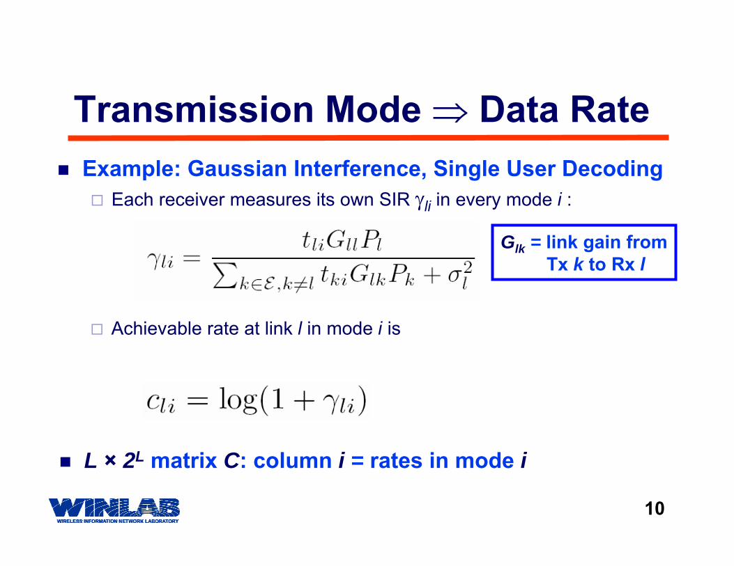
Transmission Mode ⇒ Data RateExample: Gaussian Interference, Single User Decoding

Each receiver measures its own SIR γli in every mode i :

Achievable rate at link l in mode i is

L × 2L matrix C: column i = rates in mode i

Glk = link gain fromTx k to Rx l

11

network with 4 links

Mode Matrix ⇒ Rate Matrix

1 4

3

2

Transmission mode [1 0 1 0]

1

3

Rate matrix C =[6.6 0 0.01 0 0.56 0 0.01 0 2.05[ 0 6.6 0.06 0 0 1.86 0.06 0 0[ 0 0 0 6.6 1.0 1.86 0.83 0 0[ 0 0 0 0 0 0 0 6.65 0.32

0 0.01 0 0.49 0 0.01]0.97 0.06 0 0 0.77 0.06 ]0 0 0.04 0.04 0.04 0.04 ]0.05 0.04 0.40 0.19 0.05 0.04]

12

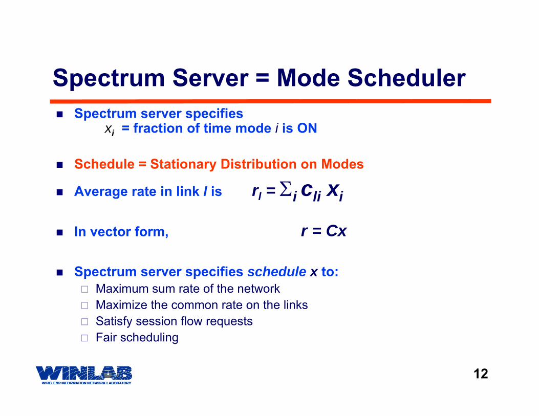
Spectrum server specifies xi = fraction of time mode i is ON

Schedule = Stationary Distribution on Modes

Average rate in link l is rl = Σi cli xi

In vector form, r = Cx

Spectrum server specifies schedule x to:Maximum sum rate of the networkMaximize the common rate on the linksSatisfy session flow requestsFair scheduling

Spectrum Server = Mode Scheduler

13

Average link data rates r = Cx

Any ergodic dynamic spectrum access policy ⇒schedule xaverage link rates r = Cx

Centralized scheduling upperboundsdistributed/dynamic solutions

Tx/Rx technology assumptions are embedded in C

Comments on the Model

14

Technology Modeling Example Duplexing

Duplex constraints in the rate matrix CNode B: Link 1 RX, Link 2 TXG12 = ∞In mode [ 1 1], link 1 gets rate ε0≈ 0, c0 < 1

A B D1 2

A B D

G11 G22G12

G21

0 1 0 ε0

0 0 1 c0C = [ ]

c1

c2

Modes 0 1 2 3

0

2

1

3

Both links ON:link 1 is useless, link 2 is crummy

15

Technology Modeling ExampleIT Multiaccess

Nodes A and B send to DD employs joint decoding

Mode induced by sender code rates & successive decoding order at D

A

BD

1

2

0 1 0 0.5 10 0 1 1 0.5 C = [ ]

c1

c2

Modes 0 1 2 3 4

0

2

1

3

4

16

System model for end-to-end flowsWireless network with N nodes and L linksK end-to-end sessions – a session described by an origin-destination (OD) pairSet of R routes in the networkEnd-to-end route incidence matrix for each flow k:

[Ak]lr = 1, if link l is part of route r= 0, otherwise

Vector fk – session k flows in the R routes

17

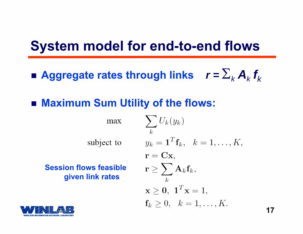
System model for end-to-end flows

Aggregate rates through links r = Σk Ak fk

Maximum Sum Utility of the flows:

Session flows feasiblegiven link rates

18

Cross Layer Optimization??PHY: Link rates cli for each mode iMAC: Schedule x ⇒ Link rates r = CxNetwork: Routes Ak

Transport: Flows fk

r = Cx ≥ Σk Ak fkPHYMAC

NetworkTransport

IssuesDual decomposition methods don’t yield distributed

solutions.xi is not controlled locally by entity i

[Bonald & Proutiere, WP-01]: Flow allocation f drives schedule x

19

Example 1: Max Flow scheduling on a linear network

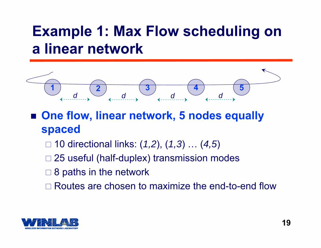
One flow, linear network, 5 nodes equally spaced

10 directional links: (1,2), (1,3) … (4,5)25 useful (half-duplex) transmission modes8 paths in the networkRoutes are chosen to maximize the end-to-end flow

1 2 3 4 5d d d d

20

0 5 10 15 20 25 30 35 40 45 500

2

4

6

8

10

12

Distance between nodes in the network

Sum

rate

of t

he fl

ows

(bits

/sec

/Hz)

Variation of sum of flows with distance

Example 1: Max Flow

1 hop flow, high link SNR

4 hop flow at low SNR

Activity of transmission modes provides the routes

21

Special Case:Session Flows = Link Rates

Each flow traverses one link. Each link carries one flow.Ak = I, fk = rkek,(Session flow) yk = rk (link rate)

22

Max sum link-rate schedulingEach flow traverses one link. Each link carries one flow.

Objective: To maximize the sum rate in the network with minimum rate constraints on each linkOptimization problem can be posed as a linear program

23

Example 2

DistanceAttenuation

⇒Link Gain

24

Maximum sum rate solutionWhen rmin = 0, the dominant mode is always scheduled

Dominant mode – the mode corresponding to the maximum column sum in C

Leads to inherent unfairness in the schedulelinks not active in the dominant mode are never scheduled

25

Example 2: Dominant mode

Dominant mode:the mode that has maximum sum rate

Dominant mode vector is

[0 1 0 0 1]

26

Maximum Sum rate - solution

When each component rmin > 0, more than one mode is used

The disadvantaged links are operated for just enough time to satisfy their rate requirement

Most transmission modes are unused

27

Example 2: As common rmin increases, the sum rate decreasesRates of dominant mode links decreaseRates of disadvantaged links increase

28

Max-min fairnessFlow vector f is max-min fair if fl cannot be increased while maintaining feasibility without decreasing fl’ for some l’ such that fl’ ≤ fl

Example from data networks:

Bottleneck 1C1 = 3

Flow 1

Flow 2Bottleneck 2

C2 = 4

MMF Rates:Flow 1 = 1.5, Flow 2 = 1.5, Flow 3 = 2.5

Flow 3

29

Max-min flow schedule

What is the max-min fair flow schedule in our model?

Step 1: Maximize the minimum flow y using the LP

30

Max-min fair schedule

Theorem: Non-zero link gains ⇒ equal rate flows are max-min fair

Scheduler timeshares between bottlenecks to equalize the user flow ratesThe shared bandwidth is the bottleneck

31

Example 3 – Fair scheduling

f3

Linear network of four nodes, equal link distancesFixed Schedule (Equal link rates)

MMF rates are (f1, f2, f3, f4) = (1/3, 1/3, 1/3, 2/3)

Mode scheduling of links ⇒ equal flowsMMF rates are (f1, f2, f3, f4) = (0.37, 0.37, 0.37, 0.37)

f1

f2f4

r1 = 1 r2 = 1 r3 = 1

32

1 2 3

f1

f2

Example 4: Max-min fair flows(Fixed Mode Schedule)

Spectrum Server Schedule: Link Rates r1 = 10, r2 = 4

f1+f2 ≤ r1

f2 ≤ r2

1 2

33

r2 = 4

r1 = 10

Max-min fair rates (Example)

f1+ f2 ≤ 10f2 ≤ 4

f* = max { min f : f1 ≥ f, f2 ≥ f }

rMMF = (6, 4)

= (4, 4)

f2

f1

34

R2

R1

r2

r1

Rate pair when both links are simultaneously ON

rMMF

MMF rates for the interference model

A

BD

12E

35

Max-min fair schedules“Equal rates are max-min fair” is a property of

flexible (centralized) link schedulingGaussian interference model

[Radunovic & Le Boudec, Infocom 04]Solidarity Property: Decrease in flow i enables strict increase of flow jSolidarity ⇒ equality of max-min fair rates

Solidarity holds for the Gaussian interference model.

36

Solidarity and the C matrixSolidarity depends on the PHY layer (C matrix)

In general, Max Common Rate (MCR) ≠ Max Min Fair (MMF) Rate

AB

D

1

2

A

BD

12E

r1

r2

MMF = MCR

r1

r2

MMFMCR

Interference Model IT MAC Model

37

Concluding remarksSpectrum server computes schedule – time sharing of transmission modes of the networkMaximizing common rate over flows gives the max-min fair flows for the interference modelCentralized scheduler needs to know a lot of information

granularity and timeliness of measurements required by the Spectrum Server will be important

Distributed solutions for finding good PHY layer modes?