Cross-border Investments and Uncertainty: Firm-level Evidence

Rafael Cezar*, Timothée Gigout† and Fabien Tripier‡

April 2020, WP 766

ABSTRACT

This paper studies the impact of uncertainty on cross-border investments. We build a data-set of firm-level outward Foreign Direct Investments between 2000 and 2015. We create a time and country varying measure of uncertainty based on the dispersion of idiosyncratic investment returns. An increase in uncertainty delays cross-border flows to the affected country. Yet, this average e_ect hides strong heterogeneity. Firms with low ex-ante performance durably reduce their foreign investments. Meanwhile high-performing firms increase their investments after the initial shock. We interpret these results as the evidence of a cleansing effect of uncertainty shocks among multinational firms in the presence of financial frictions.∗

Keywords: Uncertainty; Asymmetric Uncertainty; FDI Flows; FDI Returns; Volatility; Multinational Firms.

JEL classification: D81, F23, G10, G15.

* Banque de France, Email: rafael.cezar@banque-france.fr. † Collège de France, Email: timothee.gigoutmagiorani@gmail.com. ‡ EPEE, Univ Evry, Universite Paris-Saclay & CEPII, Email: fabien.tripier@univ-evry.fr. *Acknowledgement: We thank Philippe Aghion, Joshua Aizenman, Jean-Charles Bricongne, Matthieu Bussière, Anne-Célia Disdier, Ludovic Gauvin, Jérôme Hericourt, Jean Imbs, Isabelle Méjean, Gianluca Orefice, Matthias Schoen, Farid Toubal and participants of the Banque de France Phd seminar, CEPII seminar, Paris-Sud Seminar, 23rd Conference on Theories and Methods in Macroeconomics (T2M), 34th SUERF Colloquium/Banque de France, 23rd Annual International Conference on Macroeconomic Analysis and International Finance (ICMAIF), AFSE 2017 and RIEF 2017 conferences. Fabien Tripier acknowledges the financial support of the LabexMME-DII’s grant ANR-11-LBX-0023-01. Working Papers reflect the opinions of the authors and do not necessarily express the views of the Banque de

France. This document is available on publications.banque-france.fr/en

Banque de France WP #766 ii

NON-TECHNICAL SUMMARY

Foreign investors fear uncertainty. This widespread view is repeatedly invoked in the media and political circles during turbulent times as in the current context of Brexit and trade wars. In this paper, we build a measure of uncertainty based on FDI returns of French Multinational Firms (MNF or firms hereafter) to document how FDI react to a rise in uncertainty in the host country. A striking result is the great heterogeneity of the effect of uncertainty on FDI decision. A slightly negative and short-lived average effect hides a strong negative and persistent effect for low-performing MNF which turns out to be positive for high-performing ones. Therefore, besides its moderate effects on average, uncertainty appears as a key driver of reallocation of FDI between MNF. The starting point is to build a microdata based measure of uncertainty for FDI returns. While investigations on the impact of uncertainty on FDI in the literature rely upon global measures of uncertainty as the electoral cycle, the stock market volatility or the exchange rate uncertainty; we investigate herein a measure of uncertainty which is specific to FDI. To get as accurate measure of exogenous uncertainty, we consider the dispersion of FDI returns which are not predicted by relevant factors (Anderson et al. (2009), Boutchkova et al. (2012), Bloom (2014) and Bloom et al. (2018)). More precisely, our uncertainty measure is the standard deviation of the component of FDI returns that is unexplained by its lagged value, the indexes of world and country FDI returns, and an estimated structure of fixed effects. The highest uncertainty is observed in 2008 in Thailand, a year marked by a very serious political crisis. We also observe high values during the Great Recession for several emerging countries (South Africa, India and Romania) and the famous 2001 financial crises in Argentina and Turkey, as well as in Russia (in 2002 and 2006, a year of tensions with Ukraine and international sanctions). Our measurement is therefore a synthetic indicator of the several dimensions of uncertainty (economic, political and financial). We then estimate how FDI react to uncertainty by regressing the individual FDI outflows by French MNF on our measure of uncertainty. We supplement our results with the Local Projection method of Jordà (2005) to assess the persistence of the adverse effect of uncertainty on FDI. Following a one interquartile range increase in uncertainty in one country, French MNF decrease the rate of their direct investments to this affected country by as much as 0:904 points of percentage. Using split sample analysis, we show that this figure hides a strong heterogeneity. Parent companies with low ex-ante performance bear the brunt of the losses from uncertainty and do not experience any recovery in the following years; contrary to parent companies with high ex-ante performance. Indeed, the fall of 0.904 points of percentage of FDI growth on average is associated with a gap of 5.98 points of percentage three years after between parent companies with the highest and the lowest ex-ante performance. In fact, the rise in uncertainty has a positive effect for high-performing parent companies (2.60 ppt) while low-performing firms experienced a dramatic fall in FDI (-3.38 ppt). The small and short-living average effect hides strong and persistent heterogeneous effects of uncertainty on FDI. Our results contribute to the large literature on the relation between FDI and uncertainty, confirming the importance of the effect of uncertainty not only on the aggregate level of FDI flows but also on the composition of the MNF at the origin of those flows. Our results contribute also to literature on the heterogeneous effects of uncertainty shocks. Our contribution is to extend the set of results that highlight the importance of heterogeneity in trade flows to FDI flows; and to identify the role of firms returns as a key source of heterogeneous responses of MNF to uncertainty. Finally, it is worth emphasizing that heterogeneity concerns the sign of the impact and not only its magnitude: the impact of uncertainty is positive for high performing firms. Such effect has also been identified in the

Banque de France WP #766 iii

literature mainly by showing that investment lags in somes spécific sectors - such as R&D, oil and gas or mining - reverse the standard result of the literature on adverse effects of uncertainty on investment. FDI may thus share some features with these types of investment which would explain why they react positively with uncertainty for the most performing firms in our sample.

Investissements transfrontaliers et incertitude : évidence au niveau des firmes

RÉSUMÉ Ce papier examine l’impact de l’incertitude sur les investissements transfrontaliers. Nous construisons une base de données sur les investissements directs étrangers sortants au niveau des firmes entre 2000 et 2015. Nous créons ensuite une mesure de l’incertitude variant en fonction du temps et des pays, basée sur la dispersion des rendements idiosyncrasiques des investissement. Une hausse de l’incertitude retarde les flux transfrontaliers vers le pays concerné. Pourtant, cet effet moyen cache une forte hétérogénéité. Les entreprises dont les performances ex-ante sont faibles réduisent durablement leurs investissements à l’étranger. En parallèle, les entreprises plus performantes augmentent leurs investissements après le choc initial. Nous interprétons ces résultats comme la preuve d’un effet assainissant des chocs d’incertitude parmi les firmes multinationales en présence de frictions financières.

Mots-clés : incertitude ; incertitude asymétrique ; flux d’IDE ; rendement des IDE ; volatilité ; firmes multinationales Les Documents de travail reflètent les idées personnelles de leurs auteurs et n'expriment pas nécessairement

la position de la Banque de France. Ils sont disponibles sur publications.banque-france.fr

1 Introduction

"Brexit fear hits foreign direct investment." Financial Times, 2016

"This uncertainty on where we are going in regards to trade policy and Nafta has

put some international investment in a holding pattern." C. Camacho, President and

CEO of the Greater Phoenix Economic Council. Financial Times, 2017

Foreign investors fear uncertainty. This widespread view is repeatedly invoked in the media

and political circles during turbulent times as in the current context of Brexit and trade wars.

In this paper, we build a measure of uncertainty based on FDI returns of French Multinational

Firms (MNF or firms hereafter) to document how FDI react to a rise in uncertainty of FDI

returns in the host country. A striking result of our empirical analysis is the great heterogeneity

of the effect of return uncertainty on FDI decision. A slightly negative and short-lived average

effect hides a strong negative and persistent effect for low-performing MNF which turns out to

be positive for high-performing ones. Therefore, besides its moderate effects on average, FDI

uncertainty appears as a key driver of reallocation of foreign direct investments between MNF.

The starting point of our paper, and our first contribution to the literature, is to build a micro-

data based measure of uncertainty for FDI returns. While investigations on the impact of un-

certainty on FDI in the literature rely upon global measures of uncertainty as the electoral cycle

(e.g. Julio and Yook (2016)), the stock market volatility (e.g. Gourio et al. (2016)) or the ex-

change rate uncertainty (e.g. Jeanneret (2016)), we investigate herein a measure of uncertainty

which is specific to FDI. Our measure presents the advantage of being more directly connected

with the FDI’s decision. To build this measure, we construct a novel affiliate-level data-set of

French outward FDI flows and assets abroad.1 This data-set allows us to compute the entire

distribution of FDI returns for almost all French MNF over the 2000-2015 sample period.

The standard deviation of FDI returns distribution is informative about the realized risk of

FDI, but it cannot be used directly as a measure of exogenous FDI uncertainty. As empha-

sized by Bloom (2014), exogenous fluctuations in uncertainty are not directly observable and1Vicard (2018) also uses the Banque de France databases to measure FDI returns to study the role of corporate

tax avoidance.

1

we therefore have to rely on necessarily imperfect proxies. By looking at the width of the dis-

tribution of the reasonably unpredictable component of those outcomes, we get closer to the

true notion of uncertainty as Jurado et al. (2015) point out. To get a more accurate measure

of uncertainty, we then consider the dispersion of FDI returns which are not predicted by rele-

vant factors. The selected factors are borrowed from the literature in finance on idiosyncratic

volatility of returns. Whereas Ang et al. (2006) and Ang et al. (2009) use a multiple French

and Fama Factors model to predict idiosyncratic returns, it is also possible to employ a more

parsimonious model as in Anderson et al. (2009) and Boutchkova et al. (2012). In that set-up,

firms’ returns are typically regressed over two indexes of country and global returns with some

fixed effects accounting for firm invariant characteristics. We also borrow to the literature on

uncertainty measures based on firm-level data exposed in Bloom (2014) and more precisely

Bloom et al. (2018) who apply auto-regressive models to the establishment-level measure of

productivity to identify uncertainty shocks on firm productivity. Therefore, our measure of

uncertainty is defined as the standard deviation of the component of FDI returns which is unex-

plained by the lagged value of FDI returns, the indexes of world and country FDI returns, and

an estimated structure of fixed effects.

Our measure of uncertainty is time-varying with cross-country and cross-sectoral dimen-

sions.2 The highest uncertainty is observed in 2008 in Thailand, a year marked by a very

serious political crisis.3 We also observe high values during the Great Recession for several

emerging countries (South Africa, India and Romania) and the famous 2001 financial crises in

Argentina and Turkey, as well as in Russia (in 2002 and 2006, a year of tensions with Ukraine

and international sanctions). Our measurement is therefore a synthetic indicator of the several

dimensions of uncertainty (economic, political and financial).

We then estimate how FDI react to uncertainty by regressing the individual FDI outflows by

French MNF on our measure of uncertainty together with a set of relevant control variables and

2We do not find any effect of sectoral uncertainty, so we focus herein on the consequences of host-countryuncertainty.

3The ranking of values above 30 (the average is 18.03) is as follows: Thailand (2008) 35.06, South Africa(2007) 33.92, India (2008) 33.74, Argentina (2001) 33.38, Romania (2008) 31.93, Russia 2002 (31.61053), Russia(2006) 30.27. Turkey (2001) 30.84.

2

fixed effects. We supplement our results with the Local Projection method of Jordà (2005) to

assess the persistence of the adverse effect of uncertainty on FDI.4 Following a one interquartile

range increase in uncertainty in one country, French MNF decrease the rate of their direct

investments to the affected country by as much as 0.904 points of percentage. Using split-

sample analysis, we show that this figure hides a strong heterogeneity among MNF. Parent

companies with low ex-ante performance bear the brunt of the losses from uncertainty and do

not experience any recovery in the following years contrary to parent companies with high ex-

ante performance. Indeed, the fall of 0.904 points of percentage of FDI growth on average is

associated with a gap of 5.98 points of percentage three years after between parent companies

with the highest and the lowest ex-ante performance. In fact, the rise in uncertainty has a

positive effect for high-performing parent companies (2.60 ppt) while low-performing firms

experienced a dramatic fall in FDI (-3.38 ppt). The small and short-living average effect hides

strong and persistent heterogeneous effects of uncertainty on FDI.

We propose an illustrative model to explain the effect of uncertainty shocks on foreign invest-

ments and to account for heterogeneous responses of multinational firms. The model is based

on the costly-state verification setup originally developed by Townsend (1979) and Bernanke

et al. (1999) extended by Christiano et al. (2014) to make uncertainty time-varying as the out-

come of "Risk shocks". An increase in uncertainty leads to a fall in investment by foreign

investors who support an increase in external finance costs as a consequence of the increase

in risk in the destination country. In the context of firm heterogeneity, with respect to the im-

portance of costly-state verification, we observe however an increase of investment by foreign

investors with low verification costs who get back market shares from those with high verifica-

tion costs.

Our results contribute to the large literature on the relation between FDI and uncertainty.

This literature has emerged after the collapse of Bretton-Woods agreements with a focus on the

choice by MNF between investments or exports to serve foreign markets in the new context

4The use of local projections has recently been introduced for micro data where they provide a parsimoniousand tractable alternative to VAR models to compute impulse response functions in the presence of potential non-linearities – see Favara and Imbs (2015) and Crouzet et al. (2017).

3

of floating exchange rates – see Helpman et al. (2004) for a seminal contribution on this topic

and Fillat and Garetto (2015) for a treatment of this choice under uncertainty. Theoretical and

empirical results have been provided to support either a positive impact of exchange rate uncer-

tainty on FDI (Fernández-Arias and Hausmann, 2001; Cushman, 1985; Goldberg and Kolstad,

1995) or a negative impact (Aizenman and Marion, 2004; Ramondo et al., 2013; Lewis, 2014) –

and even more recently a non-linear relationship in Jeanneret (2016), which is negative for low

uncertainty levels and positive otherwise.5 The complexity of the FDI–uncertainty relation has

been reinforced by the evidence on the important role of another source of uncertainty, namely

political uncertainty, in shaping foreign investment (Rodrik, 1991; Julio and Yook, 2016). Our

results confirm the importance of the effect of uncertainty not only on the aggregate level of

FDI flows, but also on the composition of the MNF at the origin of those flows. Moreover, the

great heterogeneity of uncertainty effects highlighted in this paper may explain the difficulty in

this literature to reach a clear cut conclusion on the FDI-uncertainty relation.

Our results contribute also to literature on the heterogeneous effects of uncertainty shocks.

Heterogeneity was identified in the earlier studies on investment dynamics: the negative im-

pact of uncertainty on investment is much greater in industries dominated by smaller firms

in Ghosal and Loungani (2000), in more concentrated sectors in Patnaik (2016) and for firms

with substantial market power in Guiso and Parigi (1999). More recently, Barrero et al. (2017)

finds that more financially constrained firms drive most of the negative effect of uncertainty on

firm domestic growth. For trade, Handley and Limao (2015) and Handley and Limão (2017)

demonstrate the importance of firm heterogeneity to quantify the consequence of trade pol-

icy uncertainty in the context of Portugal accession to European community and the China’s

WTO accession, respectively. De Sousa et al. (2018) find that more productive firms are more

affected by expenditure volatility in the destination country while Héricourt and Nedoncelle

(2018) show that multi-destination firms loose market share to mono-destination ones. Our

contribution is to extend this set of results to FDI and to identify the role of returns as a key

source of heterogeneous responses of firms to uncertainty.

5See Table 2 in Russ (2012) for a synthetic review of these results.

4

Finally, it is worth emphasizing that heterogeneity concerns the sign of the impact and not

only its magnitude: the impact of uncertainty is positive for high performing firms. It is in-

teresting to mention that such a stimulating effect of uncertainty on investment has also been

identified for R&D by Atanassov et al. (2018) and Stein and Stone (2013). Similarly, Mohn

and Misund (2009) conclude that uncertainty has a stimulating effect on investment in oil and

gas sectors and Marmer and Slade (2018) show that greater uncertainty encourages the opening

of new mines for the U.S. copper mining market. The authors explain this result by the timing

of these specific investments; consistently with Bar-Ilan and Strange (1996) who show that in-

vestment lags reverse the standard result of the literature on adverse effects of uncertainty on

investment surveyed by Dixit (1992) and Pindyck (1991). FDI may share some features with

these types of investment which would explain why they react positively with uncertainty for

the most performing firms in our sample.

The remainder of the paper is organized as follows. Section 2 describes the construction of

our novel affiliate-level data-set of French outward FDI flows and assets abroad and detail the

methodology used to compute an uncertainty proxy based on the dispersion of the idiosyncratic

performance of French Multinational Firms (MNF). Section 3 provides our empirical results

concerning the effects of uncertainty on FDI and Section 4 a set of robustness tests. The model

is presented and simulated in the Section B of the Appendix. Section 5 concludes.

2 Data

This section presents the data and the methodology to construct the measure of uncertainty.

2.1 Direct Investment Assets and Income data

Our data on Foreign Direct Investments come from highly disaggregated data available at the

Banque de France. Those databases are provided by the Direct Investment Unit of the Statistical

General Directorate with the primary goal of producing and publishing each year the Balance

of Payment and International Investment Position.

5

Most of the information is obtained from an annual survey performed by the regional branches

of the Banque de France. It covers French companies with assets, in France or abroad over

e10M, and a direct financial link (at least 10 % of the invested firm’s capital) to at least one

foreign company. The parent company then has to report assets for every subsidiary for which

it owns more than e5M in capital or whose acquisition cost was greater than e5M. The Direct

Investment Service estimates that the uncollected data below the threshold represent less than

0.5 % of total stocks. In addition to this annual survey, the parent company must systematically

report flows to and from its affiliate no later than 20 days after each transaction. We discard

Direct Investment debt and cash instruments, for which income data became available only in

2012, to consider only investment in equity capital.6

This process generates two separate databases for flows and assets, each with a slightly

different level of granularity and without an explicit identifier for the affiliates abroad. To merge

them together, we match any flows and assets from a given French parent company into a given

sector-country as if they belonged to the same national foreign affiliate. Sectors are defined

using the 4-digit NAF code. Holdings are assigned, whenever available, the NAF equivalent of

their Industrial Classification Benchmark (ICB).

To compute our measure of dispersion, we restrict the sample to countries where at least 15

French MNF are active every year. We do so to reduce the influence of potential outliers when

computing the standard-deviations. The final data-set includes over 41000 observations in 38

countries between 2000 and 2015. On average, we follow about 1300 French parent companies

and 3800 affiliates every year.

2.2 Direct Investment Returns

Thereafter, the letter t = {1, ...,T } corresponds to the year, the letter s = {1, ..., S } to the French

parent firm, the letter j = {1, ..., J} to the country, and the letter k = {1, ...,K} to the sector. The

6Moreover, Blanchard and Acalin (2016) detail the strong correlation between the flows of FDI coming in andout of a country. They show that this high correlation represents flows that are just passing through rather than theacquisition of a lasting interest in a resident enterprise according to the IMF definition of a FDI. Focusing only onequity flows should give us a better measure of MNFs exposure to country-specific uncertainty.

6

intersection of those last three groups is the affiliate indexed with the letter a = {s, j, k} – since

there is a single affiliate a of the parent s in the country j and the sector k.

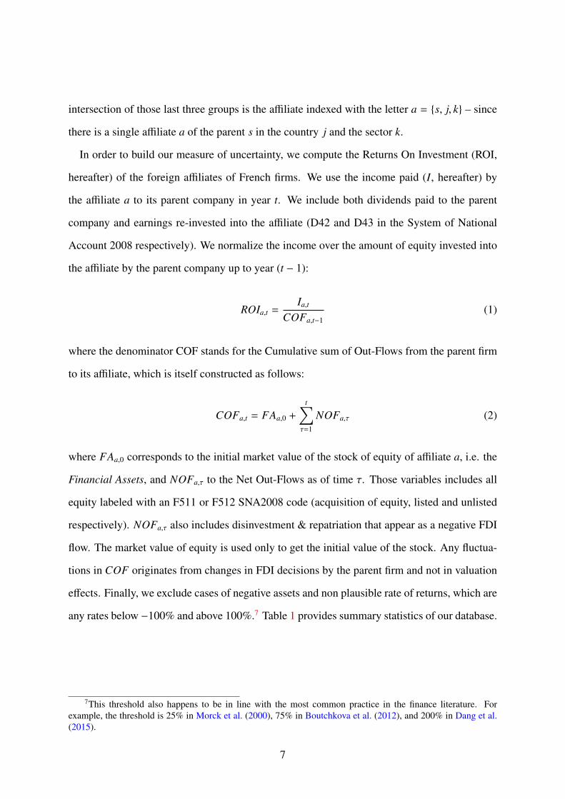
In order to build our measure of uncertainty, we compute the Returns On Investment (ROI,

hereafter) of the foreign affiliates of French firms. We use the income paid (I, hereafter) by

the affiliate a to its parent company in year t. We include both dividends paid to the parent

company and earnings re-invested into the affiliate (D42 and D43 in the System of National

Account 2008 respectively). We normalize the income over the amount of equity invested into

the affiliate by the parent company up to year (t − 1):

ROIa,t =Ia,t

COFa,t−1(1)

where the denominator COF stands for the Cumulative sum of Out-Flows from the parent firm

to its affiliate, which is itself constructed as follows:

COFa,t = FAa,0 +

t∑τ=1

NOFa,τ (2)

where FAa,0 corresponds to the initial market value of the stock of equity of affiliate a, i.e. the

Financial Assets, and NOFa,τ to the Net Out-Flows as of time τ. Those variables includes all

equity labeled with an F511 or F512 SNA2008 code (acquisition of equity, listed and unlisted

respectively). NOFa,τ also includes disinvestment & repatriation that appear as a negative FDI

flow. The market value of equity is used only to get the initial value of the stock. Any fluctua-

tions in COF originates from changes in FDI decisions by the parent firm and not in valuation

effects. Finally, we exclude cases of negative assets and non plausible rate of returns, which are

any rates below −100% and above 100%.7 Table 1 provides summary statistics of our database.

7This threshold also happens to be in line with the most common practice in the finance literature. Forexample, the threshold is 25% in Morck et al. (2000), 75% in Boutchkova et al. (2012), and 200% in Dang et al.(2015).

7

Table 1: Summary Statistics

N Mean P10 P50 P90 Std.Dev.Panel A Affiliate-levelAffiliate Assetsa,t (Mn.) 55021 180.47 0.90 15.65 254.98 1009.58Affiliate Flowsa,t (Mn.) 55021 8.30 -3.30 0.17 12.22 229.08ROIa,t (%) 55021 9.90 -8.94 5.23 39.81 24.66∆ COFa,t × 100 49869 3.37 -19.39 2.15 30.94 45.40Panel B Firm-levelAffiliates per firm 19387 2.97 1.00 2.00 7.00 3.43Parent Firm Assetss,k,t (Mn.) 19387 521.94 2.52 37.31 818.76 2567.50Parent Firm Flowss,k,t (Mn.) 19387 33.00 -5.34 0.66 46.61 426.55Panel C Country-levelAffilates per country 570 102.48 27.00 62.00 267.50 95.57French Assets j,t (Bn.) 570 17.89 0.72 3.92 50.73 33.19French Flows j,t (Bn.) 570 1.26 -0.01 0.29 3.04 3.54Panel D Year-levelAffilates per year 15 3894.27 2931.00 3782.00 4690.00 909.63French Assetst (Bn.) 15 679.83 430.22 688.85 957.81 210.41French Flowst (Bn.) 15 47.83 30.48 48.42 68.65 16.39

NOTE: Banque de France FDI databases, authors’ computation. Mn. indicates millions of Euros and Bn. billionsof euros.

2.3 Measuring Uncertainty on FDI Return

Our estimate of uncertainty is based on the following two-step procedure. The first step consists

in removing the forecastable component of the variation of affiliates’ returns. The forecasting

model of returns merge the portfolio approach of Boutchkova et al. (2012) for returns and the

methodology implemented by Bloom et al. (2018) for productivity. We break returns into a first

component explained by a set of regressors and a second unexplained component, the residuals,

as follows

ROIa,t = γ1ROIa,t−1 + γ2ROIt + γ3ROI j,t + γ j × γk + γs + ua,t (3)

where ROIa,t is the yearly return of affiliate a = {s, j, k} as of time t; γ j × γk capture time in-

variant country-sector specific heterogeneity while γs capture firm characteristics of the parent

company. The variables ROIt and ROI j,t are, respectively, the average world and country− j

8

returns of French MNF in period t. We compute them as follows:

ROIt =1At

At∑a∈t

ROIa,t, (4)

and

ROI j,t =1

A j,t

A j,t∑a∈ j

ROIa,t (5)

where At and A j,t are counters for the total number of affiliates in year t and country j in year t,

respectively.

We present the results of this first stage, equation (3), in Table 2. As expected, returns are

persistent (the coefficient of lagged returns is equal to 0.330 and significantly different form

zero) and highly correlated with the aggregate country and world returns. The systematic com-

ponent explains 28% of the variance of returns. We interpret the residuals as the idiosyncratic

returns (Boutchkova et al., 2012).

Table 2: 1st Stage Results

ROIa,t (%)ROIa,t−1 (%) 0.330∗∗∗

(0.00)Country average ROI 0.277∗∗∗

(0.00)World average ROI 0.252∗∗∗

(0.00)Constant 0.653

(0.34)Sector X Country FE YesParent Firm FE YesObservations 44018Adjusted R2 0.283p statistics in parentheses, with robust SE.∗ p < 0.10, ∗∗ p < 0.05, ∗∗∗ p < 0.01

In the second step, we calculate the country-specific moments of French affiliates idiosyn-

9

cratic returns as follows:

MEAN j,t =1

A j,t

A j,t∑a∈ j

ua,t (6)

where ua,t denotes the residuals from the estimation of equation (3), and

DISP j,t =

1A j,t − 1

×

A j,t∑a∈ j

(ua,t − MEAN j,t)2

1/2

(7)

where DISP j,t measures the dispersion of the residuals, e.g. how widely uninformative funda-

mentals are to predict firm specific returns. Throughout this paper, we will use DISP j,t as our

proxy for time varying uncertainty over the idiosyncratic returns of French MNF in country j.

In Section 4.1, we will extend our analysis to the third moment of the residual distributions,

namely the skewness, defined as follows

SKEW j,t =

1A j,t×

∑A j,t

a∈ j(ua,t − MEAN j,t)3[1

A j,t−1 ×∑A j,t

a∈ j(ua,t − MEAN j,t)2]3/2 (8)

The interest of the skewness is to consider asymmetric changes in risk as suggested by Ordonez

(2013), Orlik and Veldkamp (2014), Bloom et al. (2016), and Ruge-Murcia (2017) among

others – see Section 4.1 for more information.

2.4 Stylized Facts

The mean value of the uncertainty is 18.04 for the panel of 570 year-country observations, but

it varies substantially across time, countries, and sectors. Figure 1 shows the mean value of FDI

uncertainty for each year between 2001 and 2015. Uncertainty has declined from 2002 to 2007,

just before the financial crisis, and then increased between 2008 and 2009. Afterwards, it has

decreased once again to recover the pre-crisis level. This pattern is close to that of the VIX8,

but with notable differences (Figure A.1 in the appendix compares the two measures). Besides,

the interest of our measure of uncertainty is to vary across countries and sectors contrary to the

8The VIX is the implied volatility on the US stock market and is widely used as a worldwide measure ofuncertainty.

10

Figure 1: FDI Return Uncertainty

14

16

18

20

22

2000 2005 2010 2015

DISPt P25 P75

NOTE: This figure presents the yearly average, P25 and P75 of our measure of uncertaintyfor all countries, where the dispersion by country DISP j,t is defined by equation (7).

VIX index.

Dispersion across countries is quite large – the mean value of uncertainty by country is

reported in Table 3. It varies from 12.79 in Tunisia to 22.21 in Russia. Interestingly, the

dispersion does not seem related with the level of development. Uncertainty is high in some

emerging economies as Russia (but also in Romania or India), as we should expect, but very

low in Tunisia (but also in Thailand or South Korea). Actually, we do not find a significant cor-

relation between uncertainty and the real GDP per capita in our data. It is worth mentioning,

that we are not considering here the variance of realized returns but the variance of the idiosyn-

cratic component of returns after we control for country average returns and country(-sector)

fixed effects – see equation (3). Figure A.2 shows that the orthogonalization procedure was

successful. The second moment of the idiosyncratic performance shocks is less correlated with

country fundamental economic characteristics than the second moment of the raw returns. It

validates the use of DISP j,t as an exogenous source of uncertainty that we can causally identify.9

9Moreover, if we omit this procedure, the response function of FDI to the dispersion of the raw returns exhibitssome evidence of pre-trend issue.

11

Table 3: FDI Return Uncertainty

Affiliate-Year Return Uncertainty P25 P75ARG 664 18.44 13.07 24.71AUS 987 18.84 16.71 20.93AUT 591 18.19 14.56 21.34BEL 4050 16.15 13.92 18.04BRA 1602 19.00 16.41 21.41CAN 1450 16.34 14.23 17.91CHE 2302 18.72 16.83 20.59CHN 1573 19.18 17.45 20.27CIV 405 15.91 13.15 17.09CZE 959 19.17 15.53 24.67DEU 4109 19.17 17.63 19.85DNK 480 15.87 11.31 17.43ESP 4702 18.19 17.41 18.95FIN 303 17.07 13.08 21.67GBR 4316 17.02 15.26 18.08GRC 499 18.47 16.81 22.06HKG 852 19.55 17.88 21.86HUN 720 17.73 15.52 19.68IND 746 20.15 18.24 21.10IRL 699 18.37 16.03 20.47ITA 3725 19.61 17.07 21.81JPN 885 19.71 15.96 22.17KOR 628 14.17 12.25 15.70LUX 1404 15.08 13.65 16.05MAR 844 17.54 15.49 18.62MEX 780 17.41 13.93 20.51NLD 2744 16.93 14.77 18.21POL 1562 17.41 15.38 18.73PRT 1374 20.68 19.68 21.48ROU 555 21.11 18.08 22.62RUS 669 22.21 17.74 25.63SGP 918 19.88 17.34 22.96SWE 781 19.10 15.48 20.27THA 379 16.67 11.60 17.58TUN 447 12.79 9.56 15.23TUR 740 19.74 17.36 20.37USA 4104 17.07 15.58 18.07ZAF 473 17.91 13.68 20.19Total 55021 18.03 15.71 20.09

NOTE: Countries with at least 15 affiliates per year. Idiosyncratic Returns are based on the residualsfrom estimating Equation 3.

12

3 Impact of FDI Return Uncertainty on FDI Flows

This section investigates the effect of uncertainty on the direct investment activity of French

MNFs.

3.1 Baseline Regressions

Our baseline regression specification is as follows:

∆COFa,t = α1X j,t + α2Xs,t−1 + α3Xa,t−1 + β1DISP j,t + γa + γt × γk + εa,t (9)

where ∆COFa,t is the log difference of the cumulative stock of the affiliate a = {s, j, k} – owned

by the parent firm s in the sector k of the country j – as of time t.10 As in Julio and Yook

(2016) we use the log difference of the cumulative FDI position to avoid the issue of taking

the logarithm of negative flows. All the regressions include country level controls X j,t for GDP

growth, exchange rates changes, GDP per capita, trade openness and stock market return as in

Julio and Yook (2016) – see the section A.1 for data construction. We also include a vector

of lagged parent company controls Xs,t−1 to capture relevant firm characteristics for investment

(e.g. Gilchrist and Himmelberg (1995) and Gala and Julio (2016)): the log of the total direct

investment assets owned by the parent-firm to control for its size; the total number of foreign

affiliates owned by the parent-firm to proxy alternative investment opportunities; and finally

the parent-firm average return on investment to proxy the marginal return to capital. We add a

vector of lagged affiliate characteristics Xa,t−1 to control for its financial constraint and invest-

ment opportunities: the size of the affiliate assets and its returns on investment. Finally, we

follow Kovak et al. (2017) for the fixed effect structure: γa is an affiliate fixed effect that allows

us to control for affiliates unobservable time-invariant characteristics, including its country and

sector; γt × γk is a year by sector fixed effect that captures the business cycle of the sector.

The first column of Table 4 reports the estimation results of our baseline regression. The

10We cluster standard errors at the country level. Any other reasonable choice of clustering provides standarderrors of similar size.

13

Table 4: Idiosyncratic Uncertainty and FDI. Direct Effect and Effect Conditional on ParentCompany Past Performance

∆ COFa,t × 100

(1) (2) (3) (4)Performance

All Sample Low Medium Highlog GDP/cap. j,t 8.884∗∗∗ -9.197 27.485∗∗∗ 12.476∗∗∗

(2.837) (7.825) (5.623) (2.425)∆ GDP j,t 22.899 50.352 -12.642 13.954

(16.671) (40.692) (29.072) (14.216)∆ FX j,t -16.304∗∗∗ -10.533 -14.914∗ -24.066∗∗∗

(3.799) (8.309) (8.136) (5.504)Trade Openness j,t(%GDP) -0.039 -0.107∗∗ 0.006 0.003

(0.034) (0.049) (0.062) (0.036)Stock Market Return j,t -0.006 0.020 -0.042 0.007

(0.014) (0.031) (0.047) (0.030)log Parent Assetss,k,t−1 0.776 0.924 1.034 -0.630

(0.639) (1.290) (1.290) (1.026)Parent Performances,k,t−1 0.117∗∗ 0.429∗ 0.822∗ 0.192∗∗

(0.052) (0.239) (0.442) (0.079)Nb. of Foreign Affiliatess,k,t−1 -0.054 0.201 -0.029 -0.107

(0.138) (0.408) (0.369) (0.171)log Affiliate Assetsa,t−1 -6.359∗∗∗ -5.233∗∗∗ -5.912∗∗∗ -9.316∗∗∗

(0.651) (1.727) (1.143) (1.043)Affiliate Performancea,t−1 (%) 0.080∗∗∗ 0.018 0.080∗∗ 0.082∗∗∗

(0.026) (0.055) (0.037) (0.029)DISP j,t -0.213∗∗∗ -0.434∗∗ -0.243 -0.128

(0.073) (0.182) (0.154) (0.099)Affiliate FE Yes Yes Yes YesSector × Year FE Yes Yes Yes YesObservations 39499 10820 9266 17812R2 0.302 0.388 0.355 0.324Effect in pcp. of an IQR shift:- DISP j,t -0.904 -1.837 -1.026 -0.544- ∆ GDP j,t 0.582 1.234 -0.336 0.364

NOTES: We report standard errors clustered at the country level; * p < 0.10, ** p < 0.05, *** p < 0.01; a, s, k, jand t indexes affiliates, parent-firms, sectors, countries and years respectively.We estimate the results above on a sample of 3056 French parent companies and their 10474 foreign affilatesbetween 2001 and 2015 in 38 countries. See Section 2.3 for the construction of DISP j,t. The last two lines presentthe contrasts of shifting from the 25th percentile of the distribution of the selected variable to the 75th while holdingother variables constant at their mean value.

14

coefficient β1 of our variable of interest DISP j,t is negative, equal to −0.002, and significant at

the one percent level. The sign of the coefficient is consistent with the literature on the adverse

effects of uncertainty on investment. The magnitude of this estimated effect is substantial.

Indeed, shifting from the 25th percentile of the distribution of uncertainty to the 75th percentile

results in a 0.904 (s.e.= 0.412) points of percentage reduction in FDI growth rate – that is

approximately one quarter of the average growth rate of FDI in our data, namely 3.37%. As

a comparison, a similar shift in the distribution of GDP growth rate implies a 0.582 points of

percentage increase in FDI growth rate.11

When it comes to the control variables, as expected an increase in the GDP growth rate of

the destination country is associated with a higher flow of FDI to this country. The coefficient

for Trade Openness is negative but not significantly different from zero at the 10% level. De-

preciation of the local currency (that is a positive variation of the real FX rate) is associated

with lower FDI. The sign and significance of the coefficients for parent company and affiliate

characteristics provides an interesting complement to the results from Gala and Julio (2016):

the negative coefficient of the size of the affiliate reflects the diminishing returns of investment

opportunities rather than financial constraints. The positive but non statistically significant co-

efficient of the size of the parent company (after controlling for lagged returns) would indicate

that financial constraints do not play a major role in the FDI of multinational firms. The co-

efficients of other control variables for parent company (returns on investment and number of

affiliates) are not significantly different from zero.

We supplement our results with the Local Projection method of Jordà (2005)12 to assess the

persistence of the adverse effect of uncertainty on FDI. This is important with regards to the

rebound effect associated with the wait and see mechanism highlighted by Bernanke (1983)

and Bloom (2009). The initial negative effect should not be persistent and then turn positive,

11We have also tested the effect of the lagged values of uncertainty, that is using DISP j,t−1 instead of DISP j,t

in our benchmark regressions. Lagged uncertainty shocks have no significant effects on cross-border investment.This is consistent with the fact that our measure of uncertainty exhibit a very low degree of persistence. It can alsobe related with Julio and Yook (2016) who show that the effect of uncertainty on FDI occurs mainly within theelection years; years before elections are not associated with a fall in foreign investments.

12See Crouzet et al. (2017) and Favara and Imbs (2015) for recent applications of Local Projection method tomicro data.

15

reflecting the wait and see pattern documented by Julio and Yook (2016). We estimate the

following equation:

∆COFa,t+h = αh1X j,t + αh

2Xs,t−1 + αh3Xa,t−1 + βh

1DISP j,t + γha + γh

t × γhk + εa,t+h (10)

where h is the horizon of projection. Figure 2 shows the results. The sign of the coefficient

remains negative for up to two years and turns positive until the end of the five year window,

however it is not significantly different from zero at these horizons. Backward projections in

Figure 2 show the absence of a pre-trend. There is no ex-ante effect depending on the intensity

of the treatment.13

Figure 2: Affiliate Outcome Path Following an Interquartile Shift in the Distributionof Uncertainty

0.27

-0.07 -0.04

0.00

-0.90

-0.54

0.22

0.56

0.16

0.510.72

-2.0

-1.0

0.0

1.0

2.0

-4 -2 0 2 4 6Year

βh1DISPj,t

NOTE: This Figure presents estimates of βh1 (scaled up by a 100 times an Interquartile Range shift of

DISP j,t) from estimating this equation for h ∈ {−4, 6}: ∆COFa,t+h = αh1X j,t + αh

2Xs,t−1 + αh3Xa,t−1 +

βh1DISP j,t + γh

a + γht × γ

hk + εa,t. 95% error bands are displayed in gray with standard errors clustered at

the country level.

13The pre-trends also appear to be parallel for the various groups of size and performance. It will also be thecase in 3 and A.3, see below.

16

3.2 The role of firm ex-ante performances

Insights from the trade and uncertainty literature suggest that firms react heterogeneously to

increased volatility. To test whether the effect of uncertainty may be caused by a heteroge-

neous reactions across firm characteristics, we replicate our baseline regressions (9) and (10)

for split samples, i.e. the sub-samples of firms grouped according to their ex-ante characteris-

tics. Barrero et al. (2017) and Patnaik (2016) also use split-sample analyses to assess the effect

of uncertainty according to the level of firm leverage and to the degree of competition, respec-

tively.14 We focus here on the role of firm ex-ante performances and estimate the following

equation:

∆COFa,t+h =∑g∈Γ

(αh

1,gX j,t + αh2,gXs,t−1 + αh

3,gXa,t−1 + βh1,gDISP j,t

)1{a∈Γg

t }

+ γha + γh

t × γhk + εa,t+h

(11)

for h ∈ {−4, 6} period ahead. Where Γ are firms groups based on their ex-ante performance:

Γ(g=low)t = Γ

(P0,P40)t

Γ(g=medium)t = Γ

(P40,P60)t

Γ(g=high)t = Γ

(P60,P100)t

Columns (2)-(4) in Table 4 report the estimation results for h = 0 and Figure 3 presents the

estimates of the coefficient βh1 of Equation (11) for various horizon h.

For most control variables, coefficients share the same sign and level of significance for the

three groups of firms. When it comes to our main variable of interest, DISP j,t, the coefficient is

significant only for firms with ex-ante low performances and substantially higher than estimated

in average. Shifting from the 25th percentile of the distribution of uncertainty to the 75th

percentile results in a reduction of FDI growth rate twice higher for these firms when compared

14See Zwick and Mahon (2017) for a split sample analysis of the effect of taxes on investment according tofirm size.

17

with the full sample, e.g. a reduction of −3.38 of percentage points against −0.904.

Inspecting the dynamic responses in Figure 3 reveals a greater heterogeneity in the effects of

uncertainty shocks on firms. The negative impact of return uncertainty for firms in the bottom

40% of the distribution becomes even more dramatic four years after the shock with a reduction

of −3.94 percentage points in the FDI growth rate. Then, the impact becomes not significantly

negative for higher horizons. The effect of uncertainty shocks turns out to be positive for the

most performant firms (and significantly different from zero) two and three years after the

shocks with a peak of 2.60 percentage points. These heterogeneous effects produce a huge gap

of almost 6 points of percentage in FDI growth rate between most and less performing firms

three years after the shocks.15 Since we consider FDI growth rates, this transitory divergence

between firms results in permanent divergence in the stock of assets held abroad. We find that

most of the persistence is explained by the lack of recovery from the lower performing parent

firms. Lastly, it is interesting to observe that the wait-and-see pattern observed for the entire

sample of parent companies (e.g. the rebound effect) is actually driven by the heterogeneity of

firm reactions to uncertainty.

15We also test the coefficient of the interaction of DISP j,t and a dummy variable indicating that the firm belongsto the bottom 40 percent of past performance. We find that the slope of DISP j,t for the low performance group isnegative and statistically significant relative to the other group. The pattern of the response mostly matches thatof our key result in Figure 3 (bottom and top right panel).

18

Figure 3: Affiliate Outcome Path Following an Interquartile Shift in the Distributionof Uncertainty Conditional on Parent Company Past Performance

0.27 -0.07 -0.04 0.00-0.90 -0.54

0.22 0.56 0.16 0.51 0.72

-7.5

-5

-2.5

0

2.5

5

-4 -2 0 2 4 6Year

Uncertainty Shock

-0.33 -0.600.24 0.00

-1.84 -2.22-2.82

-3.38-3.94

-1.66

-0.07

-7.5

-5

-2.5

0

2.5

5

-4 -2 0 2 4 6Year

with Parent Performances,t-1 < P40

1.640.65 0.75

0.00-1.03 -1.45 -1.21 -0.78 -0.50

0.12-1.05

-7.5

-5

-2.5

0

2.5

5

-4 -2 0 2 4 6Year

with Parent Performances,t-1 ∈ [P40,P60]

-0.51 -0.34 -0.42 0.00-0.54

0.481.77

2.601.83 2.02

1.43

-7.5

-5

-2.5

0

2.5

5

-4 -2 0 2 4 6Year

with Parent Performances,t-1 > P60

NOTE: This Figure presents estimates of βh1,g (scaled up by a 100 times an Interquartile Range shift

of DISP j,t) from estimating this equation for h ∈ {−4, 6}: ∆COFa,t+h =∑

g∈Γ(αh1,gX j,t + αh

2,gXs,t−1 +

αh3,gXa,t−1 + βh

1,gDISP j,t)1{a∈Γgt }

+γha +γh

t ×γhk + εa,t. 95% error bands are displayed in gray with standard

errors clustered at the country level. The left panel includes the entire sample, The top left panelincludes the entire sample, the next three panels includes only the affiliates of parent companies whichwere, respectively, in the bottom 40%, middle 20% and top 40% of the performance distribution theyear before.

4 Robustness

We attempt various comparison and validation exercises.

4.1 Asymmetric Uncertainty

This section investigates the effects of asymmetric uncertainty. Our benchmark measure of

uncertainty is based on the second order moment of the distribution of shocks to FDI returns.

An increase in uncertainty is symmetric shift of the two sides of the distribution. We can

generalize our methodology to consider asymmetric shifts of the distribution in two different

19

ways.

First, we can consider higher moments of the distribution such as the skewness (the third

order moment). The interest of the skewness is to consider asymmetric changes in risk, while

our measure DISPi, j consists in symmetric changes for the two sides of the distribution. In-

deed, a fall in the skewness corresponds to a relative increase in the probability of extremely

bad realizations of shocks. By investigating the effects of skewness shocks on FDI, we con-

tribute to the growing literature on the skewness dynamics in business and financial cycles (e.g.

Ordonez, 2013; Orlik and Veldkamp, 2014; Bloom et al., 2016; Ruge-Murcia, 2017). Table 5

extends our baseline regression by including the SKEW j,t of the distribution as an explanatory

variable. In column (1), we introduce both DISP j,t and SKEW j,t as explanatory variables while in

column (2) only SKEW j,t is introduced. Our estimates of β1 is robust to the inclusion of SKEW j,t

as an additional control variables: the coefficient of DISP j,t (column 1 in Table 5) is slightly

lower when compared to that of reported in column (1) of Table 4, but still highly significantly

different from zero. Column (1) suggests that the magnitude of the impact of SKEW j,t on FDI is

stronger than that of DISP j,t. An interquartile range shift of the skewness generates a variation

of 1.645 points of percentage of the FDI growth rate. It is twice higher than the effect of a

similar shift of the dispersion, namely 0.844. This estimate of the impact of skewness shocks

is roughly unchanged when we drop DISP j,t from the regression – see column (2) in Table 5.

Figure 4 compares the dynamic effects of an decrease in SKEW j,t with that of an increase in

DISP j,t depicted in 3. An interquartile range shift of the skewness generates a stronger and

more persistent response of cross-border investments than a similar shift of the dispersion of

shocks.

The second way to consider asymmetric change in uncertainty is to split the sample of DISP j,t

into good and bad uncertainty as suggested by Bollerslev et al. (2017). We use the country-year

mean of the residuals ua,t to make the distinction between good and bad uncertainty. Country-

year dyads where the mean of the performance shocks is positive are assigned to the first group

and country-year dyads with negative performance shocks on average are assigned to the sec-

ond one.

20

Figure 4: Affiliate Outcome Path Following an Interquartile Shift in the Distributionof Skewness

-0.17

0.26

-0.09

0.00

-1.64

-1.36

-0.68

-0.29

-0.71

-0.54

-1.20

-3.0

-2.0

-1.0

0.0

1.0

-4 -2 0 2 4 6Year

DISPj,t (P25 to P75)SKEWj,t (P75 to P25)

NOTE: This Figure presents estimates of βh1 (scaled up by a 100 times an Interquartile Range shift of

DISP j,t) and βh2 (scaled up by a 100 times an Interquartile Range shift of SKEW j,t) from estimating those

equations for h ∈ {−4, 6}: ∆COFa,t+h = αh1X j,t + αh

2Xs,t−1 + αh3Xa,t−1 + βh

1DISP j,t + γha + γh

t × γhk + εa,t.

and ∆COFa,t+h = αh1X j,t + αh

2Xs,t−1 + αh3Xa,t−1 + βh

2SKEW j,t + γha + γh

t × γhk + εa,t. 95% error bands are

displayed in gray with standard errors clustered at the country level.

Results are reported in columns (3)-(4) of the Table 5. The coefficient associated with DISP j,t

(column 3) is negative. Its order of magnitude is less than half that of an increase in DISP j,t in

the full sample and it is not significantly different from zero. Meanwhile in the sub-sample of

countries with a positive mean, the effect is negative and much stronger. If we consider only

bad uncertainty, the effect of an interquartile range shift (-1.436) is close to be twice higher

than in our benchmark case (-0.904 in column 1 of Table 4).

Considering the skewness or the distinction between good and bad uncertainty highlights the

asymmetric impact of uncertainty: rising dispersion on the left side of the distribution (low

returns) is more painful than rising dispersion on the right side (high return). This conclusion

is consistent with the model developed in Section B based on the role of financial frictions.

21

Lenders are exposed to default risk in the event of low FDI returns. In the event of high

returns, this benefits the multinationals that receive the profits because the debt contract does

not index the interest on the profits made. Lenders therefore react logically more strongly to

an asymmetric increase in risk (biased towards low returns) than to a symmetric increase in

risk, with a stronger increase in the risk premium at the origin of a fall in credit demand and

cross-border investments by multinationals.

4.2 The role of firm size

This section investigates the role of firm size in shaping the effect of uncertainty on FDI. Size

and performance are generally correlated (at least in theory, e.g. Melitz and Ottaviano (2008))

but that is not the case in our sample. Indeed, the coefficient of correlation between Parent

Performance and Parent Size is around 0.06. Therefore, we investigate how firm size influences

the effect of uncertainty shocks. Results are reported in Figure A.3 replicate the Figure 3 using

regressions (11) for deciles of ex-ante size instead of ex-ante performances. Large firms are

not impacted by uncertainty shocks, whatever the horizons, while small firms are strongly and

lastingly affected.

4.3 Alternative uncertainty proxies

This section shows the effects of uncertainty shocks on FDI using alternative proxies for un-

certainty. Columns (1)-(4) of Table A.2 considers alternatively four alternative measure of

uncertainty: the volatility of the local stock market, the country measure of Economic Policy

Uncertainty, the Foreign Exchange rate return Volatility, and finally the average one-year ahead

forecast errors of the IMF.

The estimated coefficient is significantly different from zero only for foreign exchange rate

volatility. As explained by Jeanneret (2016) the sign of the relation between FX volatility

and FDI is actually both theoretically and empirically ambiguous. Interestingly, inspecting

the dynamic effects of FX uncertainty confirms the importance of firm heterogeneity. Figure

22

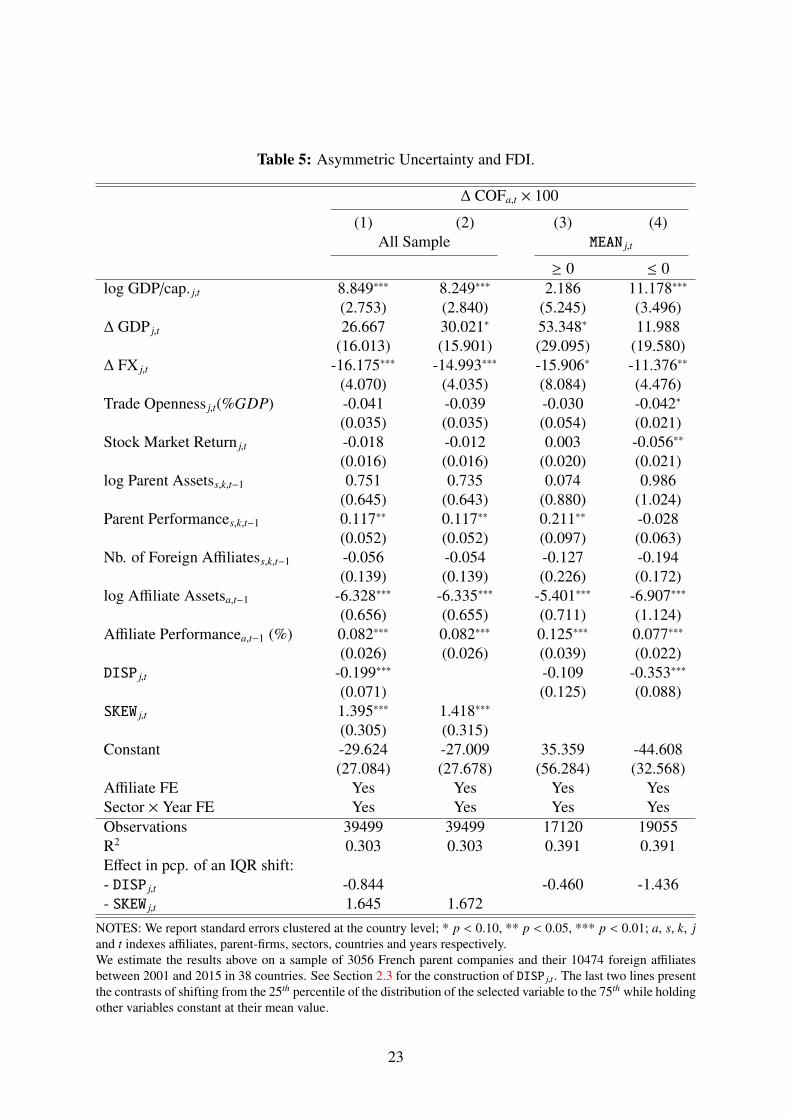
Table 5: Asymmetric Uncertainty and FDI.

∆ COFa,t × 100

(1) (2) (3) (4)All Sample MEAN j,t

≥ 0 ≤ 0log GDP/cap. j,t 8.849∗∗∗ 8.249∗∗∗ 2.186 11.178∗∗∗

(2.753) (2.840) (5.245) (3.496)∆ GDP j,t 26.667 30.021∗ 53.348∗ 11.988

(16.013) (15.901) (29.095) (19.580)∆ FX j,t -16.175∗∗∗ -14.993∗∗∗ -15.906∗ -11.376∗∗

(4.070) (4.035) (8.084) (4.476)Trade Openness j,t(%GDP) -0.041 -0.039 -0.030 -0.042∗

(0.035) (0.035) (0.054) (0.021)Stock Market Return j,t -0.018 -0.012 0.003 -0.056∗∗

(0.016) (0.016) (0.020) (0.021)log Parent Assetss,k,t−1 0.751 0.735 0.074 0.986

(0.645) (0.643) (0.880) (1.024)Parent Performances,k,t−1 0.117∗∗ 0.117∗∗ 0.211∗∗ -0.028

(0.052) (0.052) (0.097) (0.063)Nb. of Foreign Affiliatess,k,t−1 -0.056 -0.054 -0.127 -0.194

(0.139) (0.139) (0.226) (0.172)log Affiliate Assetsa,t−1 -6.328∗∗∗ -6.335∗∗∗ -5.401∗∗∗ -6.907∗∗∗

(0.656) (0.655) (0.711) (1.124)Affiliate Performancea,t−1 (%) 0.082∗∗∗ 0.082∗∗∗ 0.125∗∗∗ 0.077∗∗∗

(0.026) (0.026) (0.039) (0.022)DISP j,t -0.199∗∗∗ -0.109 -0.353∗∗∗

(0.071) (0.125) (0.088)SKEW j,t 1.395∗∗∗ 1.418∗∗∗

(0.305) (0.315)Constant -29.624 -27.009 35.359 -44.608

(27.084) (27.678) (56.284) (32.568)Affiliate FE Yes Yes Yes YesSector × Year FE Yes Yes Yes YesObservations 39499 39499 17120 19055R2 0.303 0.303 0.391 0.391Effect in pcp. of an IQR shift:- DISP j,t -0.844 -0.460 -1.436- SKEW j,t 1.645 1.672

NOTES: We report standard errors clustered at the country level; * p < 0.10, ** p < 0.05, *** p < 0.01; a, s, k, jand t indexes affiliates, parent-firms, sectors, countries and years respectively.We estimate the results above on a sample of 3056 French parent companies and their 10474 foreign affiliatesbetween 2001 and 2015 in 38 countries. See Section 2.3 for the construction of DISP j,t. The last two lines presentthe contrasts of shifting from the 25th percentile of the distribution of the selected variable to the 75th while holdingother variables constant at their mean value.

23

A.4 replicates the Figure 3 using regressions (11) with FX volatility instead of DISP j,t. As in

our benchmark, high performing firms react positively to an increase in uncertainty while low

performing firms experience an important and lastingly reduction in FDI. It is worth mention-

ing that this effect of exchange rate volatility on FDI does not affect that of the uncertainty

previously described. Indeed, the pattern depicted in Figure 2 is almost unchanged when the

exchange rate volatility is included among the control variables of equation (9).

Our results for stock price volatility are consistent with Gourio et al. (2016) who report

significant effects of uncertainty on total capital inflows who turn out to be non significant

when they consider only FDI inflows.16 We conclude that using micro-data allows us to build a

firm-level based measure of uncertainty which may be more relevant than aggregate measures

to capture its effects on firms decision.

4.4 Placebo Inference

In the baseline specification, we clustered standard errors at the country level. This provided us

with standard errors that are asymptotically robust to serial auto-correlation in the error term.

Here we implement Chetty et al. (2009)’s non-parametric permutation test17 of βh1 = 0.

To do so, we randomly reassign the uncertainty time serie across firms and then we re-

estimate the baseline regression. We repeat this process 2000 times in order to obtain an empir-

ical distribution of the placebo coefficients βh,p1 . If DISP j,t had no effect on FDI, we would ex-

pect our baseline estimate to fall somewhere in the middle of the distribution of the coefficients

of the placebo coefficients βh,p1 . Since that test does not rely on any parametric assumption re-

garding the structure of the error term, it is immune to the over-rejection of the null hypothesis

highlighted by Bertrand et al. (2004).

We plot the distribution of the placebo coefficients in Figure A.5. The figure confirms that our

coefficients of interest βh=01 (the blue connected markers) lie outside of the [p0.5,p99.5] interval

(the light blue lines) of the distribution of placebo coefficients. Meanwhile, the estimates of βh<01

16See the column 3 in Table 21 of Gourio et al. (2016)17See Malgouyres et al. (2019) for a more recent application

24

fall within the bounds of the distribution of placebos. This exercise confirms that uncertainty

has a negative effect on firm growth.

We repeat the same exercise for the other key finding of this paper. We randomly permute

DISP j,t within the sub-samples of low and high parent company ex-ante performance. Figure

A.6 confirms that each estimate of βh>01,g=low lies outside of its [0.5, 99.5] interval of its placebos

(the blue lines). Whereas the estimates of βh>01,g=high only fall outside of their intervals (in red) for

h = 3. Although this estimates are fairly close to the outside of the distribution of the placebos

for h = {1, 2, 4, 5}.

4.5 Specification Sensitivity

We show that the coefficient produced by our specification is not an outlier. We follow a

procedure somewhat similar to that of Campbell et al. (2019). We omit 1-by-1 each control

variable and plot the results in purple in Figure A.7. Then we test the following list of fixed

effects: s×m× jt; sm× jt; sm×t; s×m× j; m× jt; s jm×t; sm× jm×t; t.. All specifications include

the two following vectors of controls: X j,t = {GDP per capita, GDP growth, Exchange Rate

growth, Trade Openness, Market Return}; Xs,t−1 = {Size, Performance, Number of Affiliates}.

We plot the results in gold in Figure A.7. Our baseline specification falls in the middle of

the distribution of the coefficients. There is one outlying result for the specification that does

not include any time fixed-effect. Including the contemporaneous level of skewness and/or the

lagged value of uncertainty does not change our estimates.

4.6 Sample Sensitivity

Since our sample includes events such as the Great Financial Crisis (2008 and 2009), we wish

to check whether our results are robust to the omission of any particular year. We run the same

baseline regressions while omitting turn by turn any year between 2001 and 2015. Results are

quantitatively and qualitatively the same using these specifications as on the full sample; see

the thin blue lines in Figure A.8. This conclusion remains valid when the two years of the

25

Great Recession 2008-2009 are simultaneously dropped from the regression. Interestingly, it

turns out that the adverse effect of uncertainty on FDI is stronger when we consider only the

after-crisis period (2010-2015) than if one consider the pre-crisis period (2000-2007). It may

be interpreted as pervasive consequences of the Great Recession, even if we should remain

cautious given the slight difference in the values of the estimated coefficients for the two sub-

samples.

Finally, our estimate is also largely unchanged when taking out any sector (red lines) or

country (green lines) including the USA.

5 Conclusion

The main motivation of this study was to extract the information regarding uncertainty that

is embedded in FDI assets held abroad by french residents. We build a novel country and

time-varying proxy for uncertainty based on the idiosyncratic volatility of the returns of French

Foreign Direct Investment assets. Given this measure of uncertainty, we estimate how FDI

react to uncertainty by regressing the individual FDI outflows by French MNF on our measure

of uncertainty together with a set of relevant control variables and fixed effects.

An innovation in micro-uncertainty has a direct negative short-term impact on firm-level

flows to the affected country whereas commonly used proxy for risk/uncertainty fail to explain

most or any variation in flows. Following a one interquartile range increase in uncertainty in

one country, French MNF decrease the rate of their direct investments to the affected country

by as much as 0.904 (s.e.= 0.412) points of percentage. This effect decreases with the per-

formance of the parent firm. Using Local Projections, we show that on average, it has little

persistence beyond the initial shock. However, this effect hides strong parent-firm level hetero-

geneity. Indeed, parent companies with low ex-ante performance never recover while, higher

performing parent companies over compensate in the following periods.

Our empirical results suggest a cleansing effect of uncertainty shocks. The literature on

cleansing effect demonstrated that during recesssions less productive firms exit from the mar-

26

ket while the most productive survive (Caballero and Hammour, 1994; Foster et al., 2016;

Osotimehin and Pappadà, 2016; Aghion et al., 2019). We do not directly measure productivity

of firms in our database, but if we proxy it by the return of FDI, our results suggest a cleansing

effect too. Indeed, several years after an increase of uncertainty in a country, we should expect

a higher level of assets held by ex-ante high performing firms and a lower level of assets held by

ex-ante low performing firms. Interestingly, this reallocation process appears more important

between low and high performing firms than between small and large firms. Further researches

should be devoted to understand the mechanisms behind the heterogeneous behavior of firms

and the potential role of irreversibilities and financial constraints.

27

References

Aghion, P., A. Bergeaud, G. Cette, R. Lecat, and H. Maghin (2019). Coase

Lecture-the Inverted-U Relationship between Credit Access and Productivity Growth.

Economica 86(341), 1–31.

Aizenman, J. and N. Marion (2004). The merits of horizontal versus vertical FDI in the pres-

ence of uncertainty. Journal of International economics 62(1), 125–148.

Anderson, E. W., E. Ghysels, and J. L. Juergens (2009). The impact of risk and uncertainty on

expected returns. Journal of Financial Economics 94(2), 233–263.

Ang, A., R. J. Hodrick, Y. Xing, and X. Zhang (2006). The cross-section of volatility and

expected returns. The Journal of Finance 61(1), 259–299.

Ang, A., R. J. Hodrick, Y. Xing, and X. Zhang (2009). High idiosyncratic volatility and low

returns: International and further US evidence. Journal of Financial Economics 91(1), 1–23.

Atanassov, J., B. Julio, and T. Leng (2018). The bright side of political uncertainty: The case

of R&D.

Baker, S. R., N. Bloom, and S. J. Davis (2016). Measuring economic policy uncertainty. The

Quarterly Journal of Economics 131(4), 1593–1636.

Bar-Ilan, A. and W. C. Strange (1996). Investment lags. The American Economic

Review 86(3), 610–622.

Barrero, J. M., N. Bloom, and I. Wright (2017). Short and long run uncertainty. Technical

report, National Bureau of Economic Research.

Bernanke, B. S. (1983). Irreversibility, uncertainty, and cyclical investment. The Quarterly

Journal of Economics 98(1), 85–106.

Bernanke, B. S., M. Gertler, and S. Gilchrist (1999). The financial accelerator in

a quantitative business cycle framework. In J. B. Taylor and M. Woodford (Eds.),

28

Handbook of Macroeconomics, Volume 1 of Handbook of Macroeconomics, Chapter 21,

pp. 1341–1393. Elsevier.

Bertrand, M., E. Duflo, and S. Mullainathan (2004). How much should we trust differences-in-

differences estimates? The Quarterly journal of economics 119(1), 249–275.

Blanchard, O. and J. Acalin (2016). PB 16-17 What Does Measured FDI Actually Measure?

Bloom, N. (2009). The impact of uncertainty shocks. econometrica 77(3), 623–685.

Bloom, N. (2014). Fluctuations in uncertainty. The Journal of Economic Perspectives 28(2),

153–175.

Bloom, N., M. Floetotto, N. Jaimovich, I. Saporta-Eksten, and S. J. Terry (2018). Really

uncertain business cycles. Econometrica 86(3), 1031–1065.

Bloom, N., F. Guvenen, S. Salgado, et al. (2016). Skewed business cycles. In 2016 Meeting

Papers, Number 1621. Society for Economic Dynamics.

Bollerslev, T., S. Z. Li, and B. Zhao (2017). Good volatility, bad volatility, and the cross section

of stock returns. Journal of Financial and Quantitative Analysis, 1–57.

Boutchkova, M., H. Doshi, A. Durnev, and A. Molchanov (2012). Precarious politics and return

volatility. Review of Financial Studies 25(4), 1111–1154.

Caballero, R. J. and M. L. Hammour (1994). The cleansing effect of recessions. The American

Economic Review, 1350–1368.

Campbell, D., K. Mau, et al. (2019). Trade Induced Technological Change: Did Chinese

Competition Increase Innovation in Europe? Technical report.

Chetty, R., A. Looney, and K. Kroft (2009). Salience and taxation: Theory and evidence.

American economic review 99(4), 1145–77.

29

Christiano, L. J., R. Motto, and M. Rostagno (2014, January). Risk Shocks. American

Economic Review 104(1), 27–65.

Crouzet, N., N. R. Mehrotra, et al. (2017). Small and Large Firms Over the Business Cycle.

Technical report.

Cushman, D. (1985). Real Exchange Rate Risk, Expectations, and the Level of Direct Invest-

ment. The Review of Economics and Statistics 67(2), 297–308.

Dang, T. L., F. Moshirian, and B. Zhang (2015). Commonality in news around the world.

Journal of Financial Economics 116(1), 82–110.

De Sousa, J., A.-C. Disdier, and C. Gaigné (2018). Export decision under risk.

Dixit, A. (1992). Investment and hysteresis. The Journal of Economic Perspectives 6(1), 107–

132.

Favara, G. and J. Imbs (2015). Credit supply and the price of housing. American Economic

Review 105(3), 958–92.

Fernández-Arias, E. and R. Hausmann (2001). Foreign direct investment: Good cholesterol?

Inter-American Development Bank, Research Department Working Paper No 417.

Fillat, J. L. and S. Garetto (2015). Risk, returns, and multinational production. The Quarterly

Journal of Economics 130(4), 2027–2073.

Foster, L., C. Grim, and J. Haltiwanger (2016). Reallocation in the Great Recession: cleansing

or not? Journal of Labor Economics 34(S1), S293–S331.

Gala, V. and B. Julio (2016). Firm Size and Corporate Investment.

Ghosal, V. and P. Loungani (2000). The differential impact of uncertainty on investment in

small and large businesses. Review of Economics and Statistics 82(2), 338–343.

30

Gilchrist, S. and C. P. Himmelberg (1995). Evidence on the role of cash flow for investment.

Journal of Monetary Economics 36(3), 541–572.

Goldberg, L. and C. Kolstad (1995). Foreign Direct Investment, Exchange Rate Variability and

Demand Uncertainty. International Economic Review 36(4), 855–73.

Gourio, F., M. Siemer, and A. Verdelhan (2016). Uncertainty and International Capital Flows.

Guiso, L. and G. Parigi (1999). Investment and demand uncertainty. The Quarterly Journal of

Economics 114(1), 185–227.

Handley, K. and N. Limao (2015). Trade and investment under policy uncertainty: theory and

firm evidence. American Economic Journal: Economic Policy 7(4), 189–222.

Handley, K. and N. Limão (2017). Policy uncertainty, trade, and welfare: Theory and evidence

for china and the united states. American Economic Review 107(9), 2731–83.

Helpman, E., M. J. Melitz, and S. R. Yeaple (2004). Export versus fdi with heterogeneous

firms. American economic review 94(1), 300–316.

Héricourt, J. and C. Nedoncelle (2018). Multi-destination firms and the impact of exchange-

rate risk on trade. Journal of Comparative Economics.

Jeanneret, A. (2016, Aug). International Firm Investment under Exchange Rate Uncertainty.

Rev. Financ. 20(5), 2015–2048.

Jordà, Ò. (2005). Estimation and inference of impulse responses by local projections. American

Economic Review 95(1), 161–182.

Julio, B. and Y. Yook (2016). Policy uncertainty, irreversibility, and cross-border flows of

capital. Journal of International Economics 103, 13–26.

Jurado, K., S. C. Ludvigson, and S. Ng (2015). Measuring uncertainty. The American

Economic Review 105(3), 1177–1216.

31

Kovak, B. K., L. Oldenski, and N. Sly (2017). The labor market effects of offshoring by us

multinational firms: Evidence from changes in global tax policies. Technical report, National

Bureau of Economic Research.

Lewis, L. T. (2014). Exports versus multinational production under nominal uncertainty.

Journal of International Economics 94(2), 371–386.

Malgouyres, C., T. Mayer, and C. Mazet-Sonilhac (2019). Technology-induced Trade Shocks?

Evidence from Broadband Expansion in France. CEPR Discussion Papers 13847, C.E.P.R.

Discussion Papers.

Marmer, V. and M. E. Slade (2018). Investment and uncertainty with time to build: Evidence

from entry into us copper mining. Journal of Economic Dynamics and Control 95, 233–254.

Melitz, M. J. and G. I. Ottaviano (2008). Market size, trade, and productivity. The review of

economic studies 75(1), 295–316.

Mohn, K. and B. Misund (2009). Investment and uncertainty in the international oil and gas

industry. Energy Economics 31(2), 240–248.

Morck, R., B. Yeung, and W. Yu (2000). The information content of stock markets: why

do emerging markets have synchronous stock price movements? Journal of Financial

Economics 58(1), 215 – 260. Special Issue on International Corporate Governance.

Ordonez, G. (2013). The asymmetric effects of financial frictions. Journal of Political

Economy 121(5), 844–895.

Orlik, A. and L. Veldkamp (2014). Understanding uncertainty shocks and the role of black

swans. Technical report, National Bureau of Economic Research.

Osotimehin, S. and F. Pappadà (2016). Credit frictions and the cleansing effect of recessions.

The Economic Journal 127(602), 1153–1187.

Patnaik, R. (2016). Competition and the real effects of uncertainty.

32

Pindyck, R. S. (1991). Irreversibility, uncertainty, and investment. Journal of Economic

Literature 29(3), 1110–1148.

Ramondo, N., V. Rappoport, and K. J. Ruhl (2013). The proximity-concentration tradeoff under

uncertainty. Review of Economic Studies 80(4), 1582–1621.

Rodrik, D. (1991). Policy uncertainty and private investment in developing countries. Journal

of Development Economics 36(2), 229–242.

Ruge-Murcia, F. (2017). Skewness risk and bond prices. Journal of Applied

Econometrics 32(2), 379–400.

Russ, K. N. (2012). Exchange rate volatility and first-time entry by multinational firms. Review

of World Economics 148(2), 269–295.

Stein, L. C. and E. Stone (2013). The effect of uncertainty on investment, hiring, and r&d:

Causal evidence from equity options.

Townsend, R. M. (1979). Optimal contracts and competitive markets with costly state verifica-

tion. Journal of Economic Theory 21(2), 265–293.

Vicard, V. (2018). The exorbitant privilege of high tax countries. Working paper.

Zwick, E. and J. Mahon (2017, January). Tax policy and heterogeneous investment behavior.

American Economic Review 107(1), 217–48.

33

A Appendix

A.1 Data

Stock Price Volatility (SPV), GDP and GDP per capita are from the World Development In-

dicators (WDI) database from the World Bank. We obtain daily exchange rates against the

Euro from World Market Reuters to calculate their growth rate by taking the log difference

and then compute yearly average and volatility measures. The VIX is the implied volatility

index computed by the CBOE and EPU is the Economic Policy Uncertainty Index from Baker

et al. (2016). ∆GDP is computed by taking the log difference between year t and year t − 1.

Macro forecast errors are the dispersion of the IMF 1 year ahead forecast errors of GDP growth,

inflation and current account balance.

A.2 Additional Figures and Tables

Figure A.1: FDI Return Uncertainty and the VIX

10

15

20

25

30

35

17

18

19

20

21

2000 2005 2010 2015

DISPt VIX

Correlation: 0.558 N: 15

NOTE: Banque de France data and authors’ computations. The blue linepresents the mean yearly value of FDI return uncertainty and the red dashedline the mean yearly value of the VIX.

34

Figure A.2: Uncertainty and GDP/cap.

ARG

AUS

AUT

BEL

BRA

CAN

CHE

CHN

CIV

CZE

DEU

DNKESP

FIN

GBR

GRC

HKG

HUN

IND

IRL

ITAJPN

KOR

LUX

MAR

MEX

NLD

POL

PRT

ROU RUS

SGP

SWETHA

TUN

TUR

USA

ZAF

20

22

24

26

28

30

DIS

P j,t

7 8 9 10 11Log GDP/cap.

Correlation: -0.202 N: 38

ARGAUS

AUT

BEL

BRA

CAN

CHECHN

CIV

CZE DEU

DNK

ESP

FINGBR

GRC

HKG

HUN

IND

IRL

ITA JPN

KOR

LUX

MAR MEXNLD

POL

PRTROU

RUS

SGP

SWE

THA

TUN

TUR

USA

ZAF

12

14

16

18

20

22

DIS

P j,t

7 8 9 10 11Log GDP/cap.

Correlation: -0.036 N: 38

NOTE: Banque de France data and authors’ computations. The figure shows the relation-ship between the period average value of log GDP per capita and the dispersion of the rawFDI returns (left panel) and the dispersion of the idiosyncratic returns (right panel).

35

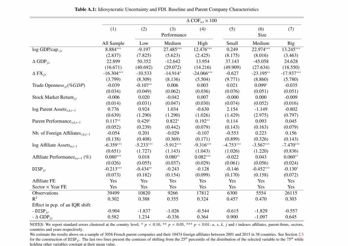
Table A.1: Idiosyncratic Uncertainty and FDI. Baseline and Parent Company Characteristics

∆ COFa,t × 100

(1) (2) (3) (4) (5) (6) (7)Performance Size

All Sample Low Medium High Small Medium Biglog GDP/cap. j,t 8.884∗∗∗ -9.197 27.485∗∗∗ 12.476∗∗∗ 0.249 22.974∗∗∗ 13.245∗∗∗

(2.837) (7.825) (5.623) (2.425) (8.175) (8.016) (3.463)∆ GDP j,t 22.899 50.352 -12.642 13.954 37.143 -45.058 24.628

(16.671) (40.692) (29.072) (14.216) (49.909) (27.634) (18.550)∆ FX j,t -16.304∗∗∗ -10.533 -14.914∗ -24.066∗∗∗ -0.627 -23.195∗∗ -17.937∗∗∗

(3.799) (8.309) (8.136) (5.504) (9.771) (8.860) (5.780)Trade Openness j,t(%GDP) -0.039 -0.107∗∗ 0.006 0.003 0.021 0.099∗ -0.035

(0.034) (0.049) (0.062) (0.036) (0.076) (0.051) (0.051)Stock Market Return j,t -0.006 0.020 -0.042 0.007 -0.000 0.000 -0.009

(0.014) (0.031) (0.047) (0.030) (0.074) (0.052) (0.016)log Parent Assetss,k,t−1 0.776 0.924 1.034 -0.630 2.154 -1.149 -0.802

(0.639) (1.290) (1.290) (1.026) (1.429) (2.975) (0.797)Parent Performances,k,t−1 0.117∗∗ 0.429∗ 0.822∗ 0.192∗∗ 0.114 0.093 0.045

(0.052) (0.239) (0.442) (0.079) (0.143) (0.163) (0.079)Nb. of Foreign Affiliatess,k,t−1 -0.054 0.201 -0.029 -0.107 -0.553 0.223 0.156

(0.138) (0.408) (0.369) (0.171) (0.899) (0.326) (0.143)log Affiliate Assetsa,t−1 -6.359∗∗∗ -5.233∗∗∗ -5.912∗∗∗ -9.316∗∗∗ -4.753∗∗∗ -3.567∗∗∗ -7.470∗∗∗

(0.651) (1.727) (1.143) (1.043) (1.026) (1.220) (0.836)Affiliate Performancea,t−1 (%) 0.080∗∗∗ 0.018 0.080∗∗ 0.082∗∗∗ -0.022 0.043 0.060∗∗

(0.026) (0.055) (0.037) (0.029) (0.061) (0.056) (0.024)DISP j,t -0.213∗∗∗ -0.434∗∗ -0.243 -0.128 -0.146 -0.452∗∗∗ -0.130∗

(0.073) (0.182) (0.154) (0.099) (0.170) (0.158) (0.072)Affiliate FE Yes Yes Yes Yes Yes Yes YesSector × Year FE Yes Yes Yes Yes Yes Yes YesObservations 39499 10820 9266 17812 6300 5554 26115R2 0.302 0.388 0.355 0.324 0.457 0.470 0.303Effect in pcp. of an IQR shift:- DISP j,t -0.904 -1.837 -1.026 -0.544 -0.615 -1.829 -0.557- ∆ GDP j,t 0.582 1.234 -0.336 0.364 0.900 -1.097 0.645

NOTES: We report standard errors clustered at the country level; * p < 0.10, ** p < 0.05, *** p < 0.01; a, s, k, j and t indexes affiliates, parent-firms, sectors,countries and years respectively.We estimate the results above on a sample of 3056 French parent companies and their 10474 foreign affiliates between 2001 and 2015 in 38 countries. See Section 2.3for the construction of DISP j,t. The last two lines present the contrasts of shifting from the 25th percentile of the distribution of the selected variable to the 75th whileholding other variables constant at their mean value.

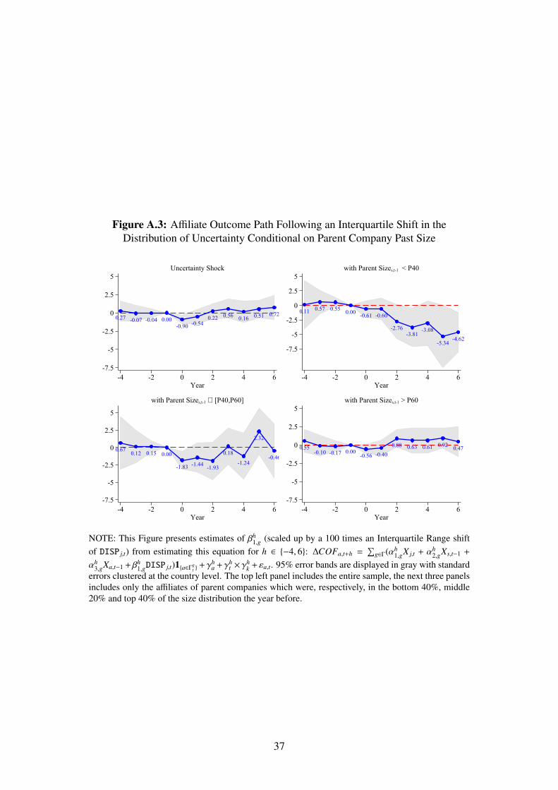
Figure A.3: Affiliate Outcome Path Following an Interquartile Shift in theDistribution of Uncertainty Conditional on Parent Company Past Size

0.27 -0.07 -0.04 0.00-0.90 -0.54

0.22 0.56 0.16 0.51 0.72

-7.5

-5

-2.5

0

2.5

5

-4 -2 0 2 4 6Year

Uncertainty Shock

0.11 0.57 0.55 0.00 -0.61 -0.60

-2.76-3.81

-3.08

-5.34-4.62

-7.5

-5

-2.5

0

2.5

5

-4 -2 0 2 4 6Year

with Parent Sizes,t-1 < P40

0.67 0.12 0.15 0.00

-1.83 -1.44 -1.93

0.18

-1.24

2.32

-0.46

-7.5

-5

-2.5

0

2.5

5

-4 -2 0 2 4 6Year

with Parent Sizes,t-1 ∈ [P40,P60]

0.55-0.10 -0.17 0.00

-0.56 -0.400.88 0.63 0.61 0.92 0.47

-7.5

-5

-2.5

0

2.5

5

-4 -2 0 2 4 6Year

with Parent Sizes,t-1 > P60

NOTE: This Figure presents estimates of βh1,g (scaled up by a 100 times an Interquartile Range shift

of DISP j,t) from estimating this equation for h ∈ {−4, 6}: ∆COFa,t+h =∑

g∈Γ(αh1,gX j,t + αh

2,gXs,t−1 +

αh3,gXa,t−1 + βh

1,gDISP j,t)1{a∈Γgt }

+γha +γh

t ×γhk + εa,t. 95% error bands are displayed in gray with standard

errors clustered at the country level. The top left panel includes the entire sample, the next three panelsincludes only the affiliates of parent companies which were, respectively, in the bottom 40%, middle20% and top 40% of the size distribution the year before.

37

Table A.2: Standard Risk Proxy and FDI

∆ COFa,t × 100

(1) (2) (3) (4)log GDP/cap. j,t 15.351∗∗∗ 6.410∗ 11.982∗∗∗ 14.725∗∗∗

(3.411) (3.224) (3.044) (3.177)∆ GDP j,t 51.780∗∗ 59.689∗∗ 48.891∗∗ 47.178∗

(22.501) (25.583) (18.680) (24.421)∆ FX j,t -14.623∗∗∗ -13.948∗∗ -14.471∗∗∗ -15.025∗∗∗

(5.070) (5.554) (4.393) (4.904)Trade Openness j,t(%GDP) -0.021 -0.118 -0.048 -0.020

(0.032) (0.080) (0.037) (0.033)Stock Market Return j,t 0.008 -0.004 -0.008 0.007

(0.024) (0.024) (0.017) (0.024)log Parent Assetss,k,t−1 1.740∗∗ 2.750∗∗∗ 1.724∗∗ 1.750∗∗

(0.753) (0.685) (0.695) (0.748)Parent Performances,k,t−1 0.197∗∗∗ 0.132∗∗ 0.200∗∗∗ 0.199∗∗∗

(0.050) (0.054) (0.048) (0.049)Nb. of Foreign Affiliatess,k,t−1 0.012 -0.115 -0.064 0.001

(0.166) (0.159) (0.140) (0.163)log Affiliate Assetsa,t−1 -10.128∗∗∗ -10.233∗∗∗ -9.964∗∗∗ -10.137∗∗∗

(0.989) (1.385) (0.942) (0.991)Affiliate Performancea,t−1 (%) -0.003 0.024 0.008 -0.005

(0.031) (0.040) (0.027) (0.031)Stock Price Volatility j,t 0.043

(0.076)Econ. Policy Unc. j,t 0.010

(0.011)Foreign Exchange Volatility j,t 68.785∗∗

(32.235)Macro FC ERR j,t -0.045

(0.209)Affiliate FE Yes Yes Yes YesSector × Year FE Yes Yes Yes YesObservations 36068 24121 39754 36085R2 0.298 0.304 0.290 0.298Effect in pcp. of an IQR shift:- Variable of Interest 46.99 54.16 168.9 -5.950- ∆ GDP j,t 138.9 145.3 126.8 126.7

NOTES: We report standard errors clustered at the country level; * p < 0.10, ** p < 0.05, *** p < 0.01; s, k, jand t indexes firms, sectors, countries and years respectively.We estimate the results above on a sample of 3056 French parent companies and their 10474 foreign affilatesbetween 2001 and 2015 in 38 countries. See Section 2.3 for the construction of DISP j,t. The last two lines presentthe contrasts of shifting from the 25th percentile of the distribution of the selected variable to the 75th while holdingother variables constant at their mean value.

38

Figure A.4: Affiliate Outcome Path Following an Interquartile Shift in theDistribution of Foreign Exchange Rate Volatility Conditional on Parent Company

Past Performance

0.16 -0.21 0.37 0.001.94

0.38

-2.74 -3.31-1.99 -1.21

2.45

-10

-5

0

5

10

-4 -2 0 2 4 6Year

FXV Shock

2.32

7.69

2.230.00

2.13 1.08

-3.76-7.25

-11.24

-16.92

-7.27

-30

-20

-10

0

10

-4 -2 0 2 4 6Year

with Parent Performances,t-1 < P40

-0.71 -2.040.95 0.00 1.63 0.15

2.04 2.29

-2.70

3.470.90

-20

-10

0

10

20

-4 -2 0 2 4 6Year

with Parent Performances,t-1 ∈ [P40,P60]

1.32

-1.47-0.35 0.00

2.82 2.37

-1.160.33

2.41

5.096.84

-5

0

5

10

15

-4 -2 0 2 4 6Year

with Parent Performances,t-1 > P60

NOTE: This Figure presents estimates of βh1,g (scaled up by a 100 times an Interquartile Range shift

of FXV j,t) from estimating this equation for h ∈ {−4, 6}: ∆COFa,t+h =∑

g∈Γ(αh1,gX j,t + αh

2,gXs,t−1 +

αh3,gXa,t−1 + βh

1,gFXV j,t)1{a∈Γgt }

+ γha + γh

t × γhk + εa,t. 95% error bands are displayed in gray with standard

errors clustered at the country level. The top left panel includes the entire sample, the next three panelsincludes only the affiliates of parent companies which were, respectively, in the bottom 40%, middle20% and top 40% of the performance distribution the year before.

39

Figure A.5: Placebo Test: Whole Sample for all horizons

-2

-1

0

1

2

-4 -2 0 2 4 6

NOTE: This Figure presents each semi-percentile of the distribution of 2000estimates of the coefficients βh

1 of our variable of interest DISP j,t (scaled up bya 100 times an Interquartile Range shift of DISP j,t) after performing a randompermutation. The sequence of coefficients of our main result is displayed in darkblue.

Figure A.6: Placebo Test: Low Perf. vs High Perf. for allhorizons

-4.0

-2.0

0.0

2.0

4.0

-4 -2 0 2 4 6

Low Perf. High Perf.

NOTE: This Figure presents each semi-percentile of the distribution of 2000estimates of the coefficients βh

1,g of our variable of interest DISP j,t (scaled upby a 100 times an Interquartile Range shift of DISP j,t) after performing a ran-dom permutation within each sub-sample. Results for low performing firms aredisplayed in blue and high performing firms in red.

40

Figure A.7: Specification Sensitivity

-1.0

0.0

1.0

2.0

3.0

-4 -2 0 2 4 6

Baseline Control Var.Fixed Effects incl. DISPj,t-1

incl. SKEWj,t

NOTE: The figure presents estimate of our coefficient of interest β1 (scaled upby a 100 times an Interquartile Range shift of DISP j,t) for various combinationsof controls.

Figure A.8: Sample Sensitivity

-1.0

-0.5

0.0

0.5

1.0

-4 -2 0 2 4 6

Baseline CountrySector Year

NOTE: This figure presents the distribution of the estimates of our coefficientof interest β1 (scaled up by a 100 times an Interquartile Range shift of DISP j,t)while removing turn by turn any cluster of observations in our sample (2-digitsectors in red, countries in green, years in blue).

41

Table A.3: Other Summary Statistics

Panel A Country-level N Mean Median Std.Dev.Stock Price Volatility j,t 514 22.55 21.00 9.22Econ. Policy Unc. j,t 220 117.21 111.63 43.56Foreign Exchange Volatility j,t 570 0.02 0.02 0.02Macro FC ERR j,t 529 2.31 1.91 1.92∆ GDP j,t 570 0.03 0.03 0.03∆ FX j,t 570 0.02 0.00 0.09Trade Openness j,t(%GDP) 570 99.48 73.52 84.31GDP per capita j,t 570 29658 27694 23122Panel B GlobalAffilates per year 15 3894.27 3782.00 909.63French Assetst (Bn.) 15 679.83 688.85 210.41French Flowst (Bn.) 15 47.83 48.42 16.39

Stock Price Volatility (SPV), GDP and GDP per capita are from the WorldDevelopment Indicators (WDI) database from the World Bank. We obtaindaily exchange rates against the Euro from World Market Reuters and use itto compute yearly average and volatility measures. The VIX is the impliedvolatility index computed by the CBOE and EPU is the Economic Policy Un-certainty Index from Baker et al. (2016).

42

B Theoretical Explanation

This section provides an illustrative model to explain the effect of uncertainty shocks on foreign

investments and accounting for heterogeneous responses of multinational firms. The model

is based on the costly-state verification setup originally developed by Townsend (1979) and

therefore incorporates in dynamic general equilibrium model by Bernanke et al. (1999). We

follow the extension of this model by Christiano et al. (2014) who make uncertainty time-

varying as the outcome of "Risk shocks". More precisely, we extend the partial and static

equilibrium developed by Christiano et al. (2014) in their Appendix D to solve the market

equilibrium for assets traded between domestic shareholders and multinational firms.

B.1 Assumptions

The model solves the partial market equilibrium for assets of domestic firms supplied by local

shareholders to foreign investors. The supply of assets is decreasing with respect to the return

yields, paid by local shareholders to foreign investors, according to

As = A − η × ROI (1)

where A > 0 is the inelastic supply of assets and η > 0 the elasticity of asset supply with respect

to return yields, denoted ROI as in our empirical setup.

The demand for assets is the outcome of the maximization of expected returns by a con-

tinuum of multinational firms, which size is equal to one. To buy assets, they combine own

capital, denoted N, and debt borrowed to financial intermediaries, denoted B. Then, the de-

mand for assets Ad by the representative firm satisfies the financing constraint

Ad = N + B (2)

In this static and partial equilibrium, capital N is treated as exogenous. The amount of debt

B and the debt interest rate Z are however endogenous and determined by the optimal debt

43

contract in the context of costly-state verification. Indeed, the multinational firm is exposed

to an idiosyncratic shock on its return denoted ω. Idiosyncratic return shocks are distributed

according to a lognormal distribution F (ω) which mean is equal to one, Eω = 1, and the

standard deviation of log (ω) is σ. After realization of the shock, the return on assets isω×ROI.

There is a threshold ω such that the multinational firm is unable to reimburse the debt if return

shock ω is below this value: ω ≤ ω. The threshold value ω satisfies

(1 + ROI)ωAd = (1 + Z) B (3)

and can be expressed as follows

ω =1 + Z

1 + ROIBAd =

1 + Z1 + ROI

L − 1L

(4)

where L = Ad/N is the leverage ratio. The threshold ω and the default rate F (ω) are both

increasing with the leverage ratio L and the ratio of debt interest rate to asset returns (1 +

Z)/(1 + ROI). Taking into account the default risk, expected returns are

∫ ∞ω

[(1 + ROI)ωAd − (1 + Z) B

]dF (ω)

N (1 + R)(5)

where R the risk-free interest rate accounts for the opportunity costs of investing capital N in

assets instead of risk-free assets. Multinational firm earn profits only if they draw a return

shock ω above the default threshold ω, otherwise the financial intermediary seize all assets and

revenues.

The participation constraint of the financial intermediary to the contract writes as follows

[1 − F (ω)

](1 + Z) B + (1 − µ)

∫ ω

0ω (1 + ROI) AddF (ω) = (1 + R) B (6)

With a probability[1 − F (ω)

], the borrower does not default and reimburses debt and interests

(1 + Z) B. In the case of default, the financial intermediary seizes the revenues from assets,

44

namelyω (1 + ROI) Ad, but incurs monitoring costs which represent a share µ of these revenues.

Financial intermediaries borrow at the risk-free interest rate R.

It is useful hereafter to consider the notation introduced by Bernanke et al. (1999) for Γ (ω) =

ω[1 − F (ω)

]+G (ω;σ) which determines the sharing rule of revenues and G (ω) =

∫ ω

0ωdF (ω)

which is the average return of defaulting entrepreneurs. The entrepreneurs receive the share[1 − Γ (ω)

]of revenues while the financial intermediary gets only

[Γ (ω) − µG (ω)

]since she

supports the monitoring costs µ.

B.2 Equilibrium

The optimal debt contract is the set of variables {ω,Z, B} that maximizes the entrepreneur ex-

pected returns (5) subject to the participation constraint of financial intermediary (6) and the

definition of the idiosyncratic return threshold (3).The equilibrium value of the threshold value

ω solves1 − F (ω)1 − Γ (ω)

=

[1 − F (ω) − µωF′ (ω;σ)

] 1+ROI1+R

1 −[Γ (ω) − µG (ω)

] 1+ROI1+R

(7)

Then, the amount of debt B is deduced from (6) and can be expressed as follows

L =1

1 −[Γ (ω) − µG (ω)

] 1+ROI1+R

(8)

Finally, (4) gives the loan interest rate Z

1 + Z = ω (1 + ROI)L

L − 1(9)

The definition of the equilibrium is as follows.

Definition 1. The equilibrium is the set of variables{ω,Z, B,ROI, As, Ad

}which satisfies: the

financial contract equilibrium equations: (7), (8), and (9); the supply of assets form the local

shareholders (1) and the demand of assets by multinational firms (2); the market equilibrium for

assets As = Ad; given the risk-free rate R, the capital of multinational firms N, the monitoring

45

cost µ, the elasticity η and exogenous component A of the supply function of assets, the level of

uncertainty σ, and the definition of the functions F (·) , Γ (·), and G (·).

B.3 Numerical simulations

We are interested in the impact of an increase in σ on the equilibrium. Unfortunately, it is not

feasible to characterize analytically the effects on σ, then we use numerical simulations.

The monitoring costs and the level of uncertainty are taken from Christiano et al. (2014)

(Appendix D): µ = 0.21 and σ = 0.26. Then, the risk-free is set to 2%, R = 0.02, and we

impose a return of 2% for assets taken from for our data, ROI = 0.09. Then, the following

variables are deduced: the default risk is slightly above 10% (F = 0.10) and the leverage ratio

more than three (L = 3.59). The supply elasticity of assets is set to one (η = 1), as the capital

of multinational firms (N = 1), and we deduce A = 4.66.

Figure B.9 shows the effect of increasing uncertainty σ in this model. Since multinational

firm draw more extremely low values of idiosyncratic return shocks, there are more defaults

in the economy as illustrated by the increase in F. Then, financial intermediaries ask for a

higher interest rate Z to cover the higher monitoring costs and firms decrease their demand for

debt and therefore their demand for domestic firm assets. As a results, the total investment

in the domestic market for assets A decreases and the yield on these assets ROI increases as

a compensation of the higher risk supported. Without considering fixed costs and extensive

margin, but financial frictions, this model can therefore explain the negative average effect

of uncertainty on FDI described in our empirical results. Can this model also explain the

heterogeneity of the effects between multinational firms?

To investigate the effect of heterogeneity in this model, we assume that multinational firm

differ with respect to the monitoring costs µ which takes now two values µ and µ, with µ >

µ. The population of firm, still normalized to the unity, is divided into two sub-populations

of equal size. All firms have the same amount of wealth. Figure B.10 shows the effect of

increasing uncertainty σ in this model. As in the case with homogeneous firms, there is an

46

0.22 0.24 0.26 0.28 0.3

0.08

0.09

0.1

0.11

0.12

0.13

0.14Default Risk: F

0.22 0.24 0.26 0.28 0.31.02

1.025

1.03

1.035

1.04

1.045Credit Premium: (1+Z)/(1+R)

0.22 0.24 0.26 0.28 0.31.055

1.06

1.065

1.07

1.075

1.08Return: (1+ROI)/(1+R)

0.22 0.24 0.26 0.28 0.33.58

3.585

3.59

3.595

3.6

3.605Investment: A

Figure B.9: Financial contract and market equilibrium for assets

47

0.22 0.24 0.26 0.28 0.30.04

0.06

0.08

0.1

0.12

0.14Default Risk: F

0.22 0.24 0.26 0.28 0.31.01

1.015

1.02

1.025

1.03

1.035

1.04

1.045Credit Premium: (1+Z)/(1+R)

0.22 0.24 0.26 0.28 0.31.055

1.06

1.065

1.07

1.075

1.08Return: (1+ROI)/(1+R)

0.22 0.24 0.26 0.28 0.31.7

1.8

1.9

2

2.1

2.2Investment: A

low µhigh µ

low µhigh µ

low µhigh µ

Figure B.10: Financial contract and market equilibrium for assets with heterogeneousmultinational firms

increase in the default risk and in the risk premium for all firms and the fall in demand for

domestic assets leads to an increase in the yields. The new fact is that we observe a divergence

in investment. Firms with high monitoring costs decrease their investment while firms with

low monitoring costs increase their investment. Firms with higher monitoring costs are more

concern by the increase in uncertainty, since default is more costly for them, and therefore react

more strongly than firms with low monitoring costs who get back market shares. Consistently

with our empirical results the model describes a reallocation process of market shares between

firms after an increase in uncertainty.

48