critical-path planning and scheduling - mosaic projects

160 1959 PROCEEDINGS OF THE EASTERN JOINT COMPUTER CONFERENCE

Critical-Path Planning and Scheduling

JAMES E. KELLEY, JR.t AND MORGAN R. W ALKERt

INTRODUCTION AND SUMMARY

JMONG the major problems facing technical management today are those involving the coordination of many diverse activities toward a common

goal. In a large engineering project, for example, almost all the engineering and craft skills are involved as well as the functions represented by research, development, design, procurement, construction, vendors, fabricators and the customer. Management must devise plans which will tell with as much accuracy as possible how the efforts of the people representing these functions should be directed toward. the project's completion. In order to devise such plans and implement them, management must be able to collect pertinent information to accomplish the following tasks:

(1) To form a basis for prediction and planning

(2) To evaluate alternative plans for accomplishing the objective

(3) To check progress against current plans and objectives, and

(4) To form a basis for obtaining the facts so that decisions can be made and the job can be done.

Many present project planning systems possess deficiencies resulting from techniques inadequate for dealing with complex projects. Generally, the several groups concerned with the work do their own detailed planning and scheduling - largely independent from one another. These separate efforts lead to lack of coordination. Further, it is traditional in project work that detailed schedules be developed frbm gross estimates of total requirements and achievements based on past experience. The main reason for this oversimplification stems from the inability of unaided human beings to cope with sheer complexity. In consequence, many undesirable effects may arise. Some important aspects of a project, which should be taken into account at the outset, may be ignored or unrecognized. As a result, much confusion may arise during the course of the project. When this happens, the management of the project is left to the coordinators and expediters. In such circumstances, management loses much of the control of a project and is never quite sure whether its objectives are being attained properly.

Reconizing the deficiencies in traditional proJect planning and scheduling procedures, the Inte-

t Mauchly Associates, Inc., Ambler, Pa.

grated Engineering Control Group (I. E. C.) of E. I. duPont de Nemours & Co. proceeded to explore possible alternatives. It was felt that a high degree of coordination could be obtained if the planning and scheduling information of all project functions are combined into a single master plan - a plan that integrates all efforts toward a common objective. The plan should point directly to the difficult and significant activities - the problems of achieving the objective. For example, the plan should form the basis of a system for management by exception. That is, within the framework of the rules laid down, it should indicate the exceptions. Under such a system, management need act only when deviations from the plan occur.

The generation of such a coordinated master plan requires the consideration of much more detailed information at one time than heretofore contemplated in project work. In turn, a new approach to the whole problem of planning and scheduling large projects is required. In late 1956, I. E. C. initiated a survey of the prospects for applying electronic computers as an aid to coping with the complexities of managing engineering projects. The following were the questions of most pressing interest: To what extent can a computer-oriented system be used:

(1) To prepare a master schedule for a project?

(2) To revise schedules to meet changing conditions in the "most" economical way?

(3) To keep management and the operating departments advised of project progress and changes?

During the course of this survey outside help was solicited. As part of their customer service, Remington Rand UNIVAC assigned the first author to the job of providing some assistance. At the time the second author represented duPont in this effort. The result of our alliance is the subject of this essay.

We made a critical analysis of the traditional approach to planning and a study of the nature of engineering projects. It quickly became apparent that if a new approach were to be successful, some technique had to be used to describe the interrelationships among the many tasks that compose a project. Further, the technique would have to be very simple and rigorous in application, if humans were to cope with the complexity of a project.

One of the difficulties in the traditional approach is that planning and scheduling are carried on simultaneously. At one session, the planner and scheduler

From the collection of the Computer History Museum (www.computerhistory.org)

Kelly and Walker: Critical-Path Planning and- Scheduling 161

consider - or attempt to consider - hundreds of details of technology, sequence, duration times, calendar deliveries and completions, and cost. With the planning and scheduling functions broken down in a step by step manner, fruitless mental juggling might be avoided and full advantage taken of the available information.

Accordingly, the first step in building a model of a project planning and scheduling system was to separate the functions of planning from scheduling. We defined planning as the act of stating what activities must occur in a project and in what order these activities must take place. Only technology and sequence were considered. Scheduling followed planning and is defined as the act of producing project timetables in consideration of the plan and costs.

The next step was to formulate an abstract model of an engineering project. The basic elements of a project are activities or jobs: determination of specs, blueprint preparation, pouring foundations, erecting steel, etc. These activities are represented graphically in the form of an arrow diagram which permits the user to study the technological relations among them.

Cost and execution times are associated with each activity in the project. These factors are combined with the technological relations to produce optimal direct cost schedules possessing varying completion dates. As a result, management comes into possession of a spectrum of possible schedules, each having an engineered sequence, a known elapsed time span, a known cost function, and a calendar fit. In the case of R&D projects, one obtains "most probable" schedules. From these schedules, management may select a schedule which maximizes return on investment or some other objective criterion.

The technique that has been developed for doing this planning and scheduling is called the CriticalPath Method. This name was selected because of the central position that critical activities in a project play in the method. The Critical-Path Method is a general interest from several aspects:

(1) It may be usea to solve a class of "practical" business problems

(2) It requires the use of modern mathematics

(3) Large-scale computing equipment is required for its full implementation

(4) It has been programmed for three computersUNIVAC I, 1103A and 1105 with a Census Bureau configuration

(5) It has been put into practice

In what follows we will attempt to amplify these points. We will describe various aspects of the mathematical model first. The mathematics involved will be treated rather superficially, a detailed development being reserved for a separate paper. The second part of this essay will cover the experience and

results obtained from the use of the Critical-Path Method.

PART I: ANALYSIS OF A PROJECT

1. Project Structure

Fundamental to the Critical-Path Method is the basic representation of a project. It is characteristic of all projects that all work must be performed in some well-defined order. For example, in construction work, forms must be built before concrete can be poured; in R&D work and product planning, specs must be determined before drawings can be made; in advertising, artwork must be made before layouts can be done, etc.

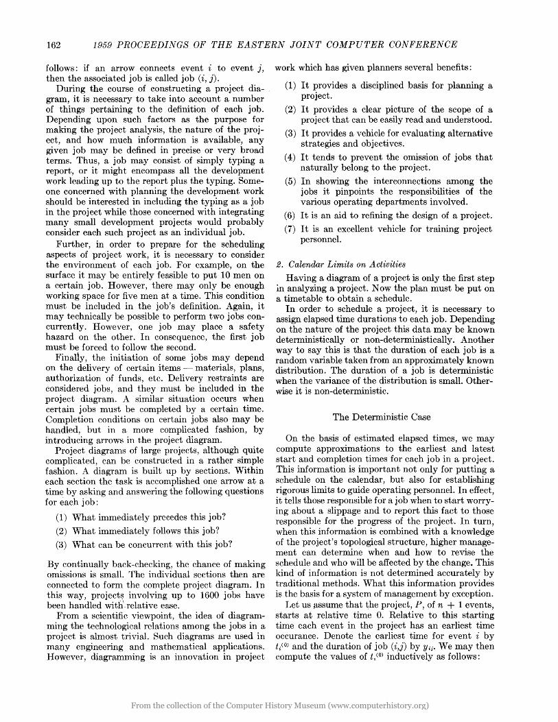
These relations of order can be shown graphically. Each job in the project is represented by an arrow which depicts (1) the existence of the job, and (2) the direction of time-flows from the tail to the head of the arrow). The arrows then are interconnected to show graphically the sequence in which the jobs in the project must be performed. The result is a topological representation of a project. Fig. 1 typifies the graphical form of a project.

1 .' 7

Fig. 1-Typical project diagram.

Several things should be noted. It is tacitly assumed that each job in a project is defined so that it is fully completed before any of its successors can begin. This is always possible to do. The junctions where arrows meet are called events. These are points in time when certain jobs are completed and others must begin. In particular there are two distinguished events, origin and terminus, respectively, with the property that origin precedes and terminus follows every event in the project.

Associated with each event, as a label, is a nonnegative integer. It is always possible to label events such that the event at the head of an arrow always has a larger label than the event at the tail. We assume that events are always labeled in this fashion. For a project, P, of n + 1 events, origin is given the label 0 and terminus is given the label n.

The event labels are used to designate jobs as



follows: if an arrow connects event i to event j, then the associated job is called job (i, j).

During the course of constructing a project dia- . gram, it is necessary to take into account a number of things pertaining to the definition of each job. Depending upon such factors as the purpose for making the project analysis, the nature of the project, and how much information is available, any given job may be defined in precise or very broad terms. Thus, a job may consist of simply typing a report, or it might encompass all the development work leading up to the report plus the typing. Someone concerned with planning the development work should be interested in including the typing as a job in the project while those concerned with integrating many small development projects would probably consider each such proje~t as an individual job.

Further, in order to prepare for the scheduling aspects of project work, it is necessary to consider the environment of each job. For example, on the surface it may be entirely feasible to put 10 men on a certain job. However, there may only be enough working space for five men at a time. This condition must be included in the job's definition. Again, it ITlay technically be possible to perform two jobs concurrently. However, one job may place a safety hazard on the other. In consequence, the first job must be forced to follow the second.

Finally, the initiation of some jobs may depend on the delivery of certain items - materials, plans, authorization of funds, etc. Delivery restraints are considered jobs, and they must be included in the project diagram. A similar situation occurs when certain jobs must be completed by a certain time. Completion conditions on certain jobs also may be handled, but in a more complicated fashion, by introducing arrows in the project diagram.

Project diagrams of large projects, although quite complicated, can be constructed in a rather simple fashion. A diagram is built up by sections. Within each section the task is accomplished one arrow at a time by asking and answering the following questions for each job:

(1) What immediately precedes this job?

(2) What immediately follows this job?

(3) What can be concurrent with this job?

By continually back-checking, the chance of making omissions is small. The individual sections then are connected to form the complete project diagram. In this way, project~ involving up to 1600 jobs have been handled with'. relative ease.

From a scientific viewpoint, the idea of diagramming the technological relations among the jobs in a project is almost trivial. Such diagrams are used in many engineering and mathematical applications. However, diagramming is an innovation in project

work which has given planners several benefits:

(1) It provides a disciplined basis for planning a project.

(2) It provides a clear picture of the scope of a project that can be easily read and understood.

(3) It provides a vehicle for evaluating alternative strategies and objectives.

(4) It tends to prevent the omission of jobs that naturally belong to the project.

(5) In showing the interconnections among the jobs it pinpoints the responsibilities of the various operating departments involved.

(6) It is an aid to refining the design of a project.

(7) It is an excellent vehicle for training project personnel.

2. Calendar Limits on Activities

Having a diagram of a project is only the first step in analyzing a project. Now the plan must be put on a timetable to obtain a schedule.

In order to schedule a project, it is necessary to assign elapsed time durations to each job. Depending on the nature of the project this data may be known deterministically or non-deterministically. Another way to say this is that the duration of each job is a random variable taken from an approximately known distribution. The duration of a job is deterministic when the variance of the distribution is small. Otherwise it is non-deterministic.

The Deterministic Case

On the basis of estimated elapsed times, we may compute approximations to the earliest and latest start and completion times for each job in a project. This information is important not only for putting a schedule on the calendar, but also for establishing rigorous limits to guide operating personnel. In effect, it tells those responsible for a job when to start worrying about a slippage and to report this fact to those responsible far the progress of the project. In turn, when this information is combined with a knowledge of the project's topological structure, higher management can determine when and how to revise the schedule and who will be affected by the change. This kind of information is not determined accurately by traditional methods. What this information provides is the basis for a system of management by exception.

Let us ~,ssume that ~he project, P, of n + 1 events, starts at relative time o. Relative to this starting tirne each event in the project has an earliest time occurance. Denote the earliest time for event i by t/O) and the duration of job (i,j) by Yij. We may then compute the values of t~(O) inductively as follows:


Kelly and Walker: Critical-Path Planning and Scheduling 163

(1) {to(O) = 0 t/O) = max [Yt} +t/O) Ii <j, (i,j)E P], 1 ~j ~n.

Similarly, we may compute the latest time at which each event in the project may occur relative to a fixed project completion time. Denote the latest time for event i by tP). If A is the project completion time (where A ~ tn(O») we obtain

(2)

Having the earliest and latest event times we may compute the following important quantities for each job, (i, j), in the project:

Earliest start time Earliest completion time = ti(O) - Ytj Latest start time = t}O) - Yi l

Latest completion time = t/O)

Maximum time available = tp) - tt(O) If the maximum ti~e available for a job equals its

duration the job is called critical. A delay in a critical job will cause a comparable delay in the project completion time. A project will contain critical jobs only when A = tn (0). If a project does contain critical jobs, then it also contains at least one contiguous path of critical jobs through the project diagram from origin to terminus. Such a path is called a critical-path.

If the maximum time available for a job exceeds its duration, the job is called a floater. Some floaters can be displaced in time or delayed to a certain extent without interfering with other jobs or the completion of the project. Others, if displaced, will start a chain reaction of displacements downstream in the project.

It is desirable to know, in advance, the character of any floater. There are several measures of float of interest in this connection .. The following measures are easily interpreted:

Total Float = t/ 1) - tt(O) - Ytj Free Float = t/O) - tt (0) - Y i}

Independent Float = max (0, t}(O) - tt(l) - Yij) Interfering Float = t} (1) - t} (0).

N on-Deterministic Schedules Information analogous to that obtained in the

deterministic case is certainly desirable for the nondeterministic case. It would be useful for scheduling applied research directed toward a well-defined objective.

However, in attempting to develop such information some difficulties are encountered which do not seem easily resolved. These difficulties are partly philosophical and partly mathematical. Involved is the problem of defining a "meaningful" measure for the criticalness of a job that can be computed in a "reasonable" fashion.

Although a complete analysis of this situation is

not germane to the development of the Critical-Path Method, it is appropriate, however, to indicate some concepts basic to such an analysis. Thus, in the nondeterministic case we assume that the duration y .. , '1)

of activity (i, j) is a random variable with probability density Gij(y). As a consequence it is clear that the time at which an event occurs is also a random variable, t}, with probability density H}(t). We assume that event 0 is certain to ocCUr at time O. Further on the assumption that it is started as soon as possible, we see that ti + Y ti = Xih the completion time for job (i, j), is a random variable with probability density Si}(X):l

(3)

jG,,~x), if i ~ 0

-l £ H,(u)G;;(x - u) du, (i, j)E P.

Assuming now that an event occurs at the time of the completion of the last activity preceding it we can easily compute the probability density, Hi(t), of

ti = max [Xii I (i, j)E P, i < j] ,

where Xij is taken from S ij(X) :

Several methods are available for approximating SiieX) and R}(t). The one which suits our taste is to express Gtj(y) in the form of a histogram with equal class intervals. The functions Sij(X) and Hj(t) are then histograms also and are computed in the obvious way by replacing integrals by sums. It would seem that in practice one can afford to have fairly large class intervals so that the chore of computing is qui te reasonable. .

In computing Sij(X) and Hi(t) above we assumed that job (i,j) was JStarted at the time of the occurrance of t i • For various reasons it may not be desirable to abide by this assumption. Indeed, it may be possible to delay the start of job (i, j) to a fair extent after the actual occurance of ti without changing the character of H}(t). However, the assumption we have made does provide a probabilistic lower bound on the start time Jor job (i, j). By analogy with the deterministic case we may think of Hi(t) as the probability density of the earliest start time for job (i, j). Similarly, Sij(X) in (3) then becomes the probability density of the earliest completion time for job (i, j). In this sense, (4) ·is the probabilistic analogue of (1).

I t is desirable to be able to measure the criticalness of each job in the project. Intuitively one is tempted to use the probabilistic analogue of (2), running the project backward from some fixed or r,andom comple-

lSee M. G. Kendall, "The Advanced Theory of Statistics,'~ Vol. 1, J. B. Lippincott Co., 1943, p. 247.



tion time as was done in the deterministic case. In this way one might hope to obtain information about the latest time at which events can occur, so that probabilistic measures of float might be obtained. It appears that this is a false hope since, among other things, such a procedure assumes that the project start time is a random variable and not a certain event. (The project start time can always be assumed certain, simply by making lead time for the project start on the day the calculations are made.)

To proceed further we must introduce the notion of "risk" in defining the criticalness of a job. On the basis of this definition one would hope to obtain probabilistic measures for float which would be useful for setting up a system for management by exception. We will not explore these possibilities further here.

3. The project cost function

In the deterministic case, the durations of jobs may sometimes be allowed to vary within certain limits. This variation may be attributed to a number of factors. The elapsed-time duration of a job may change as the number of men put on it changes, as the type of equipment or method used changes, as the work week changes from 5 to 6 to 7 days, etc. Thus, management has considerable freedom to choose the elapsed-time duration of a job, within certain limitations on available resources and the technology and environment of the job. Every set of job durations selected will lead to a different schedule and, in consequence, a different project duration. Conversely, there are generally many ways to select jQb durations so that the resulting schedules have the same shortest time duration.

Faced with making a choice, management must have some way of evaluating the merits of each possibility. In traditional planning and scheduling systems such a criterion is not too well defined. In the present context, however, there are several possibilities. The one we will focus our attention upon is cost.

Job Cost

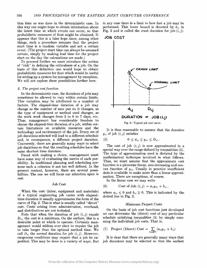
When the cost (labor, equipment and materials) of a typical engineering job varies with elapsedtime duration it usually approximates the form of the curve of Fig. 2. This is what is usually called "direct" cost. Costs arising from administration, overhead, and distributives are not included.

Note that when the duration of job (i, j) equals Dih the cost is a minimum. On the surface, this is a desirable point at which to operate. Certainly management would seldom ever elect to require the job to take longer than the optimal method time. We call Dii the normal duration for job (i, j). However, exogenous conditions may require that a job be expedited. This may be done in a variety of ways. But

in any case there is a limit to how fast a job may be performed. This lower bound is denoted by dti in Fig. 2 and is called the crash duration for job (i, j).

JOB COST

LIMIT

d'J Di.j

DURATION Of' JOB (itJ)

Fig. 2-Typical job cost curve.

It is thus reasonable to assume that the duration YiJ of job (i, j) satisfies

(5)

The cost of job (i, J) is now approximated in a special way over the range defined by inequalities (5). The type of approximation used is dictated by the mathematical technique involved in what follows. Thus, we must assume that the approximate cost function is a piecewise linear, non-increasing and convex function of Y ii. Usually in practice insufficient data is available to make more than a linear approximation. There are exceptions, of course.

In the linear case we may write

(6) Cost of Job (i, j) = aiiYii + b iJ ,

where aii ~ 0 and b ii ~ O. This is indicated by the dotted line in Fig. 2.

Minimum Project Costs

On the basis of job cost functions just developed we can determine the (direct) cost of any particular schedule satisfying inequalities (5) by simply summing the individual job costs. That is,

(7) Project (Direct) Cost = L (aiiYii + b ii) (i,j,EP)

It is clear that there are generally many ways that job durations may be selected so that the earliest



completion times of the resulting schedules are all equal. However, each schedule will yield a different value of (7), the project cost. Assuming that all conditions of the project are satisfied by these schedules, the one which costs the least invariably would be selected for implementation.

It is therefore desirable to have a means of selecting the least costly schedu1e for any given feasible earliest project completion time. Within the framework we have already constructed, such "optimal" schedules are obtained by solving the following linear program: Minimize (7) subject to (5) and

(8) Yij ~ tj - t i , (i, j)E P , and (9) to = 0, tn = A •

Inequalities (8) express the fact that the duration of a job cannot exceed the time available for performing it. Equations (9) require the project to start at relative time 0 and be completed by relative time A. Because of the form of the individual job cost functions, within the limits of most interest, A is also the earliest project completion time.

At this point it should be noted that the case where each job cost function is non-increasing, piecewise linear and convex is also reducible to a parametric linear program (see [7] and [8]). It does not add anything essential here to consider this more generalized form.

A convenient tool for generating schedules for various values of A is the method of parametric linear programming with A as the parameter. Intuitively, this technique works as follows. Initially, we let Yij = Dij for every job in the project. This is called the all-normal solution. We then assume that each job is started as early as possible. As a result we can compute tt (0) for all events. In particular, the earliest project completion time for this schedule is A = tn (0) •

By the nature of the job cost functions this schedule is also a minimum cost schedule for A = tn (0) • We now force a reduction in the project completion time by expediting certain of the critical jobs - those jobs that control project completion time. Not all critical jobs are expedited, but only those that drive the project cost up at a minimum rate as the project completion time decreases. As the project completion is reduced, more and more jobs become critical and thus there is a change in which jobs are to be expedited. This process is repeated until no further reduction in project completion time is possible.

Mathematically speaking, the process utilizes a primal-dual algorithm (see [6]). The restricted dual problem is a network flow problem involving both positive upper and lower bound capacity restrictions. A form of the Ford-Fulkerson network flow algorithm [3] is used to solve it. The critical jobs that are expedited at each stage of the process correspond to a cut set in the graph of all critical jobs.

PRO~E.CT DIRECT COST

{

CHARACTERISTIC

r MINIMUM COST SCJ.lEDUL.ES

PROJECT DUR.ATION - A Fig. 3-Typical project cost curve.

This process produces a spectrum of schedules (characteristic solutions in the linear programming sense) each at minimum total (direct) cost for its particular duration. When the costs of these schedules are plotted versus their respective durations, we obtain a non-increasing, piecewise linear, convex function as depicted in Fig. 3. This function is called the proj'ect cost curve.

Uses of the Project Cost Curve

The project cost curve only reflects the direct costs (manpower, equipment and materials) involved in executing a project. However, other costs are involved which contribute to the total project cost, such as overhead and administrative costs and perhaps even penalties for not completing a project or some portion of it by a certain time. These external costs must be taken into account when management plans how the project should be implemented relative to overall objectives.

Relative to these external costs there are at least two types of considerations that management may make:

(1) The (direct) cost curve for the project may be compared with the indirect cost of overhead and administration to find a schedule which minimizes the investment cost.

(2) The investment cost curve may be compared with market losses, as when it is desired to meet the demands of a rising market in a competitive situation. The schedule selected in this case is one which maximizes return on investment.



4. Manpower Leveling

As developed in this paper, the Critical-Path Method is based primarily on the technological requirements of a project. Considerations of available manpower and equipment are conspicuous by their absence. All schedules computed by the technique are technologically feasible but not necessarily practical. For example, the equipment and manpower requirements for a particular schedule may exceed those available or may fluctuate violently with time. A means of handling these difficulties must therefore be sought - a method which "levels" these requirements.

Here we will outline the approach we have taken to this problem. We restrict the discussion to manpower, similar considerations being applicable to leveling equipment requirements.

The term "manpower leveling" does not necessarily mean that the same number of men should be used throughout the project. It usually means that no more men than are available should be used. Further, if this requirement is met, one should not use the maximum number of men available at one instant in time and very few the very next instant of time.

The difficult part of treating the manpower leveling problem from a mathematical point of view is the lack of any explicit criteria with which the "best" use of manpower can be obtained. Under critical examination, available levels of manpower and also changes in level are established arbitrarily. This situation exists to some degree regardless of the organization involved. Even in the construction industry, where the work is by nature temporary, the construction organization desires the reputation of being a consistent "project life" employer. The organization wants the employee to feel that once "hired on" he can be reasonably sure of several months' work at the very least. In plants and in technical and professional engineering fields the same situation exists but with more severity. The employee is more acutely aware of "security", and the employer much more keenly aware of the tangible costs of recruitment and layoff as well as the intangible costs of layoff to his overall reputation and well-being.

In most organizations idle crafts and engineers or the need for new hires are treated with overwhelming management scrutiny. This is an excellent attitude, but too often this consideration is short range and does not consider long range requirements.

The following approaches to this problem have been made:

Incorporating Manpower Sequences

It is possible to incorporate manpower availability in the project diagram. However, this approach can cause considerable difficulty in stating the diagram

and may lead to erroneous results. Therefore, we recommend that this approach be dropped from consideration.

For example, assume there are three jobs - A, B, and C - that, from a technological viewpoint, can occur concurrently. However, each job requires the same crew. We might avoid the possibility that they occur simultaneously by requiring that A be followed by B, followed by C. It is also possible to state five other combinations - ACB, BCA, BAC, CAB, and CBA.

If we assume that this example occurs many times in a large arrow diagram, then there is not one, but a very large number of possible diagrams that can be drawn.

Now suppose a manpower sequence was not incorporated in the diagram and schedules were computed. It could be that the float times available for jobs A, B, and C are sufficient to perform the jobs in any of the six possible time sequences. However, by incorporating manpower sequences, we would never really know the true scheduling possibilities.

Examining Implied Requirements

Currently this method is performed manually and has been successfully used by applications personnel. It is possible to do much of the work involved by computer but, thus far, computer programs have not been prepared.

In preparing the work sheets for each activity, a statement is made of how many men per unit of time by craft are required for each duration. The planning and scheduling then proceeds in the manner prescribed by the Critical-Path Method. After a schedule is selected from all of the computed schedules, work on manpower leveling starts.

The first task is to tabulate the force required to execute the jobs along the critical path. Manpower commitments must be made to do these jobs at specific calendar dates. If manpower is not available, a longer duration schedule must be selected and the force requirements re-evaulated.

If adequate manpower is available to perform the critical jobs, then the total work force required by time units is tabulated. This is done by assuming every job starts at its earliest start date. The tabulation also is done, except assuming that every job starts at its latest start date.

Two total force curves result. These are then examined to be sure that they conform with some implicit statement of desired force. If not, the floaters are displaced to smooth the force curve. (In practice it has been found that one should displace the jobs with the least float first.)

During the tabulation and leveling processes, subtotals are kept by craft to ensure that, even though total force may be all right, craft restrictions also are met.



The smoothing (a purely heuristic process) is done until the desired force and craft curves are obtained, or until it is discovered that the schedule requires an unavailable force. In this case, the next longer schedule is selected, and the process is repeated until satisfactory results are obtained.

In one actual case, it was determined after attempts at smoothing that 27 mechanics were required when only 8 were available. Smoothing for this condition meant about a 20% lengthening of the critical path. Armed with this information, the planning and scheduling staff placed in management's hands a quantitative measure of the meaning of a manpower shortage so that, in advance, corrective action could be taken.

Solving for Best Fit

A procedure has been developed for computer programming that again is subjective in approach. One does not "solve" for the "best" force on the basis of some objective criteria. Rather, one states in advance what is "best" and then attempts to find ·the "best" fit.

The procedure is similar to examining the implied force requirements.

The total force curve desired, and craft breakdowns if requir~d, constitute the input. Then a stepby-step procedure is followed to move the floaters so that the resultant force curve approximates the desired force curve. If the results are unsatisfactory, the procedure would be to begin again with a schedule of longer duration.

The detailed method is too long for presentation here. In its present form, it is too involved for manual use except on very small projects. The logical steps are not too difficult, but for even modest-size projects the amount of storage required for "keeping track of" program steps dictates a fairly large computer for economical processing.

5. An Accounting Basis for Project Work

From the very start of the development of the Critical-Path Method, it has been the practice to assign a cost account number or job work order number to every job in a project. With this data, a structure can be set up for accruing costs against the proper accounts as the project proceeds.

Because each job in a project has a cost curve associated with it, as duration times are computed, it is a simple matter to compute the estimated individual job cost for a schedule. This computation gives management and supervision the basis for project cost control. As actual costs are incurred they can be compared with estimated costs and analyzed for exceptions. Time and cost control are in herent in the system.

One of the difficult tasks on certain types of project work is closing the project to capital investment

accounts. This frequently is not completed until long after the project ends. There are several reasons for the delay. One is that costs are sometimes not accrued so that they may easily be identified and/or apportioned to the proper facility. Another is the sheer magnitude of the accounting job. Under the Critical-Path system, it is possible to do this job as you go, keeping current with the project. Just as it is easy to close a project, it is easy to estimate in advance capital expenditures for labor, equipment and materials. This can mean many dollars in savings to project management in efficient capital usage.

PART II: HISTORICAL DEVELOPMENT

AND RESULTS

1. Early Developments

The fundamentals of the system outlined in Part I were developed during early 1957. Preliminary results were reported in [4] and [5]. By May 1957 the theory had advanced to the point where it was felt that the approach would be successful. At that time a cooperative effort to implelnent the method was undertaken by Remington Rand and duPont in order to determine the extent to which any further work was advisable. Remington Rand supplied the required programs for duPont's UNIVAC I located in Newark, Delaware. Engineers from duPont provided a small pilot problem with which to make the preliminary tests.

The results of this phase of the development were officially demonstrated in September, 1957. The demonstration showed that the technique held great promise. Accordingly, further tests of the system were authorized. These tests were set up to determine several things, among which were the following major points:

(1) To see if the data required were available and, if not, how difficult they would be to obtain

(2) To see if an inlpartial group of engineers could be trained to use the new method

(3) To see if the output from the new scheduling system was competitive in accuracy and utility with the traditional method

(4) To determine what kind of computing equipment is required for this type of application

(5) To see if the new system was economical.

2. Selecting a Team

By late December 1957 a team of six engineers was formed, and work on the test was under way. The team consisted of a field superintendent, a division engineer, and two area engineers, all with experience from construction, a process engineer from design, and an estimator. It is important to note tha t all these men had some experience in each of the other's specialty. For this reason they had very



little difficulty in communicating with one another. Further, they averaged from 8 to 10 years' experience in the duPont organization. Knowing the organization helped expedite their work as a team by making it possible to avoid unnecessary red tape in acquiring the necessary data.

The objectives of the team were to collect the data required for the test project and then plan and schedule it, using the then available UNIVAC I system. In order to prepare the way, the team was given a 40-hour workshop course on the CriticalPath Method. This course covered the philosophy of the method, project diagramming, and interpretation of results. Some attempt was made to indicate how the computer determines minimum cost schedules, but purely for the sake of background. None of the mathematics involved was discussed. The team then spent about a week preparing and processing a small artificial project to test how well they absorbed the material of the course. It was subsequently discovered that as little as 12 hours of instruction are sufficient to transmit a working knowledge of project diagramming to operating personnel.

3. The First Live Test

The project selected for the first test was the construction of a new chemical plant facility capitalized at $10,000,000. We will refer to this project as Project A. In order to get the most out of the test, and because the method was essentially untried, it was decided that the team's scheduling would be carried out independently of the normal scheduling group. Further, the team's schedules would not be used in the administration of the project.

The plan of Project A was restricted in scope to include only the construction steps. More specifically, the project was analyzed starting just after Part II authorization - the point at which about 30% of the project design is complete and funds have been authorized to start construction. This approach was reasonable for the first test because the sequence of construction steps was more apparent than those of design and procurement. The latter were to be included in the analysis of some subsequent project.

As the team proceeded to prepare the plan for the project, the following kinds of data were collected and reviewed:

(1) Construction cost estimates

(2) File prints and specifications

(3) Scopes of work and correspondence

(4) Bids and quotations

(5) Material and equipment list and limiting equipment list with estimated deliveries

(6) Design schedule

(7) Craft and average wage rates and unit price data

(8) Details of pending contracts involving field labor

(9) Contemplated design changes with cost and time estimates

The whole project was then divided into major areas. The scope of work in 'each area was analyzed and broken down into individual work blocks or jobs. These jobs were diagrammed. The various area diagrams were combined to show all the job sequences involved in the project. The jobs varied in size from $50 to $50,000, depending on the available details and the requirements imposed by design and delivery restraints. All told, the project consisted of 393 jobs with an average cost of $4,000; 156 design and delivery restraints; and 297 "dummy" jobs to sequence work properly, identify temporal check points, and help to interpret results.

During the diagramming phase, normal and crash times and their costs were compiled for each job. In order to develop the normal time it was necessary to use the judgment and experience of the team members in determining the size crew that would normally be assigned to each type of work using generally accepted methods. The associated normal cost was obtained from construction cost estimates.

As only a 40-hour week was authorized for the project, the crash times we:ce obtained by considering only the maximum reasonable increase in manpower for each job and its effect on elapsed time. Additional costs were found necessary because of the extra congestion and activity on a job as crew size increased. Therefore the crash cost was obtained by adding the extra labor costs to the normal cost with an allowance for labor congestion. A straight line was then fitted to this data to obtain the job cost function described by equation (6).

As the plan for Project A took shape, it became clear that we had grossly underestimated the ability of the team. They went into far more detail than expected. This first application made it impractical to continue with the existing computer programs. Fortunately, Remington Rand had previously agreed to reprogram the system for a much larger computer -1103A. This programming was expedited to handle the test application.

4-. Some Results of the Project A Test

By March of 1958, the first part of the Project A test was complete. At that time it was decided that most of the work on Project A that was being subcontracted would be done by duPont. This change in outlook, plus design changes, caused about a 40% change in the plan of the project. Authorization was given to modify the plan and recompute the schedules. The updating which took place during April,



required only about 10% of the effort it took to set up the original plan and schedule. This demonstrated our ability to stay "on top" of a project during the course of its execution.

Several other indicative results accrued from the Project A computations. With only 30% design information, we predicted the total manpower force curve with high correlation. The normal scheduling group had it building up at a rate too fast for the facility to handle in the initial stages of the project. (The reason for this is that they were unable to take available working space into account.) It was not until the project was under way that the error was caught, and they started cutting back the force to correspond with actual needs.

Early in the planning stages the normal scheduling group determined critical deliveries. The team ignored this information and included all deliveries in the analysis. There were 156 items in total. From the computed results it was determined that there would be only seven critical deliveries, and of these, three were not included in the list prepared by the normal scheduling group.

As estimated by traditional means, the authorized duration of Project A was put at N months. The computer results indicated that two months could be gained at no additional cost. Further, for only a 1 % increase in the variable direct cost of the project an additional two months improvement could be gained. The intuitive tendency is to dismiss these results as ridiculous. However, if the project manager were asked for a four-month improvement in the project duration and he had no knowledge of the project cost curve, he would first vigorously protest that he could not do it. If pressed, he would probably quote a cost penalty many multiples of the current estimate and then embark on an "across-the-board" crash program. As a point of fact, the reason for the large improvement in time at such a small cost penalty was because only a very few jobs were critical - about 10% - and only these needed expediting. The difference in time of two months from N to N-2 can be explained as the possible error of gross time estimates and/or the buffering used in them.

5. The Second Test Case

With the successful completion of the Project A test, additional projects were authorized. Now the planning was to be done much earlier in the project life and was to incorporate more of the functions of engineering-design and procurement. Project B, capitalized at $2,000,000, was selected for this purpose. By July 1958, this second life test was completed and was as successful as the first. Unfortunately, the recession last year shelved the project so that it could not be followed through to completion.

Experience gained up to this point indicated that even greater capacity than the 1103A provided was

essential. In consequence, programs were prepared for the 1105.

6. Applications to Maintenance Work

In the meantime, it was felt desirable to describe a project of much shorter duration so that the system could be observed during the course of the whole project. In this way improvements in the system design could be expedited. An ideal application for this purpose is in the shutdown and overhaul operation on an industrial plant. The overall time span of a shutdown is several days, as opposed to the several year span encountered in projects such as Project A.

The problems of scheduling maintenance work in chemical plants are somewhat different from those of scheduling construction projects. From time to time units like the blending, distillation and service units must be overhauled in order to prevent a complete breakdown of the facility and to maintain fairly level production patterns. This is particularly difficult to do when the plant operates at near peak capacity, for then it is not possible to plan overhauls so that they occur out of phase with the product demand. In such cases it is desirable to maximize return on investment. Because the variable costs usually are small in comparison to the down-time production losses, maximizing return on investment is equivalent to making the shutdown as short as possible.

For purposes of testing the Critical-Path Method in this kind of environment, a plant shutdown and overhaul was selected at duPont's Louisville Works. At Louisville they produce an intermediate in the neoprene process. This is a self-detonating material, so during production little or no maintenance is possible. Thus, all maintenance must be done during down-time periods. There are many of these shutdowns a year for the various producing units.

Several methods and standards people from Louisville were trained in the technique, and put it to the test. One of the basic difficulties encountered was in defining the plan of a shutdown. It was felt, for example, that because one never knew precisely what would have to be done to a reactor until it was actually opened up, it would be almost impossible to plan the work in advance. The truth of the matter is that the majority of jobs that can occur on a shutdown must be done every time a shutdown occurs. Further, there is another category that occurs with 100% assurance for each particular shutdownscheduled design and improvement work. Most of the remaining jobs that can occur, arise with 90% or better assurance on any particular shutdown. These jobs can be handled with relative ease.

The problem was how to handle the unanticipated work on a shutdown. This was accomplished in the following way:

It is possible in most operating production units to describe, in advance, typical shutdown situations.



Priol to the start of a given shutdown, a pre-computed schedule most applicable to the current situation is abstracted from a library of typical schedules. This schedule is used for the shutdown. An analysis of these typical situations proved sufficient because it was possible to absorb unanticipated work in the slack provided by the floaters. This is, not surprising since it has been observed that only 10% of the jobs in a shutdown are critical.

However, if more unanticipated work crops up than can be handled by the schedule initially selected, then a different schedule is selected from the library. Usually less than 12 typical schedules are required for the library.

Costs for these schedules were ignored since they would be insignificant with respect to production losses. However, normal and crash times were developed for various levels of labor performance. The approach here is to "crash" only thos'e jobs whose improved labor performance would improve the entire shutdown performance. The important consideration was to select minimum time schedules. Information on elapsed times for jobs was not immediately available but had to be collected from foremen, works engineering staff members, etc.

By March 1959, this test was completed. This particular application is reported in [1 j. By switching to the Critical-Path Method, Louisville has been able to cut the average shutdown time from an average of 125 hours to 93 hours, mainly from the better analysis provided. Expediting and improving labor performance on critical jobs will cut shutdown time to 78 hours - a total time reduction of 47 hours.

The Louisville test proved so successful that the technique is now being used as a regular part of their maintenance planning and scheduling procedure on this and other plant work. It is now being introduced to maintenance organizations throughout duPont. By itself, the Louisville application has paid for the whole development of the Critical-Path Method five times over by making available thousands of pounds of additional production capacity.

7. Current Plans

Improvements have been made continually to the system so that today it hardly resembles the September, 1957, system. Further improvements are anticipated as more and more projects are tackled. Current plans include planning and scheduling a multimillion dollar new plant construction project. This application involves about 180~ events and between 2200 and 2500 jobs. As these requirements outstrip the capacity of the present computer programs, some aggregation of jobs was required which reduced the size of 920 events and 1600 jobs. This project includes all design, procurement and construction steps, starting with Part I authorization. (Part I is the point at which funds are authorized to proceed

with sufficient design to develop a firm construction cost estimate and request Part II authorization.)

Also included in current plans are a four-plant remodernization program, several shutdown and overhaul jobs, and applications in overall product planning.

8. Computational Experience

The Ctitical-Path Method has been programmed for the UNIVAC I, 1103A, and 1105 with a Census Bureau configuration. These programs were prepared so that either UNIVAC I or the 1100 series computers may be used independently or in conjunction with one another.

The limitations on the size problems that the available computer programs can handle are as follows: UNIVAC I -739 jobs, 239 events; 1103A -1023 jobs, 512 events; 1105 - 3000 jobs, 1000 events.

In actual p.ractice input editing has been done on duPont's UNIVAC I in Newark, Delaware and computation and partial editing on 1100 series machines at Palo Alto, St. Paul, and Dayton. Final editing has then been done at Delaware. System compatibility with magnetic tapes has been very good. In one major updating run, input, output and program tapes were shipped by air freight between Palo Alto and Delaware.

Generally computer usage represents only a small portion of the time it takes to carry through an application. Experience thus far shows that, depending on the nature of the project and the information available, it may take from a day to six weeks to carry a project analysis through from start to finish. At this point it is difficult to generalize. Computer time has run from one to 12 hours, depending on the application and the number of runs required. (Seven runs were required to generate the library for the Louisville project.)

Input and output editing has run less than 10% of the cost curve computations. Indeed, the determination of the earliest and latest start and finish times, and total and free float for a project of 3000 jobs and 1000 events takes under 10 minutes on the 1100 series computers. This run includes input editing computation, and output editing. If a series of these runs are to be made on the output solutions from the cost curve computation, only from three to four minutes more are required for each additional solution.

Table 1 indicates typical cost curve computation times. Of the total number of characteristic solutions that this computation p:roduces, no more than 12 ever have been output edited. The reason for this is that many of the characteristic solutions have very small differences in total project duration.

It has been found that fruitful use of parts of the Critical-Path Method do not require extensive computing facilities. The need for the hardware is dictated by economics and depends upon the scope of



TABLE I

TYPICAL RUN TIMES

Minutes

Events Jobs Sol'n's UNIVAC I 1103A/1105

16 26 7 8 1 55 115 14 125 3

385 846 21 - 100 437 752 17 - 24 441 721 50 - 49 920 1600 40 - 210

Fig, 4-Typical run times,

the application and the amount of computation that is desired. 9. A Parallel Effort,

Early in 1958 the Special Projects Office of the Navy's Bureau of Ordnance set up a team to study the prospects for scientifically evaluating progress on large government projects. Among other things the Special Projects Office is charged with the overall management of the Polaris Missile Program which involves planning, evaluating progress and coordinating the efforts of about 3000 contractors and agencies. This includes research, development and testing activities for the materials and components in the submarine-launched missile, submarine and supporting services.

A team staffed by operations researchers from Booz, Allen & Hamilton, Lockheed Missile Systems Division and the Special Projects Office made an analysis of the situation. The results of t,peir analysis represent a significant accomplishment in managing large projects although one may quibble with certain details. As implemented, their system essentially amounts to the following:

(1) A project diagram is constructed in a form similar to that treated earlier in this paper.

(2) Expected elapsed time durations are assigned to each job in the project. This data is collected by asking several persons involved in and responsible for each job to make estimates of the following three quantities:

a. The most optimistic duration of the job b. The most likely duration, and c. The most pessimistic duration.

(3) A probability density function is fitted to this data and approximations to the mean and variance are computed.

(4) Expected earliest and latest event times are computed, using expected elapsed times for jobs, by means of equations (1) and (2) of Part 1. Simultaneously variances are combined to form a variance for the earliest and latest time for each event.

(5) Now, probabilistic measures are computed for each event, indicating the critical events in the project.

(6) Finally, the computed schedule is compared with the actual schedule, and the probabilities that actual events will occur as scheduled are computed.

This system is called PERT (Program Evaluation and Review Technique). The computations involved are done on the NORC Computer, Naval Proving Grounds, Dahlgren, Virginia. More information about PERT may be found in references [2], [11] and [12].

There are some aspects of the PERT system and philosophy to which exception might be taken. Using expected elapsed times for jobs in the computations instead of the complete probability density functions biases all the computed event times in the direction of the project start time. This defect can be remedied by using the calculation indicated by equation (4) of Part 1. Further, it is difficult to judge, a priori, the value of the probability statements that come out of PERT: (1) because of the bias introduced; (2) because of the gross approximations that are made'; (3) because latest event times are computed by running the proj ect backward from some fixed completion time. If there is good correlation with experience then these objections are of no concern. At this moment we are in no position to report the actual state of affairs.

Finally, PERT is used to evaluate implemented schedules originally made by some other means, usually contract commitments made by contractors. To be of most value PERT, or for that matter the Critical-Path Method, should be used by the contractor in making the original contract schedule. In this way many of the unrealities of government project work would be sifted out at the start.

10. Extensions of the Critical-Path Method

The basic assumption that underlies the CriticalPath Method, as developed thus far, is that adequate resources are available to implement any computed schedule. (In some cases, this assumption can be avoided by inserting certain types of delivery and completion restraints in the project plan. However, in many cases this is an unrealistic assumption.)

Apparently there are two extremes that need to be considered:

(1) Available resources are invested in one project.

(2) Available resources are shared by many projects.

In the first case experience has shown that there is usually no difficulty in implementing any computed schedule. Any difficulty that does arise seems to be



easily resolved. The Critical-Path Method applies very well in this case. It may be called intra-project scheduling.

In the second case, however, we run into difficulties in trying to share men and equipment among several projects which are running conc!lrrently. We must now do inter-project scheduling.

The fundamental problem involved here is to find some way to define an objective for all projects which takes the many independent and conlbinatorial restraints involved into account: priorities, leveling manpower by crafts, shop capacity, material and equipment deliveries, etc. For any reasonable objective, it also is required to develop techniques for handling the problem. Preliminary study has indicated that this is a very difficult area of analysis and requires considerable research. However, it is felt that the Critical-Path Method as it stands can form a basis for systems and procedures and for the requisition of data for this extension of scheduling.

It would be of some interest to extend the method to the case where job durations and costs are random variables with known probability density functions. The mathematics involved appears to be fairly difficult. Due to the problems of obtaining data in this form, such an extension may be purely academic for several years to come.

11. Other Applications

The potential applications of the Critical-Path Method appear to be many and varied. Consider the underlying characteristics of a project - many series and parallel efforts directed toward a common goal. These characteristics are common to a large variety of human activities. As we have seen, the CriticalPath Method was designed to answer pertinent questions about just this kind of activity.

We have already treated applications of the technique to the construction and maintenance of chemical plant facilities. The obvious extension is to apply it to the construction and maintenance of highways, dams, irrigation syste1ns, railroads, buildings, flood control and hydro-electric systems, etc. Perhaps one of the most fruitful future applications will be in the planning of retooling programs for high volume production plants such as automotive and appliance plants.

We have also seen how it can be used by the government to report and analyze subcontractor performance. Within the various departments of the government, there are a host of applications - strategic and tactical planning, military base construction, construction and overhaul of ships, missile countdown procedures, mobilization planning, civil defense, etc. Within AEC alone, there are applications to R&D, design and construction of facilities, shutdown, clean-up, and start-up of production units. Another example is in the production use of large

equipment for the loading and unloading portion of the production cycle of batch processes. Because each of these operations is of a highly hazardous nature, demanding very close control and coordination of large numbers of men and/or complex equipment, they appear to be natural applications for the Critical-Path Method.

Common to both government and industry are applications that occur in the assembly, debugging, and full-scale testing of electronic systems.

REFERENCES

[1] Astrachan, A., "Better Plans Come From Study of Anatomy Of An Engineering Job," Business Week, March 21, 1959, pp. 60-66.

[2] Fazar, Willard, "Progress Reporting in the Special Projects Office," Navy Managemen. Review, April 1959, pp. 9-15.

[3] Ford, L. R., Jr. and D. R. Fulkerson, "A Simple Algorithm for Finding Maximal Network Flows and an Application to the Hitchcock Problem," Canadian Journal of Math .• Vol. 9, 1957, pp. 210-218.

f4] Kelley, J. E., Jr., "Computers and Operations Resea,rch in Roadbuilding," Operations Research, Computers and Management Decisions, Symposium Proceedings, Case Institute of Technology, Jan. 31, Feb. 1, 2, 1957.

[5] ,"The Construction Scheduling Problem (AProg-ress Report)" UNIVAC Applications Research Center, Remington Rand UNIVAC, Philadelphia, April 25, 1957. (Ditto)

[6] , "Parametric Programming and The Primal-DuaJ Algorithm," Operations Research, Vol. 7, No.3, 1959, pp. 327-334

[7] , "Critical-Path Planning and Scheduling: Mathe-matical Basis," in preparation.

[8] , "Extension of the Construction Scheduling Problem: A Computational Algorithm," UNIVAC Applications Research Center, Remington Rand UNIVAC, Philadelphia, Nov. 18, 1958. (Ditto)

[9] , and M. R. Walker, "Critical-Path Planning and Scheduling: An Introduction," Mauchly Associates, Inc., Ambler, Pa., 1959.

[10] Martino, R. L., "New Way to Analyze and Plan Operations and Projects Will Save You Time and Cash," Oil/Gas World, September, 1959, pp. 38-46.

[11] PERT, Program Evaluation Research Task, Phase I Summary Report, Special Projects Office, Bureau of Ordnance, Dept. of the Navy, Washington, July 1958.

[12] Malcolm, D. G., J. H. Roseboom, C. E. Clark and W. Frazar, "Application of a Technique for Research and Development Program Evaluation," Operations Research, Vol. 7, 1959, pp. 646-669.

DISCUSSION Mr. Carkagan (Western Electric): In Slide 10 you did not include negative costs due to earlier payoff resulting from earlier implementation. Do you in effect recognize these gains?

Mr. Walker: Yes, we do. That slide was an artistic rendition. It didn't illustrate the fact in this particular case.

T. J. Berry (Bell Tel. of Penn.): What techniques were employed to ascertain where you actually were in relation to the estimated schedule?

Mr. Walker: In the first slide it was not intended to use this particular schedule. What we did was in one ease we placed a man on the field site. He had the traditional schedule and out" schedule, and he observed what actually took place. In tws manner we made a comparison.



More formal arrangements, in terms of a reporting system, have been developed.

B. Silverman (Syracuse): Is the assumption of linear variation of cost versus time for completion of job realistic? Have you tried other approximations?

Mr. Walker: The assumption is realistic from two standpoints: first, the cost of many jobs does vary linearly with time; second, if the cost curve is non-linear, it is, more often than not, difficult or impossible to determine. Thus, a linear approximation is reasonable. However, we have developed a method of using a piece-wise linear approximation to the cost curve. Ample accuracy has been obtained, thus far, by using linear approximations.

Mr. Kelley: For some jobs you don't have a continuous variation of cost with time. For instance, when pouring concrete you may elect to

use ordinary concrete or a quick-setting concrete. In the first case you have to wait a relatively long time for the setting and curing to take place. The reverse is true in the second case. There is no intermediate curing time. To treat cases like this precisely involves solving a combinatorial problem of high order. We approximate the situation by assuming a continuous variation of cost with the job's elapsed time. The results are then rounded-off to their proper values.

E. I. Pina (Boeing): It is possible that, based Oli a normal point schedule, you would be late in delivery? Thus you may wish to shorten whole schedules. In doing so, a previously critical path may be replaced by another new critical path. How do you make sure this does take place?

Mr. Walker: Once you have a critical path and you wish to compress the schedule you are going to add more critical paths. One is not going to drop out entirely from the picture.


critical-path planning and scheduling - mosaic projects

Documents