Critical impact of vegetation physiology on thecontinental hydrologic cycle in response toincreasing CO2Léo Lemordanta,1, Pierre Gentinea,b,1, Abigail S. Swannc,d, Benjamin I. Cooke,f, and Jacob Scheffg

aEarth and Environmental Engineering Department, Columbia University, New York, NY 10027; bEarth Institute, Columbia University, New York, NY 10025;cDepartment of Atmospheric Sciences, University of Washington, Seattle, WA 98105; dDepartment of Biology, University of Washington, Seattle, WA 98195;eNASA Goddard Institute for Space Studies, New York, NY 10025; fOcean and Climate Physics, Lamont-Doherty Earth Observatory, Palisades, NY 10964;and gDepartment of Geography & Earth Sciences, University of North Carolina at Charlotte, Charlotte, NC 28223

Edited by Mark H. Thiemens, University of California, San Diego, La Jolla, CA, and approved March 7, 2018 (received for review November 28, 2017)

Predicting how increasing atmospheric CO2 will affect the hydro-logic cycle is of utmost importance for a range of applications rang-ing from ecological services to human life and activities. A typicalperspective is that hydrologic change is driven by precipitation andradiation changes due to climate change, and that the land surface willadjust. Using Earth system models with decoupled surface (vegetationphysiology) and atmospheric (radiative) CO2 responses, we hereshow that the CO2 physiological response has a dominant role inevapotranspiration and evaporative fraction changes and has amajor effect on long-term runoff compared with radiative or pre-cipitation changes due to increased atmospheric CO2. This majoreffect is true for most hydrological stress variables over the largestfraction of the globe, except for soil moisture, which exhibits amore nonlinear response. This highlights the key role of vegetationin controlling future terrestrial hydrologic response and emphasizesthat the carbon and water cycles are intimately coupled over land.

water cycle | vegetation physiology | climate change | land–atmospherecoupling | hydrology

Most of our understanding of changes in water availability isbased on the analysis of changes in the imbalance between

precipitation (P) and total evaporation (E) (1, 2). Over open waterbodies, evaporation is at its potential rate, i.e., potential evaporationEp (3, 4). However, over land, soil and vegetation limit the supply ofmoisture to the atmosphere so that the actual evapotranspiration(ET) is lower than the atmospheric demand Ep. Hence on vegetatedsurfaces, the analysis of P − Ep fails to explain the projected changesin actual water fluxes (5–7), or even the direction of the change inmany regions of the globe, and in particular in the subtropics (5, 8,9). The supply of ET is controlled by the transport of water fromthe soil and plant roots to the atmosphere and thus depends onmoisture available in the soil, biomass (particularly leaf area), planthydraulic stress, and the opening of stomata (small pores at the leafsurface) among other things. The atmospheric demand of ET isdriven by the temperature and dryness of the air, wind speed, andavailable radiation (as given by the Penman–Monteith equation).As a result, ET and P-ET over land can substantially differ fromtheir potential rates Ep, and P − Ep, respectively (6, 7, 10).Plant transpiration accounts for the largest fraction of terrestrial

ET (11), and rising atmospheric [CO2] affects transpiration throughthe regulation of stomata (12). With increasing [CO2] at the leafsurface, the density of stomata at the leaf surface is decreased andtheir individual opening is reduced and therefore less water istranspired per unit leaf area (13, 14). In other words, leaf-level wateruse efficiency increases (12, 15, 16), potentially increasing surfacesoil moisture (17, 18) and runoff (19). On the other hand, leafbiomass tends to also increase with increasing [CO2], as reported inseveral field experiments (12, 15, 16, 20), generating a larger evap-orative surface that can partly offset the reduction in stomatalconductance and negate the soil water savings (17). Our objective istherefore to quantify how such plant [CO2] effects influence futurehydrological variable responses compared with radiative effects

(21)––the atmospheric impact of the “greenhouse effect.” Radia-tive effects impact precipitation, i.e., water supply, and evaporativedemand, through increase in radiation, temperature, and atmo-spheric dryness as estimated by the vapor pressure deficit (VPD),i.e., saturation minus actual vapor pressure (Fig. 1).

ResultsSeveral dryness indices based on Ep have been previously defined andused to assess changes in water stress, but give contradictory re-sponses (22–24). We therefore decided to not use such indices [e.g.,Swann et al. (6)] as they are not pertinent in the future because ofplant physiological effects [Swann et al. (6) andMilly and Dunne (7)].We instead focus on actual physical variables that can be used as landaridity indicators pertinent to various applications. P-ET is a goodproxy for long-term runoff, as soil and groundwater storage variationsover several years are negligible, and a useful variable for agriculturaland ecological impacts. In addition to P-ET, we focus on threevariables (Fig. 2): soil moisture (agronomy and ecology), ET (hy-drology, climate), and evaporative fraction (EF) (land–atmosphereinteractions), i.e., the ratio of ET to surface available energy.

Disentangling Atmospheric and Physiological Responses to IncreasingCO2. We quantify changes in these water cycle parameters usinga multimodel ensemble from Phase 5 of the Coupled Model

Significance

Predicting how increasing atmospheric CO2 will affect the hy-drologic cycle is of utmost importance for a wide range ofapplications. It is typically thought that future dryness willdepend on precipitation changes, i.e., change in water supply,and changes in evaporative demand due to either increasedradiation or temperature. Opposite to this viewpoint, usingEarth system models, we show that changes in key water-stressvariables will be strongly modified by vegetation physiologicaleffects in response to increased [CO2] at the leaf level. Theseresults emphasize that the continental carbon and water cycleshave to be studied as an interconnected system.

Author contributions: L.L., P.G., and B.I.C. designed research; L.L. and P.G. designed thestudy; L.L. and P.G. performed research; L.L. prepared the figures; A.S.S. and B.I.C. con-tributed new reagents/analytic tools; L.L. analyzed data; A.S.S. and B.I.C. provided dataand code elements to format the data; L.L., P.G., A.S.S., B.I.C., and J.S. reviewed themanuscript; L.L. wrote the Materials and Methods section; L.L. and P.G. wrote the mainmanuscript text; and L.L., P.G., and J.S. wrote the paper.

The authors declare no conflict of interest.

This article is a PNAS Direct Submission.

This open access article is distributed under Creative Commons Attribution-NonCommercial-NoDerivatives License 4.0 (CC BY-NC-ND).1To whom correspondence may be addressed. Email: leo.lemordant@columbia.edu orpg2328@columbia.edu.

This article contains supporting information online at www.pnas.org/lookup/suppl/doi:10.1073/pnas.1720712115/-/DCSupplemental.

Published online April 2, 2018.

www.pnas.org/cgi/doi/10.1073/pnas.1720712115 PNAS | April 17, 2018 | vol. 115 | no. 16 | 4093–4098

EART

H,A

TMOSP

HER

IC,

ANDPL

ANET

ARY

SCIENCE

S

Dow

nloa

ded

by g

uest

on

June

10,

202

0

Intercomparison Project CMIP5 (25), and assess the impact ofatmospheric (ATMO) vs. physiological (PHYS) CO2 effects (21)using an idealized experiment where [CO2] is increased frompreindustrial levels by 1% each year only in the atmosphericmodel (ATMO) or in the vegetation model (PHYS), or in both(CTRL) (Materials and Methods). These conceptual experimentsgive geographically consistent results with the more commonlyused Representative Concentration Pathways 8.5 (RCP 8.5) ex-periments (SI Appendix, Figs. S1–S3), and enable us to disentanglethe greenhouse gas warming (ATMO) from the physiologicaleffects of increased [CO2] (PHYS) on hydrologic responses. Wefurther decompose the global warming effects in ATMO into thecontribution of precipitation and net radiation (and related in-creases in temperature and VPD) (Materials and Methods). Weare then able to estimate the relative contribution of each of thethree main hydrologic drivers: precipitation, net radiation, andphysiological effects (Fig. 3 and SI Appendix, Fig. S4), as well asnonlinearities that could result from the interactions betweensurface physiology and atmospheric changes (Materials andMethods).The drivers of water supply and evaporative demand––pre-

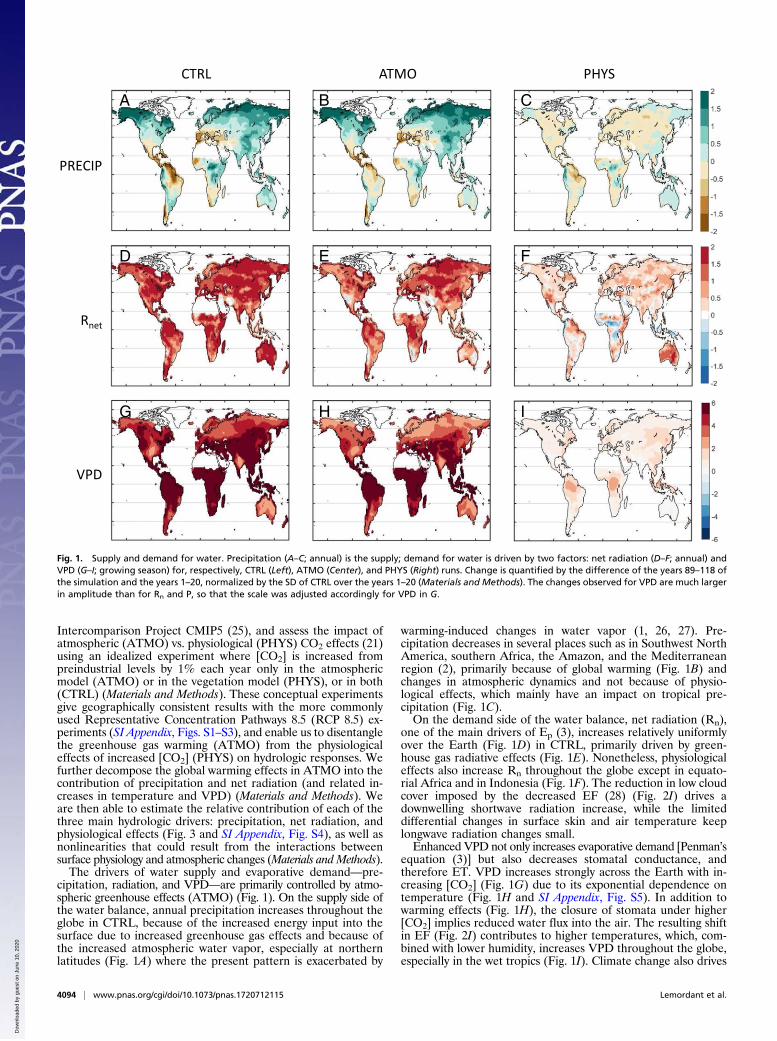
cipitation, radiation, and VPD––are primarily controlled by atmo-spheric greenhouse effects (ATMO) (Fig. 1). On the supply side ofthe water balance, annual precipitation increases throughout theglobe in CTRL, because of the increased energy input into thesurface due to increased greenhouse gas effects and because ofthe increased atmospheric water vapor, especially at northernlatitudes (Fig. 1A) where the present pattern is exacerbated by

warming-induced changes in water vapor (1, 26, 27). Pre-cipitation decreases in several places such as in Southwest NorthAmerica, southern Africa, the Amazon, and the Mediterraneanregion (2), primarily because of global warming (Fig. 1B) andchanges in atmospheric dynamics and not because of physio-logical effects, which mainly have an impact on tropical pre-cipitation (Fig. 1C).On the demand side of the water balance, net radiation (Rn),

one of the main drivers of Ep (3), increases relatively uniformlyover the Earth (Fig. 1D) in CTRL, primarily driven by green-house gas radiative effects (Fig. 1E). Nonetheless, physiologicaleffects also increase Rn throughout the globe except in equato-rial Africa and in Indonesia (Fig. 1F). The reduction in low cloudcover imposed by the decreased EF (28) (Fig. 2I) drives adownwelling shortwave radiation increase, while the limiteddifferential changes in surface skin and air temperature keeplongwave radiation changes small.Enhanced VPD not only increases evaporative demand [Penman’s

equation (3)] but also decreases stomatal conductance, andtherefore ET. VPD increases strongly across the Earth with in-creasing [CO2] (Fig. 1G) due to its exponential dependence ontemperature (Fig. 1H and SI Appendix, Fig. S5). In addition towarming effects (Fig. 1H), the closure of stomata under higher[CO2] implies reduced water flux into the air. The resulting shiftin EF (Fig. 2I) contributes to higher temperatures, which, com-bined with lower humidity, increases VPD throughout the globe,especially in the wet tropics (Fig. 1I). Climate change also drives

D

A

E

H

F

IG

B C

Fig. 1. Supply and demand for water. Precipitation (A–C; annual) is the supply; demand for water is driven by two factors: net radiation (D–F; annual) andVPD (G–I; growing season) for, respectively, CTRL (Left), ATMO (Center), and PHYS (Right) runs. Change is quantified by the difference of the years 89–118 ofthe simulation and the years 1–20, normalized by the SD of CTRL over the years 1–20 (Materials and Methods). The changes observed for VPD are much largerin amplitude than for Rn and P, so that the scale was adjusted accordingly for VPD in G.

4094 | www.pnas.org/cgi/doi/10.1073/pnas.1720712115 Lemordant et al.

Dow

nloa

ded

by g

uest

on

June

10,

202

0

differential land and ocean warming, reducing relative humidityover land (29), as highlighted in ATMO.

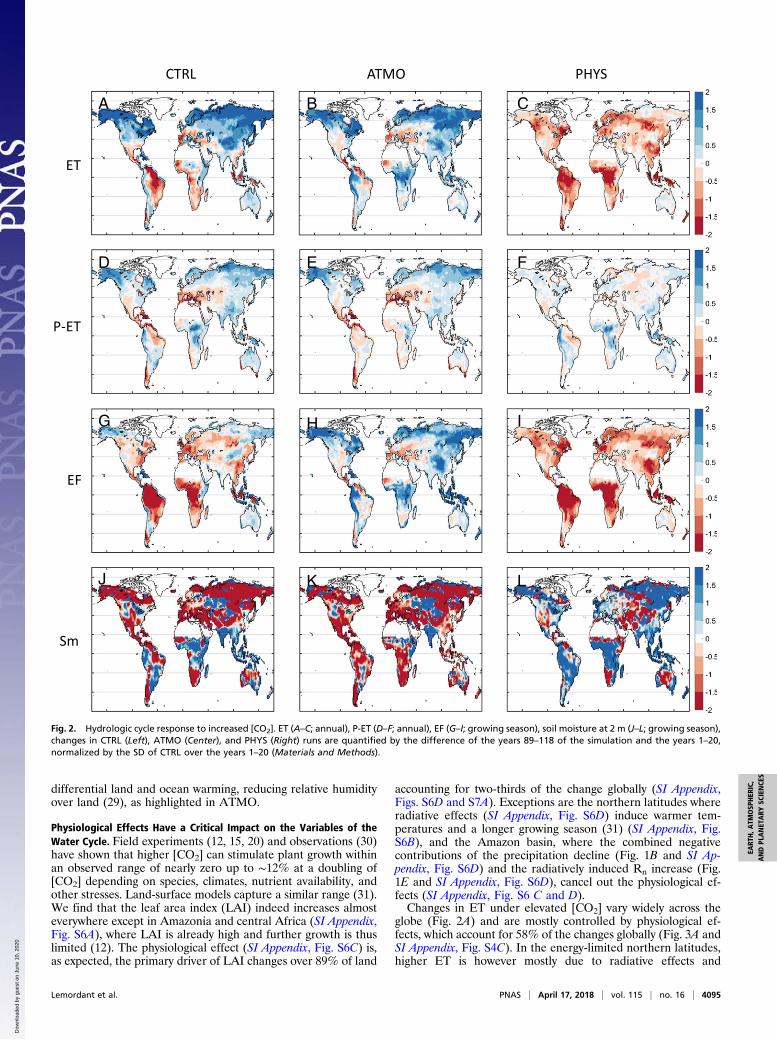
Physiological Effects Have a Critical Impact on the Variables of theWater Cycle. Field experiments (12, 15, 20) and observations (30)have shown that higher [CO2] can stimulate plant growth withinan observed range of nearly zero up to ∼12% at a doubling of[CO2] depending on species, climates, nutrient availability, andother stresses. Land-surface models capture a similar range (31).We find that the leaf area index (LAI) indeed increases almosteverywhere except in Amazonia and central Africa (SI Appendix,Fig. S6A), where LAI is already high and further growth is thuslimited (12). The physiological effect (SI Appendix, Fig. S6C) is,as expected, the primary driver of LAI changes over 89% of land

accounting for two-thirds of the change globally (SI Appendix,Figs. S6D and S7A). Exceptions are the northern latitudes whereradiative effects (SI Appendix, Fig. S6D) induce warmer tem-peratures and a longer growing season (31) (SI Appendix, Fig.S6B), and the Amazon basin, where the combined negativecontributions of the precipitation decline (Fig. 1B and SI Ap-pendix, Fig. S6D) and the radiatively induced Rn increase (Fig.1E and SI Appendix, Fig. S6D), cancel out the physiological ef-fects (SI Appendix, Fig. S6 C and D).Changes in ET under elevated [CO2] vary widely across the

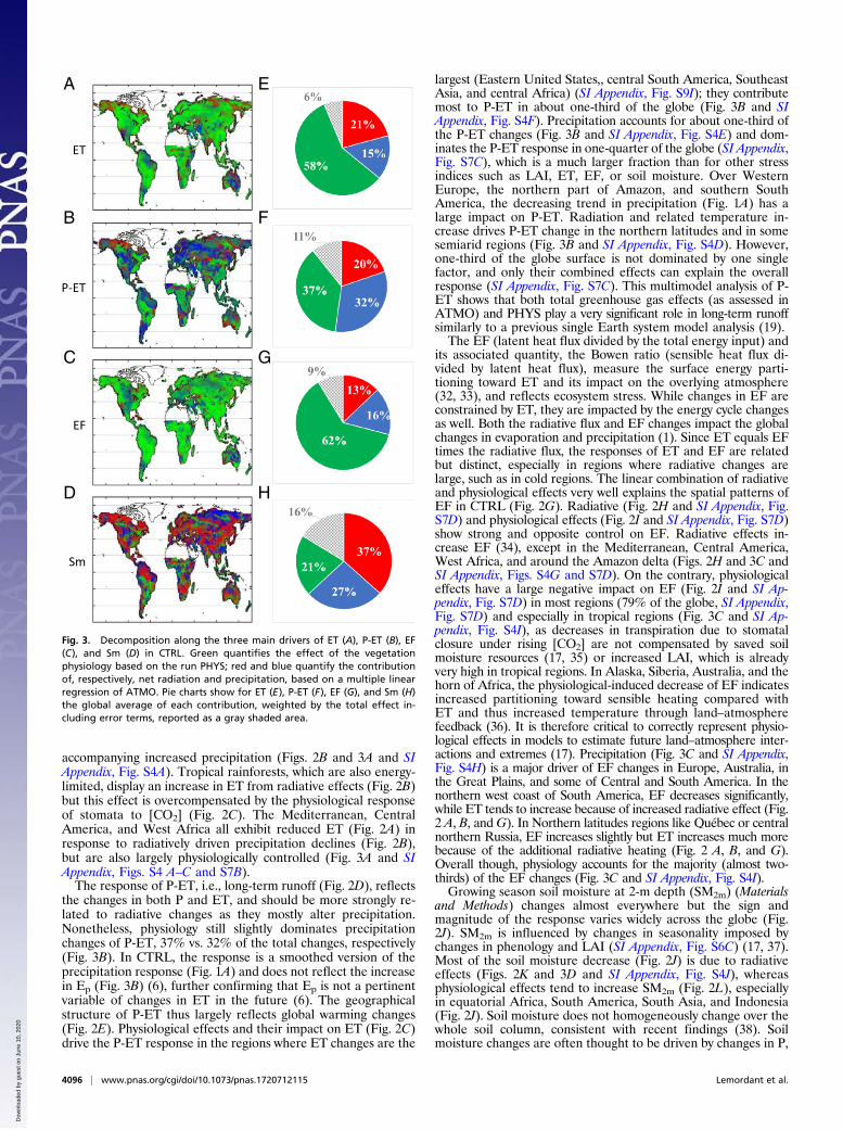
globe (Fig. 2A) and are mostly controlled by physiological ef-fects, which account for 58% of the changes globally (Fig. 3A andSI Appendix, Fig. S4C). In the energy-limited northern latitudes,higher ET is however mostly due to radiative effects and

A

D

G

J

B

E

H

K

C

F

I

L

Fig. 2. Hydrologic cycle response to increased [CO2]. ET (A–C; annual), P-ET (D–F; annual), EF (G–I; growing season), soil moisture at 2 m (J–L; growing season),changes in CTRL (Left), ATMO (Center), and PHYS (Right) runs are quantified by the difference of the years 89–118 of the simulation and the years 1–20,normalized by the SD of CTRL over the years 1–20 (Materials and Methods).

Lemordant et al. PNAS | April 17, 2018 | vol. 115 | no. 16 | 4095

EART

H,A

TMOSP

HER

IC,

ANDPL

ANET

ARY

SCIENCE

S

Dow

nloa

ded

by g

uest

on

June

10,

202

0

accompanying increased precipitation (Figs. 2B and 3A and SIAppendix, Fig. S4A). Tropical rainforests, which are also energy-limited, display an increase in ET from radiative effects (Fig. 2B)but this effect is overcompensated by the physiological responseof stomata to [CO2] (Fig. 2C). The Mediterranean, CentralAmerica, and West Africa all exhibit reduced ET (Fig. 2A) inresponse to radiatively driven precipitation declines (Fig. 2B),but are also largely physiologically controlled (Fig. 3A and SIAppendix, Figs. S4 A–C and S7B).The response of P-ET, i.e., long-term runoff (Fig. 2D), reflects

the changes in both P and ET, and should be more strongly re-lated to radiative changes as they mostly alter precipitation.Nonetheless, physiology still slightly dominates precipitationchanges of P-ET, 37% vs. 32% of the total changes, respectively(Fig. 3B). In CTRL, the response is a smoothed version of theprecipitation response (Fig. 1A) and does not reflect the increasein Ep (Fig. 3B) (6), further confirming that Ep is not a pertinentvariable of changes in ET in the future (6). The geographicalstructure of P-ET thus largely reflects global warming changes(Fig. 2E). Physiological effects and their impact on ET (Fig. 2C)drive the P-ET response in the regions where ET changes are the

largest (Eastern United States,, central South America, SoutheastAsia, and central Africa) (SI Appendix, Fig. S9I); they contributemost to P-ET in about one-third of the globe (Fig. 3B and SIAppendix, Fig. S4F). Precipitation accounts for about one-third ofthe P-ET changes (Fig. 3B and SI Appendix, Fig. S4E) and dom-inates the P-ET response in one-quarter of the globe (SI Appendix,Fig. S7C), which is a much larger fraction than for other stressindices such as LAI, ET, EF, or soil moisture. Over WesternEurope, the northern part of Amazon, and southern SouthAmerica, the decreasing trend in precipitation (Fig. 1A) has alarge impact on P-ET. Radiation and related temperature in-crease drives P-ET change in the northern latitudes and in somesemiarid regions (Fig. 3B and SI Appendix, Fig. S4D). However,one-third of the globe surface is not dominated by one singlefactor, and only their combined effects can explain the overallresponse (SI Appendix, Fig. S7C). This multimodel analysis of P-ET shows that both total greenhouse gas effects (as assessed inATMO) and PHYS play a very significant role in long-term runoffsimilarly to a previous single Earth system model analysis (19).The EF (latent heat flux divided by the total energy input) and

its associated quantity, the Bowen ratio (sensible heat flux di-vided by latent heat flux), measure the surface energy parti-tioning toward ET and its impact on the overlying atmosphere(32, 33), and reflects ecosystem stress. While changes in EF areconstrained by ET, they are impacted by the energy cycle changesas well. Both the radiative flux and EF changes impact the globalchanges in evaporation and precipitation (1). Since ET equals EFtimes the radiative flux, the responses of ET and EF are relatedbut distinct, especially in regions where radiative changes arelarge, such as in cold regions. The linear combination of radiativeand physiological effects very well explains the spatial patterns ofEF in CTRL (Fig. 2G). Radiative (Fig. 2H and SI Appendix, Fig.S7D) and physiological effects (Fig. 2I and SI Appendix, Fig. S7D)show strong and opposite control on EF. Radiative effects in-crease EF (34), except in the Mediterranean, Central America,West Africa, and around the Amazon delta (Figs. 2H and 3C andSI Appendix, Figs. S4G and S7D). On the contrary, physiologicaleffects have a large negative impact on EF (Fig. 2I and SI Ap-pendix, Fig. S7D) in most regions (79% of the globe, SI Appendix,Fig. S7D) and especially in tropical regions (Fig. 3C and SI Ap-pendix, Fig. S4I), as decreases in transpiration due to stomatalclosure under rising [CO2] are not compensated by saved soilmoisture resources (17, 35) or increased LAI, which is alreadyvery high in tropical regions. In Alaska, Siberia, Australia, and thehorn of Africa, the physiological-induced decrease of EF indicatesincreased partitioning toward sensible heating compared withET and thus increased temperature through land–atmospherefeedback (36). It is therefore critical to correctly represent physio-logical effects in models to estimate future land–atmosphere inter-actions and extremes (17). Precipitation (Fig. 3C and SI Appendix,Fig. S4H) is a major driver of EF changes in Europe, Australia, inthe Great Plains, and some of Central and South America. In thenorthern west coast of South America, EF decreases significantly,while ET tends to increase because of increased radiative effect (Fig.2 A, B, andG). In Northern latitudes regions like Québec or centralnorthern Russia, EF increases slightly but ET increases much morebecause of the additional radiative heating (Fig. 2 A, B, and G).Overall though, physiology accounts for the majority (almost two-thirds) of the EF changes (Fig. 3C and SI Appendix, Fig. S4I).Growing season soil moisture at 2-m depth (SM2m) (Materials

and Methods) changes almost everywhere but the sign andmagnitude of the response varies widely across the globe (Fig.2J). SM2m is influenced by changes in seasonality imposed bychanges in phenology and LAI (SI Appendix, Fig. S6C) (17, 37).Most of the soil moisture decrease (Fig. 2J) is due to radiativeeffects (Figs. 2K and 3D and SI Appendix, Fig. S4J), whereasphysiological effects tend to increase SM2m (Fig. 2L), especiallyin equatorial Africa, South America, South Asia, and Indonesia(Fig. 2J). Soil moisture does not homogeneously change over thewhole soil column, consistent with recent findings (38). Soilmoisture changes are often thought to be driven by changes in P,

A

B

C

D

E

F

G

H

Fig. 3. Decomposition along the three main drivers of ET (A), P-ET (B), EF(C), and Sm (D) in CTRL. Green quantifies the effect of the vegetationphysiology based on the run PHYS; red and blue quantify the contributionof, respectively, net radiation and precipitation, based on a multiple linearregression of ATMO. Pie charts show for ET (E), P-ET (F), EF (G), and Sm (H)the global average of each contribution, weighted by the total effect in-cluding error terms, reported as a gray shaded area.

4096 | www.pnas.org/cgi/doi/10.1073/pnas.1720712115 Lemordant et al.

Dow

nloa

ded

by g

uest

on

June

10,

202

0

but this is confirmed only over a very small fraction of the globe(Fig. 3D and SI Appendix, Figs. S4K and S7E), and, overall, soilmoisture changes have no unique global driver. Large fractionsof the globe are impacted by radiative changes, including theAmazon and most of western Europe (Fig. 3D and SI Appendix,Fig. S4J), where precipitation also declines (Fig. 1A). Vegetationand land–atmosphere interactions are the main drivers of soilmoisture changes in regions including South America, easternUnited States, Southeast Asia, and some places in central Africa(SI Appendix, Fig. S9O). In addition, soil moisture variations arestrongly nonlinear so that a linear decomposition does not ex-plain all of the features observed (SI Appendix, Figs. S1–S3 andS6E), emphasizing that predicting soil moisture is more com-plicated than other stress indices.

DiscussionThe control of precipitation on the future terrestrial water cycleis weak in general and represents the dominant control for only asmall fraction of the Earth, consistent with recent remote sensingobservations showing stronger vegetation response to atmosphericaridity compared with precipitation (39). In particular, precipita-tion trends are only a minor factor for biomass growth (as mea-sured by LAI, SI Appendix, Fig. S6 A–C) and energy partitioning(as indicated by EF, Fig. 2 G–I). We note that the response overthe Amazon basin is heavily influenced by net radiation changesrather than by physiological or precipitation effects (Fig. 3). Inenergy-limited ecosystems such as the Amazon, changes in radi-ation will become one of the primary drivers of transpiration andecosystem functioning (40). Our conclusions are not strongly af-fected by additional land-use and land-cover changes or the ad-dition of aerosols, as present in the RCP 8.5 simulations, whichoverall behave similarly to the simplified 1% yearly increase CO2experiments (SI Appendix, Fig. S1). Soil moisture appears to bethe most complex and nonlinear variable and is also affected byuncertain land-use and land-cover change and vegetation re-sponse (41). Our study illustrates how deeply the physiologicaleffects due to increasing atmospheric [CO2] impact the conti-nental water cycle. Contrary to previous wisdom, changes in pre-cipitation and radiation do not play the primary role in futuredrying and moistening in most regions. Rather, biosphere physi-ological effects and related biosphere–atmosphere interactions(42) are key for predicting future continental water stress asrepresented by ET, long-term runoff, EF, or leaf area index. Inturn, vegetation water stress largely regulates land carbon uptake(43), further emphasizing how tightly the future carbon and watercycles are coupled so that they cannot be evaluated in isolation.

Materials and MethodsWe used outputs from six Earth system models (ESM) from the idealizedsingle-forcing CMIP5 (25) experiments with [CO2] increasing either in theatmospheric model only, in the vegetation model only, or in both, at a rateof 1% per year. The combined vegetation and atmospheric model [CO2]increase is called CTRL (1pctCO2 in CMIP5 terminology). We call PHYS thevegetation model [CO2] increase with no atmospheric model increase(esmFixClim1 in the CMIP5 terminology). We call ATMO the converse simu-lations, with atmospheric and no vegetation [CO2] increase (esmFdbk1 inCMIP5 terminology). The three runs are replicas of the same experiment, inwhich the [CO2] is increased for 140 y by 1% each year starting from pre-industrial [CO2] levels in 1850 (except for HadGEM2-ES which starts in 1860).

The data are available for six models: bcc-csm1-1, CanESM2, CESM1-BGC,GFDL-ESM2M, HadGEM2-ES, and NorESM1-ME. For most of the models onlyone ensemble member is available for those experiments (r1i1p1 in theCMIP5 terminology), so we consider only one ensemble member per model.

The sum of ATMO and PHYS is very close to CTRL (SI Appendix, Figs. S2 andS3), indicating that the runs are indeed independent, and justifies this lineardecomposition. In particular, for example, rare and extreme events causedby increased warming do not significantly impact PHYS effects on the futuremean state in these simulations. Soil moisture, which shows more nonline-arities, is an exception. We also emphasize that because of slight differ-ences in each ensemble member initial condition, one should not expect toobtain a perfect match between the combined ATMO + PHYS and CTRL. In

particular, regional variations should be expected and due to the internalclimate variability.

These idealized runs differ from the more typical CMIP5 RepresentativeConcentration Pathways 8.5, an emission scenario from 2005 to 2100 thatincludes prescribed changes in land-use and land-cover scenarios, as well asaerosol and ozone forcing. Also, the [CO2] increase is different between RCP8.5 (ending at 936 ppm in 2100) and the 1% per year runs (ending at1,145 ppm after 140 y of simulation). For comparison with the idealized 1%runs, we combined RCP 8.5 with the data from historical runs simulating theperiod 1850–2005 (historical in CMIP5 terminology). The resulting data for1850–2100 are shown in SI Appendix, Figs. S1–S3, and are comparable interms of geographical features to the 1% simulations.

Our analysis is based onmonthly averaged outputs. We consider one valueof a givenwater stress indicator for each year, and suggest the use of themostrelevant period of the year for each variable and localization. It makes moresense to use annual average for precipitation and ET, and P-ET to obtain thetotal water fluxes––as ET is very small in cold winter regions. We also usethe annual average for the net radiation and LAI. However, summer is thedominant growing season whether in tropics, midlatitudes, or high lati-tudes, but not around the equator, and so plant soil moisture stress is morepresent and relevant in summer than at other times of year. Hence, we usethe summertime mean (i.e., June, July, and August for latitudes between[10; 90] and December, January, and February for latitudes between [−90;−15]) for EF, VPD, and soil moisture, three variables that indicate a stress,except around the equator (latitudes between [−15; 10]) where, in theCongo for instance, there are two dry/wet seasons. Around the equator,selecting only one season would thus lead to a subjective assessment ofdryness, as there is minimal dryness in the wet seasons, and ultimately theannual signal is dominated by the dry seasons. The [−15; 10] latitude rangewas chosen so that the transition with the local summer averaging zoneslooks smooth, and so that the equatorial range stays as small as possible.

We regrid each model to a common 1° × 1° grid to later compute theintermodel average. The change of a variable X is normalized beforethe intermodel averaging by the interannual variability and is calculated

according to the following formula: ΔX =Xfut −Xhist=σðXhistÞCTRL, where Xfut

is the mean of X over years 89–118 of the runs CTRL, PHYS and ATMO (re-spectively, 2070–2099 for RCP 8.5), Xhist is the mean of X over years 1–20(respectively, 1939–1968), and σðXhistÞCTRL is the SD of X over the same periodof the run CTRL. We have chosen the averaging periods so that the meanCO2 concentrations in all four sets of runs are similar (SI Appendix, Table S1).We then compute the standardized change ΔX intermodel average. Forcomparison, SI Appendix, Figs. S8 and S9 show for all of the variables pre-sented in Figs. 1 and 2 the change in ATMO and PHYS relative to CTRL:RUN=CTRL= ½Xfut   −  Xhist �RUN=½Xfut   −  Xhist �CTRL.

Net radiation is computed using the net downward minus upwardlongwave and shortwave radiation fluxes. EF is defined as the monthly ratioof the latent heat flux to the sum of the latent and the sensible heat fluxes.VPD is computed from the relative humidity and the saturation vaporpressure, calculated from the monthly averaged temperature. Soil moistureat 2m and at 30 cm are interpolated using themodel soil moisture profiles. Asthe number of layers varies across models, we first linearly interpolate theprofiles of each model and each annual data point (e.g., after the seasonalaveraging), extract the value at 2-m depth and 30-cm depth, and then applythe same routine as for the other variables.

SI Appendix, Fig. S11 shows the number of models that agree with thesign of the ΔX intermodel average. Only the soil moisture intermodel av-erage change shows wide areas of mismatch with individual modelchange sign.

We decompose changes in each water stress variable X (P-ET, LAI, etc.) intothree terms (Fig. 3 and SI Appendix, Fig. S4): the change due to the effect ofRn, the change due to the effect of P, and the change due to the effect ofthe physiology. Changes due to Rn are not differentiated from correlatedchanges in air temperature and VPD, as they are too collinear to yieldunique linear decomposition.

This translates into the following equation [1] decomposing changes inwater cycle variables, due to Rn and precipitation changes in ATMO andphysiological changes in PHYS (and related changes in atmospheric VPD andRn through land–atmosphere interactions, as seen in Figs. 1 and 2):

ΔX =��

∂X∂Rn

.ΔRn�ATMO

+�∂X∂P

.ΔP�ATMO

+ ½Decomposition  error�ATMO

�

+ ½ΔX�PHYS + ½Decomposition  error   into  ATMO &PHYS�. [1]

First we regrid X to 1 × 1° and temporally (annually except for the soilmoisture at 2 m) average it as for Fig. 2. Then we apply a multiple linear

Lemordant et al. PNAS | April 17, 2018 | vol. 115 | no. 16 | 4097

EART

H,A

TMOSP

HER

IC,

ANDPL

ANET

ARY

SCIENCE

S

Dow

nloa

ded

by g

uest

on

June

10,

202

0

regression of the variable X of ATMO with respect to the drivers P or Rn, overthe 140 y of the six models data of X. Hence we regress against 140 ×6 values for each grid point and each variable X, P, Rn. Those decomposedPHYS and ATMO runs help us uniquely define the sensitivity. This contrastswith CTRL where all variables are evolving jointly in response to both surfacephysiological and radiative changes so that a uniquely defined decomposi-tion is nearly impossible. The decomposition error terms are reported in SIAppendix, Figs. S2 and S3; the fraction of variance explained by the multiplelinear regression (R2) is in coherence with the fact that LAI and EF aredominated by physiological effects (Fig. 3C and SI Appendix, Fig. S6D), butlarge for P-ET (SI Appendix, Fig. S10).

A linear regression on net radiation and precipitation cannot account forall of the variance explained, as we did not include other modified variablessuch as temperature, relative humidity, or wind. However, given the verystrong correlation (nearly 1) of temperature with net radiation, a uniquelinear decomposition cannot be found. The other terms (relative humidity,wind, and nonlinearities), as well as nonlinearities and ensemble variations,explain the nonunity R2 (SI Appendix, Fig. S10). However, in most regions R2

is very high, emphasizing that precipitation and net radiation (and relatedtemperature changes) are the primary drivers of the change. In the CO2

physiological runs, precipitation changes as well as mean temperaturechanges are small (Fig. 1), so that it is fair to ignore precipitation influenceon the changes due to physiological effects.

It should also be noted that PHYS and ATMO are strictly independent andcannot have cross-correlation. The decomposition of CTRL into ATMO andPHYS is not perfect but works well, as shown in SI Appendix, Figs. S2 and S3.The effect of the linearization in ref. 1 in the independent PHYS andATMO runs is further compared with the full nonlinear response of the CTRLruns in SI Appendix, Figs. S2 and S3. ATMO and PHYS contribute quite in-dependently and linearly to CTRL (SI Appendix, Figs. S2 and S3). However, ifwe use the decomposition of ATMO changes along the precipitation and the

net radiation (as in Fig. 3 and SI Appendix, Fig. S4) to reconstruct anequivalent to CTRL, the result is satisfactory except for EF at northern lati-tudes and in eastern Africa (SI Appendix, Figs. S2 and S3), and especially forthe soil moisture (SI Appendix, Figs. S2 and S3), indicating nonlinearities,consistent with an overall low R2 (SI Appendix, Fig. S10). This further em-phasizes the difficulty to predict the change in soil moisture.

We end up with a triplet (R, G, B) with R, G, and B in [0; 1] for each pixeldefined as the absolute normalized sensitivity to net radiation, physiology,and precipitation changes, respectively:

R=

��� ∂X∂Rn.ΔRn

�ATMO

����� ∂X∂Rn.ΔRn

�ATMO

��+ ���∂X∂P .ΔP

�ATMO

��+ ��½ΔX�PHYS��, [2]

G=

��½ΔX�PHYS����� ∂X∂Rn.ΔRn

�ATMO

��+ ���∂X∂P .ΔP

�ATMO

��+ ��½ΔX�PHYS��, [3]

B=

���∂X∂P.ΔP

�ATMO

����� ∂X∂Rn.ΔRn

�ATMO

��+ ���∂X∂P.ΔP

�ATMO

��+ ��½ΔX�PHYS��.: [4]

The triplet (R, G, B) is used to color the pixel with the combination of (red,green, blue) in Fig. 3, as an indicator of absolute net radiation, physiology,and precipitation changes. On all plots we discard pixels where LAI is below0.2. Fig. 3 reports also pie charts of global averages of R, G, and B values,weighted by the total effect including error terms, reported in these piecharts as a dashed gray area.

ACKNOWLEDGMENTS. B.I.C. was supported by the NASA Modeling, Anal-ysis, and Prediction program, and Lamont-Doherty Earth ObservatoryContribution 8199.

1. Held IM, Soden BJ (2006) Robust responses of the hydrological cycle to globalwarming. J Clim 19:5686–5699.

2. Seager R, et al. (2014) Causes of increasing aridification of the mediterranean regionin response to rising greenhouse gases. J Clim 27:4655–4676.

3. Penman HL (1948) Natural evaporation from open water, bare soil and grass. Proc RSoc A 193:120–145.

4. Durack PJ, Wijffels SE, Matear RJ (2012) Ocean salinities reveal strong global watercycle intensification during 1950 to 2000. Science 336:455–458.

5. Greve P, Seneviratne SI (2015) Assessment of future changes in water availability andaridity. Geophys Res Lett 42:5493–5499.

6. Swann ALS, Hoffman FM, Koven CD, Randerson JT (2016) Plant responses to in-creasing CO2 reduce estimates of climate impacts on drought severity. Proc Natl AcadSci USA 113:10019–10024.

7. Milly PCD, Dunne KA (2016) Potential evapotranspiration and continental drying. NatClim Chang 6:946–949.

8. Byrne MP, O’Gorman PA (2015) The response of precipitation minus evapotranspi-ration to climate warming : Why the “‘wet-get-wetter, dry-get-drier’” scaling doesnot hold over land *. J Clim 28:8078–8092.

9. He J, Soden BJ (2016) A re-examination of the projected subtropical precipitationdecline. Nat Clim Chang 7:53–57.

10. Scheff J, Frierson DMW (2014) Scaling potential evapotranspiration with greenhousewarming. J Clim 27:1539–1558.

11. Good SP, Noone D, Bowen G (2015) Hydrologic connectivity constrains partitioning ofglobal terrestrial water fluxes. Science 349:175–177.

12. Norby RJ, Zak DR (2011) Ecological lessons from free-air CO2 enrichment (FACE) ex-periments. Annu Rev Ecol Evol Syst 42:181–203.

13. de Boer HJ, et al. (2011) Climate forcing due to optimization of maximal leaf con-ductance in subtropical vegetation under rising CO2. Proc Natl Acad Sci USA 108:4041–4046.

14. Lammertsma EI, et al. (2011) Global CO2 rise leads to reduced maximum stomatalconductance in Florida vegetation. Proc Natl Acad Sci USA 108:4035–4040.

15. Ainsworth EA, Long SP (2005) What have we learned from 15 years of free-airCO2 enrichment (FACE)? A meta-analytic review of the responses of photosynthe-sis, canopy properties and plant production to rising CO2. New Phytol 165:351–371.

16. Warren JM, et al. (2011) Ecohydrologic impact of reduced stomatal conductance inforests exposed to elevated CO2. Ecohydrology 4:196–210.

17. Lemordant L, Gentine P, Stéfanon M, Drobinski P, Fatichi S (2016) Modification ofland-atmosphere interactions by CO2 effects: Implications for summer dryness andheatwave amplitude. Geophys Res Lett 43:10240–10248.

18. Leuzinger S, Körner C (2007) Water savings in mature deciduous forest trees underelevated CO2. Glob Change Biol 13:2498–2508.

19. Betts RA, et al. (2007) Projected increase in continental runoff due to plant responsesto increasing carbon dioxide. Nature 448:1037–1041.

20. Mccarthy HR, et al. (2007) Temporal dynamics and spatial variability in the en-hancement of canopy leaf area under elevated atmospheric CO2. Glob Change Biol13:2479–2497.

21. Sellers PJ, et al. (1996) Comparison of radiative and physiological effects of doubledatmospheric CO_2 on climate. Science 271:1402–1406.

22. Berg A, et al. (2016) Land–atmosphere feedbacks amplify aridity increase over landunder global warming. Nat Clim Chang 6:869–874.

23. Scheff J, Frierson DMW (2015) Terrestrial aridity and its response to greenhousewarming across CMIP5 climate models. J Clim 28:5583–5600.

24. Greve P, et al. (2014) Global assessment of trends in wetting and drying over land. NatGeosci 7:716–721.

25. Taylor KE, Stouffer RJ (2011) Meehl G a (2007) a summary of the CMIP5 experimentdesign. WORLD 4:1–33.

26. Kapnick SB, Delworth TL (2013) Controls of global snow under a changed climate.J Clim 26:5537–5562.

27. Krasting JP, Broccoli AJ, Dixon KW, Lanzante JR (2013) Future changes in northernhemisphere snowfall. J Clim 26:7813–7828.

28. Gentine P, et al. (2013) A probabilistic bulk model of coupled mixed layer and con-vection. Part II: Shallow convection case. J Atmos Sci 70:1557–1576.

29. Byrne MP, O’Gorman PA (2016) Understanding decreases in land relative humiditywith global warming : Conceptual model and GCM simulations. J Clim 29:9045–9061.

30. Campbell JE, et al. (2017) Large historical growth in global terrestrial gross primaryproduction. Nature 544:84–87.

31. Zhu Z, et al. (2016) Greening of the earth and its drivers. Nat Clim Chang 6:791–795.32. Gentine P, Entekhabi D, Chehbouni A, Boulet G, Duchemin B (2007) Analysis of

evaporative fraction diurnal behaviour. Agric Meteorol 143:13–29.33. Gentine P, Entekhabi D, Polcher J (2011) The diurnal behavior of evaporative fraction

in the soil–vegetation–atmospheric boundary layer Continuum. J Hydrometeorol 12:1530–1546.

34. Hartmann DL (1994) Global Physical Climatology (Academic Press, San Diego), pp140–147.

35. Gray SB, et al. (2016) Intensifying drought eliminates the expected benefits of ele-vated carbon dioxide for soybean. Nat Plants 2:16132.

36. Seneviratne SI, et al. (2010) Investigating soil moisture-climate interactions in achanging climate: A review. Earth Sci Rev 99:125–161.

37. Boisier JP, Ciais P, Ducharne A, Guimberteau M (2015) Projected strengthening ofAmazonian dry season by constrained climate model simulations. Nat Clim Chang 5:656–660.

38. Berg A, Sheffield J, Milly PCD (2017) Divergent surface and total soil moisture pro-jections under global warming. Geophys Res Lett 44:236–244.

39. Konings AG, Williams AP, Gentine P (2017) Sensitivity of grassland productivity toaridity controlled by stomatal and xylem regulation. Nat Geosci 10:284–288.

40. Pieruschka R, Huber G, Berry JA (2010) Control of transpiration by radiation. Proc NatlAcad Sci USA 107:13372–13377.

41. Alkama R, Cescatti A (2016) Biophysical climate impacts of recent changes in globalforest cover. Science 351:600–604.

42. Green JK, et al. (2017) Regionally strong feedbacks between the atmosphere andterrestrial biosphere. Nat Geosci 10:410–414.

43. Poulter B, et al. (2014) Contribution of semi-arid ecosystems to interannual variabilityof the global carbon cycle. Nature 509:600–603.

4098 | www.pnas.org/cgi/doi/10.1073/pnas.1720712115 Lemordant et al.

Dow

nloa

ded

by g

uest

on

June

10,

202

0