credits: 10 learning hours: 100 sector: construction and
TRANSCRIPT

Page 1 of 63
TVET CERTIFICATE V in LAND SURVEYING
T T T S R 1 0 3 SURVEYING MEASUREMENT ADJUSTMENT
LSVSA501 PERFORM SURVEYING MEASUREMENT ADJUSTMENT
Credits: 10 Learning hours: 100
Sector: Construction and Building Services
Sub-sector: Land Surveying
Module Note Issue date: June, 2020
Purpose statement
This module describes the skills, knowledge and attitudes required to perform surveying measurement
adjustment. At the end of this module, participants will be able to identify principles of surveying
measurement, apply methods of surveying adjustment, and perform accuracy and precision of
measurements.
Page 2 of 63
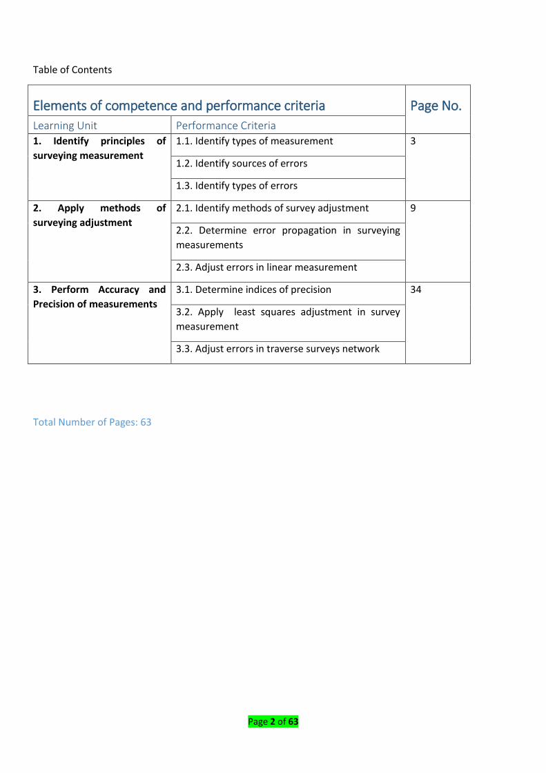
Table of Contents
Elements of competence and performance criteria Page No.
Learning Unit Performance Criteria
1. Identify principles of
surveying measurement
1.1. Identify types of measurement 3
1.2. Identify sources of errors
1.3. Identify types of errors
2. Apply methods of
surveying adjustment
2.1. Identify methods of survey adjustment 9
2.2. Determine error propagation in surveying
measurements
2.3. Adjust errors in linear measurement
3. Perform Accuracy and
Precision of measurements
3.1. Determine indices of precision 34
3.2. Apply least squares adjustment in survey
measurement
3.3. Adjust errors in traverse surveys network
Total Number of Pages: 63
Page 3 of 63
Learning Unit 1 – Identify Surveying Measurement principles
1. Introduction to surveying measurement and adjustment
We currently live in what is often termed the information age. Aided by new and emerging technologies,
data are being collected at unprecedented rates in all walks of life. For example, in the field of surveying,
total station instruments, global positioning system (GPS) equipment, digital metric cameras, and satellite
imaging systems are only some of the new instruments that are now available for rapid generation of vast
quantities of measured data.
Geographic Information Systems (GISs) have evolved concurrently with the development of these new
data acquisition instruments. GISs are now used extensively for management, planning, and design. They
are being applied worldwide at all levels of government, in business and industry, by public utilities, and in
private engineering and surveying offices. Implementation of a GIS depends upon large quantities of data
from a variety of sources, many of them consisting of observations made with the new instruments, such
as those noted above.
Before data can be utilized, however, whether for surveying and mapping projects, for engineering design,
or for use in a geographic information system, they must be processed. One of the most important aspects
of this is to account for the fact that no measurements are exact. That is, they always contain errors.
The steps involved in accounting for the existence of errors in measurements consist of (1) performing
statistical analyses of the observations to assess the magnitudes of their errors and to study their
distributions to determine whether or not they are within acceptable tolerances; and if the observations
are acceptable, (2) adjusting them so that they conform to exact geometric conditions or other required
constraints. Procedures for performing these two steps in processing measured data are principal subjects
of this book.
LO 1.1 – Identify Measurement Types
● Content/Topic 1 :Differentiate types of measurement
Measurements are defined as observations made to determine unknown quantities. They may be
classified as either direct or indirect.
Direct measurements are made by applying an instrument directly to the unknown quantity and
observing its value, usually by reading it directly from graduated scales on the device. Determining
the distance between two points by making a direct measurement using a graduated tape, or
measuring an angle by making a direct observation from the graduated circle of a theodolite or
total station instrument, are examples of direct measurements.
Indirect measurements are obtained when it is not possible or practical to make direct
measurements. In such cases the quantity desired is determined from its mathematical
relationship to direct measurements. Surveyors may, for example, measure angles and lengths of
lines between points directly and use these measurements to compute station coordinates. From
these coordinate values, other distances and angles that were not measured directly may be
derived indirectly by computation. During this procedure, the errors that were present in the
Page 4 of 63
original direct observations are propagated (distributed) by the computational process into the
indirect values. Thus, the indirect measurements (computed station coordinates, distances, and
angles) contain errors that are functions of the original errors. This distribution of errors is known
as error propagation. The analysis of how errors propagate is also a principal topic of this book.
L O 1.2. Identify Sources of Errors
Content/Topic 1 - Identification Of Errors In Measurements
By definition, an error is the difference between an observed value for a quantity and its true value, or
where E is the error in an observation, X the observed value, and its true value. It can be unconditionally
stated that (1) no observation is exact, (2) every observation contains errors, (3) the true value of an
observation is never known, and, therefore, (4) the exact error present is always unknown. These facts are
demonstrated by the following.
Errors in observations stem from three sources, and are classified accordingly.
Natural error: are caused by variations in wind, temperature, humidity, atmospheric pressure,
atmospheric refraction, gravity, and magnetic declination. An example is a steel tape whose length varies
with changes in temperature.
Instrumental errors: result from any imperfection in the construction or adjustment of instruments and
from the movement of individual parts. For example, the graduations
on a scale may not be perfectly spaced, or the scale may be warped. The effect of many instrumental
errors can be reduced, or even eliminated, by adopting proper surveying procedures or applying computed
corrections.
Personal errors: arise principally from limitations of the human senses of sight and touch. As an example, a
small error occurs in the observed value of a horizontal angle if the vertical crosshair in a total station
instrument is not aligned perfectly on the target, or if the target is the top of a rod that is being held
slightly out of plumb.
Page 5 of 63
L O 1.3 Identify Types of Errors
Content/Topic 1 – Identification Error Types
Errors in observations are of two types: systematic and random.
Systematic errors:
They arise from sources which act in a similar manner on observations.
The method of measurement, the instruments used and the physical conditions at the time of
measurements must all be considered in this respect.
So long as system conditions remain constant, the systematic errors will likewise remain constant. If
conditions change, the magnitudes of systematic errors also change. Because systematic errors
tend to accumulate, they are sometimes called cumulative errors.
Few examples of these errors include: Expansion of steel tapes, distance measuring (EDM)
instruments and collimation in a level.
Systematic errors are not revealed by taking the same measurement again with the same
instruments. The only way to check adequately for systematic error is to re-measure the quantity
by an entirely different method using different instruments.
Random errors:
Are those discrepancies remaining once blunders and systematic errors have been eliminated.
Even if a quantity is measured any times with the same instrument in the same way and if all
sources of systematic error have been removed, it is still highly unlikely that all results will be
identical. The differences caused mainly by limitations of instruments and observers are random
errors.
They are caused by factors beyond the control of the observer, obey the laws of probability, and
are sometimes called accidental errors. They are present in all surveying observations.
Page 6 of 63
The magnitudes and algebraic signs of random errors are matters of chance. There is no absolute
way to compute or eliminate them, but they can be estimated using adjustment procedures known
as least squares
Characteristics of random errors:
they are small errors and may occur more frequently than large ones
they can be positive or negative
Gross errors or mistakes:
These are observer blunders and are usually caused by misunderstanding the problem,
carelessness, fatigue, missed communication, or poor judgment...
These types of mistakes can occur at any stage of a survey when observing, booking,
computing or plotting and they would obviously have a very damaging effect on the results
if left uncorrected.
By following strictly a well-planned observing procedure it is possible to reduce the number
that occurs and then independent checks at each stage should show up those that have
been made.
Precision, accuracy, Reliability, Uncertainty
A discrepancy is the difference between two observed values of the same quantity. A small discrepancy
indicates there are probably no mistakes and random errors are small. However, small discrepancies do
not preclude the presence of systematic errors.
Precision:
Refers to the degree of refinement or consistency of a group of observations and is evaluated on
the basis of discrepancy size. If multiple observations are made of the same quantity and small
discrepancies result, this indicates high precision. The degree of precision attainable is dependent
on equipment sensitivity and observer skill.
The precision is expressed in terms of standard deviation of the error.
Accuracy:
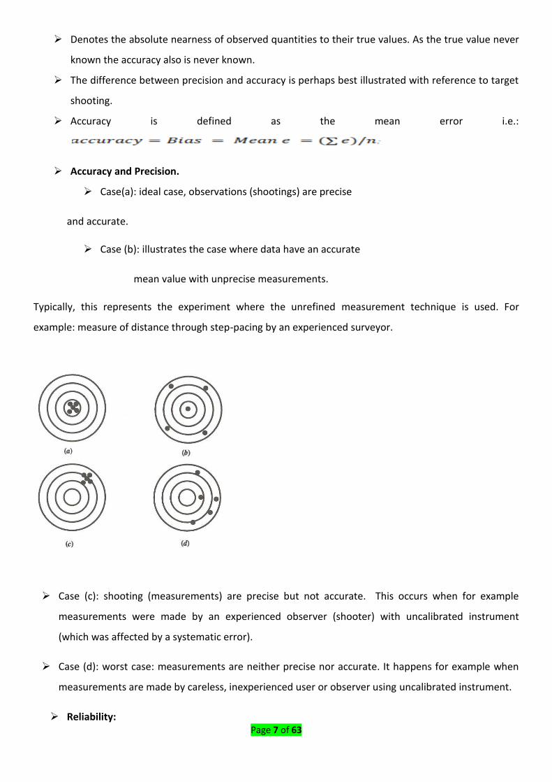
Page 7 of 63
Denotes the absolute nearness of observed quantities to their true values. As the true value never
known the accuracy also is never known.
The difference between precision and accuracy is perhaps best illustrated with reference to target
shooting.
Accuracy is defined as the mean error i.e.:
Accuracy and Precision.
Case(a): ideal case, observations (shootings) are precise
and accurate.
Case (b): illustrates the case where data have an accurate
mean value with unprecise measurements.
Typically, this represents the experiment where the unrefined measurement technique is used. For
example: measure of distance through step-pacing by an experienced surveyor.
Case (c): shooting (measurements) are precise but not accurate. This occurs when for example
measurements were made by an experienced observer (shooter) with uncalibrated instrument
(which was affected by a systematic error).
Case (d): worst case: measurements are neither precise nor accurate. It happens for example when
measurements are made by careless, inexperienced user or observer using uncalibrated instrument.
Reliability:

Page 8 of 63
Is a way of ensuring that any instrument used for measuring observations gives the same results
every time.
Uncertainty:
is a non-negative parameter characterizing the dispersion of the values attributed to a measured
quantity. It integrates both imprecision and inaccuracy. Uncertainty is expressed as root mean square error
(RMSE).
Assess Error Distribution During the Field Measurement
Then two basic rules are being used to distribute the error:
1—compass rule: error is distributed to the courses based on their length. Since course BM1-A is longer,
most of the correction belong to that course
2—transit rule: error is distributed to the courses based on latitude and longitude components of each
course; the course BM1-A runs from West to East, thus contains only longitude component and vice versa;
note that the courses do not change direction: transit is an equivalent to theodolite; assuming that
accuracy of angles is higher than accuracy of distances, then we prefer not to change the directions

Page 9 of 63
Learning Unit 2. Apply Methods of Surveying Adjustment
LO 2.1: Identify Methods of Surveying Adjustment
The methods of surveying adjustment are follow:
Chain and tape correction
Compass(Bowditch) rule
Transit rule
Adjustment by least squares
Content /Topic1 – Correction of chain and tape
In this method, steel tapes or wires are used to measure distance very accurately. Nowadays, EDM is being
used exclusively for accurate measurements but the steel tape still is of value for measuring limited lengths
for setting out purposes. Tape measurements require certain corrections to be applied to the measured
distance depending upon the conditions under which the measurements have been made. These
corrections are discussed below.
Systematic error correction in taping measurements
As like other observations there are three fundamental sources of errors in taping
1. Instrumental 2. Natural 3. Personal errors
1.1 Correction for Absolute Length
Due to manufacturing defects the absolute length of the tape may be different from its designated or
nominal length. Also with use the tape may stretch causing change in the length and it is imperative that
the tape is regularly checked under standard conditions to determine its absolute length. The correction
for absolute length or standardization is given by
Where
c = the correction per tape length,
l = the designated or nominal length of the tape, and
L= the measured length of the line.
Page 10 of 63
If the absolute length is more than the nominal length the sign of the correction is positive and vice versa.
1. Standard
a. Error occur when the length of the tape used is incorrect i.e. If the actual length of the tape
differs from its nominal graduated length due to defect in manufacture or repair.
b. Such errors are eliminated by checking the tape against a standard such as two marks
measured for the purpose so that the error per tape length is known.
1.2 Correction of systematic errors (length tape correction)
◦ If the error cannot be eliminated then a correction can be applied to remove the error.
◦ The correct lenth can be given by;
1.3 Slope correction
◦ It is already indicated that whenever slope distances are measured, they must be reduced to
horizontal plane.
◦ This can be done by computation from measured slope angle, or measured difference in
elevation, h of the two points in consideration.
standard
of Length
band usedLength of lengthmeasuredlengthCorrect
length recordedor measured
length tapenominal
length tapeactual
length measured toapplied be tocorrection
:
)'
'(
L
l'
l
C
Where
Ll
llC
l
l

Page 11 of 63
• H=L cos Or H=
The correction can be given by;
1.4 Tension Correction
Correct tension should be applied using a spring balance
If the standard tension is not applied a correection should be applied because the
lenght of the tape will have changed.
This correction is given by;
measuredlength
band for the elasticity of modulus sYoung'
band theof area sectional-cross
tensionstandard
tensionfield
;
)(
s
L
E
A
P
P
Where
LEA
PPCorrection
s
L
B
A
levelin difference
length measuredL
Where;
2
or ) cos1(
2
h
L
h-
LCorrection
Page 12 of 63
1.5 Temprature Correction
Correction is required if the tapes temprature, t at the time of measurement is not not equal to the
standard temprature, ts.
The temprature correction is given by;
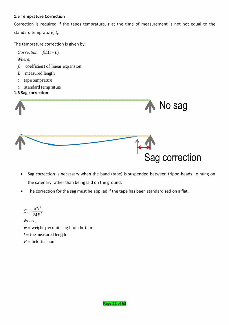
1.6 Sag correction
Sag correction is necessary when the band (tape) is suspended between tripod heads i.e hung on
the catenary rather than being laid on the ground.
The correction for the sag must be applied if the tape has been standardized on a flat.
Sag correction
No sag
e tempraturstandard
e tempraturtape
length measured
expansionlinear oft coefficien
;
)(
s
s
t
t
L
Where
ttLCorrection
tensionfield
length measured the
tape theoflength unit per weight
;
24 2
32
P
l
w
Where
P
lwCs

Page 13 of 63
Example 2.1. A line AB between the stations A and B was measured as 348.28 using a 20 m tape, too short
by 0.05 m. Determine the correct length of AB, the reduced horizontal length of AB if AB lay on a slope of 1
in 25, and the reading required to produce a horizontal distance of 22.86 m between two pegs, one being
0.56 m above the other.
Solution:
(a) Since the tape is too short by 0.05 m, actual length of AB will be less than the measured length. The
correction required to the measured length is

Page 14 of 63
Content /Topic2 – Correction by compass (Bowditch) Rule
The compass, or Bowditch rule adjusts the departures and latitudes of traverse courses in proportion to
their lengths. Although not as rigorous as the least-squares method; it does result in a logical distribution
of misclosures. Corrections by this method are made according to the following rules:
Note that the algebraic signs of the corrections are opposite those of the respective misclosures.
Example 10.4
Using the preliminary azimuths from Table 10.2 and lengths from Figure 10.1, compute departures and
latitudes, linear misclosure, and relative precision. Balance the departures and latitudes using the compass
rule.
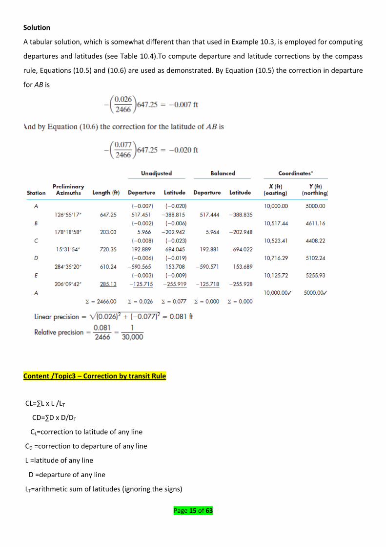
Page 15 of 63
Solution
A tabular solution, which is somewhat different than that used in Example 10.3, is employed for computing
departures and latitudes (see Table 10.4).To compute departure and latitude corrections by the compass
rule, Equations (10.5) and (10.6) are used as demonstrated. By Equation (10.5) the correction in departure
for AB is
Content /Topic3 – Correction by transit Rule
CL=∑L x L /LT
CD=∑D x D/DT
CL=correction to latitude of any line
CD =correction to departure of any line
L =latitude of any line
D =departure of any line
LT=arithmetic sum of latitudes (ignoring the signs)

Page 16 of 63
DT =arithmetic sum of departures (ignoring the signs)
∑L = total error (algebraic sum) in latitude,
∑D = total error (algebraic sum) in departure
Content /Topic4 – Correction by least square methods
It is a general practice in surveying to always have redundant observations as they help in detection of
mistakes or blunders. Redundant observations require a method which can yield a unique solution of the
model for which the observations have been made. The least squares method provides a general and
systematic procedure which yields a unique solution in all situations.
Assuming that all the observations are uncorrelated then the least squares method of adjustment is based
upon the following criterion: “The sum of the weighted squares of the residuals must be a minimum”. If υ
1, υ 2, υ 3, etc., are the residuals and ω 1, ω 2, ω 3, etc., are the weights then φ = ω 1 υ 1 2 + ω 2 υ 2 2 + ω
3 υ 3 2 +……+ ω n υ n 2 = a minimum
= Σω ν ii i n = ∑ = 1
a minimum.
The above condition which the residuals have to satisfy is in addition to the conditions which the adjusted
values have to satisfy for a given model
LO 2.2. Error Propagation in Surveying Measurements
Content/Topic 1 : Propagation Of Error In Surveying Measurement
Error propagation in surveying measurements
Error in a series
Error in a sum
Error in redundant measurement
Error in a Series Describes the error of multiple measurements with identical standard deviations, such as
measuring a 1000’ line with using a 100’ chain. E series En
E sum is the square root of the sum of each of the individual measurements squared It is used when there
are several measurements with differing standard errors 2222 E 2 E 3 ... E n E sum E 1
Error in Redundant Measurements If a measurement is repeated multiple times, the accuracy increases,
even if the measurements have the same value n E red. meas.

Page 17 of 63
If you learn one thing… With Errors of a Sum (or Series), each additional variable increases the total error of the network With Errors of Redundant Measurement, each redundant measurement decreases the error of the network. As the network becomes more complicated, accuracy can be maintained by increasing the number of redundant measurements
Introduction to Adjustments Adjustment - “A process designed to remove inconsistencies in measured or computed quantities by applying derived corrections to compensate for random, or accidental errors, such errors not being subject to systematic corrections
LO 2.3- Identify Methods of Surveying Adjustment by application
Content/Topic 1 : Correction for tape measurement
Tape measurements require certain corrections to be applied to the measured distance
depending upon the conditions under which the measurements have been made. These
corrections are discussed below
Correction for Absolute Length Due to manufacturing defects the absolute length of the
tape may be different from its designated or nominal length. Also with use the tape may
stretch causing change in the length and it is imperative that the tape is regularly checked
under standard conditions to determine its absolute length. The correction for absolute
length or standardization is given by
Where
c = the correction per tape length,
l = the designated or nominal length of the tape, and
L= the measured length of the line.
If the absolute length is more than the nominal length the sign of the correction is positive
and vice versa
Page 18 of 63
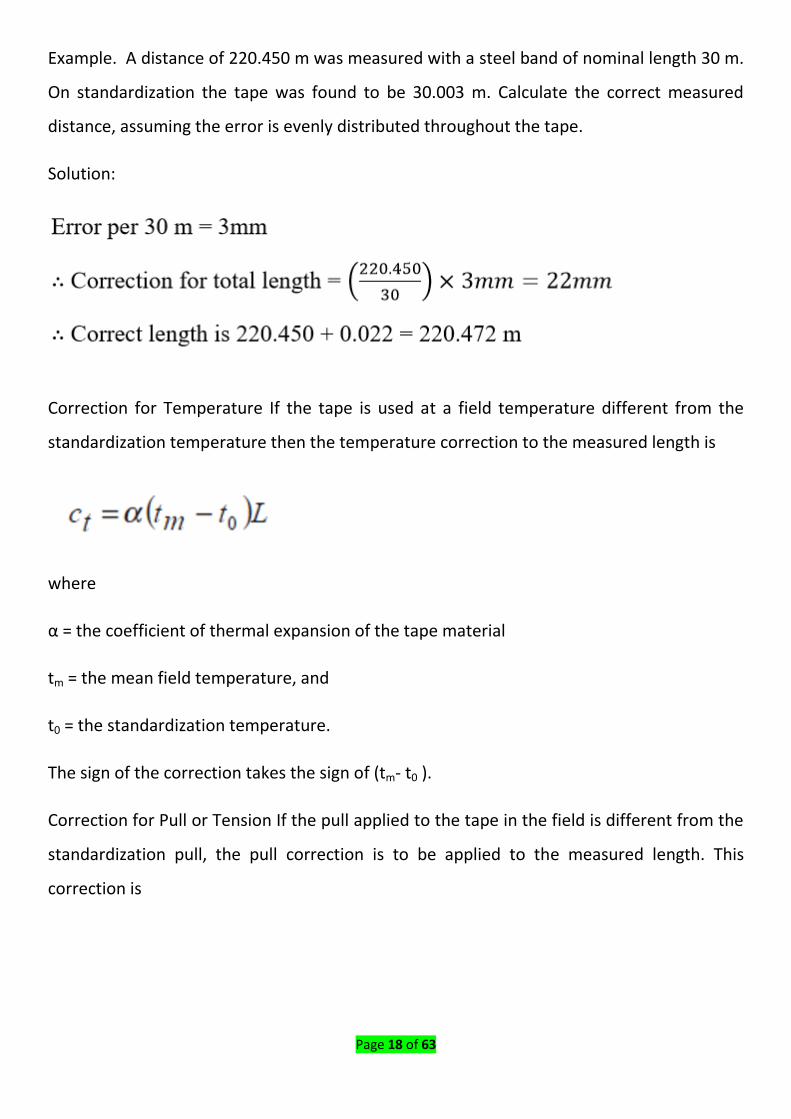
Example. A distance of 220.450 m was measured with a steel band of nominal length 30 m.
On standardization the tape was found to be 30.003 m. Calculate the correct measured
distance, assuming the error is evenly distributed throughout the tape.
Solution:
Correction for Temperature If the tape is used at a field temperature different from the
standardization temperature then the temperature correction to the measured length is
where
α = the coefficient of thermal expansion of the tape material
tm = the mean field temperature, and
t0 = the standardization temperature.
The sign of the correction takes the sign of (tm- t0 ).
Correction for Pull or Tension If the pull applied to the tape in the field is different from the
standardization pull, the pull correction is to be applied to the measured length. This
correction is
Page 19 of 63
where
P = the pull applied during the measurement,
P0 = the standardization pull,
A = the area of cross-section of the tape, and
E = the Young‘s modulus for the tape material.
The sign of the correction is same as that of (P – P0).
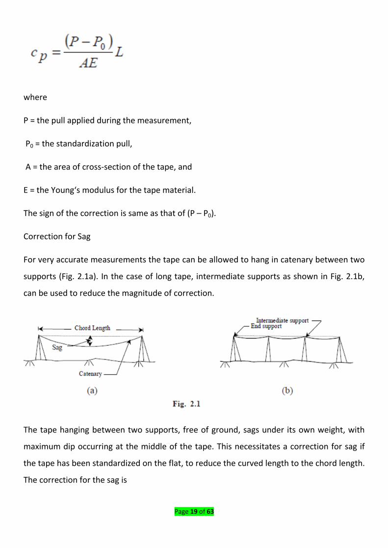
Correction for Sag
For very accurate measurements the tape can be allowed to hang in catenary between two
supports (Fig. 2.1a). In the case of long tape, intermediate supports as shown in Fig. 2.1b,
can be used to reduce the magnitude of correction.
The tape hanging between two supports, free of ground, sags under its own weight, with
maximum dip occurring at the middle of the tape. This necessitates a correction for sag if
the tape has been standardized on the flat, to reduce the curved length to the chord length.
The correction for the sag is
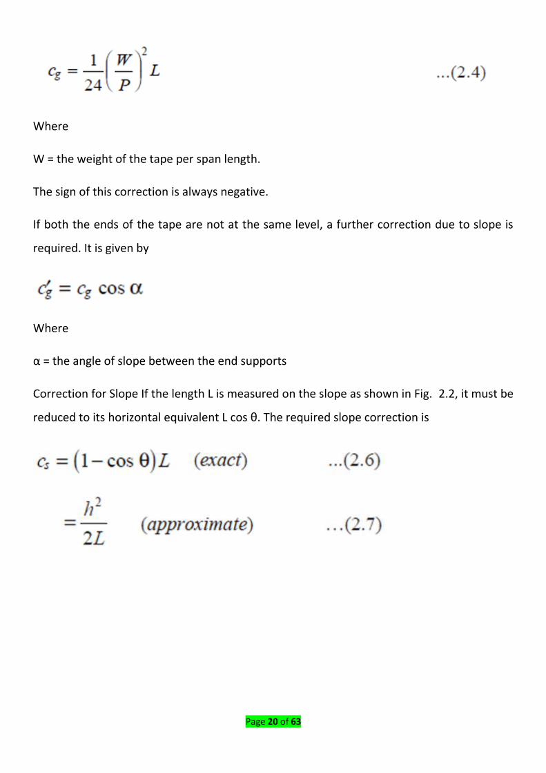
Page 20 of 63
Where
W = the weight of the tape per span length.
The sign of this correction is always negative.
If both the ends of the tape are not at the same level, a further correction due to slope is
required. It is given by
Where
α = the angle of slope between the end supports
Correction for Slope If the length L is measured on the slope as shown in Fig. 2.2, it must be
reduced to its horizontal equivalent L cos θ. The required slope correction is

Page 21 of 63
Where
θ = the angle of the slope, and
h = the difference in elevation of the ends of the tape.
The sign of this correction is always negative
Correction for Alignment If the intermediate points are not in correct alignment with ends
of the line, a correction for alignment given below, is applied to the measured length (Fig.
2.3).
Where
d = the distance by which the other end of the tape is out of alignment.
The correction for alignment is always negative
Page 22 of 63
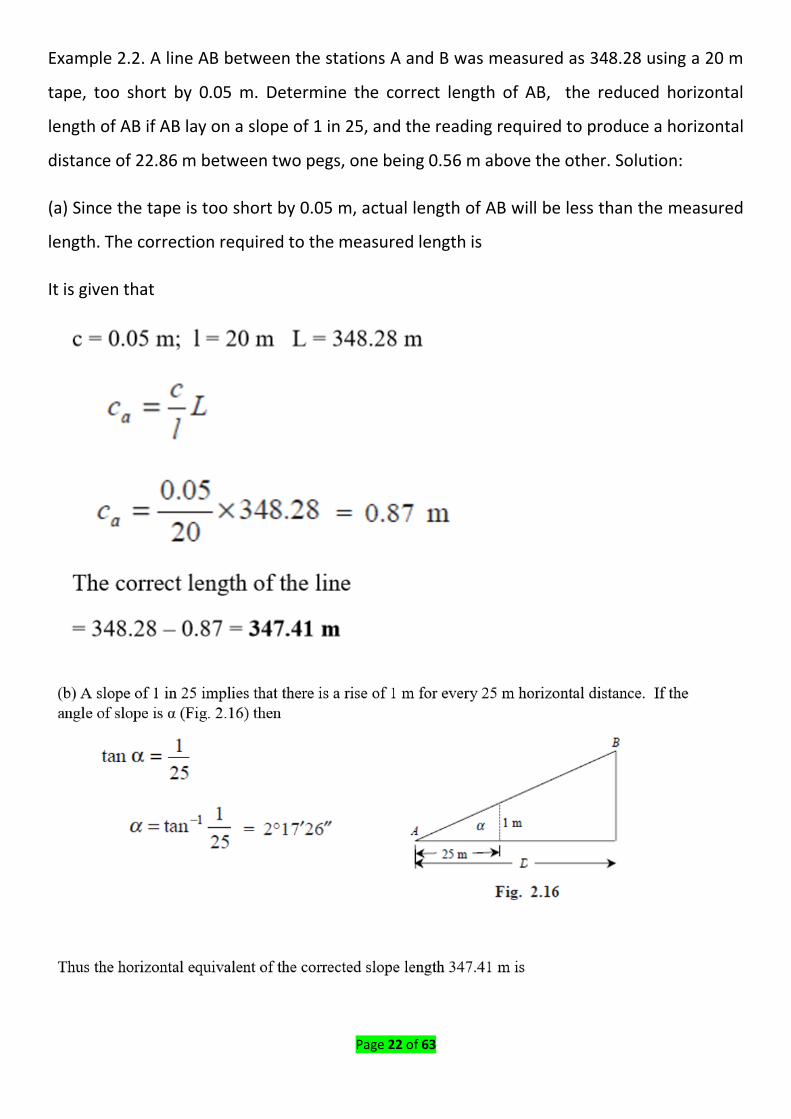
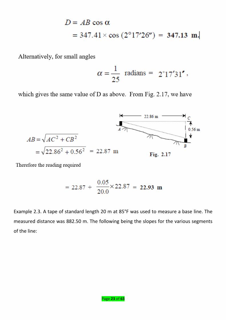
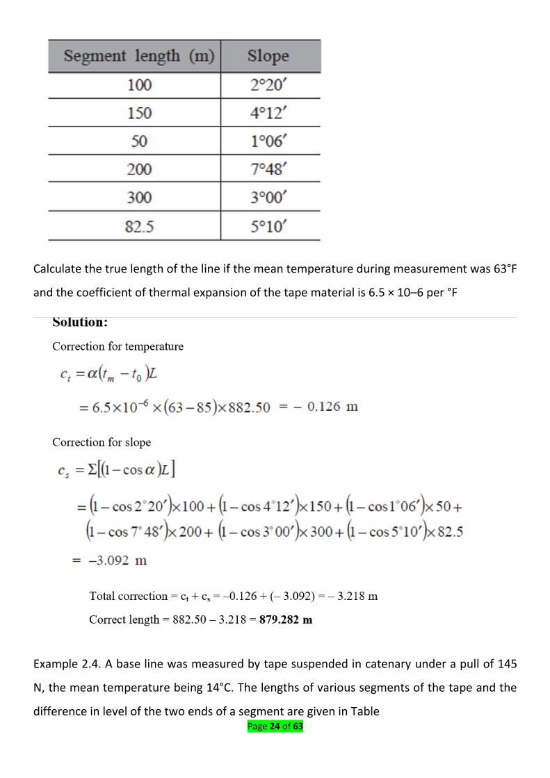
Example 2.2. A line AB between the stations A and B was measured as 348.28 using a 20 m
tape, too short by 0.05 m. Determine the correct length of AB, the reduced horizontal
length of AB if AB lay on a slope of 1 in 25, and the reading required to produce a horizontal
distance of 22.86 m between two pegs, one being 0.56 m above the other. Solution:
(a) Since the tape is too short by 0.05 m, actual length of AB will be less than the measured
length. The correction required to the measured length is
It is given that
Page 23 of 63
Example 2.3. A tape of standard length 20 m at 85°F was used to measure a base line. The
measured distance was 882.50 m. The following being the slopes for the various segments
of the line:
Page 24 of 63
Calculate the true length of the line if the mean temperature during measurement was 63°F
and the coefficient of thermal expansion of the tape material is 6.5 × 10⁻⁶ per °F
Example 2.4. A base line was measured by tape suspended in catenary under a pull of 145
N, the mean temperature being 14°C. The lengths of various segments of the tape and the
difference in level of the two ends of a segment are given in Table

Page 25 of 63
If the tape was standardized on the flat under a pull of 95 N at 18°C determine the correct
length of the line. Take
Cross-sectional area of the tape = 3.35 mm2
Mass of the tape = 0.025 kg/m
Coefficient of linear expansion = 0.9 × 10⁻⁶ per °C
Young‘s modulus = 14.8 × 10⁴ MN/m2
Solution:
It is given that
Page 26 of 63

Page 27 of 63
Correct length = 119.631 – 0.0056 = 119.6254 m
Page 28 of 63
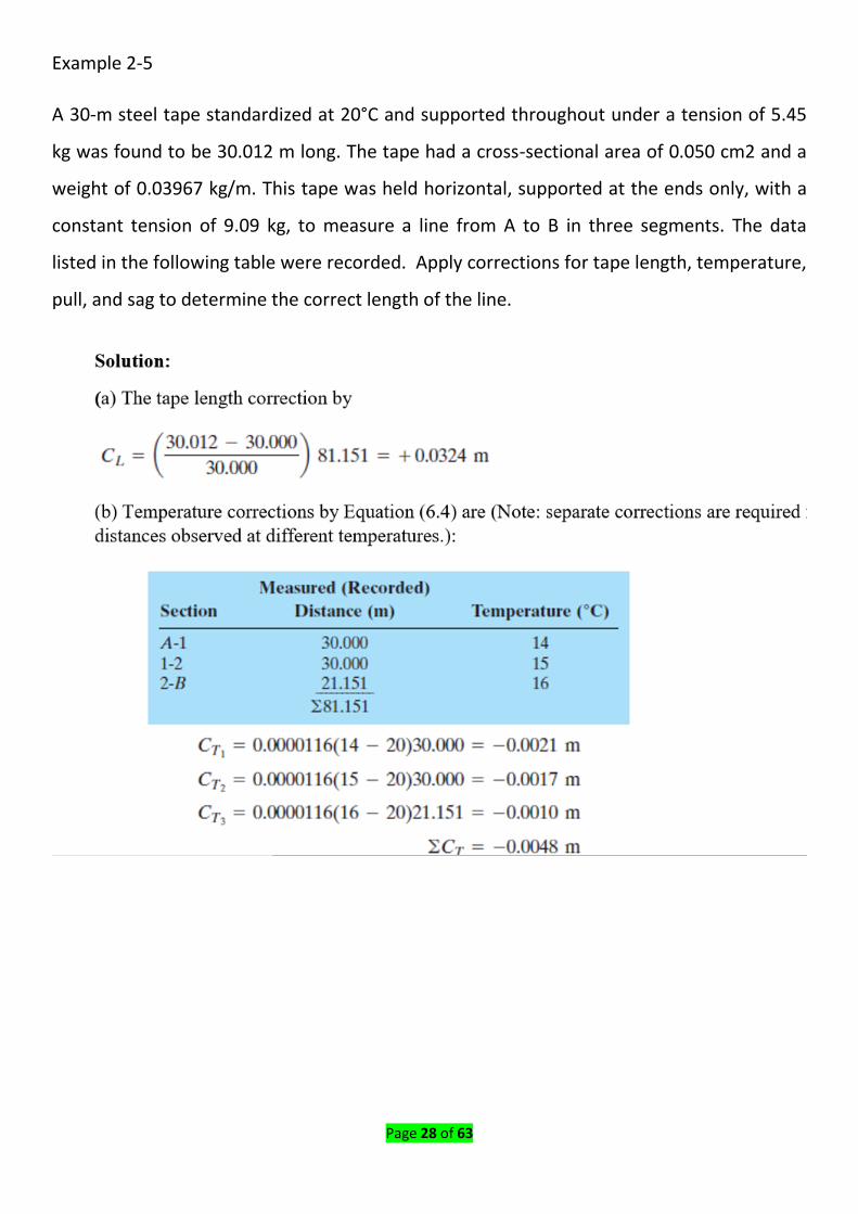
Example 2-5
A 30-m steel tape standardized at 20°C and supported throughout under a tension of 5.45
kg was found to be 30.012 m long. The tape had a cross-sectional area of 0.050 cm2 and a
weight of 0.03967 kg/m. This tape was held horizontal, supported at the ends only, with a
constant tension of 9.09 kg, to measure a line from A to B in three segments. The data
listed in the following table were recorded. Apply corrections for tape length, temperature,
pull, and sag to determine the correct length of the line.

Page 29 of 63
(e) Finally, corrected distance AB is obtained by adding all corrections to the measured
distance, or
AB = 81.151 + 0.0324 - 0.0048 + 0.0030 - 0.0504 = 81.131 m
Home work
1) A 100-ft steel tape standardized at 68°F and supported throughout under a tension of 20
lb was found to be 100.012 ft long. The tape had a cross-sectional area of0.0078 in.2 and a
weight of 0.0266 lb/ft. This tape is used to lay off a horizontal distance CD of exactly 175.00
ft. The ground is on a smooth 3% grade, thus the tape will be used fully supported.
Determine the correct slope distance to layoff if a pull of 15 lb is used and the temperature
is 87°F.
2) A tape of 30 m length suspended in catenary measured the length of a base line. After
applying all corrections the deduced length of the base line was 1462.36 m. Later on it was
found that the actual pull applied was 155 N and not the 165 N as recorded in the field
book. Correct the deduced length for the incorrect pull. The tape was standardized on the
flat under a pull of 85 N having a mass of 0.024 kg/m and cross-sectional area of 4.12 mm2.
Page 30 of 63
The Young‘s modulus of the tape material is 152000 MN/ m2 and the acceleration due to
gravity is 9.806 m/s2.
Content/Topic 2 - Identification Of Systematic And Random Error In Differencial Levelling
2.3.1 Systematic errors in differential levelling
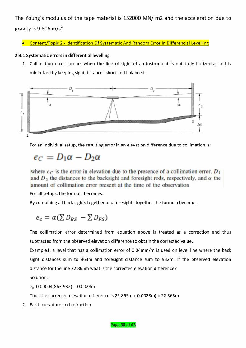
1. Collimation error: occurs when the line of sight of an instrument is not truly horizontal and is
minimized by keeping sight distances short and balanced.
For an individual setup, the resulting error in an elevation difference due to collimation is:
For all setups, the formula becomes:
By combining all back sights together and foresights together the formula becomes:
The collimation error determined from equation above is treated as a correction and thus
subtracted from the observed elevation difference to obtain the corrected value.
Example1: a level that has a collimation error of 0.04mm/m is used on level line where the back
sight distances sum to 863m and foresight distance sum to 932m. If the observed elevation
distance for the line 22.865m what is the corrected elevation difference?
Solution:
ec=0.00004(863-932)= -0.0028m
Thus the corrected elevation difference is 22.865m-(-0.0028m) = 22.868m
2. Earth curvature and refraction

Page 31 of 63
As the line of sight extends from an instrument, the level surface curves down and away. This
condition always causes rod readings to bee to high. Curvature effect.
As the line of sight extends from instrument. Refraction bends it toward the Earth’s surface,
causing readings to be too low. Refraction effect.
The combined effect of earth curvature and refraction on an individual sight always causes a
rod reading to too high by an amount approximated as: Where hCR is the
error in reading (in feet or meters), CR is 0.0675 when D is in units of meters or 0.0206 when D
is in units of feet, and D is the individual sight distance.
The effect of this error on a single elevation difference is minimized by keeping backsight and
foresight distances short and equal.
For the unequal sight distances, the resulting error is expressed as:
Where eCR is the error due to curvature and refraction and D1 and D2 are the individual back
sight and foresight distances that occur in a line of levels.
The equation above is the correction and is subtracted from the observed elevation difference to get the
corrected value. The sum of the backsight and foresight
distances of the whole level line will yield incorrect results, these distances should be squared before
they are summed.
Example2: An elevation difference between two stations on a hillside is determined to be 1.256m.
What would be the error in the elevation difference and the corrected elevation difference if the back
sight distance were 100m and the foresight distance 20m only?
Solution: substituting the distance into equation above and using CR=0.0675 gives us
From this the corrected elevation difference is h= 1.256m-0.0006m=1.255m
For the line of differential leveling, the combined effect of this error is:

Page 32 of 63
Regrouping back sight and fore sight distances:
3. Combined effects of systematic errors on elevation differences for one instrument set up, a
corrected elevation difference h:
Where r1 is the back sight rod reading, r2 is the foresight reading, others terms are defined as equation
(3):
For a line of levels, the corrected elevation differences h become:
rBs
and rFs are respectively the sum of all back sight and fore sight, D2 FS are respectively the sum of
squares of back sights and foresights of whole leveling.
Content/Topic 2 – Random errors in differencial leveling
Reading rod errors
Rod reading errors for any individual sight distance D is: r= Dr/D
Where r/D is the estimated error in the rod reading per unit length of sight distance and D is the length of
sight distance.
Instrument-leveling errors
The estimated error in leveling for an automatic compensator or level vial is generally given in the technical
data for each instrument.
For precise levels, this information is listed in arc second or an estimated elevation error for a given
distance: for example: the estimated error of 1.5mm/km correspond to: 1.5/1,000,000*p=0.3”. This
error ranges between 0.1”and 0.2” for a precise level and 10” for a less precise level. N.B:
Page 33 of 63
P=206264.8”/radian which comes from the fact that 206264.8”=1radian
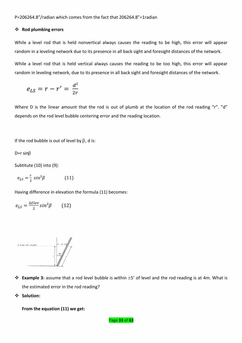
Rod plumbing errors
While a level rod that is held nonvertical always causes the reading to be high, this error will appear
random in a leveling network due to its presence in all back sight and foresight distances of the network.
While a level rod that is held vertical always causes the reading to be too high, this error will appear
random in leveling network, due to its presence in all back sight and foresight distances of the network.
Where D is the linear amount that the rod is out of plumb at the location of the rod reading “r”. ”d”
depends on the rod level bubble centering error and the reading location.
If the rod bubble is out of level by , d is:
D=r sin
Subtitute (10) into (9):
Having difference in elevation the formula (11) becomes:
Example 3: assume that a rod level bubble is within 5’ of level and the rod reading is at 4m. What is
the estimated error in the rod reading?
Solution:
From the equation (11) we get:
Page 34 of 63
Learning Unit.3. Perform Accuracy and Precision of Measurements
LO 3.1. Adequate Determination Of Indices Of Precision
Content /Topic3 - Determination of Indices Of Precision
Measures of central tendency are computed statistical quantities that give an indication of the value within
a data set that tends to exist at the center. The arithmetic mean, the median, and the mode are three such
measures. They are described as follows:
ARITHMETIC MEAN. For a set of n observations, y1, y2,...,yn, this is the average of the observations. Its
value, is computed from the equation:
(2.1)
Median.
As mentioned previously, this is the midpoint of a sample set when arranged in ascending or descending
order. One-half of the data are above the median and one-half are below it. When there are an odd
number of quantities, only one such value satisfies this condition. For a data set with an even number of
quantities, the average of the two observations that straddle the midpoint is used to represent the
median.
Mode.
Within a sample of data, the mode is the most frequently occurring value. It is seldom used in surveying
because of the relatively small number of values observed in a typical set of observations. In small sample
sets, several different values may occur with the same frequency, and hence the mode can be meaningless
as a measure of central tendency.
True Value, µ:
A quantity’s theoretically correct or exact value
Error, ε:
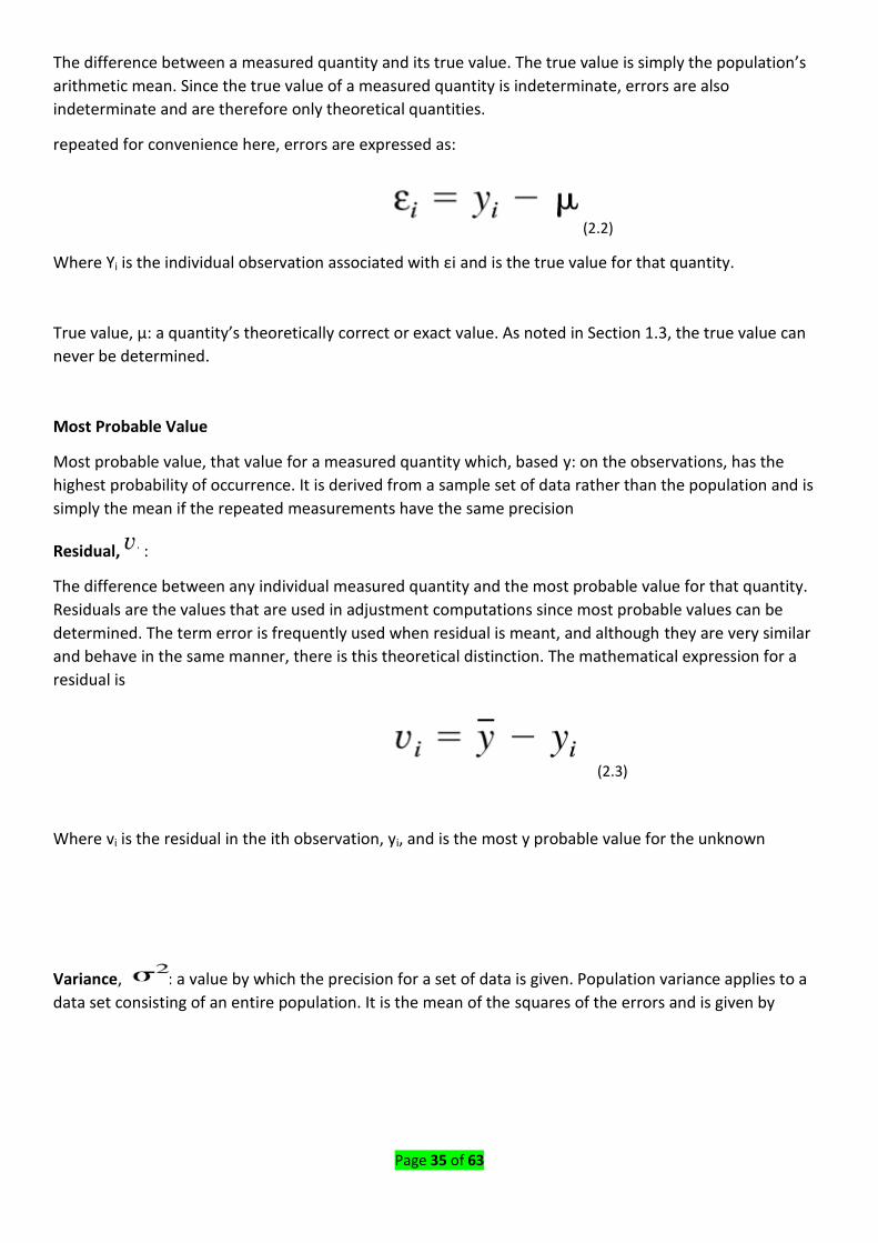
Page 35 of 63
The difference between a measured quantity and its true value. The true value is simply the population’s
arithmetic mean. Since the true value of a measured quantity is indeterminate, errors are also
indeterminate and are therefore only theoretical quantities.
repeated for convenience here, errors are expressed as:
(2.2)
Where Yi is the individual observation associated with εi and is the true value for that quantity.
True value, µ: a quantity’s theoretically correct or exact value. As noted in Section 1.3, the true value can
never be determined.
Most Probable Value
Most probable value, that value for a measured quantity which, based y: on the observations, has the
highest probability of occurrence. It is derived from a sample set of data rather than the population and is
simply the mean if the repeated measurements have the same precision
Residual, :
The difference between any individual measured quantity and the most probable value for that quantity.
Residuals are the values that are used in adjustment computations since most probable values can be
determined. The term error is frequently used when residual is meant, and although they are very similar
and behave in the same manner, there is this theoretical distinction. The mathematical expression for a
residual is
(2.3)
Where vi is the residual in the ith observation, yi, and is the most y probable value for the unknown
Variance, : a value by which the precision for a set of data is given. Population variance applies to a
data set consisting of an entire population. It is the mean of the squares of the errors and is given by

Page 36 of 63
(2.4)
Sample variance applies to a sample set of data. It is an unbiased estimate for the population variance
given in Equation above and is calculated as
(2.5)
Standard error, :
the square root of the population variance. From Equation (2.4) and this definition, the following equation
is written for the standard error:
(2.6)
Standard Deviation, S: the square root of the sample variance. It is calculated using the expression
(2.7)
where S is the standard deviation, n -1 the degrees of freedom or number of redundancies, and
the sum of the squares of residuals. Standard deviation is an estimate for the
standard error of the population. Since the standard error cannot be determined, the standard deviation is
a practical expression for the precision of a sample set of data. Residuals are used rather than errors
because they can be calculated from most probable values, whereas errors cannot be determined. Again,
as discussed in Section 3.5, for a sample data set, 68.3% of the observations will theoretically lie between
the most probable value plus and minus the standard deviation, S. The meaning of this statement will be
clarified in an example that follows.
Standard Deviation Of The Mean: the error in the mean computed from a sample set of measured values
that results because all measured values contain errors. The standard deviation of the mean is computed
from the sample standard deviation according to the equation
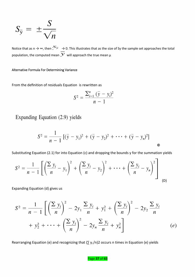
Page 37 of 63
Notice that as n → ∞, then → 0. This illustrates that as the size of Sy the sample set approaches the total
population, the computed mean will approach the true mean µ
Alternative Formula For Determining Variance
From the definition of residuals Equation is rewritten as
©
Substituting Equation (2.1) for into Equation (c) and dropping the bounds y for the summation yields
(D)
Expanding Equation (d) gives us
Rearranging Equation (e) and recognizing that (∑ yi /n)2 occurs n times in Equation (e) yields
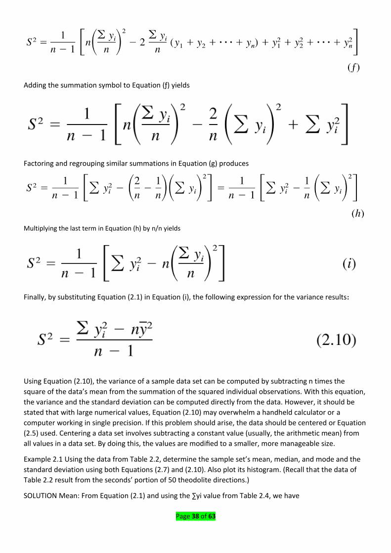
Page 38 of 63
Adding the summation symbol to Equation (ƒ) yields
Factoring and regrouping similar summations in Equation (g) produces
Multiplying the last term in Equation (h) by n/n yields
Finally, by substituting Equation (2.1) in Equation (i), the following expression for the variance results:
Using Equation (2.10), the variance of a sample data set can be computed by subtracting n times the
square of the data’s mean from the summation of the squared individual observations. With this equation,
the variance and the standard deviation can be computed directly from the data. However, it should be
stated that with large numerical values, Equation (2.10) may overwhelm a handheld calculator or a
computer working in single precision. If this problem should arise, the data should be centered or Equation
(2.5) used. Centering a data set involves subtracting a constant value (usually, the arithmetic mean) from
all values in a data set. By doing this, the values are modified to a smaller, more manageable size.
Example 2.1 Using the data from Table 2.2, determine the sample set’s mean, median, and mode and the
standard deviation using both Equations (2.7) and (2.10). Also plot its histogram. (Recall that the data of
Table 2.2 result from the seconds’ portion of 50 theodolite directions.)
SOLUTION Mean: From Equation (2.1) and using the ∑yi value from Table 2.4, we have
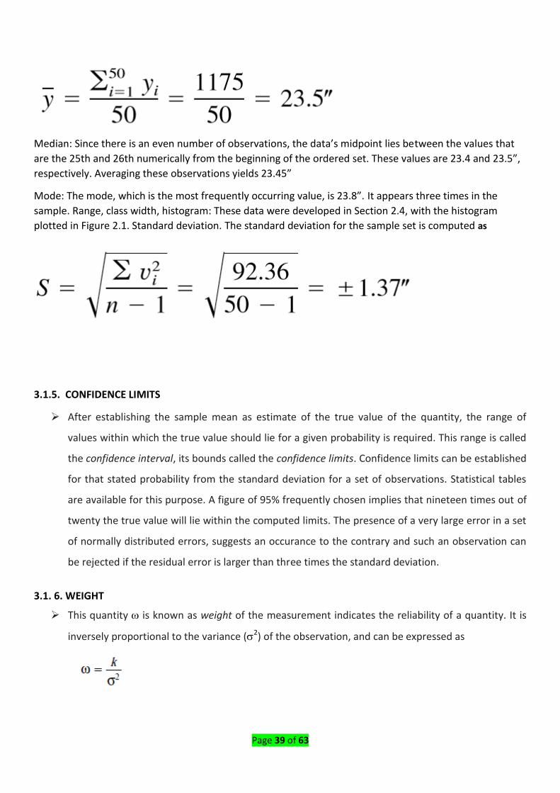
Page 39 of 63
Median: Since there is an even number of observations, the data’s midpoint lies between the values that
are the 25th and 26th numerically from the beginning of the ordered set. These values are 23.4 and 23.5”,
respectively. Averaging these observations yields 23.45”
Mode: The mode, which is the most frequently occurring value, is 23.8”. It appears three times in the
sample. Range, class width, histogram: These data were developed in Section 2.4, with the histogram
plotted in Figure 2.1. Standard deviation. The standard deviation for the sample set is computed as
3.1.5. CONFIDENCE LIMITS
After establishing the sample mean as estimate of the true value of the quantity, the range of
values within which the true value should lie for a given probability is required. This range is called
the confidence interval, its bounds called the confidence limits. Confidence limits can be established
for that stated probability from the standard deviation for a set of observations. Statistical tables
are available for this purpose. A figure of 95% frequently chosen implies that nineteen times out of
twenty the true value will lie within the computed limits. The presence of a very large error in a set
of normally distributed errors, suggests an occurance to the contrary and such an observation can
be rejected if the residual error is larger than three times the standard deviation.
3.1. 6. WEIGHT
This quantity is known as weight of the measurement indicates the reliability of a quantity. It is
inversely proportional to the variance (2) of the observation, and can be expressed as

Page 40 of 63
Where k is a constant of proportionality. If the weights and the standard errors for observations x1,
x2, ,….., etc., are respectively 1 , 2 ω ,….., etc., and 1 , 2 ,….., etc., and u is the standard error
for the observation having unit weight then we have
The weights are applied to the individual measurements of unequal reliability to reduce them to one
standard. The most probable value is then the weighted mean xm of the measurements. Thus
and standard error of the wieghted mean
The standard deviation of an observation of unit weight is given by
and the standard deviation of an observation of weight n is given by
3.1.7. PROPAGATION OF ERROR
The calculation of quantities such as areas, volumes, difference in height, horizontal distance, etc., using
the measured quantities distances and angles, is done through mathematical relationships between the
computed quantities and the measured quantities. Since the measured quantities have errors, it is

Page 41 of 63
inevitable that the quantities computed from them will not have errors. Evaluation of the errors in the
computed quantities as the function of errors in the measurements is called error propagation.
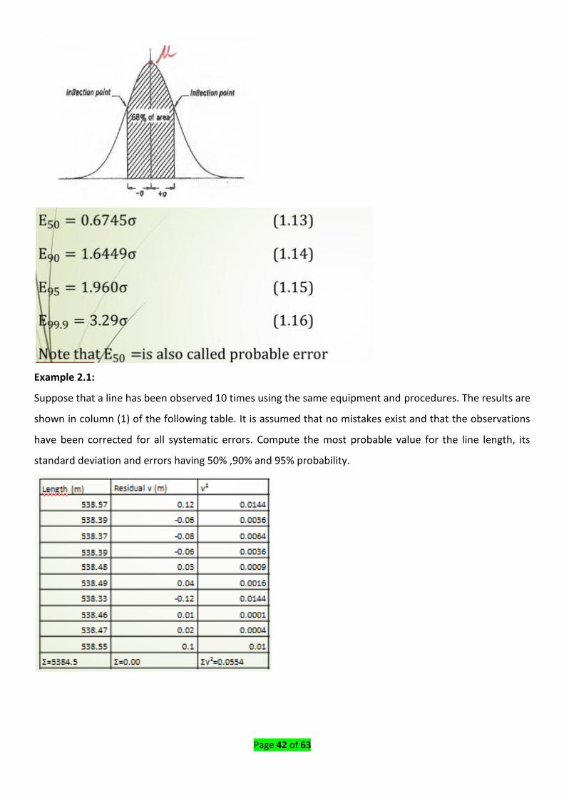
3.1.8. Normal Distribution
Measured quantities in surveying (angles, distances,…) and in many surveying domain are random
variables that obey normal distribution. The corresponding probability density is:
being the true value of the measured quantity, the error of measurements equals:
=x-
In that manner, the probability density can be written as:
This is the probability density to make an error of measurements.
To that of making an error comprises between and 1
Particular case: P (-
Can be written as = i.e the probability to make an error of equals 0.68 or68%.
Page 42 of 63
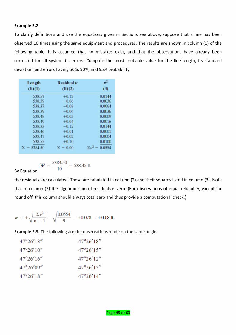
Example 2.1:
Suppose that a line has been observed 10 times using the same equipment and procedures. The results are
shown in column (1) of the following table. It is assumed that no mistakes exist and that the observations
have been corrected for all systematic errors. Compute the most probable value for the line length, its
standard deviation and errors having 50% ,90% and 95% probability.

Page 43 of 63

Page 44 of 63
Page 45 of 63
Example 2.2
To clarify definitions and use the equations given in Sections see above, suppose that a line has been
observed 10 times using the same equipment and procedures. The results are shown in column (1) of the
following table. It is assumed that no mistakes exist, and that the observations have already been
corrected for all systematic errors. Compute the most probable value for the line length, its standard
deviation, and errors having 50%, 90%, and 95% probability
By Equation
the residuals are calculated. These are tabulated in column (2) and their squares listed in column (3). Note
that in column (2) the algebraic sum of residuals is zero. (For observations of equal reliability, except for
round off, this column should always total zero and thus provide a computational check.)
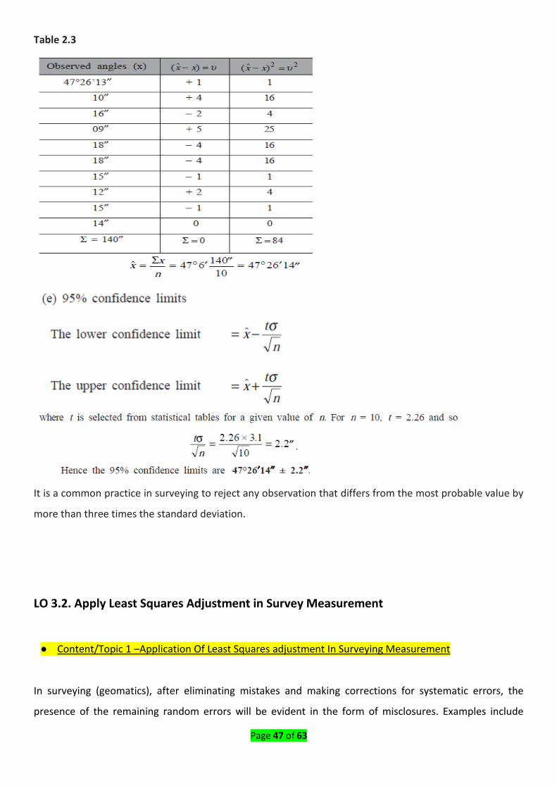
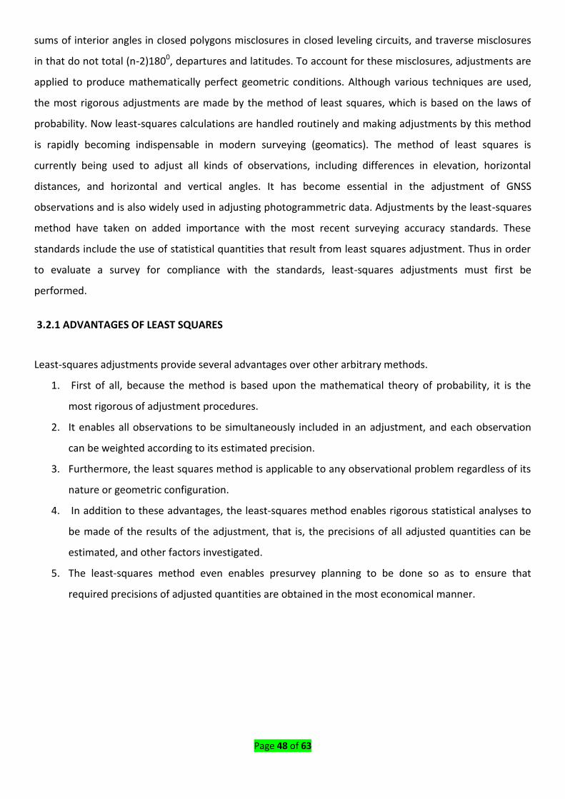
Example 2.3. The following are the observations made on the same angle:

Page 46 of 63
Determine
(a) the most probable value of the angle,
(b) The range,
(c) The standard deviation,
(d) The standard error of the mean, and
(e) The 95% confidence limits.
Solution:
For convenience in calculation of the required quantities let us tabulate the data as in Table 2.3.
The total number of observations n = 10.
Page 47 of 63
Table 2.3
It is a common practice in surveying to reject any observation that differs from the most probable value by
more than three times the standard deviation.
LO 3.2. Apply Least Squares Adjustment in Survey Measurement
● Content/Topic 1 –Application Of Least Squares adjustment In Surveying Measurement
In surveying (geomatics), after eliminating mistakes and making corrections for systematic errors, the
presence of the remaining random errors will be evident in the form of misclosures. Examples include
Page 48 of 63
sums of interior angles in closed polygons misclosures in closed leveling circuits, and traverse misclosures
in that do not total (n-2)1800, departures and latitudes. To account for these misclosures, adjustments are
applied to produce mathematically perfect geometric conditions. Although various techniques are used,
the most rigorous adjustments are made by the method of least squares, which is based on the laws of
probability. Now least-squares calculations are handled routinely and making adjustments by this method
is rapidly becoming indispensable in modern surveying (geomatics). The method of least squares is
currently being used to adjust all kinds of observations, including differences in elevation, horizontal
distances, and horizontal and vertical angles. It has become essential in the adjustment of GNSS
observations and is also widely used in adjusting photogrammetric data. Adjustments by the least-squares
method have taken on added importance with the most recent surveying accuracy standards. These
standards include the use of statistical quantities that result from least squares adjustment. Thus in order
to evaluate a survey for compliance with the standards, least-squares adjustments must first be
performed.
3.2.1 ADVANTAGES OF LEAST SQUARES
Least-squares adjustments provide several advantages over other arbitrary methods.
1. First of all, because the method is based upon the mathematical theory of probability, it is the
most rigorous of adjustment procedures.
2. It enables all observations to be simultaneously included in an adjustment, and each observation
can be weighted according to its estimated precision.
3. Furthermore, the least squares method is applicable to any observational problem regardless of its
nature or geometric configuration.
4. In addition to these advantages, the least-squares method enables rigorous statistical analyses to
be made of the results of the adjustment, that is, the precisions of all adjusted quantities can be
estimated, and other factors investigated.
5. The least-squares method even enables presurvey planning to be done so as to ensure that
required precisions of adjusted quantities are obtained in the most economical manner.
Page 49 of 63
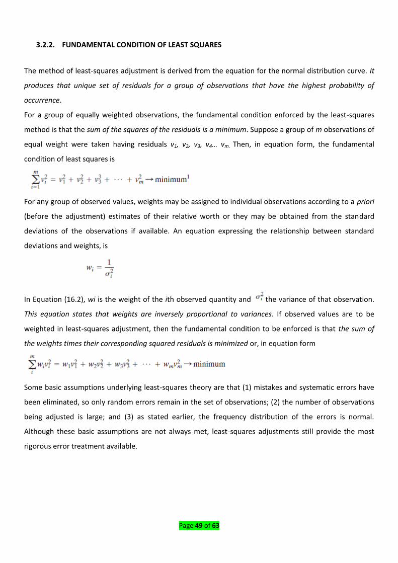
3.2.2. FUNDAMENTAL CONDITION OF LEAST SQUARES
The method of least-squares adjustment is derived from the equation for the normal distribution curve. It
produces that unique set of residuals for a group of observations that have the highest probability of
occurrence.
For a group of equally weighted observations, the fundamental condition enforced by the least-squares
method is that the sum of the squares of the residuals is a minimum. Suppose a group of m observations of
equal weight were taken having residuals v1, v2, v3, v4… vm. Then, in equation form, the fundamental
condition of least squares is
For any group of observed values, weights may be assigned to individual observations according to a priori
(before the adjustment) estimates of their relative worth or they may be obtained from the standard
deviations of the observations if available. An equation expressing the relationship between standard
deviations and weights, is
In Equation (16.2), wi is the weight of the ith observed quantity and the variance of that observation.
This equation states that weights are inversely proportional to variances. If observed values are to be
weighted in least-squares adjustment, then the fundamental condition to be enforced is that the sum of
the weights times their corresponding squared residuals is minimized or, in equation form
Some basic assumptions underlying least-squares theory are that (1) mistakes and systematic errors have
been eliminated, so only random errors remain in the set of observations; (2) the number of observations
being adjusted is large; and (3) as stated earlier, the frequency distribution of the errors is normal.
Although these basic assumptions are not always met, least-squares adjustments still provide the most
rigorous error treatment available.
Page 50 of 63
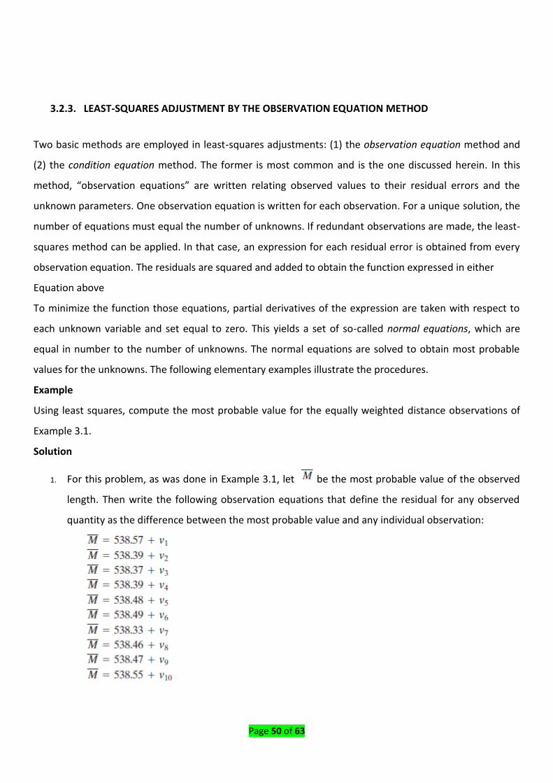
3.2.3. LEAST-SQUARES ADJUSTMENT BY THE OBSERVATION EQUATION METHOD
Two basic methods are employed in least-squares adjustments: (1) the observation equation method and
(2) the condition equation method. The former is most common and is the one discussed herein. In this
method, “observation equations” are written relating observed values to their residual errors and the
unknown parameters. One observation equation is written for each observation. For a unique solution, the
number of equations must equal the number of unknowns. If redundant observations are made, the least-
squares method can be applied. In that case, an expression for each residual error is obtained from every
observation equation. The residuals are squared and added to obtain the function expressed in either
Equation above
To minimize the function those equations, partial derivatives of the expression are taken with respect to
each unknown variable and set equal to zero. This yields a set of so-called normal equations, which are
equal in number to the number of unknowns. The normal equations are solved to obtain most probable
values for the unknowns. The following elementary examples illustrate the procedures.
Example
Using least squares, compute the most probable value for the equally weighted distance observations of
Example 3.1.
Solution
1. For this problem, as was done in Example 3.1, let be the most probable value of the observed
length. Then write the following observation equations that define the residual for any observed
quantity as the difference between the most probable value and any individual observation:
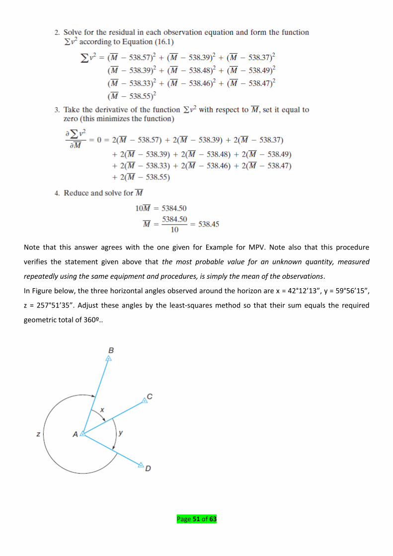
Page 51 of 63
Note that this answer agrees with the one given for Example for MPV. Note also that this procedure
verifies the statement given above that the most probable value for an unknown quantity, measured
repeatedly using the same equipment and procedures, is simply the mean of the observations.
In Figure below, the three horizontal angles observed around the horizon are x = 42°12’13”, y = 59°56’15”,
z = 257°51’35”. Adjust these angles by the least-squares method so that their sum equals the required
geometric total of 360º..
Page 52 of 63
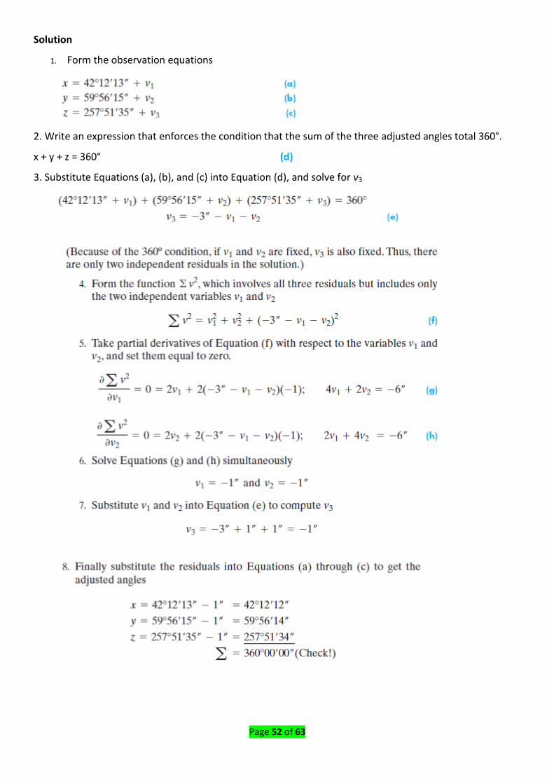
Solution
1. Form the observation equations
2. Write an expression that enforces the condition that the sum of the three adjusted angles total 360°.
x + y + z = 360° (d)
3. Substitute Equations (a), (b), and (c) into Equation (d), and solve for v3

Page 53 of 63
Example 16.3
Adjust the three equally weighted distance observations taken (in feet) between points A, B, and C of
Figure below.
Solution
1. Let the unknown distances AB and BC be x and y, respectively. These two unknowns are related through
the observations as follows:
x + y = 393.65
x = 190.40
y = 203.16
2. Values for x and y could be obtained from any two of these equations so that the remaining equation is
redundant. However, notice that values
Page 54 of 63
2.5.4 MATRIX METHODS IN LEAST-SQUARES ADJUSTMENT
It has been noted that least-squares computations are quite lengthy, and therefore generally performed on
a computer. Their solution follows a systematic procedure hat is conveniently adapted to matrix methods.
In general, any group of observation equations may be represented in matrix form as
Where A is the matrix of coefficients for the unknowns, X the matrix of unknowns, L the matrix of
observations, and V the matrix of residuals. The detailed structures of these matrices are
The normal equations that result from a set of equally weighted observation equations are given in matrix
form by

Page 55 of 63
In Equations AT A is the matrix of normal equation coefficients for the unknowns. Premultiplying both sides
of Equation (AT A)-1 by and reducing yields
Equation (16.6) is the least-squares solution for equally weighted observations. The matrix X consists of
most probable values for unknowns for a system of weighted observations, the
following equation provides the X matrix:
In Equation (16.7) the matrices are identical to those of the equally weighted case, except that W is a
diagonal matrix of weights defined as follows
Solve Example 16.3 using matrix methods.
Page 56 of 63
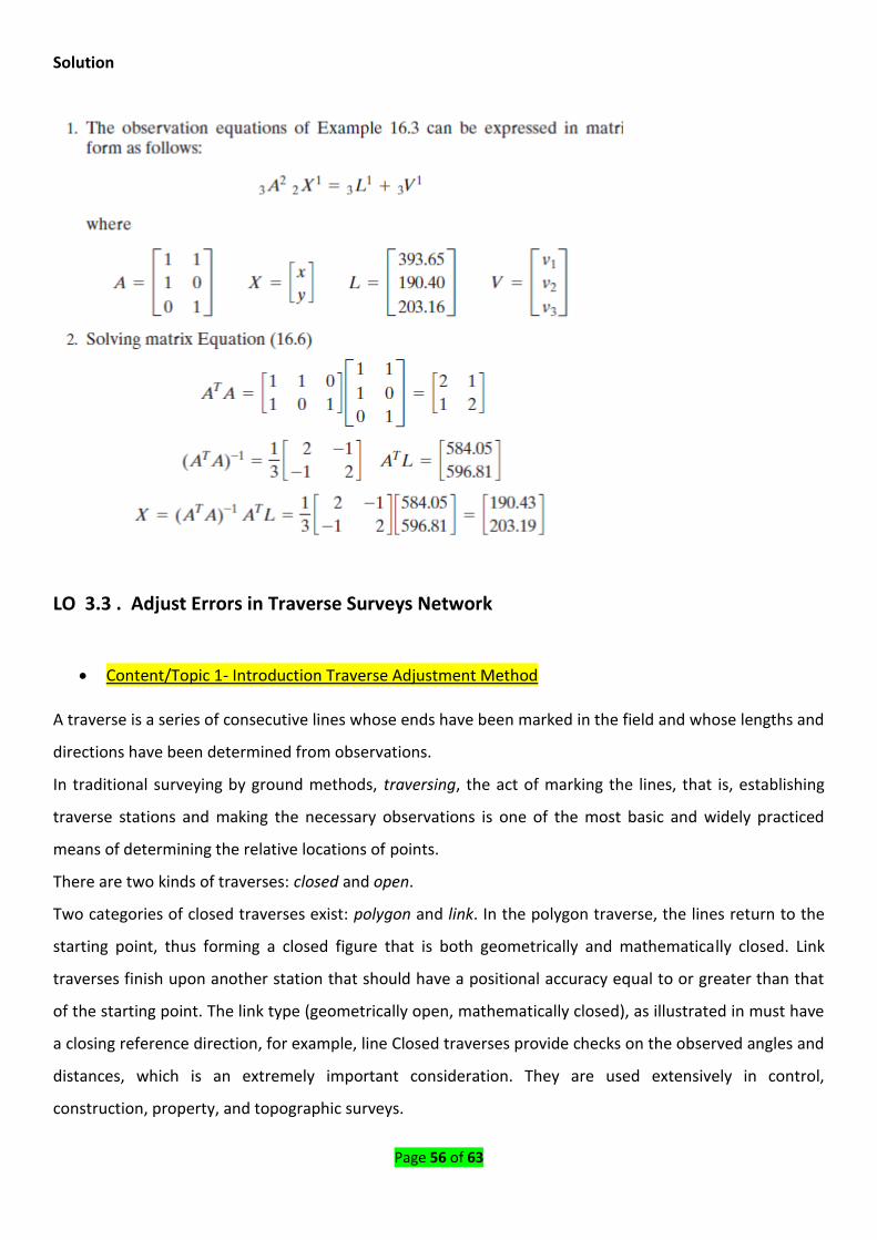
Solution
LO 3.3 . Adjust Errors in Traverse Surveys Network
Content/Topic 1- Introduction Traverse Adjustment Method
A traverse is a series of consecutive lines whose ends have been marked in the field and whose lengths and
directions have been determined from observations.
In traditional surveying by ground methods, traversing, the act of marking the lines, that is, establishing
traverse stations and making the necessary observations is one of the most basic and widely practiced
means of determining the relative locations of points.
There are two kinds of traverses: closed and open.
Two categories of closed traverses exist: polygon and link. In the polygon traverse, the lines return to the
starting point, thus forming a closed figure that is both geometrically and mathematically closed. Link
traverses finish upon another station that should have a positional accuracy equal to or greater than that
of the starting point. The link type (geometrically open, mathematically closed), as illustrated in must have
a closing reference direction, for example, line Closed traverses provide checks on the observed angles and
distances, which is an extremely important consideration. They are used extensively in control,
construction, property, and topographic surveys.
Page 57 of 63
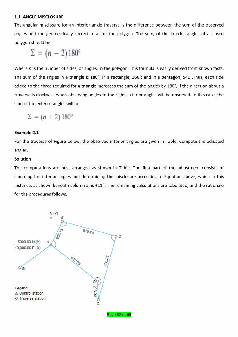
1.1. ANGLE MISCLOSURE
The angular misclosure for an interior-angle traverse is the difference between the sum of the observed
angles and the geometrically correct total for the polygon. The sum, of the interior angles of a closed
polygon should be
Where n is the number of sides, or angles, in the polygon. This formula is easily derived from known facts.
The sum of the angles in a triangle is 180°; in a rectangle, 360°; and in a pentagon, 540°.Thus, each side
added to the three required for a triangle increases the sum of the angles by 180°, if the direction about a
traverse is clockwise when observing angles to the right, exterior angles will be observed. In this case, the
sum of the exterior angles will be
Example 2.1
For the traverse of Figure below, the observed interior angles are given in Table. Compute the adjusted
angles.
Solution
The computations are best arranged as shown in Table. The first part of the adjustment consists of
summing the interior angles and determining the misclosure according to Equation above, which in this
instance, as shown beneath column 2, is +11”. The remaining calculations are tabulated, and the rationale
for the procedures follows.
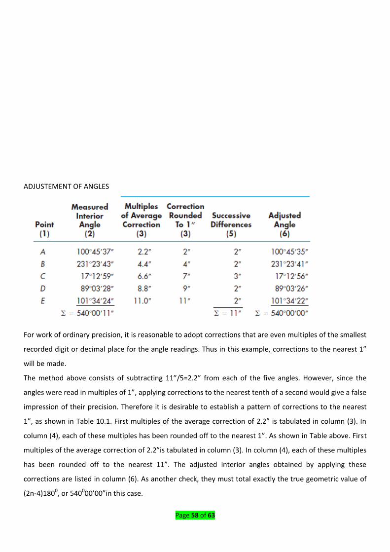
Page 58 of 63
ADJUSTEMENT OF ANGLES
For work of ordinary precision, it is reasonable to adopt corrections that are even multiples of the smallest
recorded digit or decimal place for the angle readings. Thus in this example, corrections to the nearest 1”
will be made.
The method above consists of subtracting 11”/5=2.2” from each of the five angles. However, since the
angles were read in multiples of 1”, applying corrections to the nearest tenth of a second would give a false
impression of their precision. Therefore it is desirable to establish a pattern of corrections to the nearest
1”, as shown in Table 10.1. First multiples of the average correction of 2.2” is tabulated in column (3). In
column (4), each of these multiples has been rounded off to the nearest 1”. As shown in Table above. First
multiples of the average correction of 2.2”is tabulated in column (3). In column (4), each of these multiples
has been rounded off to the nearest 11”. The adjusted interior angles obtained by applying these
corrections are listed in column (6). As another check, they must total exactly the true geometric value of
(2n-4)1800, or 540000’00”in this case.
Page 59 of 63
1.2 COMPUTATION OF PRELIMINARY AZIMUTHS OR BEARINGS
If a line of known direction exists within the traverse, computation of preliminary azimuths (or bearings)
proceeds as discussed in Chapter 7. Angles adjusted to the
proper geometric total must be used; otherwise the azimuth or bearing of the first line, when recomputed
after using all angles and progressing around the traverse, will differ from its fixed value by the angular
misclosure.
Azimuths or bearings at this stage are called “preliminary” because they will change after the traverse is
adjusted, as explained in Section 10.11. It should also be noted that since the azimuth of the courses will
change, so will the angles, which were previously adjusted. Briefly by the equation
Example 2.2
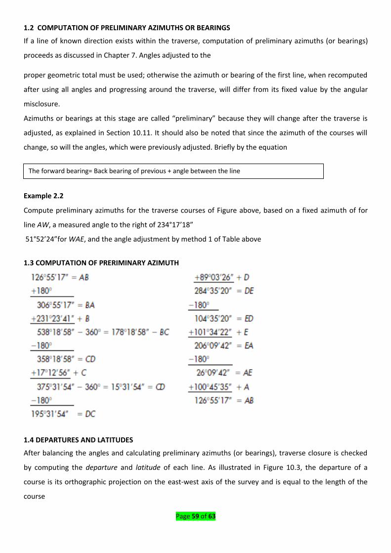
Compute preliminary azimuths for the traverse courses of Figure above, based on a fixed azimuth of for
line AW, a measured angle to the right of 234°17’18”
51°52’24”for WAE, and the angle adjustment by method 1 of Table above
1.3 COMPUTATION OF PRERIMINARY AZIMUTH
1.4 DEPARTURES AND LATITUDES
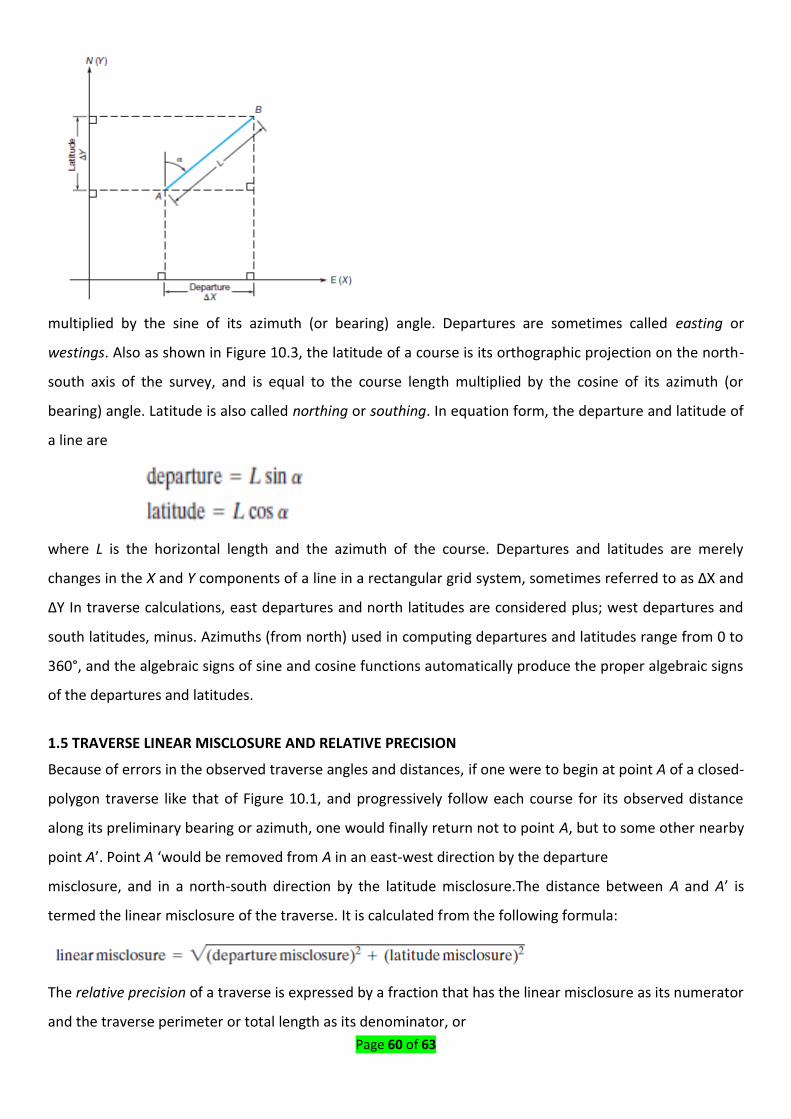
After balancing the angles and calculating preliminary azimuths (or bearings), traverse closure is checked
by computing the departure and latitude of each line. As illustrated in Figure 10.3, the departure of a
course is its orthographic projection on the east-west axis of the survey and is equal to the length of the
course
The forward bearing= Back bearing of previous + angle between the line
Page 60 of 63
multiplied by the sine of its azimuth (or bearing) angle. Departures are sometimes called easting or
westings. Also as shown in Figure 10.3, the latitude of a course is its orthographic projection on the north-
south axis of the survey, and is equal to the course length multiplied by the cosine of its azimuth (or
bearing) angle. Latitude is also called northing or southing. In equation form, the departure and latitude of
a line are
where L is the horizontal length and the azimuth of the course. Departures and latitudes are merely
changes in the X and Y components of a line in a rectangular grid system, sometimes referred to as ΔX and
ΔY In traverse calculations, east departures and north latitudes are considered plus; west departures and
south latitudes, minus. Azimuths (from north) used in computing departures and latitudes range from 0 to
360°, and the algebraic signs of sine and cosine functions automatically produce the proper algebraic signs
of the departures and latitudes.
1.5 TRAVERSE LINEAR MISCLOSURE AND RELATIVE PRECISION
Because of errors in the observed traverse angles and distances, if one were to begin at point A of a closed-
polygon traverse like that of Figure 10.1, and progressively follow each course for its observed distance
along its preliminary bearing or azimuth, one would finally return not to point A, but to some other nearby
point A’. Point A ‘would be removed from A in an east-west direction by the departure
misclosure, and in a north-south direction by the latitude misclosure.The distance between A and A’ is
termed the linear misclosure of the traverse. It is calculated from the following formula:
The relative precision of a traverse is expressed by a fraction that has the linear misclosure as its numerator
and the traverse perimeter or total length as its denominator, or
Page 61 of 63
The fraction that results from Equation (10.4) is then reduced to reciprocal form, and the denominator
rounded to the same number of significant figures as the numerator.This is illustrated in the following
example.
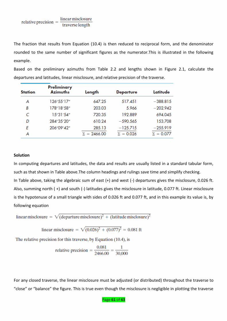
Based on the preliminary azimuths from Table 2.2 and lengths shown in Figure 2.1, calculate the
departures and latitudes, linear misclosure, and relative precision of the traverse.
Solution
In computing departures and latitudes, the data and results are usually listed in a standard tabular form,
such as that shown in Table above.The column headings and rulings save time and simplify checking.
In Table above, taking the algebraic sum of east (+) and west (-) departures gives the misclosure, 0.026 ft.
Also, summing north ( +) and south (-) latitudes gives the misclosure in latitude, 0.077 ft. Linear misclosure
is the hypotenuse of a small triangle with sides of 0.026 ft and 0.077 ft, and in this example its value is, by
following equation
For any closed traverse, the linear misclosure must be adjusted (or distributed) throughout the traverse to
“close” or “balance” the figure. This is true even though the misclosure is negligible in plotting the traverse

Page 62 of 63
at map scale. There are several elementary methods available for traverse adjustment, but the one most
commonly used is the compass rule (Bowditch method). As noted earlier, adjustment by least squares is a
more advanced technique that can also be used. These two methods are discussed in the subsections that
follow.
Page 63 of 63
REFERENCES
1. W. Schofield, M. Breach, Engineering surveying 6th edition, Kingston University,2007
2. CHARLES D. GHILANI, PAUL R. WOLF, Elementary surveying 13th edition, Pennsylvania State 2012
3. Basic surveying -theory and practice, Oregon Department of Transportation Geometronics Unit,
Bend, Oregon 2000
4. Kanetkar, T. P., and Kulkarni, S. V. 1981. Surveying and Leveling, Vol I. Pune Vidyarthi Griha Praksam
, Pune.
5. Murthy, V. V. N. 1982. Land and Water Management Engineering. Kalyani publishers, New Delhi.
6. Michael, A. M. 1989. Irrigation Theory and Practice. Vikas Publishing House Pvt. Ltd, New Delhi.
7. Michael, A. M., and Ojha, T. P. 1993. Principles of Agricultural Engineering – Vol. II. Jain Brothers,
New Delhi.
8. Mal, B. C. 2005. Introduction to Soil and Water Conservation Engineering. Kalyani publishers, New
Delhi.
9. Dr A M Chandra. 2005. Problem solving with theory and objective type question New Delhi'
Bangalore ' Chennai