credit risk modeling - stephane papastephanakis · 2016-03-06 · credit risk modeling math 587:...
TRANSCRIPT

CREDIT RISK MODELING
MATH 587: Course Notes
Tomasz R. BieleckiDepartment of Applied Mathematics
Illinois Institute of TechnologyChicago, IL 60616, USA
Monique JeanblancDepartement de Mathematiques
Universite d’Evry Val d’Essonne
91025 Evry Cedex, France
Marek RutkowskiSchool of Mathematics and Statistics
University of New South WalesSydney, NSW 2052, Australia
Applied Mathematics DepartmentIllinois Institute of Technology
Fall 2008

2

Contents
1 Structural Approach 9
1.1 Basic Assumptions . . . . . . . . . . . . . . . . . . . . . . . . . . . . . . . . . . . . . 9
1.1.1 Defaultable Claims . . . . . . . . . . . . . . . . . . . . . . . . . . . . . . . . . 9
1.1.2 Risk-Neutral Valuation Formula . . . . . . . . . . . . . . . . . . . . . . . . . 10
1.1.3 Defaultable Zero-Coupon Bond . . . . . . . . . . . . . . . . . . . . . . . . . . 11
1.2 Merton’s Model of a Corporate Debt . . . . . . . . . . . . . . . . . . . . . . . . . . . 12
1.3 Properties of First Passage Times . . . . . . . . . . . . . . . . . . . . . . . . . . . . . 14
1.3.1 Probability Law of the First Passage Time . . . . . . . . . . . . . . . . . . . 15
1.3.2 Joint Probability Law of Y and τ . . . . . . . . . . . . . . . . . . . . . . . . . 17
1.4 Black and Cox Model . . . . . . . . . . . . . . . . . . . . . . . . . . . . . . . . . . . 21
1.4.1 Black and Cox Formula . . . . . . . . . . . . . . . . . . . . . . . . . . . . . . 22
1.4.2 Corporate Coupon Bond . . . . . . . . . . . . . . . . . . . . . . . . . . . . . . 26
1.4.3 Optimal Capital Structure . . . . . . . . . . . . . . . . . . . . . . . . . . . . . 28
1.5 Extensions of the Black and Cox Model . . . . . . . . . . . . . . . . . . . . . . . . . 29
1.5.1 Stochastic Interest Rates . . . . . . . . . . . . . . . . . . . . . . . . . . . . . 30
1.6 Random Barrier . . . . . . . . . . . . . . . . . . . . . . . . . . . . . . . . . . . . . . 31
1.6.1 Independent Barrier . . . . . . . . . . . . . . . . . . . . . . . . . . . . . . . . 32
2 Hazard Function Approach 33
2.1 Elementary Market Model . . . . . . . . . . . . . . . . . . . . . . . . . . . . . . . . . 33
2.1.1 Hazard Function . . . . . . . . . . . . . . . . . . . . . . . . . . . . . . . . . . 33
2.1.2 Defaultable Zero-Coupon Bond with Recovery at Maturity . . . . . . . . . . 34
2.1.3 Defaultable Zero-Coupon with Recovery at Default . . . . . . . . . . . . . . . 37
2.2 Martingale Approach . . . . . . . . . . . . . . . . . . . . . . . . . . . . . . . . . . . . 38
2.2.1 Conditional Expectations . . . . . . . . . . . . . . . . . . . . . . . . . . . . . 39
2.2.2 Martingales Associated with Default Time . . . . . . . . . . . . . . . . . . . . 39
2.2.3 Predictable Representation Theorem . . . . . . . . . . . . . . . . . . . . . . . 43
2.2.4 Girsanov’s Theorem . . . . . . . . . . . . . . . . . . . . . . . . . . . . . . . . 45
2.2.5 Range of Arbitrage Prices . . . . . . . . . . . . . . . . . . . . . . . . . . . . . 47
2.2.6 Implied Risk-Neutral Default Intensity . . . . . . . . . . . . . . . . . . . . . . 48
2.2.7 Dynamics of Prices of Defaultable Claims . . . . . . . . . . . . . . . . . . . . 49
2.3 Generic Defaultable Claims . . . . . . . . . . . . . . . . . . . . . . . . . . . . . . . . 50
3

4 CONTENTS
2.3.1 Buy-and-Hold Strategy . . . . . . . . . . . . . . . . . . . . . . . . . . . . . . 51
2.3.2 Spot Martingale Measure . . . . . . . . . . . . . . . . . . . . . . . . . . . . . 53
2.3.3 Self-Financing Trading Strategies . . . . . . . . . . . . . . . . . . . . . . . . . 54
2.3.4 Martingale Properties of Prices of Defaultable Claims . . . . . . . . . . . . . 56
2.4 Hedging of Single Name Credit Derivatives . . . . . . . . . . . . . . . . . . . . . . . 56
2.4.1 Stylized Credit Default Swap . . . . . . . . . . . . . . . . . . . . . . . . . . . 56
2.4.2 Pricing of a CDS . . . . . . . . . . . . . . . . . . . . . . . . . . . . . . . . . . 57
2.4.3 Market CDS Rate . . . . . . . . . . . . . . . . . . . . . . . . . . . . . . . . . 58
2.4.4 Price Dynamics of a CDS . . . . . . . . . . . . . . . . . . . . . . . . . . . . . 59
2.4.5 Dynamic Replication of a Defaultable Claim . . . . . . . . . . . . . . . . . . 60
2.5 Dynamic Hedging of Basket Credit Derivatives . . . . . . . . . . . . . . . . . . . . . 62
2.5.1 First-to-Default Intensities . . . . . . . . . . . . . . . . . . . . . . . . . . . . 63
2.5.2 First-to-Default Martingale Representation Theorem . . . . . . . . . . . . . . 64
2.5.3 Price Dynamics of the ith CDS . . . . . . . . . . . . . . . . . . . . . . . . . . 66
2.5.4 Risk-Neutral Valuation of a First-to-Default Claim . . . . . . . . . . . . . . . 68
2.5.5 Dynamic Replication of a First-to-Default Claim . . . . . . . . . . . . . . . . 69
2.5.6 Conditional Default Distributions . . . . . . . . . . . . . . . . . . . . . . . . . 71
2.5.7 Recursive Valuation of a Basket Claim . . . . . . . . . . . . . . . . . . . . . . 72
2.5.8 Recursive Replication of a Basket Claim . . . . . . . . . . . . . . . . . . . . . 75
2.6 Applications to Copula-Based Credit Risk Models . . . . . . . . . . . . . . . . . . . 75
2.6.1 Independent Default Times . . . . . . . . . . . . . . . . . . . . . . . . . . . . 76
2.6.2 Archimedean Copulas . . . . . . . . . . . . . . . . . . . . . . . . . . . . . . . 77
3 Hazard Process Approach 81
3.1 Hazard Process and its Applications . . . . . . . . . . . . . . . . . . . . . . . . . . . 81
3.1.1 Conditional Expectations . . . . . . . . . . . . . . . . . . . . . . . . . . . . . 82
3.1.2 Stochastic Intensity . . . . . . . . . . . . . . . . . . . . . . . . . . . . . . . . 84
3.1.3 Valuation of Defaultable Claims . . . . . . . . . . . . . . . . . . . . . . . . . 84
3.1.4 Martingales Associated with Default Time . . . . . . . . . . . . . . . . . . . . 86
3.1.5 Reduction of the Reference Filtration . . . . . . . . . . . . . . . . . . . . . . 88
3.1.6 Enlargement of Filtration . . . . . . . . . . . . . . . . . . . . . . . . . . . . . 90
3.2 Hypothesis (H) . . . . . . . . . . . . . . . . . . . . . . . . . . . . . . . . . . . . . . . 90
3.2.1 Equivalent Formulations . . . . . . . . . . . . . . . . . . . . . . . . . . . . . . 90
3.2.2 Canonical Construction of a Default Time . . . . . . . . . . . . . . . . . . . . 92
3.2.3 Stochastic Barrier . . . . . . . . . . . . . . . . . . . . . . . . . . . . . . . . . 92
3.3 Predictable Representation Theorem . . . . . . . . . . . . . . . . . . . . . . . . . . . 93
3.4 Girsanov’s Theorem . . . . . . . . . . . . . . . . . . . . . . . . . . . . . . . . . . . . 94
3.5 Invariance of Hypothesis (H) . . . . . . . . . . . . . . . . . . . . . . . . . . . . . . . 96
3.5.1 Case of the Brownian Filtration . . . . . . . . . . . . . . . . . . . . . . . . . . 97
3.5.2 Extension to Orthogonal Martingales . . . . . . . . . . . . . . . . . . . . . . . 98
3.6 Alternative Approach . . . . . . . . . . . . . . . . . . . . . . . . . . . . . . . . . . . 100

CONTENTS 5
3.7 Single-Name Credit Default Swap Market . . . . . . . . . . . . . . . . . . . . . . . . 101
3.7.1 Price Dynamics in a Single-Name Model . . . . . . . . . . . . . . . . . . . . . 101
3.7.2 Replication of a Defaultable Claim . . . . . . . . . . . . . . . . . . . . . . . . 109
3.8 Multi-Name Credit Default Swap Market . . . . . . . . . . . . . . . . . . . . . . . . 116
3.8.1 Price Dynamics in a Multi-Name Model . . . . . . . . . . . . . . . . . . . . . 116
3.8.2 Replication of a First-to-Default Claim . . . . . . . . . . . . . . . . . . . . . . 121
4 Hedging of Defaultable Claims 123
4.1 Semimartingale Model with a Common Default . . . . . . . . . . . . . . . . . . . . . 123
4.1.1 Dynamics of Asset Prices . . . . . . . . . . . . . . . . . . . . . . . . . . . . . 123
4.2 Trading Strategies in a Semimartingale Set-up . . . . . . . . . . . . . . . . . . . . . 126
4.2.1 Unconstrained Strategies . . . . . . . . . . . . . . . . . . . . . . . . . . . . . 126
4.2.2 Constrained Strategies . . . . . . . . . . . . . . . . . . . . . . . . . . . . . . . 128
4.3 Martingale Approach to Valuation and Hedging . . . . . . . . . . . . . . . . . . . . . 132
4.3.1 Defaultable Asset with Total Default . . . . . . . . . . . . . . . . . . . . . . . 132
4.3.2 Defaultable Asset with Non-Zero Recovery . . . . . . . . . . . . . . . . . . . 144
4.3.3 Two Defaultable Assets with Total Default . . . . . . . . . . . . . . . . . . . 145
4.4 PDE Approach to Valuation and Hedging . . . . . . . . . . . . . . . . . . . . . . . . 148
4.4.1 Defaultable Asset with Total Default . . . . . . . . . . . . . . . . . . . . . . . 148
4.4.2 Defaultable Asset with Non-Zero Recovery . . . . . . . . . . . . . . . . . . . 152
4.4.3 Two Defaultable Assets with Total Default . . . . . . . . . . . . . . . . . . . 155
5 Dependent Defaults and Credit Migrations 157
5.1 Basket Credit Derivatives . . . . . . . . . . . . . . . . . . . . . . . . . . . . . . . . . 158
5.1.1 The ith-to-Default Contingent Claims . . . . . . . . . . . . . . . . . . . . . . 158
5.1.2 Case of Two Entities . . . . . . . . . . . . . . . . . . . . . . . . . . . . . . . . 158
5.1.3 Role of the Hypothesis (H) . . . . . . . . . . . . . . . . . . . . . . . . . . . . 159
5.2 Conditionally Independent Defaults . . . . . . . . . . . . . . . . . . . . . . . . . . . . 159
5.2.1 Canonical Construction . . . . . . . . . . . . . . . . . . . . . . . . . . . . . . 160
5.2.2 Independent Default Times . . . . . . . . . . . . . . . . . . . . . . . . . . . . 160
5.2.3 Signed Intensities . . . . . . . . . . . . . . . . . . . . . . . . . . . . . . . . . . 161
5.2.4 Valuation of FTDC and LTDC . . . . . . . . . . . . . . . . . . . . . . . . . . 162
5.3 Copula-Based Approaches . . . . . . . . . . . . . . . . . . . . . . . . . . . . . . . . . 163
5.3.1 Direct Approach . . . . . . . . . . . . . . . . . . . . . . . . . . . . . . . . . . 163
5.3.2 Indirect Approach . . . . . . . . . . . . . . . . . . . . . . . . . . . . . . . . . 163
5.4 Jarrow and Yu Model . . . . . . . . . . . . . . . . . . . . . . . . . . . . . . . . . . . 165
5.4.1 Construction and Properties of the Model . . . . . . . . . . . . . . . . . . . . 165
5.5 Extension of the Jarrow and Yu Model . . . . . . . . . . . . . . . . . . . . . . . . . . 169
5.5.1 Kusuoka’s Construction . . . . . . . . . . . . . . . . . . . . . . . . . . . . . . 169
5.5.2 Bond Valuation . . . . . . . . . . . . . . . . . . . . . . . . . . . . . . . . . . . 170
5.6 Markovian Models of Credit Migrations . . . . . . . . . . . . . . . . . . . . . . . . . 171

6 CONTENTS
5.6.1 Infinitesimal Generator . . . . . . . . . . . . . . . . . . . . . . . . . . . . . . 171
5.6.2 Specification of Credit Ratings Transition Intensities . . . . . . . . . . . . . . 173
5.6.3 Conditionally Independent Migrations . . . . . . . . . . . . . . . . . . . . . . 174
5.6.4 Examples of Markov Market Models . . . . . . . . . . . . . . . . . . . . . . . 174
5.6.5 Forward CDS . . . . . . . . . . . . . . . . . . . . . . . . . . . . . . . . . . . . 176
5.6.6 Credit Default Swaptions . . . . . . . . . . . . . . . . . . . . . . . . . . . . . 176
5.7 Basket Credit Derivatives . . . . . . . . . . . . . . . . . . . . . . . . . . . . . . . . . 177
5.7.1 kth-to-Default CDS . . . . . . . . . . . . . . . . . . . . . . . . . . . . . . . . . 178
5.7.2 Forward kth-to-Default CDS . . . . . . . . . . . . . . . . . . . . . . . . . . . 179
5.7.3 Model Implementation . . . . . . . . . . . . . . . . . . . . . . . . . . . . . . . 180
5.7.4 Standard Credit Basket Products . . . . . . . . . . . . . . . . . . . . . . . . . 183
5.7.5 Valuation of Standard Basket Credit Derivatives . . . . . . . . . . . . . . . . 186
6 Appendix: Conditional Poisson Process 189
6.1 Poisson Process with Constant Intensity . . . . . . . . . . . . . . . . . . . . . . . . . 189
6.2 Poisson Process with Deterministic Intensity . . . . . . . . . . . . . . . . . . . . . . 194
6.3 Conditional Poisson Process . . . . . . . . . . . . . . . . . . . . . . . . . . . . . . . . 195

Introduction
The goal of these lecture notes is to present a survey of some recent developments in the areaof mathematical modeling of credit risk. They are largely based on the following papers by T.R.Bielecki, M. Jeanblanc and M. Rutkowski:
• Modelling and valuation of credit risk. In: Stochastic Methods in Finance, M. Frittelli and W.Runggaldier, eds., Springer-Verlag, 2004, 27–126,
• Hedging of defaultable claims. In: Paris-Princeton Lectures on Mathematical Finance 2003,R. Carmona et al., eds. Springer-Verlag, 2004, 1–132,
• PDE approach to valuation and hedging of credit derivatives. Quantitative Finance 5 (2005),257–270,
• Hedging of credit derivatives in models with totally unexpected default. In: Stochastic Pro-cesses and Applications to Mathematical Finance, J. Akahori et al., eds., World Scientific,Singapore, 2006, 35–100,
• Hedging of basket credit derivatives in credit default swap market. Journal of Credit Risk 3(2007), 91–132.
as well as on some sections from the monograph by T.R. Bielecki and M. Rutkowski: Credit Risk:Modelling, Valuation and Hedging, Springer-Verlag, 2002.
Credit risk embedded in a financial transaction is the risk that at least one of the parties involvedin the transaction will suffer a financial loss due to default or decline in the creditworthiness of thecounter-party to the transaction, or perhaps of some third party. For example:
• A holder of a corporate bond bears a risk that the market value of the bond will decline dueto decline in credit rating of the issuer.
• A bank may suffer a loss if a bank’s debtor defaults on payment of the interest due and/or theprincipal amount of the loan.
• A party involved in a trade of a credit derivative, such as a credit default swap (CDS), maysuffer a loss if a reference credit event occurs.
• The market value of individual tranches constituting a collateralized debt obligation (CDO)may decline as a result of changes in the correlation between the default times of the underlyingdefaultable securities (i.e., the collateral assets).
The most extensively studied form of credit risk is the default risk – that is, the risk thata counterparty in a financial contract will not fulfil a contractual commitment to meet her/hisobligations stated in the contract. For this reason, the main tool in the area of credit risk modelingis a judicious specification of the random time of default. A large part of the present text is devotedto this issue.
Our main goal is to present the most important mathematical tools that are used for the arbitragevaluation of defaultable claims, which are also known under the name of credit derivatives. We alsoexamine the important issue of hedging these claims.
7

8 CHAPTER 0. INTRODUCTION
These notes are organized as follows:
• In Chapter 1, we provide a concise summary of the main developments within the so-calledstructural approach to modeling and valuation of credit risk. In particular, we present theclassic structural models, put forward by Merton [77] and Black and Cox [16], and we mentionsome variants and extensions of these models. We also study very briefly the case of a structuralmodel with a random default triggering barrier.
• Chapter 2 is devoted to the study of a simple model of credit risk within the hazard functionframework. We focus here on the derivation of pricing formulae for defaultable claims and thedynamics of their prices. We also deal here with the issue of replication of single- and multi-name credit derivatives in the stylized CDS market. Results of this chapter should be seen asa first step toward more practical approaches that are presented in the foregoing chapters.
• Chapter 3 deals with the so-called reduced-form approach in which the main modeling toolis the hazard rate process. This approach is of a purely probabilistic nature and, technicallyspeaking, it has a lot in common with the reliability theory. We examine pricing formulaein a reduced-form set-up with stochastic hazard rate and we examine the behaviour of thestochastic intensity when the reference filtration is reduced. In the second part of this chapter,special emphasis is put on the so-called hypothesis (H) and its invariance with respect to anequivalent change of a probability measure. As an application of mathematical results, wepresent here an extension of hedging results obtained in Chapter 2 in the case of deterministicpre-default intensities to the case of stochastic default intensities.
• Chapter 4 is devoted to a study of hedging strategies for defaultable claims under the assump-tion that some primary defaultable assets are traded. We first discuss some preliminary resultson hedging in an abstract semimartingale set-up. Subsequently, we develop the PDE approachto the valuation and hedging of defaultable claims in a Markovian framework. For the sake ofsimplicity of presentation, we focus on the case of a market model with three traded primaryassets and we deal with a single default time only. However, an extension of the PDE methodto the case of any finite number of traded assets and several default times is readily available.
• Chapter 5 provides an introduction to the area of modeling dependent defaults and, moregenerally, to modeling of dependent credit migrations for a portfolio of reference names. Wepresent some applications of these models to the valuation of real-life examples of credit deriva-tives, such as: such as: credit default swaps and swaptions, first-to-default swaps, credit defaultindex swaps and CDOs.
• In the appendix, we present some basic results concerning the Poisson process and its gener-alizations.
Let us mention that the proofs of most results can be found in Bielecki and Rutkowski [12],Bielecki et al. [4, 5, 8] and Jeanblanc and Rutkowski [58]. We quote some of the seminal papers;the reader can also refer to books by Bruyere [26], Bluhm et al. [19], Bielecki and Rutkowski [12],Cossin and Pirotte [33], Duffie and Singleton [44], Frey, McNeil and Embrechts [50], Lando [65], orSchonbucher [84] for more information.
It should be made clear that several results (especially within the reduced-form approach) wereobtained independently by various authors, who worked under different set of assumptions and/orwithin different setups. For this reason, we decided to omit the detailed credentials in most cases.We hope that our colleagues will accept our apology for this deficiency, and we stress that this byno means signifies that any result given in what follows that is not explicitly attributed is ours.
Acknowledgement. The final draft of these lecture notes was completed during the visit of MarekRutkowski to the Center for the Study of Finance and Insurance at the Osaka University. He wouldlike to express his gratitude to Professor Hideo Nagai for the kind invitation and his great hospitality.
Chapter 1
Structural Approach
In this chapter, we present a very brief overview of the so-called structural approach to modelingcredit risk. Since it is based on the modeling of the behavior of the total value of the firm’s assets,it is also known as the value-of-the-firm approach. This methodology refers directly to economicfundamentals, such as the capital structure of a company, in order to model credit events (a defaultevent, in particular). As we shall see in what follows, the two major driving concepts in the structuralmodeling are: the total value of the firm’s assets and the default triggering barrier. It is worth notingthat this was historically the first approach used in this area – it goes back to the fundamental papersby Black and Scholes [17] and Merton [77].
1.1 Basic Assumptions
We fix a finite horizon date T ∗ > 0, and we suppose that the underlying probability space (Ω,F ,P),endowed with some (reference) filtration F = (Ft)0≤t≤T∗ , is sufficiently rich to support the followingobjects:
• The short-term interest rate process r, and thus also a default-free term structure model.
• The firm’s value process V, which is interpreted as a model for the total value of the firm’sassets.
• The barrier process v, which will be used in the specification of the default time τ .
• The promised contingent claim X representing the liabilities to be redeemed to the holder ofa defaultable claim at maturity date T ≤ T ∗.
• The process A, which models the promised dividends, i.e., the liabilities stream that is redeemedcontinuously or discretely over time to the holder of a defaultable claim.
• The recovery claim X representing the recovery payoff received at time T if default occursprior to or at the claim’s maturity date T .
• The recovery process Z, which specifies the recovery payoff at time of default if it occurs priorto or at the maturity date T.
1.1.1 Defaultable Claims
Technical assumptions. We postulate that the processes V, Z, A and v are progressively measur-able with respect to the filtration F, and that the random variables X and X are FT -measurable.In addition, A is assumed to be a process of finite variation, with A0 = 0. We assume withoutmentioning that all random objects introduced above satisfy suitable integrability conditions.
9

10 CHAPTER 1. STRUCTURAL APPROACH
Probabilities P and Q. The probability P is assumed to represent the real-world (or statistical )probability, as opposed to a martingale measure (also known as a risk-neutral probability). Anymartingale measure will be denoted by Q in what follows.
Default time. In the structural approach, the default time τ will be typically defined in terms ofthe firm’s value process V and the barrier process v. We set
τ = inf t > 0 : t ∈ T and Vt ≤ vtwith the usual convention that the infimum over the empty set equals +∞. In main cases, the setT is an interval [0, T ] (or [0,∞) in the case of perpetual claims). In first passage structural models,the default time τ is usually given by the formula:
τ = inf t > 0 : t ∈ [0, T ] and Vt ≤ v(t),where v : [0, T ] → R+ is some deterministic function, termed the barrier.
Predictability of default time. Since the underlying filtration F in most structural models isgenerated by a standard Brownian motion, τ will be an F-predictable stopping time (as any stoppingtime with respect to a Brownian filtration) – there exists a strictly increasing sequence of stoppingtimes announcing the default time.
Recovery rules. If default does not occur before or at time T, the promised claim X is paid infull at time T. Otherwise, depending on the market convention, either (1) the amount X is paidat the maturity date T, or (2) the amount Zτ is paid at time τ. In the case when default occursat maturity, i.e., on the event τ = T, we postulate that only the recovery payment X is paid.In a general setting, we consider simultaneously both kinds of recovery payoff, and thus a genericdefaultable claim is formally defined as a quintuple (X, A, X, Z, τ).
1.1.2 Risk-Neutral Valuation Formula
Suppose that our financial market model is arbitrage-free, in the sense that there exists a martingalemeasure (risk-neutral probability) Q, meaning that price process of any tradeable security, whichpays no coupons or dividends, becomes an F-martingale under Q, when discounted by the savingsaccount B, given as
Bt = exp( ∫ t
0
ru du). (1.1)
We introduce the jump process Ht = 1τ≤t, and we denote by D the process that models all cashflows received by the owner of a defaultable claim. Let us denote
Xd(T ) = X1τ>T + X1τ≤T.
Definition 1.1.1 The dividend process D of a defaultable contingent claim (X, A, X, Z, τ), whichsettles at time T, equals
Dt = Xd(T )1t≥T +∫
]0,t]
(1−Hu) dAu +∫
]0,t]
Zu dHu.
It is apparent that D is a process of finite variation, and∫
]0,t]
(1−Hu) dAu =∫
]0,t]
1τ>u dAu = Aτ−1τ≤t + At1τ>t.
Note that if default occurs at some date t, the promised dividend At−At−, which is due to be paid atthis date, is not received by the holder of a defaultable claim. Furthermore, if we set τ∧t = min τ, tthen ∫
]0,t]
Zu dHu = Zτ∧t1τ≤t = Zτ1τ≤t.

1.1. BASIC ASSUMPTIONS 11
Remark 1.1.1 In principle, the promised payoff X could be incorporated into the promised divi-dends process A. However, this would be inconvenient, since in practice the recovery rules concerningthe promised dividends A and the promised claim X are different, in general. For instance, in the caseof a defaultable coupon bond, it is frequently postulated that in case of default the future couponsare lost, but a strictly positive fraction of the face value is usually received by the bondholder.
We are in a position to define the ex-dividend price St of a defaultable claim. At any time t,the random variable St represents the current value of all future cash flows associated with a givendefaultable claim.
Definition 1.1.2 For any date t ∈ [0, T [, the ex-dividend price of the defaultable claim (X, A, X, Z, τ)is given as
St = Bt EQ(∫
]t,T ]
B−1u dDu
∣∣∣Ft
). (1.2)
The discounted ex-dividend price S∗t = StB−1t , t ∈ [0, T ], satisfies
S∗t = EQ( ∫
]0,T ]
B−1u dDu
∣∣∣Ft
)−
∫
]0,t]
B−1u dDu,
and thus it is a supermartingale under Q if and only if the dividend process D is increasing.
The process Sc, given by the formula
Sct = St + Bt
∫
]0,t]
B−1u dDu,
is called the cumulative price.
1.1.3 Defaultable Zero-Coupon Bond
Assume that A = 0, Z = 0 and X = L for some positive constant L > 0. Then the value process Srepresents the arbitrage price of a defaultable zero-coupon bond (also known as the corporate discountbond) with the face value L and recovery at maturity only. In general, the price D(t, T ) of such abond equals
D(t, T ) = Bt EQ(B−1
T (L1τ>T + X1τ≤T)∣∣Ft
).
It is convenient to rewrite the last formula as follows:
D(t, T ) = LBt EQ(B−1
T (1τ>T + δ(T )1τ≤T)∣∣Ft
),
where the random variable δ(T ) = X/L represents the so-called recovery rate upon default. It isnatural to assume that 0 ≤ X ≤ L so that δ(T ) satisfies 0 ≤ δ(T ) ≤ 1. Alternatively, we mayre-express the bond price as follows:
D(t, T ) = L(B(t, T )−Bt EQ
(B−1
T w(T )1τ≤T∣∣Ft
)),
whereB(t, T ) = Bt EQ(B−1
T | Ft)
is the price of a unit default-free zero-coupon bond, and w(T ) = 1 − δ(T ) is the writedown rateupon default. Generally speaking, the time-t value of a corporate bond depends on the joint proba-bility distribution under Q of the three-dimensional random variable (BT , δ(T ), τ) or, equivalently,(BT , w(T ), τ).

12 CHAPTER 1. STRUCTURAL APPROACH
Example 1.1.1 Merton [77] postulates that the recovery payoff upon default (that is, when VT < L)equals X = VT , where the random variable VT is the firm’s value at maturity date T of a corporatebond. Consequently, the random recovery rate upon default equals δ(T ) = VT /L, and the writedownrate upon default equals w(T ) = 1− VT /L.
Expected writedowns. For simplicity, we assume that the savings account B is non-random –that is, the short-term rate r is deterministic. Then the price of a default-free zero-coupon bondequals B(t, T ) = BtB
−1T , and the price of a zero-coupon corporate bond satisfies
D(t, T ) = Lt(1− w∗(t, T )),
where Lt = LB(t, T ) is the present value of future liabilities, and w∗(t, T ) is the conditional expectedwritedown rate under Q. It is given by the following equality:
w∗(t, T ) = EQ(w(T )1τ≤T | Ft
).
The conditional expected writedown rate upon default equals, under Q,
w∗t =EQ
(w(T )1τ≤T | Ft
)
Qτ ≤ T | Ft =w∗(t, T )
p∗t,
where p∗t = Qτ ≤ T | Ft is the conditional risk-neutral probability of default. Finally, let δ∗t = 1−w∗tbe the conditional expected recovery rate upon default under Q. In terms of p∗t , δ
∗t and p∗t , we obtain
D(t, T ) = Lt(1− p∗t ) + Ltp∗t δ∗t = Lt(1− p∗t w
∗t ).
If the random variables w(T ) and τ are conditionally independent with respect to the σ-field Ft
under Q, then we have w∗t = EQ(w(T ) | Ft).
Example 1.1.2 In practice, it is common to assume that the recovery rate is non-random. Letthe recovery rate δ(T ) be constant, specifically, δ(T ) = δ for some real number δ. In this case, thewritedown rate w(T ) = w = 1 − δ is non-random as well. Then w∗(t, T ) = wp∗t and w∗t = w forevery 0 ≤ t ≤ T. Furthermore, the price of a defaultable bond has the following representation
D(t, T ) = Lt(1− p∗t ) + δLtp∗t = Lt(1− wp∗t ).
We shall return to various recovery schemes later in the text.
1.2 Merton’s Model of a Corporate Debt
Classic structural models are based on the assumption that the risk-neutral dynamics of the valueprocess of the assets of the firm V are given by the SDE:
dVt = Vt
((r − κ) dt + σV dWt
), V0 > 0,
where κ is the constant payout (dividend) ratio and the process W is a standard Brownian motionunder the martingale measure Q.
We present here the classic model due to Merton [77].
Basic assumptions. A firm has a single liability with promised terminal payoff L, interpreted asthe zero-coupon bond with maturity T and face value L > 0. The ability of the firm to redeem itsdebt is determined by the total value VT of firm’s assets at time T. Default may occur at time Tonly, and the default event corresponds to the event VT < L. Hence the stopping time τ equals
τ = T1VT <L +∞1VT≥L.

1.2. MERTON’S MODEL OF A CORPORATE DEBT 13
Using the present notation, we set A = 0, Z = 0, and
Xd(T ) = VT1VT <L + L1VT≥L
so that X = VT . In other words, the bond’s payoff at maturity date T equals
D(T, T ) = min (VT , L) = L−max (L− VT , 0) = L− (L− VT )+.
The latter equality shows that the valuation of the corporate bond in Merton’s setup is equivalentto the valuation of a European put option written on the firm’s value with strike equal to the bond’sface value. Let D(t, T ) be the price at time t < T of the corporate bond. It is clear that the valueD(Vt) of the firm’s debt equals
D(Vt) = D(t, T ) = LB(t, T )− Pt,
where Pt is the price of a put option with strike L and expiration date T. Hence the value E(Vt) ofthe firm’s equity at time t equals
E(Vt) = Vte−κ(T−t) −D(Vt) = Vte
−κ(T−t) − LB(t, T ) + Pt = Ct,
where Ct stands for the price at time t of a call option written on the firm’s assets, with strike priceL and exercise date T. To justify the last equality above, we may also observe that at time T wehave
E(VT ) = VT −D(VT ) = VT −min (VT , L) = (VT − L)+.
We conclude that the firm’s shareholders are, in some sense, the holders of a call option on the totalvalue of the firm’s assets.
Merton’s formula. Using the option-like features of a corporate bond, Merton [77] derived aclosed-form expression for its arbitrage price. Let N denote the standard Gaussian cumulativedistribution function:
N(x) =1√2π
∫ x
−∞e−u2/2 du, ∀x ∈ R.
Proposition 1.2.1 For every 0 ≤ t < T the value D(t, T ) of a corporate bond equals
D(t, T ) = Vte−κ(T−t)N
(− d+(Vt, T − t))
+ LB(t, T )N(d−(Vt, T − t)
)
where
d±(Vt, T − t) =ln(Vt/L) +
(r − κ± 1
2σ2V
)(T − t)
σV
√T − t
.
The unique replicating strategy for a corporate bond involves holding, at any time 0 ≤ t < T , φ1t Vt
units of cash invested in the firm’s value and φ2t B(t, T ) units of cash invested in default-free bonds,
whereφ1
t = e−κ(T−t)N(− d+(Vt, T − t)
)
and
φ2t =
D(t, T )− φ1t Vt
B(t, T )= LN
(d−(Vt, T − t)
).
Credit spreads. For notational simplicity, we set κ = 0. Then Merton’s formula becomes:
D(t, T ) = LB(t, T )(ΓtN(−d) + N(d− σV
√T − t)
),
where we denote Γt = Vt/LB(t, T ) and
d = d+(Vt, T − t) =lnΓt + 1
2σ2V (T − t)
σV
√T − t
.

14 CHAPTER 1. STRUCTURAL APPROACH
Since LB(t, T ) represents the current value of the face value of the firm’s debt, the quantity Γt canbe seen as a proxy of the asset-to-debt ratio Vt/D(t, T ). It can be easily verified that the inequalityD(t, T ) < LB(t, T ) is valid. This property is equivalent to the positivity of the corresponding creditspread (see below).
Observe that, in the present set-up, the continuously compounded yield r(t, T ) at time t on theT -maturity Treasury zero-coupon bond is constant, and equal to the short-term rate r. Indeed, wehave
B(t, T ) = e−r(t,T )(T−t) = e−r(T−t).
Let us denote by rd(t, T ) the continuously compounded yield on the corporate bond at time t < T ,so that
D(t, T ) = Le−rd(t,T )(T−t).
From the last equality, it follows that
rd(t, T ) = − ln D(t, T )− ln L
T − t.
The credit spread S(t, T ) is defined as the excess return on a defaultable bond. Formally, for anyt < T ,
S(t, T ) = rd(t, T )− r(t, T ) =1
T − tln
LB(t, T )D(t, T )
. (1.3)
In Merton’s model, we have
S(t, T ) = − ln(N(d− σV
√T − t) + ΓtN(−d)
)
T − t> 0.
This agrees with the well-known fact that risky bonds have an expected return in excess of the risk-free interest rate. In other words, the yields on corporate bonds are higher than yields on Treasurybonds with matching notional amounts.
Note, however, that when time t converges to maturity date T then the credit spread in Merton’smodel tends either to infinity or to 0, depending on whether VT < L or VT > L. Formally, if wedefine the forward short credit spread at time T as
FSST = limt↑T
S(t, T ),
then
FSST (ω) =
0, if ω ∈ VT > L,∞, if ω ∈ VT < L.
1.3 Properties of First Passage Times
Before we present an extension of Merton’s model, put forward by Black and Cox [16], let us presentsome well-known mathematical results that will prove useful in what follows.
Let W be a standard one-dimensional Brownian motion under Q with respect to its naturalfiltration F. Let us define an auxiliary process Y by setting, for every t ∈ R+,
Yt = y0 + νt + σWt, (1.4)
for some constants ν ∈ R and σ > 0. Let us notice that Y inherits from W a strong Markov propertywith respect to F.

1.3. PROPERTIES OF FIRST PASSAGE TIMES 15
1.3.1 Probability Law of the First Passage Time
Let τ stand for the first passage time to zero by the process Y , that is,
τ := inf t ∈ R+ : Yt = 0. (1.5)
It is well known that in an arbitrarily small time interval [0, t] the sample path of the Brownianmotion started at 0 passes through origin infinitely many times. Using Girsanov’s theorem and thestrong Markov property of the Brownian motion, it is thus easy to deduce that the first passage timeby Y to zero coincides with the first crossing time by Y of the level 0, that is, with probability 1,
τ = inf t ∈ R+ : Yt < 0 = inf t ∈ R+ : Yt ≤ 0.We will also write Xt = νt + σWt for every t ∈ R+.
Lemma 1.3.1 Let σ > 0 and ν ∈ R. Then for every x > 0 we have
Q(
sup0≤u≤s
Xu ≤ x)
= N
(x− νs
σ√
s
)− e2νσ−2xN
(−x− νs
σ√
s
)(1.6)
and for every x < 0
Q(
inf0≤u≤s
Xu ≥ x)
= N
(−x + νs
σ√
s
)− e2νσ−2xN
(x + νs
σ√
s
). (1.7)
Proof. To derive the first equality, we will use Girsanov’s theorem and the reflection principle for aBrownian motion. Assume first that σ = 1. Let P be the probability measure on (Ω,Fs) given by
dPdQ
= e−νWs− ν22 s, Q-a.s.,
so that the process W ∗t := Xt = Wt + νt, t ∈ [0, s], is a standard Brownian motion under P. Also
dQdP
= eνW∗s − ν2
2 s, P-a.s.
Moreover, for x > 0,
Q(
sup0≤u≤s
Xu > x, Xs ≤ x)
= EP(eνW∗
s − ν22 s 1 sup 0≤u≤s W∗
u >x, W∗s ≤x
).
We set τx = inf t ≥ 0 : W ∗t = x and we define an auxiliary process (Wt, t ∈ [0, s]) by setting
Wt = W ∗t 1τx≥t + (2x−W ∗
t )1τx<t.
By virtue of the reflection principle, W is a standard Brownian motion under P. Moreover, we have
sup0≤u≤s
Wu > x, Ws ≤ x = W ∗s ≥ x ⊂ τx ≤ s.
Let J := Q(sup0≤u≤s(Wu + νu) ≤ x
). Then we obtain
J = Q(Xs ≤ x)−Q(sup
0≤u≤sXu > x, Xs ≤ x
)
= Q(Xs ≤ x)− EP(eνW∗
s − ν22 s 1 sup 0≤u≤s W∗
u >x, W∗s ≤x
)
= Q(Ws + νs ≤ x)− EP(eνWs− ν2
2 s 1 sup 0≤u≤s Wu>x, Ws≤x)
= Q(Xs ≤ x)− EP(eν(2x−W∗
s )− ν22 s 1W∗
s ≥x)
= Q(Xs ≤ x)− e2νx EP(eνW∗
s − ν22 s 1W∗
s ≤−x)
= Q(Xs ≤ x)− e2νxQ(Ws + νs ≤ −x)
= N
(x− νs√
s
)− e2νxN
(−x− νs√s
).

16 CHAPTER 1. STRUCTURAL APPROACH
This ends the proof of the first equality for σ = 1. For any σ > 0 we have
Q(
sup0≤u≤s
(σWu + νu) ≤ x)
= Q(
sup0≤u≤s
(Wu + νσ−1u) ≤ xσ−1),
and this implies (1.6). Since −W is a standard Brownian motion under Q, we also have that, forany x < 0,
Q(
inf0≤u≤s
(σWu + νu) ≥ x)
= Q(
sup0≤u≤s
(σWu − νu) ≤ −x),
and thus (1.7) easily follows from (1.6). ¤
Proposition 1.3.1 The first passage time τ given by (1.5) has the inverse Gaussian probabilitydistribution under Q. Specifically, for any 0 < s < ∞,
Q(τ ≤ s) = Q(τ < s) = N(h1(s)) + e−2νσ−2y0N(h2(s)), (1.8)
where N is the standard Gaussian cumulative distribution function, and
h1(s) =−y0 − νs
σ√
s, h2(s) =
−y0 + νs
σ√
s.
Proof. Notice first that
Q(τ ≥ s) = Q(
inf0≤u≤s
Yu ≥ 0)
= Q(
inf0≤u≤s
Xu ≥ −y0
), (1.9)
where Xu = νu + σWu. From Lemma 1.3.1, we have that, for every x < 0,
Q(
inf0≤u≤s
Xu ≥ x)
= N
(−x + νs
σ√
s
)− e2νσ−2xN
(x + νs
σ√
s
),
and this yields (1.8), when combined with (1.9). ¤
The following corollary is a consequence of Proposition 1.3.1 and the strong Markov property ofthe process Y with respect to the filtration F.
Corollary 1.3.1 For any t < s we have, on the event t < τ,
Q(τ ≤ s | Ft) = N
(−Yt − ν(s− t)σ√
s− t
)+ e−2νσ−2YtN
(−Yt + ν(s− t)σ√
s− t
).
We are in a position to apply the foregoing results to specific examples of default times. We firstexamine the case of a constant lower threshold.
Example 1.3.1 Suppose that the short-term interest rate is constant, that is, rt = r, t ∈ R+. Letthe value process V obey the SDE
dVt = Vt
((r − κ) dt + σV dWt
)(1.10)
with constant coefficients κ ∈ R and σV > 0. Let us also assume that the barrier process v isconstant and equal to v, where the constant v satisfies v < V0, so that the default time is given as
τ = inf t ∈ R+ : Vt ≤ v = inf t ∈ R+ : Vt < v.We now set Yt = ln(Vt/v). Then it is easy to check that ν = r − κ − 1
2σ2V and σ = σV in formula
(1.4). By applying Corollary 1.3.1, we obtain for every s > t, on the event t < τ,
Q(τ ≤ s | Ft) = N
(ln v
Vt− ν(s− t)
σV
√s− t
)+
( v
Vt
)2a
N
(ln v
Vt+ ν(s− t)
σV
√s− t
),
where we denote
a =ν
σ2V
=r − κ− 1
2σ2V
σ2V
. (1.11)
This result was used in Leland and Toft [70].

1.3. PROPERTIES OF FIRST PASSAGE TIMES 17
Example 1.3.2 Let the value process V and the short-term interest rate r be as in Example 1.3.1.For a strictly positive constant K and an arbitrary γ ∈ R+, let the barrier function be defined asv(t) = Ke−γ(T−t) for t ∈ R+, so that the function v(t) satisfies
dv(t) = γv(t) dt, v(0) = Ke−γT .
We now set Yt = ln(Vt/v(t)), and thus the coefficients in (1.4) are ν = r− κ− γ− 12σ2
V and σ = σV .We define the default time τ as τ = inf t ≥ 0 : Vt ≤ v(t). From Corollary 1.3.1, we obtain forevery t < s, on the event t < τ,
Q(τ ≤ s | Ft) = N
(ln v(t)
Vt− ν(s− t)
σV
√s− t
)+
(v(t)Vt
)2a
N
(ln v(t)
Vt+ ν(s− t)
σV
√s− t
),
where
a =ν
σ2V
=r − κ− γ − 1
2σ2V
σ2V
. (1.12)
The last formula was used in Black and Cox [16].
1.3.2 Joint Probability Law of Y and τ
We will now find the joint probability distribution, for every y ≥ 0 and s > t,
I := Q(Ys ≥ y, τ ≥ s | Ft) = Q(Ys ≥ y, τ > s | Ft),
where τ is given by (1.5). Let us denote by MW and mW the running maximum and minimum of aone-dimensional standard Brownian motion W , respectively. More explicitly, MW
s = sup0≤u≤s Wu
and mWs = inf0≤u≤s Wu. It is well known that for every s > 0 we have
Q(MWs > 0) = 1, Q(mW
s < 0) = 1. (1.13)
The following well-known result, commonly referred to as the reflection principle, is a straightforwardconsequence of the strong Markov property of the Brownian motion.
Lemma 1.3.2 We have that, for every s > 0, y ≥ 0 and x ≤ y,
Q(Ws ≤ x, MWs ≥ y) = Q(Ws ≥ 2y − x) = Q(Ws ≤ x− 2y). (1.14)
We need to examine the Brownian motion with non-zero drift. Consider the process X thatequals Xt = νt + σWt. We write MX
s = sup0≤u≤s Xu and mXs = inf0≤u≤s Xu. By virtue of
Girsanov’s theorem, the process X is a Brownian motion (up to an appropriate rescaling) under anequivalent probability measure and thus, for any s > 0,
Q(MXs > 0) = 1, Q(mX
s < 0) = 1.
Lemma 1.3.3 For every s > 0, the joint distribution of (Xs,MXs ) is given by the expression
Q(Xs ≤ x, MXs ≥ y) = e2νyσ−2
Q(Xs ≥ 2y − x + 2νs) (1.15)
for every x, y ∈ R such that y ≥ 0 and x ≤ y.
Proof. SinceI := Q
(Xs ≤ x, MX
s ≥ y)
= Q(Xσ
s ≤ xσ−1, MXσ
s ≥ yσ−1),
where Xσt = Wt + νtσ−1, it is clear that we may assume, without loss of generality, that σ = 1. We
will use an equivalent change of probability measure. From Girsanov’s theorem, it follows that X

18 CHAPTER 1. STRUCTURAL APPROACH
is a standard Brownian motion under the probability measure P, which is given on (Ω,Fs) by theRadon-Nikodym density (recall that σ = 1)
dPdQ
= e−νWs− ν22 s, Q-a.s.
Note also thatdQdP
= eνW∗s − ν2
2 s, P-a.s.,
where the process (W ∗t = Xt = Wt + νt, t ∈ [0, s]) is a standard Brownian motion under P. It is
easily seen that
I = EP(eνW∗
s − ν22 s 1Xs≤x, MX
s ≥y)
= EP(eνW∗
s − ν22 s 1W∗
s ≤x, MW∗s ≥y
).
Since W is a standard Brownian motion under P, an application of the reflection principle (1.14)gives
I = EP(eν(2y−W∗
s )− ν22 s 12y−W∗
s ≤x, MW∗s ≥y
)
= EP(eν(2y−W∗
s )− ν22 s 1W∗
s ≥2y−x)
= e2νy EP(e−νW∗
s − ν22 s 1W∗
s ≥2y−x),
since clearly 2y − x ≥ y. Let us define one more equivalent probability measure P by setting
dPdP
= e−νW∗s − ν2
2 s, P-a.s.
Is is clear that
I = e2νy EP(e−νW∗
s − ν22 s 1W∗
s ≥2y−x)
= e2νy P(W ∗s ≥ 2y − x).
Furthermore, the process (Wt = W ∗t + νt, t ∈ [0, s]) is a standard Brownian motion under P and we
have thatI = e2νy P(Ws + νs ≥ 2y − x + 2νs).
The last equality easily yields (1.15). ¤
It is worthwhile to observe that (a similar remark applies to all formulae below)
Q(Xs ≤ x, MXs ≥ y) = Q(Xs < x, MX
s > y).
The following result is a straightforward consequence of Lemma 1.3.3.
Proposition 1.3.2 For any x, y ∈ R satisfying y ≥ 0 and x ≤ y, we have that
Q(Xs ≤ x, MX
s ≥ y)
= e2νyσ−2N
(x− 2y − νs
σ√
s
). (1.16)
Hence
Q(Xs ≤ x, MX
s ≤ y)
= N
(x− νs
σ√
s
)− e2νyσ−2
N
(x− 2y − νs
σ√
s
)(1.17)
for every x, y ∈ R such that x ≤ y and y ≥ 0.
Proof. For the first equality, note that
Q(Xs ≥ 2y − x + 2νs) = Q(−σWs ≤ x− 2y − νs) = N
(x− 2y − νs
σ√
s
),
since −σWt has Gaussian law with zero mean and variance σ2t. For (1.17), it is enough to observethat
Q(Xs ≤ x, MXs ≤ y) +Q(Xs ≤ x, MX
s ≥ y) = Q(Xs ≤ x)
and to apply (1.16). ¤

1.3. PROPERTIES OF FIRST PASSAGE TIMES 19
It is clear thatQ(MX
s ≥ y) = Q(Xs ≥ y) +Q(Xs ≤ y, MXs ≥ y)
for every y ≥ 0, and thus
Q(MXs ≥ y) = Q(Xs ≥ y) + e2νyσ−2
Q(Xs ≥ y + 2νs). (1.18)
Consequently,
Q(MXs ≤ y) = 1−Q(MX
s ≥ y) = Q(Xs ≤ y)− e2νyσ−2Q(Xs ≥ y + 2νs).
This leads to the following corollary.
Corollary 1.3.2 The following equality is valid, for every s > 0 and y ≥ 0,
Q(MXs ≤ y) = N
(y − νs
σ√
s
)− e2νyσ−2
N
(−y − νs
σ√
s
). (1.19)
We will now focus on the distribution of the minimal value of X. Observe that we have, for anyy ≤ 0,
Q(
sup0≤u≤s
(σWu − νu) ≥ −y)
= Q(
inf0≤u≤s
(−σWu + νu) ≤ y)
= Q(
inf0≤u≤s
Xu ≤ y),
where the last equality follows from the symmetry of the Brownian motion. Consequently, for everyy ≤ 0 we have Q(mX
s ≤ y) = Q(M Xs ≥ −y), where the process X equals Xt = σWt − νt. It is thus
not difficult to establish the following result.
Proposition 1.3.3 The joint probability distribution of (Xs,mXs ) satisfies, for every s > 0,
Q( Xs ≥ x, mXs ≥ y) = N
(−x + νs
σ√
s
)− e2νyσ−2
N
(2y − x + νs
σ√
s
)
for every x, y ∈ R such that y ≤ 0 and y ≤ x.
Corollary 1.3.3 The following equality is valid, for every s > 0 and y ≤ 0,
Q(mXs ≥ y) = N
(−y + νs
σ√
s
)− e2νyσ−2
N
(y + νs
σ√
s
).
Recall that we denote Yt = y0 + Xt, where Xt = νt + σWt. We write
mXs = inf
0≤u≤sXu, mY
s = inf0≤u≤s
Yu.
Corollary 1.3.4 For any s > 0 and y ≥ 0 we have
Q(Ys ≥ y, τ ≥ s) = N
(−y + y0 + νs
σ√
s
)− e−2νσ−2y0 N
(−y − y0 + νs
σ√
s
).
Proof. Since
Q(Ys ≥ y, τ ≥ s) = Q(Ys ≥ y, mYs ≥ 0) = Q( Xs ≥ y − y0, mX
s ≥ −y0),
the asserted formula is rather obvious. ¤More generally, the Markov property of Y justifies the following result.

20 CHAPTER 1. STRUCTURAL APPROACH
Lemma 1.3.4 We have that, for any t < s and y ≥ 0, on the event t < τ,
Q(Ys ≥ y, τ ≥ s | Ft) = N
(−y + Yt + ν(s− t)σ√
s− t
)
− e−2νσ−2YtN
(−y − Yt + ν(s− t)σ√
s− t
).
Example 1.3.3 Assume that the dynamics of V are
dVt = Vt
((r − κ) dt + σV dWt
)(1.20)
and set τ = inf t ≥ 0 : Vt ≤ v, where the constant v satisfies v < V0. By applying Lemma 1.3.4to Yt = ln(Vt/v) and y = ln(x/v), we obtain the following equality, which holds for x ≥ v, on theevent t < τ,
Q(Vs ≥ x, τ ≥ s | Ft) = N
(ln(Vt/x) + ν(s− t)
σ√
s− t
)
−(
v
Vt
)2a
N
(ln v2 − ln(xVt) + ν(s− t)
σ√
s− t
),
where ν = r − κ− 12σ2
V and a = νσ−2V .
Example 1.3.4 We consider the set-up of Example 1.3.2, so that the value process V satisfies (1.20)and the barrier function equals v(t) = Ke−γ(T−t) for K > 0 and γ ∈ R. Using again Lemma 1.3.4,but this time with Yt = ln(Vt/v(t)) and y = ln(x/v(s)), we find that, for every t < s ≤ T and anarbitrary x ≥ v(s), the following equality holds on the event t < τ
Q(Vs ≥ x, τ ≥ s | Ft) = N
(ln(Vt/v(t))− ln(x/v(s)) + ν(s− t)
σV
√s− t
)
−(
v(t)Vt
)2a
N
(− ln(Vt/v(t))− ln(x/v(s)) + ν(s− t)σV
√s− t
),
where ν = r − κ− γ − 12σ2
V and a = νσ−2V . Upon simplification, this yields
Q(Vs ≥ x, τ ≥ s | Ft) = N
(ln(Vt/x) + ν(s− t)
σV
√s− t
)
−(
v(t)Vt
)2a
N
(ln v2(t)− ln(xVt) + ν(s− t)
σV
√s− t
),
where ν = r − κ− 12σ2
V .
Remark 1.3.1 Note that if we take x = v(s) = Ke−γ(T−s) then clearly
1−Q(Vs ≥ v(s), τ ≥ s | Ft) = Q(τ < s | Ft) = Q(τ ≤ s | Ft).
But we also have that
1−N
(ln(Vt/v(s)) + ν(s− t)
σV
√s− t
)= N
(ln(v(t)/Vt)− ν(s− t)
σV
√s− t
)
and
N
(ln v2(t)− ln(v(s)Vt) + ν(s− t)
σV
√s− t
)= N
(ln(v(t)/Vt) + ν(s− t)
σV
√s− t
).
By setting x = v(s), we rediscover the formula established in Example 1.3.2.

1.4. BLACK AND COX MODEL 21
1.4 Black and Cox Model
By construction, Merton’s model does not allow for a premature default, in the sense that the defaultmay only occur at the maturity of the claim. Several authors put forward structural-type models inwhich this restrictive and unrealistic feature is relaxed. In most of these models, the time of defaultis given as the first passage time of the value process V to either a deterministic or a random barrier.In principle, the bond’s default may thus occur at any time before or on the maturity date T. Thechallenge is to appropriately specify the lower threshold v, the recovery process Z, and to explicitlyevaluate the conditional expectation that appears on the right-hand side of the risk-neutral valuationformula
St = Bt EQ(∫
]t,T ]
B−1u dDu
∣∣∣Ft
),
which is valid for t ∈ [0, T [. As one might easily guess, this is a non-trivial mathematical problem,in general. In addition, the practical problem of the lack of direct observations of the value processV largely limits the applicability of the first-passage-time models based on the value of the firmprocess V .
Corporate zero-coupon bond. Black and Cox [16] extend Merton’s [77] research in severaldirections, by taking into account such specific features of real-life debt contracts as: safety covenants,debt subordination, and restrictions on the sale of assets. Following Merton [77], they assume thatthe firm’s stockholders receive continuous dividend payments, which are proportional to the currentvalue of firm’s assets. Specifically, they postulate that
dVt = Vt
((r − κ) dt + σV dWt
), V0 > 0,
where W is a Brownian motion (under the risk-neutral probability Q), the constant κ ≥ 0 representsthe payout ratio, and σV > 0 is the constant volatility. The short-term interest rate r is assumed tobe constant.
Safety covenants. Safety covenants provide the firm’s bondholders with the right to force thefirm to bankruptcy or reorganization if the firm is doing poorly according to a set standard. Thestandard for a poor performance is set by Black and Cox in terms of a time-dependent deterministicbarrier v(t) = Ke−γ(T−t), t ∈ [0, T [, for some constant K > 0. As soon as the value of firm’s assetscrosses this lower threshold, the bondholders take over the firm. Otherwise, default takes place atdebt’s maturity or not depending on whether VT < L or not.
Default time. Let us set
vt =
v(t), for t < T,L, for t = T .
The default event occurs at the first time t ∈ [0, T ] at which the firm’s value Vt falls below the levelvt, or the default event does not occur at all. The default time equals ( inf ∅ = +∞)
τ = inf t ∈ [0, T ] : Vt ≤ vt.
The recovery process Z and the recovery payoff X are proportional to the value process: Z = β2V andX = β1VT for some constants β1, β2 ∈ [0, 1]. The case examined by Black and Cox [16] correspondsto β1 = β2 = 1.
To summarize, we consider the following model:
X = L, A = 0, Z = β2V, X = β1VT , τ = τ ∧ τ ,
where the early default time τ equals
τ = inf t ∈ [0, T ) : Vt ≤ v(t)
and τ stands for Merton’s default time: τ = T1VT <L +∞1VT≥L.

22 CHAPTER 1. STRUCTURAL APPROACH
Bond valuation. Similarly as in Merton’s model, it is assumed that the short term interest rateis deterministic and equal to a positive constant r. We postulate, in addition, that v(t) ≤ LB(t, T )or, more explicitly,
Ke−γ(T−t) ≤ Le−r(T−t), ∀ t ∈ [0, T ],
so that, in particular, K ≤ L. This condition ensures that the payoff to the bondholder at thedefault time τ never exceeds the face value of debt, discounted at a risk-free rate.
PDE approach. Since the model for the value process V is given in terms of a Markovian diffusion,a suitable partial differential equation can be used to characterize the value process of the corporatebond. Let us write D(t, T ) = u(Vt, t). Then the pricing function u = u(v, t) of a defaultable bondsatisfies the following PDE:
ut(v, t) + (r − κ)vuv(v, t) +12σ2
V v2uvv(v, t)− ru(v, t) = 0
on the domain(v, t) ∈ R+ × R+ : 0 < t < T, v > Ke−γ(T−t),
with the boundary conditionu(Ke−γ(T−t), t) = β2Ke−γ(T−t)
and the terminal condition u(v, T ) = min (β1v, L).
Probabilistic approach. For any t < T the price D(t, T ) = u(Vt, t) of a defaultable bond has thefollowing probabilistic representation, on the set τ > t = τ > t
D(t, T ) = EQ(Le−r(T−t)1τ≥T, VT ≥L
∣∣∣Ft
)
+ β1EQ(VT e−r(T−t)1τ≥T, VT <L
∣∣∣Ft
)
+ β2K EQ(e−γ(T−τ)e−r(τ−t)1t<τ<T
∣∣∣Ft
).
After default – that is, on the set τ ≤ t = τ ≤ t, we clearly have
D(t, T ) = β2v(τ)B−1(τ, T )B(t, T ) = β2Ke−γ(T−τ)er(t−τ).
To compute the expected values above, we observe that:
• the first two conditional expectations can be computed by using the formula for the conditionalprobability QVs ≥ x, τ ≥ s | Ft,
• to evaluate the third conditional expectation, it suffices employ the conditional probability lawof the first passage time of the process V to the barrier v(t).
1.4.1 Black and Cox Formula
Before we state the bond valuation result due to Black and Cox [16], we find it convenient tointroduce some notation. We denote
ν = r − κ− 12σ2
V ,
m = ν − γ = r − κ− γ − 12σ2
V ,
b = mσ−2V .
For the sake of brevity, in the statement of Proposition 1.4.1 we shall write σ instead of σV . Asalready mentioned, the probabilistic proof of this result is based on the knowledge of the probabilitylaw of the first passage time of the geometric (exponential) Brownian motion to an exponentialbarrier (see Section 1.3).

1.4. BLACK AND COX MODEL 23
Proposition 1.4.1 Assume that m2 +2σ2(r− γ) > 0. Prior to default, that is, on the set τ > t,the price process D(t, T ) = u(Vt, t) of a defaultable bond equals
D(t, T ) = LB(t, T )(N
(h1(Vt, T − t)
)−R2bσ−2
t N(h2(Vt, T − t)
))
+ β1Vte−κ(T−t)
(N
(h3(Vt, T − t))−N
(h4(Vt, T − t)
))
+ β1Vte−κ(T−t)R2b+2
t
(N
(h5(Vt, T − t))−N
(h6(Vt, T − t)
))
+ β2Vt
(Rθ+ζ
t N(h7(Vt, T − t)
)+ Rθ−ζ
t N(h8(Vt, T − t)
)),
where Rt = v(t)/Vt, θ = b + 1, ζ = σ−2√
m2 + 2σ2(r − γ) and
h1(Vt, T − t) =ln (Vt/L) + ν(T − t)
σ√
T − t,
h2(Vt, T − t) =ln v2(t)− ln(LVt) + ν(T − t)
σ√
T − t,
h3(Vt, T − t) =ln (L/Vt)− (ν + σ2)(T − t)
σ√
T − t,
h4(Vt, T − t) =ln (K/Vt)− (ν + σ2)(T − t)
σ√
T − t,
h5(Vt, T − t) =ln v2(t)− ln(LVt) + (ν + σ2)(T − t)
σ√
T − t,
h6(Vt, T − t) =ln v2(t)− ln(KVt) + (ν + σ2)(T − t)
σ√
T − t,
h7(Vt, T − t) =ln (v(t)/Vt) + ζσ2(T − t)
σ√
T − t,
h8(Vt, T − t) =ln (v(t)/Vt)− ζσ2(T − t)
σ√
T − t.
Before proceeding to the proof of Proposition 1.4.1, we will prove an elementary lemma.
Lemma 1.4.1 For any a ∈ R and b > 0 we have, for every y > 0,∫ y
0
x dN
(ln x + a
b
)= e
12 b2−a N
(ln y + a− b2
b
)(1.21)
and ∫ y
0
x dN
(− ln x + a
b
)= e
12 b2+a N
(− ln y + a + b2
b
). (1.22)
Let a, b, c ∈ R satisfy b < 0 and c2 > 2a. Then we have, for every y > 0,∫ y
0
eax dN
(b− cx√
x
)=
d + c
2dg(y) +
d− c
2dh(y), (1.23)
where d =√
c2 − 2a and where we denote
g(y) = eb(c−d) N
(b− dy√
y
), h(y) = eb(c+d) N
(b + dy√
y
).
Proof. The proof of (1.21)–(1.22) is standard. For (1.23), observe that
f(y) :=∫ y
0
eax dN
(b− cx√
x
)=
∫ y
0
eax n
(b− cx√
x
) (− b
2x3/2− c
2√
x
)dx,

24 CHAPTER 1. STRUCTURAL APPROACH
where n is the probability density function of the standard Gaussian law. Note also that
g′(x) = eb(c−√c2−2a) n
(b−√c2 − 2ax√
x
)(− b
2x3/2−√
c2 − 2a
2√
x
)
= eax n
(b− cx√
x
)(− b
2x3/2− d
2√
x
)
and
h′(x) = eb(c+√
c2−2a) n
(b +
√c2 − 2ax√
x
)(− b
2x3/2+√
c2 − 2a
2√
x
)
= eax n
(b− cx√
x
)(− b
2x3/2+
d
2√
x
).
Consequently,
g′(x) + h′(x) = −eax b
x3/2n
(b− cx√
x
)
and
g′(x)− h′(x) = −eax d
x1/2n
(b− cx√
x
).
Hence f can be represented as follows
f(y) =12
∫ y
0
(g′(x) + h′(x) +
c
d(g′(x)− h′(x))
)dx.
Since limy→0+ g(y) = limy→0+ h(y) = 0, we conclude that we have, for every y > 0,
f(y) =12(g(y) + h(y)) +
c
2d(g(y)− h(y)).
This ends the proof of the lemma. ¤
Proof of Proposition 1.4.1. We need to compute the following conditional expectations:
D1(t, T ) = LB(t, T )Q(VT ≥ L, τ ≥ T | Ft),D2(t, T ) = β1B(t, T )EQ
(VT1VT <L, τ≥T
∣∣Ft
),
D3(t, T ) = Kβ2Bte−γT EQ
(e(γ−r)τ1t<τ<T
∣∣Ft
).
For the sake of notational convenience, we set t = 0. Let us first evaluate D1(0, T ), that is, thepart of the bond value corresponding to no-default event. From Example 1.3.4, we know that ifL ≥ v(T ) = K then
QVT ≥ L, τ ≥ T = N
(ln V0
L + νT
σ√
T
)−R2a
0 N
ln v2(0)
LV0+ νT
σ√
T
with R0 = v(0)/V0. It is thus clear that
D1(0, T ) = LB(0, T )(N
(h1(V0, T )
)−R2a0 N
(h2(V0, T )
)).
Let us now examine D2(0, T ) – that is, the part of the bond’s value associated with default at timeT . We note that
D2(0, T )β1B(0, T )
= EQ(VT1VT <L, τ≥T
)=
∫ L
K
x dQVT < x, τ ≥ T.

1.4. BLACK AND COX MODEL 25
Using again Example 1.3.4 and the fact that Qτ ≥ T does not depend on x, we obtain, for everyx ≥ K,
dQVT < x, τ ≥ T = dN
( ln xV0− νT
σ√
T
)+ R2a
0 dN
ln v2(0)
xV0+ νT
σ√
T
.
Let us denote
K1(0) =∫ L
K
x dN
(ln x− ln V0 − νT
σ√
T
)
and
K2(0) =∫ L
K
x dN
(2 ln v(0)− ln x− ln V0 + νT
σ√
T
).
Using (1.21)–(1.22), we obtain
K1(0) = V0e(r−κ)T
(N
(ln L
V0− νT
σ√
T
)−N
(ln K
V0− νT
σ√
T
)),
where ν = ν + σ2 = r − κ + 12σ2. Similarly,
K2(0) = V0R20e
(r−κ)T
N
ln v2(0)
LV0+ νT
σ√
T
−N
ln v2(0)
KV0+ νT
σ√
T
.
SinceD2(0, T ) = β1B(0, T )
(K1(0) + Ra
0K2(0)),
we conclude that D2(0, T ) is equal to
β1V0e−κT
(N
(h3(V0, T ))−N
(h4(V0, T )
))+ β1V0e
−κT R2a+20
(N
(h5(V0, T )
)−N(h6(V0, T )
)).
It remains to evaluate D3(0, T ), that is, the part of the bond value associated with the possibility ofthe forced bankruptcy before the maturity date T . To this end, it suffices to calculate the followingexpected value
v(0)EQ(e(γ−r)τ1τ<T
)= v(0)
∫ T
0
e(γ−r)s dQ(τ ≤ s),
where (see Example 1.3.2)
Qτ ≤ s = N
(ln(v(0)/V0)− νs
σ√
s
)+
(v(0)V0
)2a
N
(ln(v(0)/V0) + νs
σ√
s
).
Note that v(0) < V0 and thus ln(v(0)/V0) < 0. Using (1.23), we obtain
v(0)∫ T
0
e(γ−r)s dN
(ln(v(0)/V0)− νs
σ√
s
)
=V0(a + ζ)
2ζRθ−ζ
0 N(h8(V0, T )
)− V0(a− ζ)2ζ
Rθ+ζ0 N
(h7(V0, T )
)
and
v(0)2a+1
V 2a0
∫ T
0
e(γ−r)s dN
(ln(v(0)/V0) + νs
σ√
s
)
=V0(a + ζ)
2ζRθ+ζ
0 N(h7(V0, T )
)− V0(a− ζ)2ζ
Rθ−ζ0 N
(h8(V0, T )
).
Consequently,D3(0, T ) = β2V0
(Rθ+ζ
0 N(h7(V0, T )
)+ Rθ−ζ
0 N(h8(V0, T )
)).
This completes the proof of the proposition. ¤

26 CHAPTER 1. STRUCTURAL APPROACH
Special cases. Assume that β1 = β2 = 1 and the barrier function v is such that K = L. Thennecessarily γ ≥ r. It can be checked that for K = L we have D(t, T ) = D1(t, T ) + D3(t, T ), where:
D1(t, T ) = LB(t, T )(N
(h1(Vt, T − t)
)−R2at N
(h2(Vt, T − t)
)),
D3(t, T ) = Vt
(Rθ+ζ
t N(h7(Vt, T − t)
)+ Rθ−ζ
t N(h8(Vt, T − t)
)).
• Case γ = r. If we also assume that γ = r then ζ = −σ−2ν, and thus
VtRθ+ζt = LB(t, T ), VtR
θ−ζt = VtR
2a+1t = LB(t, T )R2a
t .
It is also easy to see that in this case
h1(Vt, T − t) =ln(Vt/L) + ν(T − t)
σ√
T − t= −h7(Vt, T − t),
while
h2(Vt, T − t) =ln v2(t)− ln(LVt) + ν(T − t)
σ√
T − t= h8(Vt, T − t).
We conclude that if v(t) = Le−r(T−t) = LB(t, T ) then D(t, T ) = LB(t, T ). This result is quiteintuitive. A corporate bond with a safety covenant represented by the barrier function, which equalsthe discounted value of the bond’s face value, is equivalent to a default-free bond with the same facevalue and maturity.
• Case γ > r. For K = L and γ > r, it is natural to expect that D(t, T ) would be smaller thanLB(t, T ). It is also possible to show that when γ tends to infinity (all other parameters being fixed),then the Black and Cox price converges to Merton’s price.
1.4.2 Corporate Coupon Bond
We shall assume now that r > 0 and that a defaultable bond of fixed maturity T and face valueL pays continuously coupons at a constant rate c, so that At = ct for every t ∈ R+. The couponpayments stop as soon as default occurs. Formally, we consider here a defaultable claim specified asfollows:
X = L, At = ct, Z = β2V, X = β1VT , τ = inf t ∈ [0, T ] : Vt < vtwith the Black and Cox barrier v. Let us denote by Dc(t, T ) the value of such a claim at time t < T .It is clear that Dc(t, T ) = D(t, T ) + A(t, T ), where A(t, T ) stands for the discounted value of futurecoupon payments. The value of A(t, T ) can be computed as follows
A(t, T ) = EQ( ∫ T
t
ce−r(s−t) 1τ>s ds∣∣∣Ft
)= cert
∫ T
t
e−rsQ(τ > s | Ft) ds.
Setting t = 0, we thus obtain
Dc(0, T ) = D(0, T ) + c
∫ T
0
e−rsQ(τ > s) ds = D(0, T ) + A(0, T ),
where (recall that we write σ instead of σV )
Qτ > s = N
(ln(V0/v(0)) + νs
σ√
s
)−
(v(0)V0
)2a
N
(ln(v(0)/V0) + νs
σ√
s
).
An integration by parts formula yields∫ T
0
e−rsQ(τ > s) ds =1r
(1− e−rTQ(τ > T ) +
∫ T
0
e−rs dQ(τ > s)).

1.4. BLACK AND COX MODEL 27
We assume, as usual, that V0 > v(0), so that ln(v(0)/V0) < 0. Arguing in a similar way as in thelast part of the proof of Proposition 1.4.1 (specifically, using formula (1.23)), we obtain
∫ T
0
e−rs dQτ > s = −(
v(0)V0
)a+ζ
N
(ln(v(0)/V0) + ζσ2T
σ√
T
)
−(
v(0)V0
)a−ζ
N
(ln(v(0)/V0)− ζσ2T
σ√
T
),
where ν = r − κ − γ − 12σ2, a = νσ−2 and ζ = σ−2
√ν2 + 2σ2r. Although we have focused on
the case when t = 0, it is clear that the derivation of the general formula for any t < T hinges onbasically the same arguments. We thus arrive at the following result.
Proposition 1.4.2 Consider a defaultable bond with face value L, which pays continuously couponsat a constant rate c. The price of such a bond equals Dc(t, T ) = D(t, T ) + A(t, T ), where D(t, T )is the value of a defaultable zero-coupon bond given by Proposition 1.4.1, and A(t, T ) equals, on theevent t < τ = t < τ,
A(t, T ) =c
r
[1−B(t, T )
(N
(k1(Vt, T − t)
)−R2at N
(k2(Vt, T − t)
))
−Ra+ζt N
(g1(Vt, T − t)
)−Ra−ζt N
(g2(Vt, T − t)
)],
where Rt = v(t)/Vt and
k1(Vt, T − t) =ln(Vt/v(t)) + ν(T − t)
σ√
T − t,
k2(Vt, T − t) =ln(v(t)/Vt) + ν(T − t)
σ√
T − t,
g1(Vt, T − t) =ln(v(t)/Vt) + ζσ2(T − t)
σ√
T − t,
g2(Vt, T − t) =ln(v(t)/Vt)− ζσ2(T − t)
σ√
T − t.
Some authors apply the general result to the special case when the default triggering barrier isassumed to be a constant level. In this special case, the coefficient γ equals zero. Consequently,ν = ν and ζ = σ−2
√ν2 + 2σ2r = ζ. Assume, in addition, that v ≥ L, so that the firm’s insolvency at
maturity T is excluded. For the sake of the reader’s convenience, we state the following immediatecorollary to Propositions 1.4.1 and 1.4.2.
Corollary 1.4.1 Assume that γ = 0 so that the barrier is constant, v = v. If v ≥ L then the priceof a defaultable coupon bond equals, on the event t < τ = t < τ,
Dc(t, T ) =c
r+ B(t, T )
(L− c
r
)(N
(k1(Vt, T − t)
)−R2at N
(k2(Vt, T − t)
))
+(β2v − c
r
)(Ra+ζ
t N(g1(Vt, T − t)
)+ Ra−ζ
t N(g2(Vt, T − t)
)),
where Rt = v/Vt.
Let us mention that the valuation formula of Corollary 1.4.1 coincides with expression (3) inLeland and Toft [70]. Letting the bond maturity T tend to infinity, we obtain the following repre-sentation of the price of a consol bond
Dc(t) = Dc(t,∞) =c
r
(1−
(v
Vt
)a+ζ )+ β2v
(v
Vt
)a+ζ
.

28 CHAPTER 1. STRUCTURAL APPROACH
1.4.3 Optimal Capital Structure
We consider a firm that has an interest paying bonds outstanding. We assume that it is a consolbond, which pays continuously coupon rate c. Assume that r > 0 and the payout rate κ is equal tozero. This condition can be given a financial interpretation as the restriction on the sale of assets,as opposed to issuing of new equity. Equivalently, we may think about a situation in which thestockholders will make payments to the firm to cover the interest payments. However, they have theright to stop making payments at any time and either turn the firm over to the bondholders or paythem a lump payment of c/r per unit of the bond’s notional amount.
Recall that we denote by E(Vt) (D(Vt), resp.) the value at time t of the firm equity (debt, resp.),hence the total value of the firm’s assets satisfies Vt = E(Vt) + D(Vt).
Black and Cox [16] argue that there is a critical level of the value of the firm, denoted as v∗,below which no more equity can be sold. The critical value v∗ will be chosen by stockholders, whoseaim is to minimize the value of the bonds (equivalently, to maximize the value of the equity). Let usobserve that v∗ is nothing else than a constant default barrier in the problem under consideration;the optimal default time τ∗ thus equals τ∗ = inf t ∈ R+ : Vt ≤ v∗.
To find the value of v∗, let us first fix the bankruptcy level v. The ODE for the pricing functionu∞ = u∞(V ) of a consol bond takes the following form (recall that σ = σV )
12V 2σ2u∞V V + rV u∞V + c− ru∞ = 0,
subject to the lower boundary condition u∞(v) = min (v, c/r) and the upper boundary condition
limV→∞
u∞V (V ) = 0.
For the last condition, observe that when the firm’s value grows to infinity, the possibility of defaultbecomes meaningless, so that the value of the defaultable consol bond tends to the value c/r of thedefault-free consol bond. The general solution has the following form:
u∞(V ) =c
r+ K1V + K2V
−α,
where α = 2r/σ2 and K1,K2 are some constants, to be determined from boundary conditions. Wefind that K1 = 0, and
K2 =
vα+1 − (c/r)vα, if v < c/r,0, if v ≥ c/r.
Hence, if v < c/r thenu∞(Vt) =
c
r+
(vα+1 − c
rvα
)V −α
t
or, equivalently,
u∞(Vt) =c
r
(1−
(v
Vt
)α)+ v
(v
Vt
)α
.
It is in the interest of the stockholders to select the bankruptcy level in such a way that the valueof the debt, D(Vt) = u∞(Vt), is minimized, and thus the value of firm’s equity
E(Vt) = Vt −D(Vt) = Vt − c
r(1− qt)− vqt
is maximized. It is easy to check that the optimal level of the barrier does not depend on the currentvalue of the firm, and it equals
v∗ =c
r
α
α + 1=
c
r + σ2/2.
Given the optimal strategy of the stockholders, the price process of the firm’s debt (i.e., of a consolbond) takes the form, on the set τ∗ > t,
D∗(Vt) =c
r− 1
αV αt
(c
r + σ2/2
)α+1

1.5. EXTENSIONS OF THE BLACK AND COX MODEL 29
or, equivalently,D∗(Vt) =
c
r(1− q∗t ) + v∗q∗t ,
where
q∗t =(
v∗
Vt
)α
=1
V αt
(c
r + σ2/2
)α
.
We end this section by mentioning that other important developments in the area of optimalcapital structure were presented in the papers by Leland [69], Leland and Toft [70], and Christensenet al. [31]. Chen and Kou [29], Dao [34], Hilberink and Rogers [53], and LeCourtois and Quittard-Pinon [68] study the same problem, but they model the firm’s value process as a diffusion withjumps. The reason for this extension was to eliminate an undesirable feature of previously examinedmodels, in which short spreads tend to zero when a bond approaches maturity date.
1.5 Extensions of the Black and Cox Model
The Black and Cox first-passage-time approach was later developed by, among others: Brennan andSchwartz [22, 23] – an analysis of convertible bonds, Nielsen et al. [79] – a random barrier andrandom interest rates, Leland [69], Leland and Toft [70] – a study of an optimal capital structure,bankruptcy costs and tax benefits, Longstaff and Schwartz [72] – a constant barrier combined withrandom interest rates, and by Brigo [24].
In general, one can study the bond valuation problem for the default time given as τ = inf t ∈R+ : Vt ≤ v(t), where v : R+ → R is an arbitrary function and the value of the firm V is modeledas a geometric Brownian motion. However, there exists only few explicit results.
Moraux [78] proposes to model the default time as a Parisian stopping time. For a continuousprocess V and a given t > 0, we introduce a random variable gb
t (V ), representing the last momentbefore t when the process V was at a given level b, that is, gb
t (V ) = sup 0 ≤ s ≤ t : Vs = b. TheParisian stopping time is the first time at which the process V is below the level b for a time periodof length greater or equal to a constant D. Formally, the stopping time τ = G−,b
D (V ) is given by theformula
G−,bD (V ) = inf t ∈ R+ : (t− gb
t (V ))1Vt<b ≥ D.In the case of V governed by the Black-Scholes dynamics, it is possible to find the joint probabilitydistribution of (τ, Vτ ) by means of the Laplace transform.
Another plausible model for the default time is the first moment when the process V has spentmore than D time below a given level, that is, τ = inf t ∈ R+ : AV
t > D, where we denoteAV
t =∫ t
01Vu>b du. The probability distribution of this random time is related to the so-called
cumulative options.
Campi and Sbuelz [27] assume that the default time is given by a first hitting time of 0 by aCEV process and they study the difficult problem of pricing an equity default swap. More precisely,they assume that the dynamics under Q of the firm’s value are
dVt = Vt−((r − κ) dt + σV β
t dWt − dMt
),
where W is a Brownian motion and M the compensated martingale of a Poisson process (i.e.,Mt = Nt − λt), and they set τ = inf t ∈ R+ : Vt ≤ 0. Put another way, Campi and Sbuelz [27]define the default time by setting τ = τβ ∧ τN , where τN is the first jump of the Poisson processand τβ is defined as τβ = inf t ∈ R+ : Xt ≤ 0, where in turn the process X obeys the followingSDE
dXt = Xt−((r − κ + λ) dt + σXβ
t dWt
).
Using the well-known fact that the CEV process can be expressed in terms of a time-changed Besselprocess and results on the hitting time of 0 for a Bessel process of dimension smaller than 2, theyobtain closed from solutions.
30 CHAPTER 1. STRUCTURAL APPROACH
Zhou [86] examines the case where the dynamics under Q of the firm are
dVt = Vt−((
r − λν)dt + σ dWt + dXt
),
where W is a standard Brownian motion and X is a compound Poisson process. Specifically, we setXt =
∑Nt
i=1
(eYi − 1
), where N is a Poisson process with a constant intensity λ, random variables
Yi are independent and have the Gaussian distribution N(a, b2). We also set ν = exp(a + b2/2)− 1,since for this choice of ν the process Vte
−rt is a martingale. Zhou [86] first studies Merton’s problemin this framework. Next, he gives an approximation for the first passage time problem when thedefault time is given as τ = inf t ∈ R+ : Vt ≤ L.
1.5.1 Stochastic Interest Rates
In this section, the Black and Cox valuation formula for a corporate bond will be extended to the caseof random interest rates. We assume that the underlying probability space (Ω,F ,P), endowed withthe filtration F = (Ft)t∈R+ , supports the short-term interest rate process r and the value process V.The dynamics under the martingale measure Q of the firm’s value and of the price of a default-freezero-coupon bond B(t, T ) are
dVt = Vt
((rt − κ(t)) dt + σ(t) dWt
)
anddB(t, T ) = B(t, T )
(rt dt + b(t, T ) dWt
)
respectively, where W is a d-dimensional standard Q-Brownian motion. Furthermore, κ : [0, T ] → R,σ : [0, T ] → Rd and b(·, T ) : [0, T ] → Rd are assumed to be bounded functions. The forward valueFV (t, T ) = Vt/B(t, T ) of the firm satisfies under the forward martingale measure QT
dFV (t, T ) = −κ(t)FV (t, T ) dt + FV (t, T )(σ(t)− b(t, T )
)dWT
t ,
where the process WTt = Wt −
∫ t
0b(u, T ) du, t ∈ [0, T ], is a d-dimensional Brownian motion under
QT . For any t ∈ [0, T ], we set
FκV (t, T ) = FV (t, T )e−
∫ Tt
κ(u) du.
ThendFκ
V (t, T ) = FκV (t, T )
(σ(t)− b(t, T )
)dWT
t .
Furthermore, it is apparent that FκV (T, T ) = FV (T, T ) = VT . We consider the following modification
of the Black and Cox approach
X = L, Zt = β2Vt, X = β1VT , τ = inf t ∈ [0, T ] : Vt < vt,where β2, β1 ∈ [0, 1] are constants, and the barrier v is given by the formula
vt =
KB(t, T )e∫ T
tκ(u) du for t < T,
L for t = T,
with the constant K satisfying 0 < K ≤ L. Let us denote, for any t ≤ T,
κ(t, T ) =∫ T
t
κ(u) du, σ2(t, T ) =∫ T
t
|σ(u)− b(u, T )|2 du,
where | · | is the Euclidean norm in Rd. For brevity, we write Ft = FκV (t, T ), and we denote
η+(t, T ) = κ(t, T ) +12σ2(t, T ), η−(t, T ) = κ(t, T )− 1
2σ2(t, T ).

1.6. RANDOM BARRIER 31
Proposition 1.5.1 The forward price of a defaultable bond FD(t, T ) = D(t, T )/B(t, T ) equals, forevery t < T on the event τ > t
L(N
(h1(Ft, t, T )
)− (Ft/K)e−κ(t,T )N(h2(Ft, t, T )
))
+ β1Fte−κ(t,T )
(N
(h3(Ft, t, T )
)−N(h4(Ft, t, T )
))
+ β1K(N
(h5(Ft, t, T )
)−N(h6(Ft, t, T )
))
+ β2KJ+(Ft, t, T ) + β2Fte−κ(t,T )J−(Ft, t, T ),
where
h1(Ft, t, T ) =ln (Ft/L)− η+(t, T )
σ(t, T ),
h2(Ft, T, t) =2 ln K − ln(LFt) + η−(t, T )
σ(t, T ),
h3(Ft, t, T ) =ln (L/Ft) + η−(t, T )
σ(t, T ),
h4(Ft, t, T ) =ln (K/Ft) + η−(t, T )
σ(t, T ),
h5(Ft, t, T ) =2 ln K − ln(LFt) + η+(t, T )
σ(t, T ),
h6(Ft, t, T ) =ln(K/Ft) + η+(t, T )
σ(t, T ),
and for any fixed 0 ≤ t < T and Ft > 0 we set
J±(Ft, t, T ) =∫ T
t
eκ(u,T ) dN
(ln(K/Ft) + κ(t, T )± 1
2σ2(t, u)σ(t, u)
).
In the special case when κ = 0, the formula of Proposition 1.5.1 covers as a special case thevaluation result established by Briys and de Varenne [25]. In some other recent studies of firstpassage time models, in which the triggering barrier is assumed to be either a constant or anunspecified stochastic process, typically no closed-form solution for the value of a corporate debt isavailable, and thus a numerical approach is required (see, for instance, Longstaff and Schwartz [72],Nielsen et al. [79], or Saa-Requejo and Santa-Clara [82]).
1.6 Random Barrier
In the case of the full information and the Brownian filtration, the first hitting time of a deterministicbarrier is a predictable stopping time. This is no longer the case when we deal with an incompleteinformation (as, e.g., in Duffie and Lando [41]), or when an additional source of randomness ispresent. We present here a formula for credit spreads arising in a special case of a totally inaccessibletime of default. For a more detailed study we refer to Babbs and Bielecki [1]. As we shall see, themethod used here is in fact fairly close to the general method presented in Chapter 3. We nowpostulate that the barrier which triggers default is represented by a random variable η defined onthe underlying probability space. The default time τ is given as τ = inf t ∈ R+ : Vt ≤ η, whereV is the value of the firm and, for simplicity, V0 = 1. Note that τ > t = infu≤t Vu > η. Weshall denote by mV the running minimum of the continuous process V , that is, mV
t = infu≤t Vu.With this notation, we have that τ > t = mV
t > η. Note that mV is manifestly a decreasing,continuous process.

32 CHAPTER 1. STRUCTURAL APPROACH
1.6.1 Independent Barrier
We assume that, under the risk-neutral probability Q, a random variable η modeling the barrier isindependent of the value of the firm. We denote by Fη the cumulative distribution function of η,that is, Fη(z) = Q(η ≤ z). We assume that Fη is a differentiable function and we denote by fη itsderivative (with fη(z) = 0 for z > V0).
Lemma 1.6.1 Let us set Ft = Q(τ ≤ t | Ft) and Γt = − ln(1− Ft). Then
Γt = −∫ t
0
fη(mVu )
Fη(mVu )
dmVu .
Proof. If a random variable η is independent of F∞ then
Ft = Q(τ ≤ t | Ft) = Q(mVt ≤ η | Ft) = 1− Fη(mV
t ).
The process mV is decreasing and thus Γt = − ln Fη(mVt ). We conclude that
Γt = −∫ t
0
fη(mVu )
Fη(mVu )
dmVu ,
as required. ¤
Example 1.6.1 Let V0 = 1 and let η be a random variable uniformly distributed on the interval[0, 1]. Then manifestly Γt = − ln mV
t . The computation of the expected value EQ(eΓT f(VT )) requiresthe knowledge of the joint probability distribution of the pair (VT ,mV
T ).
We now postulate, in addition, that the value process V is modeled by a geometric Brownianmotion with a drift. Specifically, we set Vt = eΨt , where Ψt = µt + σWt. It is clear that τ =inf t ∈ R+ : mΨ
t ≤ ψ, where ψ = ln η and mΨ is the running minimum of the process Ψ, that is,mΨ
t = inf Ψs : 0 ≤ s ≤ t. We choose the Brownian filtration as the reference filtration, that is,we set F = FW . This means that we assume that the value of the firm process V (hence also theprocess Ψ) is perfectly observed. The barrier ψ is not observed, however. We only postulate that aninvestor can observe the occurrence of the default time. In other words, he can observe the processHt = 1τ≤t = 1mΨ
t ≤ψ. We denote by H the natural filtration of the process H. The informationavailable to the investor is thus represented by the filtration G = F ∨H.
We also assume that the default time τ and interest rates are independent under Q. It is then ispossible to establish the following result (for the proof, the interested reader is referred to Giesecke[51] or Babbs and Bielecki [1]).
Proposition 1.6.1 Under the assumptions stated above, we deal with a unit corporate bond withzero recovery. Then the credit spread S(t, T ) is given as, for every t ∈ [0, T [,
S(t, T ) = −1t<τ1
T − tlnEQ
exp
( ∫ T
t
fψ(mΨu )
Fψ(mΨu )
dmΨu
) ∣∣∣Ft
.
Note that the process mΨ is decreasing, so that the stochastic integral with respect to this processcan be interpreted as a pathwise Stieltjes integral. In Chapter 3, we will examine the notion of ahazard process of a random time with respect to a reference filtration F. It is thus worth mentioningthat for the default time τ defined above, the F-hazard process Γ exists and it is given by the formula
Γt = −∫ t
0
fψ(mΨu )
Fψ(mΨu )
dmΨu .
Since this process is clearly continuous, the default time τ is in fact a totally inaccessible stoppingtime with respect to the filtration G.

Chapter 2
Hazard Function Approach
We provide in this chapter a detailed analysis of the relatively simple case of the reduced formmethodology, when the flow of information available to an agent reduces to the observations of therandom time representing the default event of some credit name. The focus is on the evaluation ofconditional expectations with respect to the filtration generated by a default time with the use ofthe hazard function. We also study hedging strategies based on stylized credit default swaps. Weconclude this chapter by presenting a credit risk model with several default times.
2.1 Elementary Market Model
We begin with the simple case where a risk-free zero coupon bonds, driven by a deterministic interestrate (r(t), t ∈ R+), are the only traded assets in the default-free market model. Recall that in thatcase, the price at time t of a risk-free zero-coupon bond with maturity T equals
B(t, T ) = exp(−
∫ T
t
r(u) du)
=B(t)B(T )
,
where B(t) = exp(∫ t
0
r(u) du)
represents the savings account.
Default occurs at time τ , where τ is assumed to be a positive random variable defined on aprobability space (Ω,G,Q). We denote by F the cumulative distribution function of the randomvariable τ defined as F (t) = Q(τ ≤ t). We assume that F (t) < 1 for any t ∈ R+. Otherwise, therewould exist a finite date t0 for which F (t0) = 1, so that the default would occur before or at t0 withprobability 1. We will frequently postulate, in addition, that F (t) =
∫ t
0f(u) du for some probability
density function f .
We emphasize that the random payoff of the form 1T<τ cannot be perfectly hedged withdeterministic zero-coupon bonds, which are the only tradeable primary assets in our model. Tohedge the risk, we shall later postulate that some defaultable assets are traded, e.g., a defaultablezero-coupon bond or a credit default swap. In the first step, we will postulate that the “fair value”of a defaultable asset is given by the risk-neutral valuation formula with respect to Q. Let us notein this regard that in practice, the risk-neutral distribution of default time is implied from marketquotes of traded defaultable assets, rather than postulated a priori.
2.1.1 Hazard Function
We introduce the hazard function Γ : R+ → R+ of τ by setting, for any t ∈ R+,
Γ(t) = − ln(1− F (t)).
33

34 CHAPTER 2. HAZARD FUNCTION APPROACH
Note that Γ is a non-decreasing function with Γ(0) = 0 and limt→+∞ Γ(t) = +∞.
If we assume that the function F is differentiable, the hazard function is differentiable as well
and Γ′(t) := γ(t) =f(t)
1− F (t). This means that
Q(τ > t) = 1− F (t) = e−Γ(t) = exp(−
∫ t
0
γ(u) du).
The quantity γ(t) is called the hazard rate or default intensity. The interpretation of the hazardrate is that it represents the conditional probability that the default occurs in a small time interval[t, t + dt] given that it did not occur before time t, specifically,
γ(t) = limh→0
1hQ(τ ≤ t + h | τ > t).
Remark 2.1.1 Let τ be the first jump of an inhomogeneous Poisson process with deterministicintensity (λ(t), t ∈ R+). Then the probability density function of τ equals
f(t) =Q(τ ∈ dt)
dt= λ(t) exp
(−
∫ t
0
λ(u) du
)= λ(t)e−Λ(t),
where Λ(t) =∫ t
0λ(s) ds and thus F (t) = Q(τ ≤ t) = 1− e−Λ(t). Hence the hazard function is equal
to the compensator of the Poisson process, that is, Γ(t) = Λ(t). Conversely, if τ is a random timewith the density f , setting Λ(t) = − ln(1 − F (t)) allows us to interpret τ as the first jump time ofan inhomogeneous Poisson process with the intensity equal to the derivative of Λ.
Remark 2.1.2 It is not difficult to generalize the study presented in what follows to the case whereτ does not admit a density, by dealing with the right-continuous version of the cumulative function.The case where τ is bounded can also be studied along the same method. We leave the details tothe reader.
2.1.2 Defaultable Zero-Coupon Bond with Recovery at Maturity
We denote by (Ht, t ∈ R+) the right-continuous increasing process Ht = 1t≥τ, referred to as thedefault indicator process. Let H stand for the natural filtration of the process H. It is clear that thefiltration H is the smallest filtration which makes τ a stopping time. The σ-field Ht is generated bythe events s ≥ τ for s ≤ t. The key observation is that any Ht-measurable random variable Xhas the form
X = h(τ)1t≥τ + c1t<τ,
where h : R+ → R is a Borel measurable function and c is a constant.
Remark 2.1.3 It is worth mentioning that if the cumulative distribution function F is continuousthen τ is known to be a H-totally inaccessible stopping time (see Dellacherie and Meyer [39] IV,Page 107). We will not use this important property explicitly, however.
Our goal is to derive some useful valuation formulae for defaultable bonds with differing recoveryschemes. For the sake of simplicity, we will first assume that a bond is represented by a single payoffat its maturity T . Therefore, it is possible to value a bond as a European claim X maturing at T ,by applying the standard risk-neutral valuation formula
πt(X) = B(t)EQ( X
B(T )
∣∣∣Ht
)= B(t, T )EQ(X |Ht).
For the ease of notation, we will consider a defaultable bond with the face value L = 1.

2.1. ELEMENTARY MARKET MODEL 35
Case of a Constant Recovery at Maturity
A defaultable (or corporate) zero-coupon bond (DZC, in short) with maturity T and recovery valueδ paid at maturity, consists of:
• the payment of one monetary unit at time T if default has not occurred before T , i.e., if τ > T ,
• the payment of δ monetary units, made at maturity, if τ ≤ T , where 0 ≤ δ < 1.
The “fair value” at time 0 of the defaultable zero-coupon bond is defined as the expectation ofthe discounted payoff, so that
Dδ(0, T ) = B(0, T )EQ(1T<τ + δ1τ≤T
).
Consequently
Dδ(0, T ) = B(0, T )EQ(1− (1− δ)1τ≤T
)= B(0, T )− (1− δ)B(0, T )F (T ). (2.1)
The value of the defaultable zero-coupon bond is thus equal to the value of the default-free zero-coupon bond minus the discounted value of the expected loss, computed under the risk-neutralprobability. Obviously, the fair value is not a hedging price since the payoff at maturity of thedefaultable bond cannot be replicated in the present setup by trading in primary assets (that is,default-free zero-coupon bonds). Hence we deal with an incomplete market model and the pricingformula for the defaultable zero-coupon bond is postulated. Of course, for δ = 1 we recover, asexpected, the price of a default-free zero-coupon bond.
The value of the bond at time t ∈ (0, T ) depends whether or not default has happened beforethis time. On the one hand, if default has occurred before or at time t, the constant payment of δwill be made at maturity date T , and thus the price of the DZC is obviously δB(t, T ).
On the other hand, if default has not yet occurred before or at time t, the holder still does notknow exactly the date of its occurrence. It is thus natural in this situation to define the “fair value”Dδ(t, T ) of the DZC as the conditional expectation of the discounted payoff
B(t, T )(1T<τ + δ1τ≤T
)
given the information available at time t, that is, given the events τ ≤ u for u ≤ t and the eventτ > t. In view of the specification of the bond payoff, we obtain
Dδ(t, T ) = 1t≥τδB(t, T ) + 1t<τDδ(t, T ),
where the pre-default value Dδ is defined as
Dδ(t, T ) = EQ(B(t, T ) (1T<τ + δ1τ≤T)
∣∣ t < τ).
We thus have
Dδ(t, T ) = B(t, T )(1− (1− δ)Q(τ ≤ T
∣∣ t < τ))
= B(t, T )(
1− (1− δ)Q(t < τ ≤ T )Q(t < τ)
)
= B(t, T )(
1− (1− δ)G(t)−G(T )
G(t)
), (2.2)
where we denote G(t) = 1− F (t). Let us denote, for s ≥ t,
Rdt,s = B(t, s)
G(s)G(t)
= exp(−
∫ s
t
(r(u) + γ(u)) du).

36 CHAPTER 2. HAZARD FUNCTION APPROACH
The last formula can be represented as follows
Dδ(t, T ) = B(t, T )(
G(T )G(t)
+ δG(t)−G(T )
G(t)
)
= Rdt,T + δ
(B(t, T )−Rd
t,T
).
In particular, for δ = 0, that is, for the case of the bond with zero recovery, we obtain the equalityD0(t, T ) = Rd
t,T so that
D0(t, T ) = 1t<τD0(t, T ) = 1t<τRδt,T .
It is worth noting that the value of the DZC is discontinuous at time τ since we have, on theevent τ ≤ T,
Dδ(τ, T )−Dδ(τ−, T ) = δB(τ, T )− Dδ(τ, T ) = (δ − 1)Rdτ,T 6= 0,
where the last inequality holds for any δ 6= 1. Recall that we assumed that δ < 1, since for δ = 1the DZC is simply a default-free zero-coupon bond.
Formula (2.2) can be rewritten as follows
Dδ(t, T ) = B(t, T )(1− LGD ×DP),
where the loss given default (LGD) is defined as 1 − δ and the conditional default probability (DP)is defined as follows
DP =Q(t < τ ≤ T )Q(t < τ)
= Q(τ ≤ T | t < τ).
If γ > 0 and δ ∈ [0, 1) are constant, the credit spread equals
1T − t
lnB(t, T )
Dδ(t, T )= γ − 1
T − tln
(1 + δ(eγ(T−t) − 1)
).
It is thus easily seen that the credit spread converges to γ(1− δ) when t goes to T .
Recall that for δ = 0, we have D0(t, T ) = Rt,dT . Hence the short-term interest rate has simply
to be adjusted by means of the credit spread (equal here to γ) in order to evaluate DZCs with zerorecovery. The defaultable interest rate is r + γ and thus it is, as expected, greater than the risk-freeinterest rate r. This corresponds to the obvious observation that the value of a DZC with zerorecovery is strictly smaller than the value of a default-free zero-coupon with the same maturity.
Case of a General Recovery at Maturity
Let us now assume that the payment is a deterministic function of the default time, denoted asδ : R+ → R. Then the value at time 0 of this defaultable zero-coupon is
Dδ(0, T ) = B(0, T )EQ(1T<τ + δ(τ)1τ≤T
)
= B(0, T )(G(T ) +
∫ T
0
δ(s)f(s) ds),
where, as before, G(t) = 1− F (t) stands for the survival probability. More generally, we set
Dδ(t, T ) = B(t, T )EQ(1T<τ + δ(τ)1τ≤T
∣∣Ht
)(2.3)
and we have the following result.

2.1. ELEMENTARY MARKET MODEL 37
Lemma 2.1.1 The price of the bond satisfies, for t ∈ [0, T ),
Dδ(t, T ) = 1t<τ Dδ(t, T ) + 1t≥τ δ(τ)B(t, T ), (2.4)
where the pre-default value Dδ(t, T ) equals
Dδ(t, T ) = B(t, T )EQ(1T<τ + δ(τ)1τ≤T
∣∣ t < τ)
= B(t, T )G(T )G(t)
+B(t, T )G(t)
∫ T
t
δ(u)f(u) du
= Rdt,T +
Rdt,T
G(T )
∫ T
t
δ(u)f(u) du
= Rdt,T + Rd
t,T
∫ T
t
δ(u)γ(u)e−∫ T
uγ(v) dv du.
The dynamics of Dδ(t, T ) are
dDδ(t, T ) = (r(t) + γ(t))Dδ(t, T ) dt−B(t, T )γ(t)δ(t) dt. (2.5)
The proof of the lemma is based on straightforward computations. To derive the dynamics ofDδ(t, T ) it is useful to note, in particular, that
dRdt,T = (r(t) + γ(t))Rd
t,T dt.
The risk-neutral dynamics of the discontinuous process Dδ(t, T ) involve also the H-martingale Mintroduced in Section 2.2 below (see Exercise 2.2.1).
2.1.3 Defaultable Zero-Coupon with Recovery at Default
Under this convention, a defaultable zero-coupon bond with maturity T consists of:
• the payment of one monetary unit at time T if default has not yet occurred,
• the payment of δ(τ) monetary units, where δ is a deterministic function, made at time τ ifτ ≤ T .
The value at time 0 of this defaultable zero-coupon bond is
Dδ(0, T ) = EQ(B(0, T )1T<τ + B(0, τ)δ(τ)1τ≤T
)
= Q(T < τ)B(0, T ) +∫ T
0
B(0, u)δ(u) dF (u)
= G(T )B(0, T ) +∫ T
0
B(0, u)δ(u)f(u) du. (2.6)
Obviously, if the default has occurred before time t, the value of the DZC is null (this was not thecase for the recovery payment made at bond’s maturity), since we adopt throughout the ex-dividendprice convention for all assets.
Lemma 2.1.2 The price of the bond satisfies, for t ∈ [0, T ),
Dδ(t, T ) = 1t<τDδ(t, T ), (2.7)

38 CHAPTER 2. HAZARD FUNCTION APPROACH
where the pre-default value Dδ(t, T ) equals
Dδ(t, T ) = EQ(B(t, T )1T<τ + B(t, τ)δ(τ)1τ≤T
∣∣ t < τ)
= B(t, T )G(T )G(t)
+1
G(t)
∫ T
t
B(t, u)δ(u) dF (u)
= Rdt,T +
1G(t)
∫ T
t
B(t, u)δ(u)f(u) du
= Rdt,T +
∫ T
t
Rdt,uδ(u)γ(u) du.
The dynamics of Dδ(t, T ) are
dDδ(t, T ) = (r(t) + γ(t))Dδ(t, T ) dt− δ(t)γ(t) dt. (2.8)
The dynamics of the price process Dδ(t, T ) include a jump at time τ (see Proposition 2.2.2).
Fractional Recovery of Par Value
This scheme corresponds to the constant recovery δ at default. The pre-default value is here thesame as the pre-default value in the recovery at maturity scheme with the function δB−1(t, T ). Thisfollows from a simple reasoning, but can also be see from formulae established in Lemmas 2.1.1 and2.1.2.
Fractional Recovery of Treasury Value
This case corresponds to the following recovery δ(t) = δB(t, T ) at the moment of default. The pre-default value is in this case the same as the pre-default value of a defaultable bond with a constantrecovery δ at maturity T . Once again, this is also easily seen from Lemmas 2.1.1 and 2.1.2. Underthis convention, we have that
Dδ(t, T ) = e−∫ T
t(r(u)+γ(u)) du +
δB(t, T )G(t)
∫ T
t
γ(u)G(u) du
= D0(t, T ) + δB(t, T )∫ T
t
γ(u)e−∫ u
tγ(v) dv du.
Fractional Recovery of Market Value
Let us assume here that the recovery is δ(t)Dδ(t, T ) where δ is a deterministic function, that is, therecovery is δ(τ)Dδ(τ−, T ). It can be shown that the dynamics of Dδ(t, T ) are
dDδ(t, T ) =(r(t) + γ(t)(1− δ(t))
)Dδ(t, T ) dt,
and thus
Dδ(t, T ) = exp(−
∫ T
t
r(u) du−∫ T
t
γ(u)(1− δ(u)) du).
2.2 Martingale Approach
We shall now present some general results that are useful in the present setup. We shall work underthe standing assumption that F (t) < 1 for any t ∈ R+, but we do impose any further assumptions onthe cumulative distribution function F of τ under Q at this stage. In particular, we do not postulatethat F is a continuous function.

2.2. MARTINGALE APPROACH 39
Definition 2.2.1 The hazard function Γ is defined by setting, for any t ∈ R+,
Γ(t) = − ln(1− F (t)).
2.2.1 Conditional Expectations
We first give an elementary formula for the computation of the conditional expectation with respectto Ht, as presented, for instance, in Bremaud [20], Dellacherie [36], or Elliott [45].
Lemma 2.2.1 For any Q-integrable and G-measurable random variable X we have that
1t<τEQ(X |Ht) = 1t<τEQ(X1t<τ)Q(t < τ)
. (2.9)
Proof. The conditional expectation EQ(X |Ht) is clearly Ht-measurable. Therefore, it can berepresented as follows
EQ(X |Ht) = h(τ)1τ≤t + c1t<τ
for some Borel measurable function h : R+ → R and some constant c. By multiplying both membersby 1t<τ and taking the expectation, we obtain
EQ[1t<τEQ(X |Ht)] = EQ[EQ(X1t<τ |Ht)] = EQ(X1t<τ)= EQ(c1t<τ) = cQ(t < τ).
Hence c =EQ(X1t<τ)Q(t < τ)
, which yields the desired result. ¤
Corollary 2.2.1 Assume that X is an H∞-measurable and Q-integrable random variable, so thatX = h(τ) for some Borel measurable function h : R+ → R such that EQ|h(τ)| < +∞. If the hazardfunction Γ of τ is continuous then
EQ(X |Ht) = 1t≥τh(τ) + 1t<τ
∫ ∞
t
h(u)eΓ(t)−Γ(u) dΓ(u). (2.10)
If, in addition, τ admits the intensity function γ then
EQ(X |Ht) = 1t≥τh(τ) + 1t<τ
∫ ∞
t
h(u)γ(u)e−∫ u
tγ(v) dv du.
In particular, we have, for any t ≤ s,
Q(s < τ |Ht) = 1t<τe−∫ s
tγ(v) dv (2.11)
andQ(t < τ < s |Ht) = 1t<τ
(1− e−
∫ st
γ(v) dv).
2.2.2 Martingales Associated with Default Time
We first consider the general case of a possibly discontinuous cumulative distribution function F ofthe default time τ .
Proposition 2.2.1 The process (Mt, t ∈ R+) defined as
Mt = Ht −∫
]0,t∧τ ]
dF (u)1− F (u−)
(2.12)
is an H-martingale.

40 CHAPTER 2. HAZARD FUNCTION APPROACH
Proof. Let t < s. Then, on the one hand, we obtain
EQ(Hs −Ht |Ht) = 1t<τEQ(1t<τ≤s |Ht) = 1t<τF (s)− F (t)
1− F (t), (2.13)
where the second equality follows from from (2.9) with X = 1τ≤s. On the other hand, by applyingonce again (2.9), we obtain
EQ
(∫
]t∧τ,s∧τ ]
dF (u)1− F (u−)
∣∣∣Ht
)= 1t<τEQ
(∫
]t∧τ,s∧τ ]
dF (u)1− F (u−)
∣∣∣Ht
)
= 1t<τ1
Q(t < τ)EQ
(∫
]t,s]
1u≤τdF (u)
1− F (u−)
)
= 1t<τ1
Q(t < τ)
∫
]t,s]
Q(u ≤ τ)dF (u)
1− F (u−)
= 1t<τ1
Q(t < τ)
∫
]t,s]
(1− F (u−))dF (u)
1− F (u−)
= 1t<τ1
1− F (t)
∫
]t,s]
dF (u)
= 1t<τF (s)− F (t)
1− F (t).
In view of (2.13), this proves the result. ¤Assume now that the function F is continuous. Then the process (Mt, t ∈ R+) defined as
Mt = Ht −∫ τ∧t
0
dF (u)1− F (u)
is an H-martingale. Moreover, we have that∫ t
0
dF (u)1− F (u)
= − ln(1− F (t)) = Γ(t).
These observations yield the following important corollary to Proposition 2.2.1.
Corollary 2.2.2 Assume that F (and thus also Γ) is a continuous function. Then the processMt = Ht − Γ(t ∧ τ), t ∈ R+, is an H-martingale.
From Corollary 2.2.2, we obtain the Doob-Meyer decomposition of the submartingale H asHt = Mt + Γ(t ∧ τ). The predictable increasing process At = Γ(t ∧ τ) is called the compensator ofH.
In particular, if F is differentiable, the process
Mt = Ht −∫ τ∧t
0
γ(u) du = Ht −∫ t
0
γ(u)(1−Hu) du (2.14)
is an H-martingale.
Example 2.2.1 In the case where N is an inhomogeneous Poisson process with deterministic inten-sity λ and τ is the moment of the first jump of N , let Ht = Nt∧τ . It is well known that Nt−
∫ t
0λ(s) ds
is a martingale. Therefore, the process stopped at time τ is also a martingale, i.e., Ht−∫ t∧τ
0λ(s) ds
is a martingale. Furthermore, we have seen in Remark 2.1.1 that we can reduce our attention tothis case, since any random time can be viewed as the first time where an inhomogeneous Poissonprocess jumps.

2.2. MARTINGALE APPROACH 41
We are in a position to derive the dynamics of a defaultable zero-coupon bond with recoveryδ(τ) paid at default. We will use the property that the process M is an H-martingale under therisk-neutral probability Q. For convenience, we shall work under the assumption that τ admits thehazard rate γ. We emphasize that we are working here under a risk-neutral probability. We shallsee further on how to compute the risk-neutral default intensity from historical one, using a suitableRadon-Nikodym density process.
Proposition 2.2.2 Assume that τ admits the hazard rate γ. Then the risk-neutral dynamics of aDZC with recovery δ(τ) paid at default, where δ : R+ → R is a Borel measurable function , are
dDδ(t, T ) =(r(t)Dδ(t, T )− δ(t)γ(t)(1−Ht)
)dt− Dδ(t, T ) dMt (2.15)
where the H-martingale M is given by (2.14).
Proof. Combining the equality (cf. (2.7))
Dδ(t, T ) = 1t<τDδ(t, T ) = (1−Ht)Dδ(t, T )
with the dynamics (2.8) of the pre-default value Dδ(t, T ), we obtain
dDδ(t, T ) = (1−Ht) dDδ(t, T )− Dδ(t, T ) dHt
= (1−Ht)((r(t) + γ(t))Dδ(t, T )− δ(t)γ(t)
)dt− Dδ(t, T ) dHt
=(r(t)Dδ(t, T )− δ(t)γ(t)(1−Ht)
)dt− Dδ(t, T ) dMt,
as required. ¤
Exercise 2.2.1 Assume that τ admits the hazard rate γ. By combining the pricing formula (2.4)with the pre-default dynamics (2.5), show that the risk-neutral dynamics of the price Dδ(t, T ) of aDZC with recovery δ(τ) paid at maturity are
dDδ(t, T ) = r(t)Dδ(t, T ) dt +(δ(t)B(t, T )− Dδ(t, T )
)dMt. (2.16)
Derive from the last formula the integral representation of the H-martingale B(0, t)Dδ(t, T ) fort ∈ [0, T [, which gives the discounted price of the bond, in terms of the H-martingale M associatedwith τ (see also Proposition 2.2.6).
The foregoing results deal with another pertinent examples of H-martingales.
Proposition 2.2.3 The process (Lt, t ∈ R+), given by the formula
Lt = 1t<τeΓ(t) = (1−Ht)eΓ(t),
is an H-martingale. If Γ is a continuous function then L satisfies
Lt = 1−∫
]0,t]
Lu− dMu, (2.17)
where the H-martingale equals Mt = Ht − Γ(t ∧ τ).
Proof. We will first show that L is an H-martingale. We have that, for any t > s,
EQ(Lt |Hs) = eΓ(t) EQ(1t<τ |Hs).
From (2.9), we obtain
EQ(1t<τ |Hs) = 1s<τ1− F (t)1− F (s)
= 1s<τeΓ(s)−Γ(t).

42 CHAPTER 2. HAZARD FUNCTION APPROACH
HenceEQ(Lt |Hs) = 1s<τeΓ(s) = Ls.
To establish (2.17), it suffices to note that L0 = 1 and to apply the integration by parts formula forfunctions of finite variation. Recall also that Γ is continuous. We thus obtain
dLt = −eΓ(t) dHt + (1−Ht)eΓ(t) dΓ(t) = −eΓ(t) dMt
= −1t≤τeΓ(t) dMt = −Lt− dMt.
An alternative method is to show directly that L is the exponential martingale of M , that is, L isthe unique solution of the SDE
dLt = −Lt− dMt, L0 = 1.
Note that this stochastic differential equation can be solved pathwise. ¤
Proposition 2.2.4 Assume that Γ is a continuous function. Let h : R+ → R be a Borel measurablefunction such that the random variable h(τ) is Q-integrable. Then the process (Mh
t , t ∈ R+), givenby the formula
Mht = 1t≥τh(τ)−
∫ t∧τ
0
h(u) dΓ(u), (2.18)
is an H-martingale. Moreover, for every t ∈ R+,
Mht =
∫
]0,t]
h(u) dMu = −∫
]0,t]
e−Γ(u)h(u) dLu. (2.19)
Proof. The proof given below provides an alternative proof of Corollary 2.2.2. We wish to establish,through direct calculations, the martingale property of the process Mh given by formula (2.18). Onthe one hand, formula (2.10) in Corollary 2.2.1 yields
EQ(h(τ)1t<τ≤s |Ht
)= 1t<τeΓ(t)
∫ s
t
h(u)e−Γ(u) dΓ(u).
On the other hand, we note that
J := EQ( ∫ s∧τ
t∧τ
h(u) dΓ(u))
= EQ(h(τ)1t<τ≤s + h(s)1τ>s |Ht
)
where we write h(s) =∫ s
th(u) dΓ(u). Consequently, using again (2.10), we obtain
J = 1t<τeΓ(t)( ∫ s
t
h(u)e−Γ(u) dΓ(u) + e−Γ(s)h(s)).
To conclude the proof, it is enough to observe that the Fubini theorem yields∫ s
t
e−Γ(u)
∫ u
t
h(v) dΓ(v) dΓ(u) + e−Γ(s)h(s)
=∫ s
t
h(u)∫ s
u
e−Γ(v) dΓ(v) dΓ(u) + e−Γ(s)
∫ s
t
h(u) dΓ(u)
=∫ s
t
h(u)e−Γ(u) dΓ(u),
as required. The proof of formula (2.19) is left to the reader. ¤
Corollary 2.2.3 Assume that Γ is a continuous function. Let h : R+ → R be a Borel measurablefunction such that the random variable eh(τ) is Q-integrable. Then the process (Mh
t , t ∈ R+), givenby the formula
Mht = exp
(1t≥τh(τ)
)−∫ t∧τ
0
(eh(u) − 1) dΓ(u), (2.20)
is an H-martingale.

2.2. MARTINGALE APPROACH 43
Proof. It is enough to observe that
exp(1t≥τh(τ)
)= 1t≥τeh(τ) + 1t<τ = 1t≥τ(eh(τ) − 1) + 1,
and to apply the preceding result to the function eh − 1. ¤
Proposition 2.2.5 Assume that Γ is a continuous function. Let h : R+ → R be a Borel measurablefunction such that h ≥ −1 and, for every t ∈ R+,
∫ t
0
h(u) dΓ(u) < +∞. (2.21)
Then the process (Mht , t ∈ R+), given by the formula
Mht =
(1 + 1t≥τh(τ)
)exp
(−
∫ t∧τ
0
h(u) dΓ(u)), (2.22)
is a non-negative H-martingale.
Proof. Observe that
Mht = exp
(−
∫ t
0
(1−Hu)h(u) dΓ(u))
+ 1t≥τh(τ) exp(−
∫ τ
0
(1−Hu)h(u) dΓ(u))
= exp(−
∫ t
0
(1−Hu)h(u) dΓ(u))
+∫ t
0
h(u) exp(−
∫ u
0
(1−Hs)h(s) dΓ(s))
dHu.
Using Ito’s formula, we obtain
dMht = exp
(−
∫ t
0
(1−Hu)h(u) dΓ(u))(
h(t) dHt − (1−Ht)h(t) dΓ(t))
= h(t) exp(−
∫ t
0
(1−Hu)h(u) dΓ(u))
dMt.
This shows that Mh is a non-negative local H-martingale and thus a supermartingale. It can bechecked directly that EQ(Mh
t ) = 1 for every t ∈ R+. Hence Mh is indeed an H-martingale. ¤
2.2.3 Predictable Representation Theorem
We assume in this subsection that the hazard function Γ is continuous, so that the process Mt =Ht−Γ(t∧τ) is an H-martingale. The next result is a suitable version of the predictable representationtheorem for H-martingales with respect to the basic martingale M .
Proposition 2.2.6 Let h : R+ → R be a Borel measurable function such that the random variableh(τ) is Q-integrable. Then the martingale Mh
t = EQ(h(τ) |Ht) admits the representation
Mht = Mh
0 +∫
]0,t]
(h(u)− g(u)) dMu, (2.23)
whereg(t) =
1G(t)
∫ ∞
t
h(u) dF (u) = eΓ(t) EQ(h(τ)1t<τ) = EQ(h(τ) | t < τ). (2.24)
Moreover, g is a continuous function and g(t) = Mht on t < τ, so that
Mht = Mh
0 +∫
]0,t]
(h(u)−Mhu−) dMu.

44 CHAPTER 2. HAZARD FUNCTION APPROACH
Proof. From Lemma 2.2.1, we obtain
Mht = h(τ)1t≥τ + 1t<τ
EQ(h(τ)1t<τ)Q(t < τ)
= h(τ)1t≥τ + 1t<τeΓ(t) EQ(h(τ)1t<τ).
We first consider the event t < τ. On this event, we clearly have that Mht = g(t). An integration
by parts formula yields
Mht = g(t) = eΓ(t) EQ
(h(τ)1t<τ
)= eΓ(t)
∫ ∞
t
h(u) dF (u)
=∫ ∞
0
h(u) dF (u)−∫ t
0
eΓ(u)h(u) dF (u) +∫ t
0
e−Γ(u)g(u) deΓ(u)
=∫ ∞
0
h(u) dF (u)−∫ t
0
eΓ(u)h(u) dF (u) +∫ t
0
g(u) dΓ(u).
On the other hand, the right-hand side of (2.23) yields, on the event t < τ,
EQ(h(τ))−∫ t
0
(h(u)− g(u)) dΓ(u) =∫ ∞
0
h(u) dF (u)−∫ t
0
eΓ(u)h(u) dF (u) +∫ t
0
g(u) dΓ(u),
where we used the equality dΓ(u) = eΓ(u) dF (u). Hence equality (2.23) is established on the eventt < τ.
To prove that (2.23) holds on the event t ≥ τ as well, it suffices to note that the processMh and the process given by the right-hand side of (2.23) are constant on this event (that is, theyare stopped at τ) and the jump at time τ of both processes are identical; specifically, it equalsh(τ)− g(τ). This completes the proof. ¤
Assume that τ admits intensity γ. Then an alternative derivation of (2.23) consists in computingthe conditional expectation
Mht = EQ(h(τ) |Ht) = h(τ)1t≥τ + 1t<τeΓ(t)
∫ ∞
t
h(u) dF (u)
=∫ t
0
h(u) dHu + (1−Ht)eΓ(t)
∫ ∞
t
h(u) dF (u) =∫ t
0
h(u) dHu + (1−Ht)g(t).
Noting thatdF (t) = e−Γ(t) dΓ(t) = e−Γ(t)γ(t) dt,
we getdg(t) = EQ(h(τ)1t<τ) deΓ(t) − eΓ(t)h(t)e−Γ(t)γ(t) dt = (g(t)− h(t))γ(t) dt.
We thus obtain from Ito’s formula
dMht = (h(t)− g(t)) dHt + (1−Ht)(g(t)− h(t))γ(t) dt = (h(t)− g(t)) dMt,
since obviouslydMt = dHt − γ(t)(1−Ht) dt.
The following corollary to Proposition 2.2.6 emphasizes the role of the basic martingale M .
Corollary 2.2.4 Any H-martingale (Xt, t ∈ R+) can be written as Xt = X0 +∫ t
0ζs dMs, where
(ζt, t ∈ R+) is an H-predictable process.
Exercise 2.2.2 Assume that the hazard function Γ is right-continuous. Establish the followingformula
EQ(h(τ) |Ht) = EQ(h(τ))−∫ t∧τ
0
e∆Γ(u)(g(u)− h(u)) dMu,
where ∆Γ(u) = Γ(u)− Γ(u−) and the function g is given by (2.24).
2.2. MARTINGALE APPROACH 45
2.2.4 Girsanov’s Theorem
Let τ be a non-negative random variable on a probability space (Ω,G,Q). We denote by F thecumulative distribution function of τ under Q. We assume that F (t) < 1 for every t ∈ R+, so thatthe hazard function Γ of τ under Q is well defined.
Let P be an arbitrary probability measure on (Ω,H∞), which is absolutely continuous with respectto Q. Let η stand for the H∞-measurable Radon-Nikodym density of P with respect to Q
η :=dPdQ
= h(τ) ≥ 0, Q-a.s., (2.25)
where h : R+ → R+ is a Borel measurable function satisfying
EQ(h(τ)) =∫
[0,∞[
h(u) dF (u) = 1. (2.26)
The probability measure P is equivalent to Q if and only if the inequality in (2.25) is strict Q-a.s.
Let F be the cumulative distribution function of τ under P, that is,
F (t) := P(τ ≤ t) =∫
[0,t]
h(u) dF (u).
We assume F (t) < 1 for any t ∈ R+ or, equivalently, that
P(τ > t) = 1− F (t) =∫
]t,∞[
h(u) dF (u) > 0, (2.27)
so that the hazard function Γ of τ under P is well defined (of course, this always holds if P isequivalent to Q).
Put another way, we assume that
g(t) := eΓ(t)EQ(1τ>th(τ)
)= eΓ(t)
∫
]t,∞[
h(u) dF (u) = eΓ(t) P(τ > t) > 0.
Our first goal is to examine the relationship between the hazard functions Γ(t) = − ln(1− F (t))and Γ(t) = − ln(1 − F (t)). The first result is an immediate consequence of the definition of thehazard function.
Lemma 2.2.2 We have, for every t ∈ R+,
Γ(t)Γ(t)
=ln
( ∫]t,∞[
h(u) dF (u))
ln(1− F (t)).
From now on, we assume that F is a continuous function. The following result can be seen as acounterpart of the celebrated Girsanov theorem for a Brownian motion.
Lemma 2.2.3 Assume that the cumulative distribution function F of τ under Q is continuous.Then the cumulative distribution function F of τ under P is continuous and we have that, for everyt ∈ R+,
Γ(t) =∫ t
0
h(u) dΓ(u),
where the non-negative function h : R+ → R is given by the formula h(t) = h(t)/g(t). Hence theprocess (M, t ∈ R+), given by
Mt := Ht −∫ t∧τ
0
h(u) dΓ(u) = Mt −∫ t∧τ
0
(h(u)− 1) dΓ(u)
is an H-martingale under P.

46 CHAPTER 2. HAZARD FUNCTION APPROACH
Proof. Indeed, if F (and thus F ) is continuous, we obtain
dΓ(t) =dF (t)
1− F (t)=
d(1− e−Γ(t)g(t))e−Γ(t)g(t)
=g(t) dΓ(t)− dg(t)
g(t)= h(t) dΓ(t),
where we used the equalities 1− F (t) = e−Γ(t)g(t) and dg(t) = (g(t)− h(t)) dΓ(t). ¤
Remark 2.2.1 Since Γ is the hazard function of τ under P, we necessarily have
limt→+∞
Γ(t) =∫ ∞
0
h(t) dΓ(t) = +∞. (2.28)
Conversely, if Γ is the continuous hazard function of τ under Q and h : R+ → R+ is a Borelmeasurable function such that, for every t ∈ R+,
Γ(t) :=∫ t
0
h(u) dΓ(u) < +∞ (2.29)
and (2.28) holds then we can find a probability measure P absolutely continuous with respect to Qsuch that Γ is the hazard function of τ under P (see Remark 2.2.2).
In the special case when F is an absolutely continuous function, so that the intensity function γof τ under Q is well defined, the cumulative distribution function F of τ under P equals
F (t) =∫ t
0
h(u)f(u) du,
so that F is an absolutely continuous function as well. Therefore, the intensity function γ of therandom time τ under P exists and it is given by the formula
γ(t) =h(t)f(t)
1− F (t)=
h(t)f(t)
1− ∫ t
0h(u)f(u) du
.
From Lemma 2.2.3, it follows that γ(t) = h(t)γ(t). To re-derive this result, observe that
γ(t) =h(t)f(t)
1− F (t)=
h(t)f(t)
1− ∫ t
0h(u)f(u) du
=h(t)f(t)∫∞
th(u)f(u) du
=h(t)f(t)
e−Γ(t)g(t)= h(t)
f(t)1− F (t)
= h(t)γ(t).
Let us now examine the Radon-Nikodym density process (ηt, t ∈ R+), which is given by theformula
ηt :=dPdQ |Ht
= EQ(η |Ht).
Proposition 2.2.7 Assume that F is a continuous function. Then
ηt = 1 +∫
]0,t]
ηu−(h(u)− 1) dMu (2.30)
or, equivalently,
ηt = Et
(∫ ·
0
(h(u)− 1) dMu
),
where E stands for the Doleans exponential.

2.2. MARTINGALE APPROACH 47
Proof. Note that ηt = Mht where Mh
t = EQ(h(τ) |Ht). Using Proposition 2.2.6 and noting thatη0 = Mh
0 = 1, we obtain (cf. (2.23))
ηt = η0 +∫ t
0
(h(u)− g(u)) dMu = 1 +∫
]0,t]
(h(u)− ηu−) dMu = 1 +∫
]0,t]
ηu−(h(u)− 1) dMu.
The second statement follows from the definition of the Doleans exponential. ¤It is worth noting that
ηt = 1t≥τh(τ) + 1t<τ
∫ ∞
t
h(u)eΓ(t)−Γ(u) dΓ(u),
but also (this can be deduced from (2.30))
ηt =(1 + 1t≥τκ(τ)
)exp
(−
∫ t∧τ
0
κ(u) dΓ(u)), (2.31)
where we write κ(t) = h(t) − 1. Since h is a non-negative function, it is clear that the inequalityκ ≥ −1 holds.
Remark 2.2.2 Let κ be any Borel measurable function κ ≥ −1 (κ > −1, respectively) such thatthe inequality
∫ t
0κ(u) dΓ(u) < +∞ holds for every t ∈ R+. Then, by virtue of Proposition 2.2.5, the
process
ηκt := Et
( ∫ ·
0
κ(u) dMu
)
is a non-negative (positive, respectively) H-martingale under Q. If, in addition, we have that∫ ∞
0
(1 + κ(u)) dΓ(u) = +∞
then ηκt = EQ(ηκ
∞ |Ht), where ηκ∞ = limt→∞ ηκ
t . In that case, we may define a probability measureP on (Ω,H∞) by setting dP = ηκ
∞ dQ. The hazard function Γ of τ under P satisfies dΓ(t) =(1 + κ(t)) dΓ(t). Note also that in terms of κ, we have (cf. Proposition 3.4.1)
Mt := Mt −∫ t∧τ
0
κ(u) dΓ(u) = Ht −∫ t∧τ
0
(1 + κ(u)) dΓ(u).
2.2.5 Range of Arbitrage Prices
In order to study the completeness of the financial market, we first need to specify the class of primarytraded assets. In the toy model, the primary traded assets are the risk-free zero-coupon bonds withdeterministic prices, and thus there exists infinitely many equivalent martingale measures (EMMs).Indeed, the discounted asset prices are constant, and thus the class Q of all EMMs coincide withthe set of all probability measures equivalent to the historical probability. We assume that underthe historical probability the default time is an unbounded random variable with a strictly positiveprobability density function. For any Q ∈ Q, we denote by FQ the cumulative distribution functionof τ under Q, that is,
FQ(t) = Q(τ ≤ t) =∫ T
0
fQ(u) du.
The range of prices is defined as the set of prices which do not induce arbitrage opportunities. Forinstance, in the case of a DZC with a constant recovery δ ∈ [0, 1[ paid at maturity, the range ofarbitrage prices is equal to the set
B(0, T )EQ(1T<τ + δ1τ≤T), Q ∈ Q.It is not difficult to check that this set is exactly the open interval ]δB(0, T ), B(0, T )[. This rangeof arbitrage (or viable) prices is manifestly too wide for practical purposes.

48 CHAPTER 2. HAZARD FUNCTION APPROACH
2.2.6 Implied Risk-Neutral Default Intensity
It is common to interpret the absence of arbitrage opportunities in a financial model in terms of theexistence of an EMM. If defaultable zero-coupon bonds (DZCs) are traded, their prices are givenby the market. Therefore, the equivalent martingale measure Q to be used for pricing purposes ischosen by the market. We will now show that it is possible to derive the cumulative distributionfunction of τ under Q from the market prices of defaultable zero-coupon bonds.
It is important to stress that in the present setup there is no specific relationship between therisk-neutral default intensity and the historical one. The risk-neutral default intensity can be greateror smaller than the historical one. The historical default intensity can be deduced from observationof default time whereas the risk-neutral one is obtained from the prices of traded defaultable claims.
Zero Recovery
If a DZC with zero recovery of maturity T is traded at some price D0(t, T ) belonging to the interval]0, B(t, T )[ then, under a risk-neutral probability Q, the process B(0, t)D0(t, T ) is a martingale. Wedo not postulate that the market model is complete, so we do not claim that an equivalent martingalemeasure is unique. The following equalities hold under a martingale measure Q ∈ Q
B(0, t)D0(t, T ) = EQ(B(0, T )1T<τ |Ht) = B(0, T )1t<τ exp(−
∫ T
t
γQ(u) du)
where γQ(u) =fQ(u)
1− FQ(u). Let us now consider t = 0. It is easily seen that if for any maturity
date T the price D0(0, T ) belongs to the range of viable prices ]0, B(0, T )[ then the function γQ isstrictly positive, and the converse implication holds as well. The function γQ, which satisfies, forevery T > 0,
D0(0, T ) = B(0, T ) exp(−
∫ T
0
γQ(u) du)
is the implied risk-neutral default intensity, that is, the unique Q-intensity of τ that is consistentwith the market data for DZCs. More precisely, the value of the integral
∫ T
0γQ(s) ds is known for
any T as soon as the DZC bonds with all maturities T > 0 are traded at time 0.
The unique risk-neutral intensity can be formally obtained from the prices of DZCs by differen-tiation with respect to maturity
r(t) + γQ(t) = −∂T ln D0(0, T ) | T=t,
provided, of course, that the partial derivative in the right-hand side of the last formula is welldefined.
Recovery at Maturity
Assume that the prices of DZCs with different maturities and fixed recovery δ at maturity, areknown. Then we deduce from (2.1)
FQ(T ) =B(0, T )−Dδ(0, T )
B(0, T )(1− δ).
Hence the probability distribution of τ under the EMM implied by the market quotes of DZCs isuniquely determined. However, as observed by Hull and White [54], extracting risk-neutral defaultprobabilities from bond prices is in practice more complicated, since most corporate bonds arecoupon-bearing bonds.

2.2. MARTINGALE APPROACH 49
Recovery at Default
In this case, the cumulative distribution function can also be obtained by differentiation of thedefaultable zero-coupon curve with respect to the maturity. Indeed, denoting by ∂T Dδ(0, T ) thederivative of the value of the DZC at time 0 with respect to the maturity and assuming thatG = 1− F is differentiable, we obtain from (2.6)
∂T Dδ(0, T ) = g(T )B(0, T )−G(T )B(0, T )r(T )− δ(T )g(T )B(0, T ),
where we write g(t) = G′(t). By solving this equation, we obtain
Q(τ > t) = G(t) = K(t)
(1 +
∫ t
0
∂T Dδ(0, u)(K(u))−1
B(0, u)(1− δ(u))du
),
where we denote K(t) = exp( ∫ t
0
r(u)1− δ(u)
du).
2.2.7 Dynamics of Prices of Defaultable Claims
This section gives a summary of basic results concerning the dynamics of prices of defaultable claims.For the sake of simplicity, we postulate here that the interest rate r is constant and we assume thatthe default intensity γ is well defined.
Recovery at Maturity
Let S be the price of an asset that only delivers a recovery Z(τ) at time T for some function Z.Formally, this corresponds to the defaultable claim (0, 0, Z(τ), 0, τ), that is, X = Z(τ). We knowalready that the process
Mt = Ht −∫ t
0
(1−Hu)γ(u) du
is an H-martingale. Recall that γ(t) = f(t)/G(t), where f is the probability density function of τ .Observe that
St = EQ(Z(τ)e−r(T−t) |Ht) = 1t≥τe−r(T−t)Z(τ) + 1t<τe−r(T−t)EQ(Z(τ)1t<τ≤T)G(t)
= e−r(T−t)
∫ t
0
Z(u) dHu + 1t<τe−r(T−t)Z(t),
where the function Z : [0, T ] → R is given by the formula
Z(t) =EQ(Z(τ)1t<τ≤T)
G(t)=
∫ T
tZ(u)f(u) du
G(t).
It is easily seen that
dZ(t) = f(t)
∫ T
tZ(u)f(u) du
G2(t)dt− Z(t)f(t)
G(t)dt = Z(t)
f(t)G(t)
dt− Z(t)f(t)G(t)
dt,
and thus
d(e−rtSt) = e−rT
(Z(t) dHt + (1−Ht)
f(t)G(t)
(Z(t)− Z(t)
)dt− Z(t−) dHt
)
=(e−rT Z(t)− e−rtSt−
)(dHt − (1−Ht)γ(t) dt
)
= e−rt(e−r(T−t)Z(t)− St−
)dMt.
The discounted price is here an H-martingale under the risk-neutral probability Q and the price Sdoes not vanish (unless Z equals zero).

50 CHAPTER 2. HAZARD FUNCTION APPROACH
Recovery at Default
Assume now that the recovery payoff is received at default time. Hence we deal here with thedefaultable claim (0, 0, 0, Z, τ), and thus the price of this claim is obviously equal to zero after τ . Ingeneral, we have
St = EQ(e−r(τ−t)Z(τ)1t<τ≤T |Ht) = 1t<τEQ(e−r(τ−t)Z(τ)1t<τ≤T)
G(t)= 1t<τertZ(t),
where the function Z : [0, T ] → R is given by the formula
Z(t) =1
G(t)
∫ T
t
Z(u)e−ruf(u) du.
Note that
dZ(t) = −Z(t)e−rt f(t)G(t)
dt + f(t)
∫ T
tZ(u)e−ruf(u)du
G2(t)dt
= −Z(t)e−rt f(t)G(t)
dt + Z(t)f(t)G(t)
dt
= γ(t)(Z(t)− Z(t)e−rt
)dt.
Consequently,
d(e−rtSt) = (1−Ht)γ(t)(Z(t)− Z(t)e−rt
)dt− Z(t) dHt
=(Z(t)e−rt − Z(t)
)dMt − Z(t)e−rt(1−Ht)γ(t) dt
= e−rt(Z(t)− St−) dMt − Z(t)e−rt(1−Ht)γ(t) dt.
In that case, the discounted price e−rtSt is not an H-martingale under the risk-neutral probability.By contrast, the process
Ste−rt +
∫ t∧τ
0
e−ruZ(u)γ(u) du
is an H-martingale. It is also worth noting that the recovery can be formally interpreted here as adividend stream paid at the rate Zγ up to time τ ∧ T .
2.3 Generic Defaultable Claims
Let us first recall the notation. A strictly positive random variable τ , defined on a probability space(Ω,G,Q), is termed a random time. In view of its interpretation, it will be later referred to as adefault time. We introduce the default indicator process Ht = 1τ≤t associated with τ , and wedenote by H the filtration generated by this process.
We assume from now on that we are given, in addition, some auxiliary filtration F, and we writeG = H ∨ F, meaning that we have Gt = σ(Ht,Ft) for every t ∈ R+.
Definition 2.3.1 By a defaultable claim maturing at T we mean the quadruple (X, A, Z, τ), whereX is an FT -measurable random variable, A is an F-adapted process of finite variation, Z is anF-predictable process, and τ is a random time.
The financial interpretation of the components of a defaultable claim becomes clear from thefollowing definition of the dividend process D, which describes all cash flows associated with adefaultable claim over the lifespan ]0, T ], that is, after the contract was initiated at time 0. Ofcourse, the choice of 0 as the date of inception is arbitrary.

2.3. GENERIC DEFAULTABLE CLAIMS 51
Definition 2.3.2 The dividend process D of a defaultable claim maturing at T equals, for everyt ∈ [0, T ],
Dt = X1τ>T1[T,∞[(t) +∫
]0,t]
(1−Hu) dAu +∫
]0,t]
Zu dHu.
The financial interpretation of the definition above justifies the following terminology: X is thepromised payoff, A represents the process of promised dividends, and the process Z, termed therecovery process, specifies the recovery payoff at default. It is worth stressing that, according toour convention, the cash payment (premium) at time 0 is not included in the dividend process Dassociated with a defaultable claim.
When dealing with a credit default swap, it is natural to assume that the premium paid at time0 equals zero, and the process A represents the fee (annuity) paid in instalments up to maturitydate or default, whichever comes first. For instance, if At = −κt for some constant κ > 0, then the‘price’ of a stylized credit default swap is formally represented by this constant, referred to as thecontinuously paid credit default rate or premium (see Section 2.4.1 for details).
If the other covenants of the contract are known (i.e., the payoffs X and Z are given), thevaluation of a swap is equivalent to finding the level of the rate κ that makes the swap valuelessat inception. Typically, in a credit default swap we have X = 0, and Z is determined in referenceto recovery rate of a reference credit-risky entity. In a more realistic approach, the process A isdiscontinuous, with jumps occurring at the premium payment dates. In this note, we shall only dealwith a stylized CDS with a continuously paid premium.
Let us return to the general setup. It is clear that the dividend process D follows a process offinite variation on [0, T ]. Since
∫
]0,t]
(1−Hu) dAu =∫
]0,t]
1τ>u dAu = Aτ−1τ≤t + At1τ>t,
it is also apparent that if default occurs at some date t, the ‘promised dividend’ At − At− that isdue to be received or paid at this date is disregarded. If we denote τ ∧ t = min (τ, t) then we have
∫
]0,t]
Zu dHu = Zτ∧t1τ≤t = Zτ1τ≤t.
Let us stress that the process Du −Dt, u ∈ [t, T ], represents all cash flows from a defaultable claimreceived by an investor who purchases it at time t. Of course, the process Du −Dt may depend onthe past behavior of the claim (e.g., through some intrinsic parameters, such as credit spreads) aswell as on the history of the market prior to t. The past dividends are not valued by the market,however, so that the current market value at time t of a claim (i.e., the price at which it trades attime t) depends only on future dividends to be paid or received over the time interval ]t, T ].
Suppose that our underlying financial market model is arbitrage-free, in the sense that thereexists a spot martingale measure Q (also referred to as a risk-neutral probability), meaning that Qis equivalent to Q on (Ω,GT ), and the price process of any tradeable security, paying no coupons ordividends, follows a G-martingale under Q, when discounted by the savings account B, given by
Bt = exp(∫ t
0
ru du
), ∀ t ∈ R+. (2.32)
2.3.1 Buy-and-Hold Strategy
We write Si, i = 1, . . . , k to denote the price processes of k primary securities in an arbitrage-freefinancial model. We make the standard assumption that the processes Si, i = 1, . . . , k − 1 followsemimartingales. In addition, we set Sk
t = Bt so that Sk represents the value process of the savingsaccount. The last assumption is not necessary, however. We can assume, for instance, that Sk is the

52 CHAPTER 2. HAZARD FUNCTION APPROACH
price of a T -maturity risk-free zero-coupon bond, or choose any other strictly positive price processas as numeraire.
For the sake of convenience, we assume that Si, i = 1, . . . , k − 1 are non-dividend-paying assets,and we introduce the discounted price processes Si∗ by setting Si∗
t = Sit/Bt. All processes are
assumed to be given on a filtered probability space (Ω,G,Q), where Q is interpreted as the real-life(i.e., statistical) probability measure.
Let us now assume that we have an additional traded security that pays dividends during itslifespan, assumed to be the time interval [0, T ], according to a process of finite variation D, withD0 = 0. Let S denote a (yet unspecified) price process of this security. In particular, we do notpostulate a priori that S follows a semimartingale. It is not necessary to interpret S as a priceprocess of a defaultable claim, though we have here this particular interpretation in mind.
Let a G-predictable, Rk+1-valued process φ = (φ0, φ1, . . . , φk) represent a generic trading strat-egy, where φj
t represents the number of shares of the jth asset held at time t. We identify here S0
with S, so that S is the 0th asset. In order to derive a pricing formula for this asset, it suffices toexamine a simple trading strategy involving S, namely, the buy-and-hold strategy.
Suppose that one unit of the 0th asset was purchased at time 0, at the initial price S0, and itwas hold until time T . We assume all the proceeds from dividends are re-invested in the savingsaccount B. More specifically, we consider a buy-and-hold strategy ψ = (1, 0, . . . , 0, ψk), where ψk isa G-predictable process. The associated wealth process V (ψ) equals
Vt(ψ) = St + ψkt Bt, ∀ t ∈ [0, T ], (2.33)
so that its initial value equals V0(ψ) = S0 + ψk0 .
Definition 2.3.3 We say that a strategy ψ = (1, 0, . . . , 0, ψk) is self-financing if
dVt(ψ) = dSt + dDt + ψkt dBt,
or more explicitly, for every t ∈ [0, T ],
Vt(ψ)− V0(ψ) = St − S0 + Dt +∫
]0,t]
ψku dBu. (2.34)
We assume from now on that the process ψk is chosen in such a way (with respect to S,D andB) that a buy-and-hold strategy ψ is self-financing. Also, we make a standing assumption that therandom variable Y =
∫]0,T ]
B−1u dDu is Q-integrable.
Lemma 2.3.1 The discounted wealth V ∗t (ψ) = B−1
t Vt(ψ) of any self-financing buy-and-hold tradingstrategy ψ satisfies, for every t ∈ [0, T ],
V ∗t (ψ) = V ∗
0 (ψ) + S∗t − S∗0 +∫
]0,t]
B−1u dDu. (2.35)
Hence we have, for every t ∈ [0, T ],
V ∗T (ψ)− V ∗
t (ψ) = S∗T − S∗t +∫
]t,T ]
B−1u dDu. (2.36)
Proof. We define an auxiliary process V (ψ) by setting Vt(ψ) = Vt(ψ)− St = ψkt Bt for t ∈ [0, T ]. In
view of (2.34), we have
Vt(ψ) = V0(ψ) + Dt +∫
]0,t]
ψku dBu,
2.3. GENERIC DEFAULTABLE CLAIMS 53
and so the process V (ψ) follows a semimartingale. An application of Ito’s product rule yields
d(B−1
t Vt(ψ))
= B−1t dVt(ψ) + Vt(ψ) dB−1
t
= B−1t dDt + ψk
t B−1t dBt + ψk
t Bt dB−1t
= B−1t dDt,
where we have used the obvious identity: B−1t dBt + Bt dB−1
t = 0. Integrating the last equality, weobtain
B−1t
(Vt(ψ)− St
)= B−1
0
(V0(ψ)− S0
)+
∫
]0,t]
B−1u dDu,
and this immediately yields (2.35). ¤
It is worth noting that Lemma 2.3.1 remains valid if the assumption that Sk represents thesavings account B is relaxed. It suffices to assume that the price process Sk is a numeraire, that is,a strictly positive continuous semimartingale. For the sake of brevity, let us write Sk = β. We saythat ψ = (1, 0, . . . , 0, ψk) is self-financing it the wealth process
Vt(ψ) = St + ψkt βt, ∀ t ∈ [0, T ],
satisfies, for every t ∈ [0, T ],
Vt(ψ)− V0(ψ) = St − S0 + Dt +∫
]0,t]
ψku dβu.
Lemma 2.3.2 The relative wealth V ∗t (ψ) = β−1
t Vt(ψ) of a self-financing trading strategy ψ satisfies,for every t ∈ [0, T ],
V ∗t (ψ) = V ∗
0 (ψ) + S∗t − S∗0 +∫
]0,t]
β−1u dDu,
where S∗ = β−1t St.
Proof. The proof proceeds along the same lines as before, noting that β1dβ + βdβ1 + d〈β, β1〉 = 0.¤
2.3.2 Spot Martingale Measure
Our next goal is to derive the risk-neutral valuation formula for the ex-dividend price St. To this end,we assume that our market model is arbitrage-free, meaning that it admits a (not necessarily unique)martingale measure Q, equivalent to Q, which is associated with the choice of B as a numeraire.
Definition 2.3.4 We say that Q is a spot martingale measure if the discounted price Si∗ of anynon-dividend paying traded security follows a Q-martingale with respect to G.
It is well known that the discounted wealth process V ∗(φ) of any self-financing trading strat-egy φ = (0, φ1, φ2, . . . , φk) is a local martingale under Q. In what follows, we shall only consideradmissible trading strategies, that is, strategies for which the discounted wealth process V ∗(φ) isa martingale under Q. A market model in which only admissible trading strategies are allowed isarbitrage-free, that is, there are no arbitrage opportunities in this model.
Following this line of arguments, we postulate that the trading strategy ψ introduced in Section2.3.1 is also admissible, so that its discounted wealth process V ∗(ψ) follows a martingale under Qwith respect to G. This assumption is quite natural if we wish to prevent arbitrage opportunities toappear in the extended model of the financial market. Indeed, since we postulate that S is traded, thewealth process V (ψ) can be formally seen as an additional non-dividend paying tradeable security.

54 CHAPTER 2. HAZARD FUNCTION APPROACH
To derive a pricing formula for a defaultable claim, we make a natural assumption that themarket value at time t of the 0th security comes exclusively from the future dividends stream, thatis, from the cash flows occurring in the open interval ]t, T [. Since the lifespan of S is [0, T ], thisamounts to postulate that ST = S∗T = 0. To emphasize this property, we shall refer to S as theex-dividend price of the 0th asset.
Definition 2.3.5 A process S with ST = 0 is the ex-dividend price of the 0th asset if the discountedwealth process V ∗(ψ) of any self-financing buy-and-hold strategy ψ follows a G-martingale under Q.
As a special case, we obtain the ex-dividend price a defaultable claim with maturity T .
Proposition 2.3.1 The ex-dividend price process S associated with the dividend process D satisfies,for every t ∈ [0, T ],
St = Bt EQ( ∫
]t,T ]
B−1u dDu
∣∣∣Gt
). (2.37)
Proof. The postulated martingale property of the discounted wealth process V ∗(ψ) yields, for everyt ∈ [0, T ],
EQ(V ∗
T (ψ)− V ∗t (ψ)
∣∣Gt
)= 0.
Taking into account (2.36), we thus obtain
S∗t = EQ(S∗T +
∫
]t,T ]
B−1u dDu
∣∣∣Gt
).
Since, by virtue of the definition of the ex-dividend price we have ST = S∗T = 0, the last formulayields (2.37). ¤
It is not difficult to show that the ex-dividend price S satisfies St = 1t<τSt for t ∈ [0, T ], wherethe process S represents the ex-dividend pre-default price of a defaultable claim.
The cumulative price process Sc associated with the dividend process D is given by the formula,for every t ∈ [0, T ],
Sct = BtEQ
(∫
]0,T ]
B−1u dDu
∣∣∣Gt
). (2.38)
The corresponding discounted cumulative price process, S := B−1Sc, is a G-martingale under Q.
The savings account B can be replaced by an arbitrary numeraire β. The corresponding valuationformula becomes, for every t ∈ [0, T ],
St = βt EQβ
( ∫
]t,T ]
β−1u dDu
∣∣∣Gt
), (2.39)
where Qβ is a martingale measure on (Ω,GT ) associated with a numeraire β, that is, a probabilitymeasure on (Ω,GT ) given by the formula
dQβ
dQ=
βT
β0BT, Q-a.s.
2.3.3 Self-Financing Trading Strategies
Let us now examine a general trading strategy φ = (φ0, φ1, . . . , φk) with G-predictable components.The associated wealth process V (φ) equals Vt(φ) =
∑ki=0 φi
tSit , where, as before S0 = S. A strategy
φ is said to be self-financing if Vt(φ) = V0(φ) + Gt(φ) for every t ∈ [0, T ], where the gains processG(φ) is defined as follows:
Gt(φ) =∫
]0,t]
φ0u dDu +
k∑
i=0
∫
]0,t]
φiu dSi
u.
2.3. GENERIC DEFAULTABLE CLAIMS 55
Corollary 2.3.1 Let Sk = B. Then for any self-financing trading strategy φ, the discounted wealthprocess V ∗(φ) = B−1
t Vt(φ) follows a martingale under Q.
Proof. Since B is a continuous process of finite variation, Ito’s product rule gives
dSi∗t = Si
t dB−1t + B−1
t dSit
for i = 0, 1, . . . , k, and so
dV ∗t (φ) = Vt(φ) dB−1
t + B−1t dVt(φ)
= Vt(φ) dB−1t + B−1
t
( k∑
i=0
φit dSi
t + φ0t dDt
)
=k∑
i=0
φit
(Si
t dB−1t + B−1
t dSit
)+ φ0
t B−1t dDt
=k−1∑
i=1
φit dSi∗
t + φ0t
(dS∗t + B−1
t dDt
)=
k−1∑
i=1
φit dSi∗
t + φ0t dSc,∗
t ,
where the auxiliary process Sc,∗ is given by the following expression:
Sc,∗t = S∗t +
∫
]0,t]
B−1u dDu.
To conclude, it suffices to observe that in view of (2.37) the process Sc,∗ satisfies
Sc,∗t = EQ
( ∫
]0,T ]
B−1u dDu
∣∣∣Gt
), (2.40)
and thus it follows a martingale under Q. ¤
It is worth noting that Sc,∗t , given by formula (2.40), represents the discounted cumulative price
at time t of the 0th asset, that is, the arbitrage price at time t of all past and future dividendsassociated with the 0th asset over its lifespan. To check this, let us consider a buy-and-hold strategysuch that ψk
0 = 0. Then, in view of (2.36), the terminal wealth at time T of this strategy equals
VT (ψ) = BT
∫
]0,T ]
B−1u dDu. (2.41)
It is clear that VT (ψ) represents all dividends from S in the form of a single payoff at time T . Thearbitrage price πt(Y ) at time t < T of a claim Y = VT (ψ) equals (under the assumption that thisclaim is attainable)
πt(Y ) = Bt EQ( ∫
]0,T ]
B−1u dDu
∣∣∣Gt
)
and thus St = B−1t πt(Y ). It is clear that discounted cumulative price follows a martingale under Q
(under the standard integrability assumption).
Remarks 2.3.1 (i) Under the assumption of uniqueness of a spot martingale measure Q, any Q-integrable contingent claim is attainable, and the valuation formula established above can be justifiedby means of replication.(ii) Otherwise – that is, when a martingale probability measure Q is not uniquely determined bythe model (S1, S2, . . . , Sk) – the right-hand side of (2.37) may depend on the choice of a particularmartingale probability, in general. In this case, a process defined by (2.37) for an arbitrarily chosenspot martingale measure Q can be taken as the no-arbitrage price process of a defaultable claim. Insome cases, a market model can be completed by postulating that S is also a traded asset.

56 CHAPTER 2. HAZARD FUNCTION APPROACH
2.3.4 Martingale Properties of Prices of Defaultable Claims
In the next result, we summarize the martingale properties of prices of a generic defaultable claim.
Corollary 2.3.2 The discounted cumulative price Sc,∗t , t ∈ [0, T ], of a defaultable claim is a Q-
martingale with respect to G. The discounted ex-dividend price S∗t , t ∈ [0, T ], satisfies
S∗t = Sc,∗t −
∫
]0,t]
B−1u dDu, ∀ t ∈ [0, T ],
and thus it follows a supermartingale under Q if and only if the dividend process D is increasing.
In an application considered in Section 2.4, the finite variation process A is interpreted as thepositive premium paid in instalments by the claim-holder to the counterparty in exchange for apositive recovery (received by the claim-holder either at maturity or at default). It is thus naturalto assume that A is a decreasing process, and all other components of the dividend process areincreasing processes (that is, we postulate that X ≥ 0, and Z ≥ 0). It is rather clear that, underthese assumptions, the discounted ex-dividend price S∗ is neither a super- or submartingale underQ, in general.
Assume now that A = 0, so that the premium for a defaultable claim is paid upfront at time0, and it is not accounted for in the dividend process D. We postulate, as before, that X ≥ 0,and Z ≥ 0. In this case, the dividend process D is manifestly increasing, and thus the discountedex-dividend price S∗ is a supermartingale under Q. This feature is quite natural since the discountedexpected value of future dividends decreases when time elapses.
The final conclusion is that the martingale properties of the price of a defaultable claim dependon the specification of a claim and conventions regarding the prices (ex-dividend price or cumulativeprice). This point will be illustrated below by means of a detailed analysis of prices of credit defaultswaps.
2.4 Hedging of Single Name Credit Derivatives
Following Bielecki et al. [10], we shall now apply the general theory to a particular class of contracts,namely, to credit default swaps. We do not need to specify the underlying market model at thisstage, but we make the following standing assumptions.
Assumptions (A). We assume throughout that:(i) Q is a spot martingale measure on (Ω,HT ),(ii) the interest rate r = 0, so that the price of a savings account Bt = 1 for every t ∈ R+.
For the sake of simplicity, these restrictions are maintained in Section 2.5 of the present work,but they will be relaxed in a follow-up paper.
2.4.1 Stylized Credit Default Swap
A stylized T -maturity credit default swap is formally introduced through the following definition.
Definition 2.4.1 A credit default swap (CDS) with a constant rate κ and recovery at default is adefaultable claim (0, A, Z, τ) where Z(t) = δ(t) and A(t) = −κt for every t ∈ [0, T ]. A functionδ : [0, T ] → R represents the default protection, and κ is the CDS rate (also termed the spread,premium or annuity of a CDS).
We denote by F the cumulative distribution function of the default time τ under Q, and weassume that F is a continuous function, with F (0) = 0 and F (T ) < 1. Also, we write G = 1− F todenote the survival probability function of τ , so that G(t) > 0 for every t ∈ [0, T ].

2.4. HEDGING OF SINGLE NAME CREDIT DERIVATIVES 57
Since we start with only one tradeable asset in our model (the savings account), it is clear thatany probability measure Q on (Ω,HT ) equivalent to Q can be chosen as a spot martingale measure.The choice of Q is reflected in the cumulative distribution function F (in particular, in the defaultintensity if F admits a density function). In practical applications of reduced-form models, thechoice of F is done by calibration.
2.4.2 Pricing of a CDS
Since the ex-dividend price of a CDS is the price at which it is actually traded, we shall refer tothe ex-dividend price as the price in what follows. Recall that we also introduced the so-calledcumulative price, which encompasses also past dividends reinvested in the savings account.
Let s ∈ [0, T ] stands for some fixed date. We consider a stylized T -maturity CDS contract witha constant rate κ and default protection function δ, initiated at time s and maturing at T . Thedividend process of a CDS equals
Dt =∫
]0,t]
δ(u) dHu − κ
∫
]0,t]
(1−Hu) du (2.42)
and thus, in view of (2.37), the price of this CDS is given by the formula
St(κ, δ, T ) = EQ(1t<τ≤Tδ(τ)
∣∣∣Ht
)− EQ
(1t<τκ
((τ ∧ T )− t
) ∣∣∣Ht
)(2.43)
where the first conditional expectation represents the current value of the default protection stream(or the protection leg), and the second is the value of the survival annuity stream (or the fee leg). Toalleviate notation, we shall write St(κ) instead of St(κ, δ, T ) in what follows.
Lemma 2.4.1 The price at time t ∈ [s, T ] of a credit default swap started at s, with rate κ andprotection payment δ(τ) at default, equals
St(κ) = 1t<τ1
G(t)
(−
∫ T
t
δ(u) dG(u)− κ
∫ T
t
G(u) du
). (2.44)
Proof. We have, on the set t < τ,
St(κ) = −∫ T
tδ(u) dG(u)G(t)
− κ
(− ∫ T
tu dG(u) + TG(T )
G(t)− t
)
=1
G(t)
(−
∫ T
t
δ(u) dG(u)− κ(TG(T )− tG(t)−
∫ T
t
u dG(u)))
.
Since ∫ T
t
G(u) du = TG(T )− tG(t)−∫ T
t
u dG(u), (2.45)
we conclude that (2.44) holds. ¤
The pre-default price is defined as the unique function S(κ) such that we have (see Lemma 2.5.1with n = 1)
St(κ) = 1t<τSt(κ), ∀ t ∈ [0, T ]. (2.46)
Combining (2.44) with (2.46), we find that the pre-default price of the CDS equals, for t ∈ [s, T ],
St(κ) =1
G(t)
(−
∫ T
t
δ(u) dG(u)− κ
∫ T
t
G(u) du
)= δ(t, T )− κA(t, T ) (2.47)
58 CHAPTER 2. HAZARD FUNCTION APPROACH
where
δ(t, T ) = − 1G(t)
∫ T
t
δ(u) dG(u)
is the pre-default price at time t of the protection leg, and
A(t, T ) =1
G(t)
∫ T
t
G(u) du
represents the pre-default price at time t of the fee leg for the period [t, T ] per one unit of spread κ.We shall refer to A(t, T ) as the CDS annuity. Note that S(κ) is a continuous function, under ourassumption that G is continuous.
2.4.3 Market CDS Rate
A CDS that has null value at its inception plays an important role as a benchmark CDS, and thuswe introduce a formal definition, in which it is implicitly assumed that a recovery function δ of aCDS is given and that we are on the event s < τ.
Definition 2.4.2 A market CDS started at s is the CDS initiated at time s whose initial value isequal to zero. The T -maturity market CDS rate (also known as the fair CDS spread) at time s isthe fixed level of the rate κ = κ(s, T ) that makes the T -maturity CDS started at s valueless at itsinception. The market CDS rate at time s is thus determined by the equation Ss(κ(s, T )) = 0 whereSs(κ) is given by (2.47).
Under the present assumptions, by virtue of (2.47), the T -maturity market CDS rate κ(s, T )equals, for every s ∈ [0, T ],
κ(s, T ) =δ(s, T )
A(s, T )= −
∫ T
sδ(u) dG(u)
∫ T
sG(u) du
. (2.48)
Example 2.4.1 Assume that δ(t) = δ is constant, and F (t) = 1 − e−γt for some constant defaultintensity γ > 0 under Q. In that case, the valuation formulae for a CDS can be further simplified. Inview of Lemma 2.4.1, the ex-dividend price of a (spot) CDS with rate κ equals, for every t ∈ [0, T ],
St(κ) = 1t<τ(δγ − κ)γ−1(1− e−γ(T−t)
).
The last formula (or the general formula (2.48)) yields κ(s, T ) = δγ for every s < T , so that themarket rate κ(s, T ) is here independent of s. As a consequence, the ex-dividend price of a marketCDS started at s equals zero not only at the inception date s, but indeed at any time t ∈ [s, T ], bothprior to and after default. Hence this process follows a trivial martingale under Q. As we shall seein what follows, this martingale property the ex-dividend price of a market CDS is an exception, inthe sense so that it fails to hold if the default intensity varies over time.
In what follows, we fix a maturity date T and we assume that credit default swaps with differentinception dates have a common recovery function δ. We shall write briefly κ(s) instead of κ(s, T ).Then we have the following result, in which the quantity ν(t, s) = κ(t)−κ(s) represents the calendarCDS market spread (for a given maturity T ).
Proposition 2.4.1 The price of a market CDS started at s with recovery δ at default and maturityT equals, for every t ∈ [s, T ],
St(κ(s)) = 1t<τ (κ(t)− κ(s)) A(t, T ) = 1t<τ ν(t, s)A(t, T ). (2.49)

2.4. HEDGING OF SINGLE NAME CREDIT DERIVATIVES 59
Proof. To establish (2.49), it suffices to observe that St(κ(s)) = St(κ(s))−St(κ(t)) since St(κ(t)) = 0,and to use (2.47) with κ = κ(t) and κ = κ(s). ¤
Note that formula (2.49) can be extended to any value of κ, specifically, we have that
St(κ) = 1t<τ(κ(t)− κ)A(t, T ), (2.50)
assuming that the CDS with rate κ was initiated at some date s ∈ [0, t]. The last representationshows that the price of a CDS can take negative values. The negative value occurs whenever thecurrent market spread is lower than the contracted spread.
2.4.4 Price Dynamics of a CDS
In the remainder of Section 2.4, we assume that
G(t) = Q(τ > t) = exp(−
∫ t
0
γ(u) du
), ∀ t ∈ [0, T ],
where the default intensity γ(t) under Q is a strictly positive deterministic function. Recall that theprocess M , given by the formula
Mt = Ht −∫ t
0
(1−Hu)γ(u) du, ∀ t ∈ [0, T ], (2.51)
is an H-martingale under Q.
We first focus on dynamics of the price of a CDS with rate κ started at some date s < T .
Lemma 2.4.2 (i) The dynamics of the price St(κ), t ∈ [s, T ], are
dSt(κ) = −St−(κ) dMt + (1−Ht)(κ− δ(t)γ(t)) dt. (2.52)
(ii) The cumulative price process Sct (κ), t ∈ [s, T ], is an H-martingale under Q, specifically,
dSct (κ) =
(δ(t)− St−(κ)
)dMt. (2.53)
Proof. To prove (i), it suffices to recall that
St(κ) = 1t<τSt(κ) = (1−Ht)St(κ)
so that the integration by parts formula yields
dSt(κ) = (1−Ht) dSt(κ)− St−(κ) dHt.
Using formula (2.44), we find easily that
dSt(κ) = γ(t)St(κ) dt + (κ− δ(t)γ(t)) dt. (2.54)
In view of (2.51) and the fact that Sτ−(κ) = Sτ−(κ) and St(κ) = 0 for t ≥ τ , the proof of (2.52) iscomplete.
To prove part (ii), we note that (2.37) and (2.38) yield
Sct (κ)− Sc
s(κ) = St(κ)− Ss(κ) + Dt −Ds. (2.55)
Consequently,
Sct (κ)− Sc
s(κ) = St(κ)− Ss(κ) +∫ t
s
δ(u) dHu − κ
∫ t
s
(1−Hu) du
= St(κ)− Ss(κ) +∫ t
s
δ(u) dMu −∫ t
s
(1−Hu)(κ− δ(u)γ(u)) du
=∫ t
s
(δ(u)− Su−(κ)
)dMu

60 CHAPTER 2. HAZARD FUNCTION APPROACH
where the last equality follows from (2.52). ¤
Equality (2.52) emphasizes the fact that a single cash flow of δ(τ) occurring at time τ can beformally treated as a dividend stream at the rate δ(t)γ(t) paid continuously prior to default. It isclear that we also have
dSt(κ) = −St−(κ) dMt + (1−Ht)(κ− δ(t)γ(t)) dt. (2.56)
2.4.5 Dynamic Replication of a Defaultable Claim
Our goal is to show that in order to replicate a general defaultable claim, it suffices to trade dynam-ically in two assets: a CDS maturing at T , and the savings account B, assumed here to be constant.Since one may always work with discounted values, the last assumption is not restrictive. Moreover,it is also possible to take a CDS with any maturity U ≥ T .
Let φ0, φ1 be H-predictable processes and let C : [0, T ] → R be a function of finite variation withC(0) = 0. We say that (φ,C) = (φ0, φ1, C) is a self-financing trading strategy with dividend streamC if the wealth process V (φ,C), defined as
Vt(φ,C) = φ0t + φ1
t St(κ) (2.57)
where St(κ) is the price of a CDS at time t, satisfies
dVt(φ,C) = φ1t
(dSt(κ) + dDt
)− dC(t) = φ1t dSc
t (κ)− dC(t) (2.58)
where the dividend process D of a CDS is in turn given by (2.42). Note that C represents bothoutflows and infusions of funds. It will be used to cover the running cashflows associated with aclaim we wish to replicate.
Consider a defaultable claim (X, A,Z, τ) where X is a constant, A is a continuous function offinite variation, and Z is some recovery function. In order to define replication of a defaultable claim(X, A,Z, τ), it suffices to consider trading strategies on the random interval [0, τ ∧ T ].
Definition 2.4.3 We say that a trading strategy (φ,C) replicates a defaultable claim (X, A, Z, τ)if:(i) the processes φ = (φ0, φ1) and V (φ,C) are stopped at τ ∧ T ,(ii) C(τ ∧ t) = A(τ ∧ t) for every t ∈ [0, T ],(iii) the equality Vτ∧T (φ,C) = Y holds, where the random variable Y equals
Y = X1τ>T + Z(τ)1τ≤T. (2.59)
Remark 2.4.1 Alternatively, one may say that a self-financing trading strategy φ = (φ, 0) (i.e., atrading strategy with C = 0) replicates a defaultable claim (X, A, Z, τ) if and only if Vτ∧T (φ) = Y ,where we set
Y = X1τ>T + A(τ ∧ T ) + Z(τ)1τ≤T. (2.60)
However, in the case of non-zero (possibly random) interest rates, it is more convenient to definereplication of a defaultable claim via Definition 2.4.3, since the running payoffs specified by A aredistributed over time and thus, in principle, they need to be discounted accordingly (this does notshow in (2.60), since it is assumed here that r = 0).
Let us denote, for every t ∈ [0, T ],
Z(t) =1
G(t)
(XG(T )−
∫ T
t
Z(u) dG(u)
)(2.61)
2.4. HEDGING OF SINGLE NAME CREDIT DERIVATIVES 61
andA(t) =
1G(t)
∫
]t,T ]
G(u) dA(u). (2.62)
Let π and π be the risk-neutral value and the pre-default risk-neutral value of a defaultable claimunder Q, so that πt = 1t<τπ(t) for every t ∈ [0, T ]. Also, let π stand for its risk-neutral cumulativeprice. It is clear that π(0) = π(0) = π(0) = EQ(Y )
Proposition 2.4.2 The pre-default risk-neutral value of a defaultable claim (X,A, Z, τ) equalsπ(t) = Z(t) + A(t) for every t ∈ [0, T [ (obviously, π(T ) = 0). Therefore, for t ∈ [0, T [,
dπ(t) = γ(t)(π(t)− Z(t)) dt− dA(t). (2.63)
Moreoverdπt = −π(t−) dMt − γ(t)(1−Ht)Z(t) dt− dA(t ∧ τ) (2.64)
anddπt = (Z(t)− π(t−)) dMt. (2.65)
Proof. The proof of equality π(t) = Z(t) + A(t) is similar to the derivation of formula (2.47). Wehave, for t ∈ [0, T [,
πt = EQ(1t<τY + A(τ ∧ T )−A(τ ∧ t)
∣∣∣Ht
)
= 1t<τ1
G(t)
(XG(T )−
∫ T
t
Z(u) dG(u))
+ 1t<τ1
G(t)
∫
]t,T ]
G(u) dA(u)
= 1t<τ(Z(t) + A(t)) = 1t<τπ(t).
By elementary computation, we obtain
dZ(t) = γ(t)(Z(t)− Z(t)) dt, dA(t) = γ(t)A(t) dt− dA(t),
and thus (2.63) holds. Formula (2.64) follows easily from (2.63) and the integration by parts formulaapplied to the equality πt = (1−Ht)π(t) (see the proof of Lemma 2.4.2 for similar computations).The last formula is also clear. ¤
The next proposition shows that the risk-neutral value of a defaultable claim is also its replicationprice, that is, a defaultable claim derives its value from the price of the traded CDS.
Theorem 2.1 Assume that the inequality St(κ) 6= δ(t) holds for every t ∈ [0, T ]. Let φ1t = φ1(τ ∧ t),
where the function φ1 : [0, T ] → R is given by the formula
φ1(t) =Z(t)− π(t−)
δ(t)− St(κ), ∀ t ∈ [0, T ], (2.66)
and let φ0t = Vt(φ,A)− φ1
t St(κ), where the process V (φ, A) is given by the formula
Vt(φ, A) = π(0) +∫
]0,τ∧t]
φ1(u) dScu(κ)−A(t ∧ τ). (2.67)
Then the trading strategy (φ0, φ1, A) replicates a defaultable claim (X, A,Z, τ).
Proof. Assume first that a trading strategy φ = (φ0, φ1, C) is a replicating strategy for (X,A, Z, τ).By virtue of condition (i) in Definition 2.4.3 we have C = A and thus, by combining (2.67) with(2.53), we obtain
dVt(φ,A) = φ1t (δ(t)− St(κ)) dMt − dA(τ ∧ t)

62 CHAPTER 2. HAZARD FUNCTION APPROACH
For φ1 given by (2.66), we thus obtain
dVt(φ,A) = (Z(t)− π(t−)) dMt − dA(τ ∧ t).
It is thus clear that if we take φ1t = φ1(τ ∧ t) with φ1 given by (2.66), and the initial condition
V0(φ,A) = π(0) = π0, then we have that Vt(φ,A) = π(t) for every t ∈ [0, T [ on the event t < τ.By examining, in particular, the jump of the wealth process V (φ,A) at the moment of default, onemay check that all conditions of Definition 2.4.3 are indeed satisfied. ¤
Remark 2.4.2 Of course, if we take as (X,A, Z, τ) a CDS with rate κ and recovery function δ,then we have Z(t) = δ(t) and π(t−) = π(t) = St(κ), so that φ1
t = 1 for every t ∈ [0, T ].
2.5 Dynamic Hedging of Basket Credit Derivatives
In this section, we shall examine hedging of first-to-default basket claims with single name creditdefault swaps on the underlying n credit names, denoted as 1, 2, . . . , n. Our standing assumption(A) is maintained throughout this section.
Let the random times τ1, τ2, . . . , τn given on a common probability space (Ω,G,Q) represent thedefault times of with n credit names. We denote by τ(1) = τ1 ∧ τ2 ∧ . . . ∧ τn = min (τ1, τ2, . . . , τn)the moment of the first default, so that no defaults are observed on the event τ(1) > t.
LetF (t1, t2, . . . , tn) = Q(τ1 ≤ t1, τ2 ≤ t2, . . . , τn ≤ tn)
be the joint probability distribution function of default times. We assume that the probabilitydistribution of default times is jointly continuous, and we write f(t1, t2, . . . , tn) to denote the jointprobability density function. Also, let
G(t1, t2, . . . , tn) = Q(τ1 > t1, τ2 > t2, . . . , τn > tn)
stand for the joint probability that the names 1, 2, . . . , n have survived up to times t1, t2, . . . , tn. Inparticular, the joint survival function equals
G(t, . . . , t) = Q(τ1 > t, τ2 > t, . . . , τn > t) = Q(τ(1) > t) = G(1)(t).
For each i = 1, 2, . . . , n, we introduce the default indicator process Hit = 1τi≤t and the corre-
sponding filtration Hi = (Hit)t∈R+ where Hi
t = σ(Hiu : u ≤ t). We denote by G the joint filtration
generated by default indicator processes H1,H2, . . . , Hn, so that G = H1 ∨H2 ∨ . . .∨Hn. It is clearthat τ(1) is a G-stopping time as the infimum of G-stopping times.
Finally, we write H(1)t = 1τ(1)≤t and H(1) = (H(1)
t )t∈R+ where H(1)t = σ(H(1)
u : u ≤ t).
Since we assume that Q(τi = τj) = 0 for any i 6= j, i, j = 1, 2, . . . , n, we also have that
H(1)t = H
(1)t∧τ(1)
=n∑
i=1
Hit∧τ(1)
.
We make the standing assumption Q(τ(1) > T ) = G(1)(T ) > 0.
For any t ∈ [0, T ], the event τ(1) > t is an atom of the σ-field Gt. Hence the following simple,but useful, result.
Lemma 2.5.1 Let X be a Q-integrable stochastic process. Then
EQ(Xt | Gt)1τ(1)>t = X(t)1τ(1)>t

2.5. DYNAMIC HEDGING OF BASKET CREDIT DERIVATIVES 63
where the function X : [0, T ] → R is given by the formula
X(t) =EQ
(Xt1τ(1)>t
)
G(1)(t), ∀ t ∈ [0, T ].
If X is a G-adapted, Q-integrable stochastic process then
Xt = Xt1τ(1)≤t + X(t)1τ(1)>t, ∀ t ∈ [0, T ].
By convention, the function X : [0, T ] → R is called the pre-default value of X.
2.5.1 First-to-Default Intensities
In this section, we introduce the so-called first-to-default intensities. This natural concept will proveuseful in the valuation and hedging of the first-to-default basket claims.
Definition 2.5.1 The function λi : R+ → R+ given by
λi(t) = limh↓0
1hQ(t < τi ≤ t + h | τ(1) > t) (2.68)
is called the ith first-to-default intensity. The function λ : R+ → R+ given by
λ(t) = limh↓0
1hQ(t < τ(1) ≤ t + h | τ(1) > t) (2.69)
is called the first-to-default intensity.
Let us denote
∂iG(t, . . . , t) =∂G(t1, t2, . . . , tn)
∂ti∣∣t1=t2=...=tn=t
.
Then we have the following elementary lemma summarizing the properties of the first-to-defaultintensity.
Lemma 2.5.2 The ith first-to-default intensity λi satisfies, for i = 1, 2, . . . , n,
λi(t) =
∫∞t
. . .∫∞
tf(u1, . . . , ui−1, t, ui+1, . . . , un) du1 . . . dui−1dui+1 . . . dun
G(t, . . . , t)
=
∫∞t
. . .∫∞
tF (du1, . . . , dui−1, t, dui+1, . . . , dun)
G(1)(t)= −∂iG(t, . . . , t)
G(1)(t).
The first-to-default intensity λ satisfies
λ(t) = − 1G(1)(t)
dG(1)(t)dt
=f(1)(t)G(1)(t)
(2.70)
where f(1)(t) is the probability density function of τ(1). The equality λ(t) =∑n
i=1 λi(t) holds.
Proof. Clearly
λi(t) = limh↓0
1h
∫∞t
. . .∫ t+h
t. . .
∫∞t
f(u1, . . . , ui, . . . , un) du1 . . . dui . . . dun
G(t, . . . , t)

64 CHAPTER 2. HAZARD FUNCTION APPROACH
and thus the first asserted equality follows. The second equality follows directly from (2.69) and thedefinition of G(1). Finally, equality λ(t) =
∑ni=1 λi(t) is equivalent to the equality
limh↓0
1h
n∑
i=1
Q(t < τi ≤ t + h | τ(1) > t) = limh↓0
1hQ(t < τ(1) ≤ t + h | τ(1) > t),
which in turn is easy to establish. ¤
Remarks 2.5.1 The ith first-to-default intensity λi should not be confused with the (marginal)intensity function λi of τi, which is defined as
λi(t) =fi(t)Gi(t)
, ∀ t ∈ R+,
where fi is the (marginal) probability density function of τi, that is,
fi(t) =∫ ∞
0
. . .
∫ ∞
0
f(u1, . . . , ui−1, t, ui+1, . . . , un) du1 . . . dui−1dui+1 . . . dun,
and Gi(t) = 1−Fi(t) =∫∞
tfi(u) du. Indeed, we have that λi 6= λi, in general. However, if τ1, . . . , τn
are mutually independent under Q then λi = λi, that is, the first-to-default and marginal defaultintensities coincide.
It is also rather clear that the first-to-default intensity λ is not equal to the sum of marginaldefault intensities, that is, we have that λ(t) 6= ∑n
i=1 λi(t), in general.
2.5.2 First-to-Default Martingale Representation Theorem
We now state an integral representation theorem for a G-martingale stopped at τ(1) with respect tosome basic processes. To this end, we define, for i = 1, 2, . . . n,
M it = Hi
t∧τ(1)−
∫ t∧τ(1)
0
λi(u) du, ∀ t ∈ R+. (2.71)
Then we have the following first-to-default martingale representation theorem.
Proposition 2.5.1 Consider the G-martingale Mt = EQ(Y | Gt), t ∈ [0, T ], where Y is a Q-integrablerandom variable given by the expression
Y =n∑
i=1
Zi(τi)1τi≤T, τi=τ(1) + X1τ(1)>T (2.72)
for some functions Zi : [0, T ] → R, i = 1, 2, . . . , n and some constant X. Then M admits thefollowing representation
Mt = EQ(Y ) +n∑
i=1
∫
]0,t]
hi(u) dM iu (2.73)
where the functions hi, i = 1, 2, . . . , n are given by
hi(t) = Zi(t)− Mt− = Zi(t)− M(t−), ∀ t ∈ [0, T ], (2.74)
where M is the unique function such that Mt1τ(1)>t = M(t)1τ(1)>t for every t ∈ [0, T ]. The
function M satisfies M0 = EQ(Y ) and
dM(t) =n∑
i=1
λi(t)(M(t)− Zi(t)
)dt. (2.75)

2.5. DYNAMIC HEDGING OF BASKET CREDIT DERIVATIVES 65
More explicitly
M(t) = EQ(Y ) exp
∫ t
0
λ(s) ds
−
∫ t
0
n∑
i=1
λi(s)Zi(s) exp
∫ t
s
λ(u) du
ds.
Proof. To alleviate notation, we provide the proof of this result in a bivariate setting only. In thatcase, τ(1) = τ1 ∧ τ2 and Gt = H1
t ∨H2t . We start by noting that
Mt = EQ(Z1(τ1)1τ1≤T, τ2>τ1 | Gt) + EQ(Z2(τ2)1τ2≤T, τ1>τ2 | Gt) + EQ(X1τ(1)>T | Gt),
and thus (see Lemma 2.5.1)
1τ(1)>tMt = 1τ(1)>tM(t) = 1τ(1)>t3∑
i=1
Y i(t)
where the auxiliary functions Y i : [0, T ] → R, i = 1, 2, 3, are given by
Y 1(t) =
∫ T
tduZ1(u)
∫∞u
dvf(u, v)G(1)(t)
, Y 2(t) =
∫ T
tdvZ2(v)
∫∞v
duf(u, v)G(1)(t)
, Y 3(t) =XG(1)(T )G(1)(t)
.
By elementary calculations and using Lemma 2.5.2, we obtain
dY 1(t)dt
= −Z1(t)∫∞
tdvf(t, v)
G(1)(t)−
∫ T
tduZ1(u)
∫∞u
dvf(u, v)G2
(1)(t)dG(1)(t)
dt
= −Z1(t)
∫∞t
dvf(t, v)G(1)(t)
− Y 1(t)G(1)(t)
dG(1)(t)dt
= −Z1(t)λ1(t) + Y 1(t)(λ1(t) + λ2(t)), (2.76)
and thus, by symmetry,
dY 2(t)dt
= −Z2(t)λ2(t) + Y 2(t)(λ1(t) + λ2(t)). (2.77)
MoreoverdY 3(t)
dt= −XG(1)(T )
G2(1)(t)
dG(1)(t)dt
= Y 3(t)(λ1(t) + λ2(t)). (2.78)
Hence recalling that M(t) =∑3
i=1 Y i(t), we obtain from (2.76)-(2.78)
dM(t) = −λ1(t)(Z1(t)− M(t)
)dt− λ2(t)
(Z2(t)− M(t)
)dt (2.79)
Consequently, since the function M is continuous, we have, on the event τ(1) > t,dMt = −λ1(t)
(Z1(t)− Mt−
)dt− λ2(t)
(Z2(t)− Mt−
)dt.
We shall now check that both sides of equality (2.73) coincide at time τ(1) on the event τ(1) ≤ T.To this end, we observe that we have, on the event τ(1) ≤ T,
Mτ(1) = Z1(τ1)1τ(1)=τ1 + Z2(τ2)1τ(1)=τ2,
whereas the right-hand side in (2.73) is equal to
M0 +∫
]0,τ(1)[
h1(u) dM1u +
∫
]0,τ(1)[
h2(u) dM2u
+ 1τ(1)=τ1
∫
[τ(1)]
h1(u) dH1u + 1τ(1)=τ2
∫
[τ(1)]
h2(u) dH2u
= M(τ(1)−) +(Z1(τ1)− M(τ(1)−)
)1τ(1)=τ1 +
(Z2(τ2)− M(τ(1)−)
)1τ(1)=τ2
= Z1(τ1)1τ(1)=τ1 + Z2(τ2)1τ(1)=τ2

66 CHAPTER 2. HAZARD FUNCTION APPROACH
as M(τ(1)−) = Mτ(1)−. Since the processes on both sides of equality (2.73) are stopped at τ(1), weconclude that equality (2.73) is valid for every t ∈ [0, T ]. Formula (2.75) was also established in theproof (see formula (2.79)). ¤
The next result shows that the basic processes M i are in fact G-martingales. They will bereferred to as the basic first-to-default martingales.
Corollary 2.5.1 For each i = 1, 2, . . . , n, the process M i given by the formula (2.71) is a G-martingale stopped at τ(1).
Proof. Let us fix k ∈ 1, 2, . . . , n. It is clear that the process Mk is stopped at τ(1). Let Mk(t) =− ∫ t
0λi(u) du be the unique function such that
1τ(1)>tM it = 1τ(1)>tMk(t), ∀ t ∈ [0, T ].
Let us take hk(t) = 1 and hi(t) = 0 for any i 6= k in formula (2.73), or equivalently, let us set
Zk(t) = 1 + Mk(t), Zi(t) = Mk(t), i 6= k,
in the definition (2.72) of the random variable Y . Finally, let the constant X in (2.72) be chosenin such a way that the random variable Y satisfies EQ(Y ) = Mk
0 . Then we may deduce from (2.73)that Mk = M and thus we conclude that Mk is a G-martingale. ¤
2.5.3 Price Dynamics of the ith CDS
As traded assets in our model, we take the constant savings account and a family of single-nameCDSs with default protections δi and rates κi. For convenience, we assume that the CDSs have thesame maturity T , but this assumption can be easily relaxed. The ith traded CDS is formally definedby its dividend process
Dit =
∫
(0,t]
δi(u) dHiu − κi(t ∧ τi), ∀ t ∈ [0, T ].
Consequently, the price at time t of the ith CDS equals
Sit(κi) = EQ(1t<τi≤Tδi(τi) | Gt)− κi EQ
(1t<τi
((τi ∧ T )− t
) ∣∣Gt
). (2.80)
To replicate a first-to-default claim, we only need to examine the dynamics of each CDS on theinterval [0, τ(1) ∧ T ]. The following lemma will prove useful in this regard.
Lemma 2.5.3 We have, on the event τ(1) > t,
Sit(κi) = EQ
(1t<τ(1)=τi≤Tδi(τ(1)) +
∑
j 6=i
1t<τ(1)=τj≤TSiτ(1)
(κi)− κi1t<τ(1)(τ(1) ∧ T − t)∣∣∣Gt
).
Proof. We first note that the price Sit(κi) can be represented as follows, on the event τ(1) > t,
Sit(κi) = EQ
(1t<τ(1)=τi≤Tδi(τ(1)) +
∑
j 6=i
1t<τ(1)=τj≤T(1τ(1)<τi≤Tδi(τi ∧ T )
− κi1τ(1)<τi(τi − τ(1)))∣∣∣Gt
)− κi EQ
(1t<τ(1)(τ(1) ∧ T − t)
∣∣Gt
).
By conditioning first on the σ-field Gτ(1) , we obtain the claimed formula. ¤

2.5. DYNAMIC HEDGING OF BASKET CREDIT DERIVATIVES 67
Representation established in Lemma 2.5.3 is by no means surprising; it merely shows that inorder to compute the price of a CDS prior to the first default, we can either do the computationsin a single step, by considering the cash flows occurring on ]t, τi ∧ T ], or we can compute first theprice of the contract at time τ(1) ∧T , and subsequently value all cash flows occurring on ]t, τ(1) ∧T ].However, it also shows that we can consider from now on not the original ith CDS but the associatedCDS contract with random maturity τi ∧ T .
Similarly as in Section 2.4.2, we write Sit(κi) = 1t<τ(1)S
it(κi) where the pre-default price Si
t(κi)satisfies
Sit(κi) = δi(t, T )− κiA
i(t, T ) (2.81)
where δi(t, T ) and κAi(t, T ) are pre-default values of the protection leg and the fee leg respectively.
For any j 6= i, we define a function Sit|j(κi) : [0, T ] → R, which represents the price of the ith
CDS at time t on the event τ(1) = τj = t. Formally, this quantity is defined as the unique functionsatisfying
1τ(1)=τj≤TSiτ(1)|j(κi) = 1τ(1)=τj≤TSi
τ(1)(κi)
so that1τ(1)≤TSi
τ(1)(κi) =
∑
j 6=i
1τ(1)=τj≤TSiτ(1)|j(κi).
Let us examine the case of two names. Then the function S1t|2(κ1), t ∈ [0, T ], represents the price
of the first CDS at time t on the event τ(1) = τ2 = t.
Lemma 2.5.4 The function S1v|2(κ1), v ∈ [0, T ], equals
S1v|2(κ1) =
∫ T
vδ1(u)f(u, v)du∫∞v
f(u, v) du− κ1
∫ T
vdu
∫∞u
dzf(z, v)∫∞v
f(u, v) du. (2.82)
Proof. Note that the conditional c.d.f. of τ1 given that τ1 > τ2 = v equals
Q(τ1 ≤ u | τ1 > τ2 = v) = Fτ1|τ1>τ2=v(u) =
∫ u
vf(z, v) dz∫∞
vf(z, v) dz
, ∀u ∈ [v,∞],
so that the conditional tail equals
Gτ1|τ1>τ2=v(u) = 1− Fτ1|τ1>τ2=v(u) =
∫∞u
f(z, v) dz∫∞v
f(z, v) dz, ∀u ∈ [v,∞]. (2.83)
Let J be the right-hand side of (2.82). It is clear that
J = −∫ T
v
δ1(u) dGτ1|τ1>τ2=v(u)− κ1
∫ T
v
Gτ1|τ1>τ2=v(u) du.
Combining Lemma 2.4.1 with the fact that S1τ(1)
(κi) is equal to the conditional expectation withrespect to σ-field Gτ(1) of the cash flows of the ith CDS on ]τ(1) ∨ τi, τi ∧ T ], we conclude that J
coincides with S1v|2(κ1), the price of the first CDS on the event τ(1) = τ2 = v. ¤
The following result extends Lemma 2.4.2.
Lemma 2.5.5 The dynamics of the pre-default price Sit(κi) are
dSit(κi) = λ(t)Si
t(κi) dt +(κi − δi(t)λi(t)−
n∑
j 6=i
Sit|j(κi)λi(t)
)dt (2.84)

68 CHAPTER 2. HAZARD FUNCTION APPROACH
where λ(t) =∑n
i=1 λi(t), or equivalently,
dSit(κi) = λi(t)
(Si
t(κi)− δi(t))dt +
∑
j 6=i
λj(t)(Si
t(κi)− Sit|j(κi)
)dt + κidt. (2.85)
The cumulative price of the ith CDS stopped at τ(1) satisfies
Sc,it (κi) = Si
t(κi) +∫ t
0
δi(u) dHiu∧τ(1)
+∑
j 6=i
∫ t
0
Siu|j(κi) dHj
u∧τ(1)− κi(τ(1) ∧ t), (2.86)
and thusdSc,i
t (κi) =(δi(t)− Si
t−(κi))dM i
t +∑
j 6=i
(Si
t|j(κi)− Sit−(κi)
)dM j
t . (2.87)
Proof. We shall consider the case n = 2. Using the formula derived in Lemma 2.5.3, we obtain
δ1(t, T ) =
∫ T
tdu δ1(u)
∫∞u
dvf(u, v)G(1)(t)
+
∫ T
tdv S1
v|2(κ1)∫∞
vduf(u, v)
G(1)(t). (2.88)
By adapting equality (2.76), we get
dδ1(t, T ) =((λ1(t) + λ2(t))g1(t)− λ1(t)δ1(t)− λ2(t)S1
t|2(κ1))dt. (2.89)
To establish (2.84)-(2.85), we need also to examine the fee leg. Its price equals
EQ(1t<τ(1)κ1
((τ(1) ∧ T )− t
) ∣∣∣Gt
)= 1t<τ(1)κ1A
i(t, T ),
To evaluate the conditional expectation above, it suffices to use the c.d.f. F(1) of the random timeτ(1). As in Section 2.4.1 (see the proof of Lemma 2.4.1), we obtain
Ai(t, T ) =1
G(1)(t)
∫ T
t
G(1)(u) du, (2.90)
and thusdAi(t, T ) =
(1 + (λ1(t) + λ2(t))Ai(t, T )
)dt.
Since S1t (κ1) = δi(t, T )−κiA
i(t, T ), the formulae (2.84)-(2.85) follow. Formula (2.86) is rather clear.Finally, dynamics (2.87) can be easily deduced from (2.85) and (2.86) ¤
2.5.4 Risk-Neutral Valuation of a First-to-Default Claim
In this section, we shall analyze the risk-neutral valuation of first-to-default claims on a basket of ncredit names.
Definition 2.5.2 A first-to-default claim (FTDC) with maturity T is a defaultable claim (X, A,Z, τ(1))where X is a constant amount payable at maturity if no default occurs, A : [0, T ] → R with A0 = 0 isa function of bounded variation representing the dividend stream up to τ(1), and Z = (Z1, Z2, . . . , Zn)is the vector of functions Zi : [0, T ] → R where Zi(τ(1)) specifies the recovery received at time τ(1)
if the ith name is the first defaulted name, that is, on the event τi = τ(1) ≤ T.
We define the risk-neutral value π of an FTDC by setting
πt =n∑
i=1
EQ(Zi(τi)1t<τ(1)=τi≤T + 1t<τ(1)
∫ T
t
(1−H(1)u ) dA(u) + X1τ(1)>T
∣∣∣Gt
),

2.5. DYNAMIC HEDGING OF BASKET CREDIT DERIVATIVES 69
and the risk-neutral cumulative value π of an FTDC by the formula
πt =n∑
i=1
EQ(Zi(τi)1t<τ(1)=τi≤T + 1t<τ(1)
∫ T
t
(1−H(1)u ) dA(u)
∣∣∣Gt
)
+ EQ(X1τ(1)>T|Gt) +n∑
i=1
∫ t
0
Zi(u) dHiu∧τ(1)
+∫ t
0
(1−H(1)u ) dA(u)
where the last two terms represent the past dividends. Let us stress that the risk-neutral valuation ofan FTDC will be later supported by replication arguments (see Theorem 2.2), and thus risk-neutralvalue π of an FTDC will be shown to be its replication price.
By the pre-default risk-neutral value associated with a G-adapted process π, we mean the functionπ such that πt1τ(1)>t = π(t)1τ(1)>t for every t ∈ [0, T ]. Direct calculations lead to the followingresult, which can also be deduced from Proposition 2.5.1.
Lemma 2.5.6 The pre-default risk-neutral value of an FTDC equals
π(t) =n∑
i=1
Ψi(t)G(1)(t)
+1
G(1)(t)
∫ T
t
G(1)(u) dA(u) + XG(1)(T )G(1)(t)
(2.91)
where
Ψi(t) =∫ T
ui=t
∫ ∞
u1=ui
. . .
∫ ∞
ui−1=ui
∫ ∞
ui+1=ui
. . .
∫ ∞
un=ui
Zi(ui)F (du1, . . . , dui−1, dui, dui+1, . . . , dun).
The next result extends Proposition 2.4.2 to the multi-name setup. Its proof is similar to theproof of Lemma 2.5.5, and thus it is omitted.
Proposition 2.5.2 The pre-default risk-neutral value of an FTDC satisfies
dπ(t) =∑
i=1
λi(t)(π(t)− Zi(t)
)dt− dA(t).
Moreover, the risk-neutral value of an FTDC satisfies
dπt = −n∑
i=1
π(t−) dM iu − dA(τ(1) ∧ t), (2.92)
and the risk-neutral cumulative value π of an FTDC satisfies
dπt =n∑
i=1
(Zi(t)− π(t−)) dM iu.
2.5.5 Dynamic Replication of a First-to-Default Claim
Let B = 1 and single-name CDSs with prices S1(κ1), . . . , Sn(κn) be traded assets. We say that aG-predictable process φ = (φ0, φ1, . . . , φn) and a function C of finite variation with C(0) = 0 definea self-financing strategy with dividend stream C if the wealth process V (φ,C), defined as
Vt(φ,C) = φ0t +
n∑
i=1
φitS
it(κi),
satisfies
dVt(φ,C) =n∑
i=1
φit
(dSi
t(κi) + dDit
)− dC(t) =n∑
i=1
φit dSc,i
t (κi)− dC(t) (2.93)
where Si(κi) (Sc,i(κi), respectively) is the price (cumulative price, respectively) of the ith CDS.

70 CHAPTER 2. HAZARD FUNCTION APPROACH
Definition 2.5.3 We say that a trading strategy (φ,C) replicates an FTDC (X,A, Z, τ(1)) if:(i) the processes φ = (φ0, φ1, . . . , φn) and V (φ,C) are stopped at τ(1) ∧ T ,(ii) C(τ(1) ∧ t) = A(τ(1) ∧ t) for every t ∈ [0, T ],(iii) the equality Vτ(1)∧T (φ, C) = Y holds, where the random variable Y equals
Y = X1τ(1)>T +n∑
i=1
Zi(τ(1))1τi=τ(1)≤T.
We are now in a position to extend Theorem 2.1 to the case of a first-to-default claim on a basketof n credit names.
Theorem 2.2 Assume that detN(t) 6= 0 for every t ∈ [0, T ], where
N(t) =
δ1(t)− S1t (κ1) S2
t|1(κ2)− S2t (κ2) . . . Sn
t|1(κn)− Snt (κn)
S1t|2(κ1)− S1
t (κ1) δ2(t)− S2t (κ2) . . . Sn
t|2(κn)− Snt (κn)
......
. . ....
S1t|n(κ1)− S1
t (κ1) S2t|n(κ1)− S2
t (κ1) . . . δn(t)− Snt (κn)
Let φ(t) = (φ1(t), φ2(t), . . . , φn(t)) be the unique solution to the equation N(t)φ(t) = h(t) whereh(t) = (h1(t), h2(t), . . . , hn(t)) with hi(t) = Zi(t) − π(t−) and where π is given by Lemma 2.5.6.More explicitly, the functions φ1, φ2, . . . , φn satisfy, for t ∈ [0, T ] and i = 1, 2, . . . , n,
φi(t)(δi(t)− Si
t(κi))
+∑
j 6=i
φj(t)(Sj
t|i(κj)− Sjt (κj)
)= Zi(t)− π(t−). (2.94)
Let us set φit = φi(τ(1) ∧ t) for i = 1, 2, . . . , n and let
φ0t = Vt(φ,A)−
n∑
i=1
φitS
it(κi), ∀ t ∈ [0, T ], (2.95)
where the process V (φ,A) is given by the formula
Vt(φ, A) = π(0) +n∑
i=1
∫
]0,τ(1)∧t]
φi(u) dSc,iu (κi)−A(τ(1) ∧ t). (2.96)
Then the trading strategy (φ,A) replicates an FTDC (X, A, Z, τ(1)).
Proof. The proof is based on similar arguments as the proof of Theorem 2.1. It suffices to checkthat under the assumption of the theorem, for a trading strategy (φ,A) stopped at τ(1), we obtainfrom (2.93) and (2.87) that
dVt(φ,A) =n∑
i=1
φit
((δi(t)− Si
t−(κi))dM i
t +∑
j 6=i
(Si
t|j(κi)− Sit−(κi)
)dM j
t
)− dA(τ(1) ∧ t).
For φit = φi(τ(1) ∧ t), where the functions φ1, φ2, . . . , φn solve (2.94), we thus obtain
dVt(φ,A) =n∑
i=1
(Zi(t)− π(t−)) dM it − dA(τ(1) ∧ t).
By comparing the last formula with (2.92), we conclude that if, in addition, V0(φ,A) = π0 = π0 andφ0 is given by (2.95), then the strategy (φ,A) replicates an FTDC (X, A,Z, τ(1)). ¤

2.5. DYNAMIC HEDGING OF BASKET CREDIT DERIVATIVES 71
2.5.6 Conditional Default Distributions
In the case of first-to-default claims, it was enough to consider the unconditional distribution ofdefault times. As expected, in order to deal with a general basket defaultable claim, we need toanalyze conditional distributions of default times. It is possible to follow the approach presentedin preceding sections, and to explicitly derive the dynamics of all processes of interest on the timeinterval [0, T ]. However, since we deal here with a simple model of joint defaults, it suffices tomake a non-restrictive assumption that we work on the canonical space Ω = Rn, and to use simplearguments based on conditioning with respect to past defaults.
Suppose that k names out of a total of n names have already defaulted. To introduce a convenientnotation, we adopt the convention that the n − k non-defaulted names are in their original orderj1 < . . . < jn−k, and the k defaulted names i1, . . . , ik are ordered in such a way that u1 < . . . < uk.For the sake of brevity, we write Dk = τi1 = u1, . . . , τik
= uk to denote the information structureof the past k defaults.
Definition 2.5.4 The joint conditional distribution function of default times τj1 , . . . , τjn−kequals,
for every t1, . . . , tn−k > uk,
F (t1, . . . , tn−k | τi1 = u1, . . . , τik= uk) = Q
(τj1 ≤ t1, . . . , τjn−k
≤ tn−k | τi1 = u1, . . . , τik= uk
).
The joint conditional survival function of default times τj1 , . . . , τjn−kis given by the expression
G(t1, . . . , tn−k | τi1 = u1, . . . , τik= uk) = Q
(τj1 > t1, . . . , τjn−k
> tn−k | τi1 = u1, . . . , τik= uk
)
for every t1, . . . , tn−k > uk.
As expected, the conditional first-to-default intensities are defined using the joint conditionaldistributions, instead of the joint unconditional distribution. We write G(1)(t |Dk) = G(t, . . . , t |Dk).
Definition 2.5.5 Given the event Dk, for any jl ∈ j1, . . . , jn−k, the conditional first-to-defaultintensity of a surviving name jl is denoted by λjl
(t |Dk) = λjl(t | τi1 = u1, . . . , τik
= uk), and is givenby the formula
λjl(t |Dk) =
∫∞t
∫∞t
. . .∫∞
tdF (t1, . . . , tl−1, t, tl+1, . . . , tn−k|Dk)
G(1)(t |Dk), ∀ t ∈ [uk, T ].
In Section 2.5.3, we introduced the processes Sit|j(κj) representing the value of the ith CDS at
time t on the event τ(1) = τj = t. According to the notation introduced above, we thus dealt withthe conditional value of the ith CDS with respect to D1 = τj = t. It is clear that to value a CDSfor each surviving name we can proceed as prior to the first default, except that now we should usethe conditional distribution
F (t1, . . . , tn−1 |D1) = F (t1, . . . , tn−1 | τj = j), ∀ t1, . . . , tn−1 ∈ [t, T ],
rather than the unconditional distribution F (t1, . . . , tn) employed in Proposition 2.5.6. The sameargument can be applied to any default event Dk. The corresponding conditional version of Propo-sition 2.5.6 is rather easy to formulate and prove, and thus we feel there is no need to provide anexplicit conditional pricing formula here.
The conditional first-to-default intensities introduced in Definition 2.5.5 will allow us to constructthe conditional first-to-default martingales in a similar way as we defined the first-to-default mar-tingales M i associated with the first-to-default intensities λi. However, since any name can defaultat any time, we need to introduce an entire family of conditional martingales, whose compensatorsare based on intensities conditioned on the information structure of past defaults.

72 CHAPTER 2. HAZARD FUNCTION APPROACH
Definition 2.5.6 Given the default event Dk = τi1 = u1, . . . , τik= uk, for each surviving name
jl ∈ j1, . . . , jn−k, we define the basic conditional first-to-default martingale M jl
t|Dkby setting
M jl
t|Dk= Hjl
t∧τ(k+1)−
∫ t
uk
1u<τ(k+1)λjl(u |Dk) du, ∀ t ∈ [uk, T ]. (2.97)
The process M jl
t|Dk, t ∈ [uk, T ], is a martingale under the conditioned probability measure Q|Dk,
that is, the probability measure Q conditioned on the event Dk, and with respect to the filtrationgenerated by default processes of the surviving names, that is, the filtration GDk
t := Hj1t ∨ . . .∨Hjn−k
t
for t ∈ [uk, T ].
Since we condition on the event Dk, we have τ(k+1) = τj1 ∧ τj2 ∧ . . .∧ τjn−k, so that τ(k+1) is the
first default for all surviving names. Formula (2.97) is thus a rather straightforward generalizationof formula (2.71). In particular, for k = 0 we obtain M i
t|D0= M i
t , t ∈ [0, T ], for any i = 1, 2, . . . , n.
The martingale property of the process M jl
t|Dk, stated in Definition 2.5.6, follows from Proposition
2.5.3 (it can also be seen as a conditional version of Corollary 2.5.1).
We are in a position to state the conditional version of the first-to-default martingale repre-sentation theorem of Section 2.5.2. Formally, this result is nothing else than a restatement of themartingale representation formula of Proposition 2.5.1 in terms of conditional first-to-default inten-sities and conditional first-to-default martingales.
Let us fix an event Dk write GDk = Hj1 ∨ . . . ∨Hjn−k .
Proposition 2.5.3 Let Y be a random variable given by the formula
Y =n−k∑
l=1
Zjl|Dk(τjl
)1τjl≤T, τjl
=τ(k+1) + X1τ(k+1)>T (2.98)
for some functions Zjl|Dk: [uk, T ] → R, l = 1, 2, . . . , n−k, and some constant X (possibly dependent
on Dk). Let us defineMt|Dk
= EQ|Dk(Y | GDk
t ), ∀ t ∈ [uk, T ]. (2.99)
Then Mt|Dk, t ∈ [uk, T ], is a GDk -martingale with respect to the conditioned probability measure
Q|Dk and it admits the following representation, for t ∈ [uk, T ],
Mt|Dk= M0|Dk
+n−k∑
l=1
∫
]uk,t]
hjl(u|Dk) dM jl
u|Dk
where the processes hjlare given by
hjl(t |Dk) = Zjl|Dk
(t)− Mt−|Dk, ∀ t ∈ [uk, T ].
Proof. The proof relies on a direct extension of arguments used in the proof of Proposition 2.5.1 tothe context of conditional default distributions. Therefore, it is left to the reader. ¤
2.5.7 Recursive Valuation of a Basket Claim
We are ready extend the results developed in the context of first-to-default claims to value and hedgegeneral basket claims. A generic basket claim is any contingent claim that pays a specified amounton each default from a basket of n credit names and a constant amount at maturity T if no defaultshave occurred prior to or at T .

2.5. DYNAMIC HEDGING OF BASKET CREDIT DERIVATIVES 73
Definition 2.5.7 A basket claim associated with a family of n credit names is given as (X, A, Z, τ)where X is a constant amount payable at maturity only if no default occurs prior to or at T , thevector τ = (τ1, . . . , τn) represents default times, and the time-dependent matrix Z represents thepayoffs at defaults, specifically,
Z =
Z1(t |D0) Z2(t |D0) . . . Zn(t |D0)Z1(t |D1) Z2(t |D1) . . . Zn(t |D1)
......
. . ....
Z1(t |Dn−1) Z2(t |Dn−1) . . . Zn(t |Dn−1)
.
Note that the above matrix Z is presented in the shorthand notation. In fact, in each row weneed to specify, for an arbitrary choice of the event Dk = τi1 = u1, . . . , τik
= uk and any namejl /∈ i1, . . . , ik, the conditional payoff function at the moment of the (k + 1)th default:
Zjl(t |Dk) = Zjl
(t | τi1 = u1, . . . , τik= uk), ∀ t ∈ [uk, T ].
In the financial interpretation, the function Zjl(t |Dk) determines the recovery payment at the
default of the name jl, conditional on the event Dk, on the event τjl= τ(k+1) = t, that is,
assuming that the name jl is the first defaulting name among all surviving names. In particular,Zi(t |D0) := Zi(t) represents the recovery payment at the default of the ith name at time t ∈ [0, T ],given that no defaults have occurred prior to t, that is, at the moment of the first default (note thatthe symbol D0 means merely that we consider a situation of no defaults prior to t).
Example 2.5.1 Let us consider the kth -to-default claim for some fixed k ∈ 1, 2, . . . , n. Assumethat the payoff at the kth default depends only on the moment of the kth default and the identity ofthe kth -to-default name. Then all rows of the matrix Z are equal to zero, except for the kth row,which is [Z1(t | k − 1), Z2(t | k − 1), . . . , Zn(t | k − 1)] for t ∈ [0, T ]. We write here k − 1, rather thanDk−1, in order to emphasize that the knowledge of timings and identities of the k defaulted namesis not relevant under the present assumptions.
More generally, for a generic basket claim in which the payoff at the ith default depends on thetime of the ith default and identity of the ith defaulting name only, the recovery matrix Z reads
Z =
Z1(t) Z2(t) . . . Zn(t)Z1(t |1) Z2(t |1) . . . Zn(t |1)
......
. . ....
Z1(t |n− 1) Z2(t |n− 1) . . . Zn(t |n− 1)
where Zj(t |k − 1) represents the payoff at the moment τ(k) = t of the kth default if j is the kth
defaulting name, that is, on the event τj = τ(k) = t. This shows that in several practicallyimportant examples of basket credit derivatives, the matrix Z will have a simple structure.
It is clear that any basket claim can be represented as a static portfolio of kth -to-default claimsfor k = 1, 2, . . . , n. However, this decomposition does not seem to be advantageous for our purposes.In what follows, we prefer to represent a basket claim as a sequence of conditional first-to-defaultclaims, with the same value between any two defaults as our basket claim. In that way, we will beable to directly apply results developed for the case of first-to-default claims and thus to produce asimple iterative algorithm for the valuation and hedging of a basket claim.
Instead of stating a formal result, using a rather heavy notation, we prefer to first focus on thecomputational procedure for valuation and hedging of a basket claim. The important concept inthis procedure is the conditional pre-default price
Z(t |Dk) = Z(t | τi1 = u1, . . . , τik= uk), ∀ t ∈ [uk, T ],
74 CHAPTER 2. HAZARD FUNCTION APPROACH
of a “conditional first-to-default claim”. The function Z(t |Dk), t ∈ [uk, T ], is defined as the risk-neutral value of a conditional FTDC on n− k surviving names, with the following recovery payoffsupon the first default at any date t ∈ [uk, T ]
Zjl(t |Dk) = Zjl
(t |Dk) + Z(t |Dk, τjl= t). (2.100)
Assume for the moment that for any name jm /∈ i1, . . . , ik, jl the conditional recovery payoffZjm(t | τi1 = u1, . . . , τik
= uk, τjl= uk+1) upon the first default after date uk+1 is known. Then we
can compute the function
Z(t | τi1 = u1, . . . , τik= uk, τjl
= uk+1), ∀ t ∈ [uk+1, T ],
as in Lemma 2.5.6, but using conditional default distribution. The assumption that the conditionalpayoffs are known is in fact not restrictive, since the functions appearing in right-hand side of (2.100)are known from the previous step in the following recursive pricing algorithm.
• First step. We first derive the value of a basket claim assuming that all but one defaults havealready occurred. Let Dn−1 = τi1 = u1, . . . , τin−1 = un−1. For any t ∈ [un−1, T ], we dealwith the payoffs
Zj1(t |Dn−1) = Zj1(t |Dn−1) = Zj1(t | τi1 = u1, . . . , τin−1 = un−1),
for j1 /∈ i1, . . . , in−1 where the recovery payment function Zj1(t |Dn−1), t ∈ [un−1, T ], isgiven by the specification of the basket claim. Hence we can evaluate the pre-default valueZ(t |Dn−1) at any time t ∈ [un−1, T ], as a value of a conditional first-to-default claim with thesaid payoff, using the conditional distribution under Q|Dn−1 of the random time τj1 = τin onthe interval [un−1, T ].
• Second step. In this step, we assume that all but two names have already defaulted. LetDn−2 = τi1 = u1, . . . , τin−2 = un−2. For each surviving name j1, j2 /∈ i1, . . . , in−2, thepayoff Zjl
(t |Dn−2), t ∈ [un−2, T ], of a basket claim at the moment of the next default for-mally comprises the recovery payoff from the defaulted name jl which is Zjl
(t |Dn−2) andthe pre-default value Z(t |Dn−2, τjl
= t), t ∈ [un−2, T ], which was computed in the first step.Therefore, we have
Zjl(t |Dn−2) = Zjl
(t |Dn−2) + Z(t |Dn−2, τjl= t), ∀ t ∈ [un−2, T ].
To find the value of a basket claim between the (n − 2)th and (n − 1)th default, it sufficesto compute the pre-default value of the conditional FTDC associated with the two survivingnames, j1, j2 /∈ i1, . . . , in−2. Since the conditional payoffs Zj1(t |Dn−2) and Zj2(t |Dn−2) areknown, we may compute the expectation under the conditional probability measure Q|Dn−2
in order to find the pre-default value of this conditional FTDC for any t ∈ [un−2, T ].
• General induction step. We now assume that exactly k default have occurred, that is, weassume that the event Dk = τi1 = u1, . . . , τik
= uk is given. ¿From the preceding step, weknow the function Z(t |Dk+1) where Dk = τi1 = u1, . . . , τik
= uk, τjl= uk+1. In order to
compute Z(t |Dk), we set
Zjl(t |Dk) = Zjl
(t |Dk) + Z(t |Dk, τjl= t), ∀ t ∈ [uk, T ], (2.101)
for any j1, . . . , jn−k /∈ i1, . . . , ik, and we compute Z(t |Dk), t ∈ [uk, T ], as the risk-neutralvalue under Q|Dk at time of the conditional FTDC with the payoffs given by (2.101).
We are in a position state the valuation result for a basket claim, which can be formally provedusing the reasoning presented above.

2.6. APPLICATIONS TO COPULA-BASED CREDIT RISK MODELS 75
Proposition 2.5.4 The risk-neutral value at time t ∈ [0, T ] of a basket claim (X, A, Z, τ) equals
πt =n−1∑
k=0
Z(t |Dk)1[τ(k)∧T,τ(k+1)∧T [(t), ∀ t ∈ [0, T ],
where Dk = Dk(ω) = τi1(ω) = u1, . . . , τik(ω) = uk for k = 1, 2, . . . , n, and D0 means that no
defaults have yet occurred.
2.5.8 Recursive Replication of a Basket Claim
From the discussion of the preceding section, it is clear that a basket claim can be convenientlyinterpreted as a specific sequence of conditional first-to-default claims. Hence it is easy to guess thatthe replication of a basket claim should refer to hedging of the underlying sequence of conditionalfirst-to-default claims. In the next result, we denote τ(0) = 0.
Theorem 2.3 For any k = 0, 1, . . . , n, the replicating strategy φ for a basket claim (X, A, Z, τ)on the time interval [τk ∧ T, τk+1 ∧ T ] coincides with the replicating strategy for the conditionalFTDC with payoffs Z(t |Dk) given by (2.101). The replicating strategy φ = (φ0, φj1, . . . , φjn−k , A),corresponding to the units of savings account and units of CDS on each surviving name at time t,has the wealth process
Vt(φ,A) = φ0t +
n−i∑
l=1
φjlt Sjl
t (κjl)
where processes φjl , l = 1, 2, . . . , n− k can be computed by the conditional version of Theorem 2.2.
Proof. We know that the basket claim can be decomposed into a series of conditional first-to-default claims. So, at any given moment of time t ∈ [0, T ], assuming that k defaults have alreadyoccurred, our basket claim is equivalent to the conditional FTDC with payoffs Z(t |Dk) and thepre-default value Z(t |Dk). This conditional FTDC is alive up to the next default τ(k+1) or maturityT , whichever comes first. Hence it is clear that the replicating strategy of a basket claim over therandom interval [τk ∧ T, τk+1 ∧ T ] need to coincide with the replicating strategy for this conditionalfirst-to-default claim, and thus it can be found along the same lines as in Theorem 2.2, using theconditional distribution under Q|Dk of defaults for surviving names. ¤
2.6 Applications to Copula-Based Credit Risk Models
In this section, we will apply our previous results to some specific models, in which some commoncopulas are used to model dependence between default times (see, for instance, Cherubini et al. [30],Embrechts et al. [48], Laurent and Gregory [67], Li [71] or McNeil et al. [76]). It is fair to admitthat copula-based credit risk models are not fully suitable for a dynamical approach to credit risk,since the future behavior of credit spreads can be predicted with certainty, up to the observations ofdefault times. Hence they are unsuitable for hedging of option-like contracts on credit spreads. Onthe other hand, however, these models are of a common use in practical valuation credit derivativesand thus we decided to present them here. Of course, our results are more general, so that theycan be applied to an arbitrary joint distribution of default times (i.e., not necessarily given bysome copula function). Also, in a follow-up work, we will extend the results of this work to a fullydynamical setup.
For simplicity of exposition and in order to get more explicit formulae, we only consider thebivariate situation and we make the following standing assumptions.
Assumptions (B). We assume from now on that:(i) we are given an FTDC (X,A, Z, τ(1)) where Z = (Z1, Z2) for some constants Z1, Z2 and X,
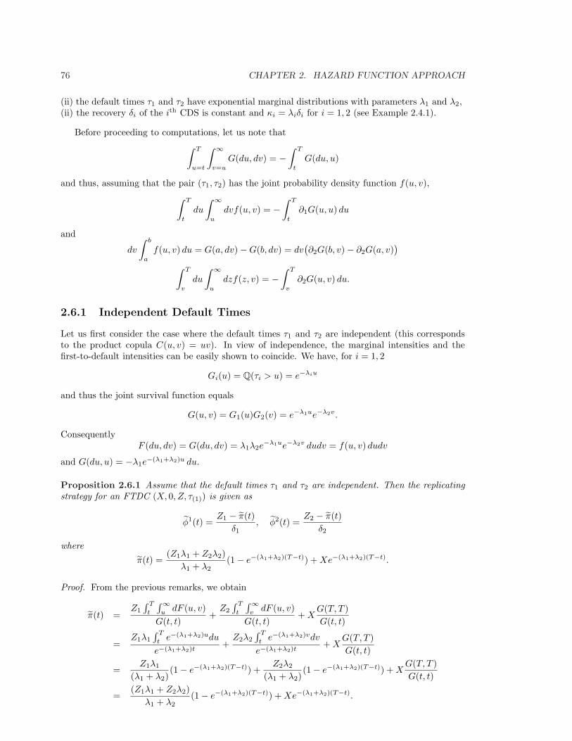
76 CHAPTER 2. HAZARD FUNCTION APPROACH
(ii) the default times τ1 and τ2 have exponential marginal distributions with parameters λ1 and λ2,(ii) the recovery δi of the ith CDS is constant and κi = λiδi for i = 1, 2 (see Example 2.4.1).
Before proceeding to computations, let us note that∫ T
u=t
∫ ∞
v=u
G(du, dv) = −∫ T
t
G(du, u)
and thus, assuming that the pair (τ1, τ2) has the joint probability density function f(u, v),∫ T
t
du
∫ ∞
u
dvf(u, v) = −∫ T
t
∂1G(u, u) du
and
dv
∫ b
a
f(u, v) du = G(a, dv)−G(b, dv) = dv(∂2G(b, v)− ∂2G(a, v)
)
∫ T
v
du
∫ ∞
u
dzf(z, v) = −∫ T
v
∂2G(u, v) du.
2.6.1 Independent Default Times
Let us first consider the case where the default times τ1 and τ2 are independent (this correspondsto the product copula C(u, v) = uv). In view of independence, the marginal intensities and thefirst-to-default intensities can be easily shown to coincide. We have, for i = 1, 2
Gi(u) = Q(τi > u) = e−λiu
and thus the joint survival function equals
G(u, v) = G1(u)G2(v) = e−λ1ue−λ2v.
ConsequentlyF (du, dv) = G(du, dv) = λ1λ2e
−λ1ue−λ2v dudv = f(u, v) dudv
and G(du, u) = −λ1e−(λ1+λ2)u du.
Proposition 2.6.1 Assume that the default times τ1 and τ2 are independent. Then the replicatingstrategy for an FTDC (X, 0, Z, τ(1)) is given as
φ1(t) =Z1 − π(t)
δ1, φ2(t) =
Z2 − π(t)δ2
where
π(t) =(Z1λ1 + Z2λ2)
λ1 + λ2(1− e−(λ1+λ2)(T−t)) + Xe−(λ1+λ2)(T−t).
Proof. From the previous remarks, we obtain
π(t) =Z1
∫ T
t
∫∞u
dF (u, v)G(t, t)
+Z2
∫ T
t
∫∞v
dF (u, v)G(t, t)
+ XG(T, T )G(t, t)
=Z1λ1
∫ T
te−(λ1+λ2)udu
e−(λ1+λ2)t+
Z2λ2
∫ T
te−(λ1+λ2)vdv
e−(λ1+λ2)t+ X
G(T, T )G(t, t)
=Z1λ1
(λ1 + λ2)(1− e−(λ1+λ2)(T−t)) +
Z2λ2
(λ1 + λ2)(1− e−(λ1+λ2)(T−t)) + X
G(T, T )G(t, t)
=(Z1λ1 + Z2λ2)
λ1 + λ2(1− e−(λ1+λ2)(T−t)) + Xe−(λ1+λ2)(T−t).

2.6. APPLICATIONS TO COPULA-BASED CREDIT RISK MODELS 77
Under the assumption of independence of default times, we also have that Sit|j(κi) = Si
t(κi) for
i, j = 1, 2 and i 6= j. Furthermore from Example 2.4.1, we have that Sit(κi) = 0 for t ∈ [0, T ] and
thus the matrix N(t) in Theorem 2.2 reduces to
N(t) =[
δ1 00 δ2
].
The replicating strategy can be found easily by solving the linear equation N(t)φ(t) = h(t) whereh(t) = (h1(t), h2(t)) with hi(t) = Zi − π(t−) = Zi − π(t) for i = 1, 2. ¤
As another important case of a first-to-default claim, we take a first-to-default swap (FTDS). Fora stylized FTDS we have X = 0, A(t) = −κ(1)t where κ(1) is the swap spread, and Zi(t) = δi ∈ [0, 1)for some constants δi, i = 1, 2. Hence an FTDS is formally given as an FTDC (0,−κ(1)t, (δ1, δ2), τ(1)).
Under the present assumptions, we easily obtain
π0 = π(0) =1− eλT
λ
((λ1δ1 + λ2δ2)− κ(1)
)
where λ = λ1 + λ2. The FTDS market spread is the level of κ(1) that makes the FTDS valueless atinitiation. Hence in this elementary example this spread equals λ1δ1 + λ2δ2. In addition, it can beshown that under the present assumptions we have that π(t) = 0 for every t ∈ [0, T ].
Suppose that we wish to hedge the short position in the FTDS using two CDSs, say CDSi,i = 1, 2, with respective default times τi, protection payments δi and spreads κi = λiδi. Recall thatin the present setup we have that, for t ∈ [0, T ],
Sit|j(κi) = Si
t(κi) = 0, i, j = 1, 2, i 6= j. (2.102)
Consequently, we have here that hi(t) = −Zi(t) = −δi for every t ∈ [0, T ]. It then follows fromequation N(t)φ(t) = h(t) that φ1(t) = φ2(t) = 1 for every t ∈ [0, T ] and thus φ0
t = 0 for everyt ∈ [0, T ]. This result is by no means surprising: we hedge a short position in the FTDS byholding a static portfolio of two single-name CDSs since, under the present assumptions, the FTDSis equivalent to such a portfolio of corresponding single name CDSs. Of course, one would not expectthat this feature will still hold in a general case of dependent default times.
The first equality in (2.102) is due to the standing assumption of independence of default timesτ1 and τ2 and thus it will no longer be true for other copulas (see foregoing subsections). The secondequality follows from the postulate that the risk-neutral marginal distributions of default times areexponential. In practice, the risk-neutral marginal distributions of default times will be obtained byfitting the model to market data (i.e., market prices of single name CDSs) and thus typically theywill not be exponential. To conclude, both equalities in (2.102) are unlikely to hold in any real-lifeimplementation. Hence this example show be seen as the simplest illustration of general results andwe do not pretend that it has any practical merits.
2.6.2 Archimedean Copulas
We now proceed to the case of exponentially distributed, but dependent, default times. Theirinterdependence will be specified by a choice of some Archimedean copula. Recall that a bivariateArchimedean copula is defined as C(u, v) = ϕ−1(ϕ(u), ϕ(v)), where ϕ is called the generator of acopula.
Clayton Copula
Recall that the generator of the Clayton copula is given as ϕ(s) = s−θ − 1, s ∈ R+, for some strictlypositive parameter θ. Hence the bivariate Clayton copula can be represented as follows
C(u, v) = CClaytonθ (u, v) = (u−θ + v−θ − 1)−
1θ .

78 CHAPTER 2. HAZARD FUNCTION APPROACH
Under the present assumptions, the corresponding joint survival function G(u, v) equals
G(u, v) = C(G1(u), G2(v)) = (eλ1uθ + eλ2vθ − 1)−1θ
so thatG(u, dv)
dv= −λ2e
λ2vθ(eλ1uθ + eλ2vθ − 1)−1θ−1
and
f(u, v) =G(du, dv)
dudv= (θ + 1)λ1λ2e
λ1uθ+λ2vθ(eλ1uθ + eλ2vθ − 1)−1θ−2.
Proposition 2.6.2 Let the joint distribution of (τ1, τ2) be given by the Clayton copula with θ > 0.Then the replicating strategy for an FTDC (X, 0, Z, τ(1)) is given by the expressions
φ1(t) =δ2(Z1 − π(t)) + S2
t|1(κ2)(Z2 − π(t))
δ1δ2 − S1t|2(κ1)S2
t|1(κ2), (2.103)
φ2(t) =δ1(Z2 − π(t)) + S1
t|2(κ1)(Z1 − π(t))
δ1δ2 − S1t|2(κ1)S2
t|1(κ2), (2.104)
where
π(t) = Z1
∫ eλ1θT
eλ1θt (s + sλ2λ1 − 1)−
1θ−1 ds
θ(eλ1θt + eλ2θt − 1)−1θ
+ Z2
∫ eλ2θT
eλ2θt (s + sλ1λ2 − 1)−
1θ−1 ds
θ(eλ1θt + eλ2θt − 1)−1θ
+ X(eλ1θT + eλ2θT − 1)−
1θ
(eλ1θt + eλ2θt − 1)−1θ
,
S1v|2(κ1) = δ1
[(eλ1θT + eλ2θT − 1)−1θ−1 − (eλ1θv + eλ2θv − 1)−
1θ−1]
(eλ1θv + eλ2θv − 1)−1θ−1
− κ1
∫ T
v(eλ1θu + eλ2θv − 1)−
1θ−1du
(eλ1θv + eλ2θv − 1)−1θ−1
,
and
S2u|1(κ2) = δ2
[(eλ1θT + eλ2θT − 1)−1θ−1 − (eλ1θu + eλ2θu − 1)−
1θ−1]
(eλ1θu + eλ2θu − 1)−1/θ−1
− κ2
∫ T
u(eλ1θu + eλ2θv − 1)−
1θ−1dv
(eλ1θu + eλ2θu − 1)−1θ−1
.
Proof. Using the observation that
∫ T
t
du
∫ ∞
u
f(u, v)dv =∫ T
t
λ1eλ1uθ(eλ1uθ + eλ2uθ − 1)−
1θ−1 du
=1θ
∫ eλ1θT
eλ1θt
(s + sλ2λ1 − 1)−
1θ−1 ds
and thus by symmetry
∫ T
t
dv
∫ ∞
v
f(u, v)du =1θ
∫ eλ2θT
eλ2θt
(s + sλ1λ2 − 1)−
1θ−1 ds.

2.6. APPLICATIONS TO COPULA-BASED CREDIT RISK MODELS 79
We thus obtain
π(t) =Z1
∫ T
t
∫∞u
dG(u, v)G(t, t)
+Z2
∫ T
t
∫∞v
dG(u, v)G(t, t)
+ XG(T, T )G(t, t)
= Z1
∫ eλ1θT
eλ1θt (s + sλ2λ1 − 1)−
1θ−1 ds
θ(eλ1θt + eλ2θt − 1)−1θ
+ Z2
∫ eλ2θT
eλ2θt (s + sλ1λ2 − 1)−
1θ−1 ds
θ(eλ1θt + eλ2θt − 1)−1θ
+ X(eλ1θT + eλ2θT − 1)−
1θ
(eλ1θt + eλ2θt − 1)−1θ
.
We are in a position to determine the replicating strategy. Under the standing assumption thatκi = λiδi for i = 1, 2 we still have that Si
t(κi) = 0 for i = 1, 2 and for t ∈ [0, T ]. Hence the matrixN(t) reduces to
N(t) =
[δ1 −S2
t|1(κ2)−S1
t|2(κ1) δ2
]
where
S1v|2(κ1) = δ1
∫ T
vf(u, v) du∫∞
vf(u, v) du
− κ1
∫ T
v
∫∞u
f(z, v) dzdu∫∞v
f(u, v) du
= δ1[(eλ1θT + eλ2θT − 1)−
1θ−1 − (eλ1θv + eλ2θv − 1)−
1θ−1]
(eλ1θv + eλ2θv − 1)−1θ−1
− κ1
∫ T
v(eλ1θu + eλ2θv − 1)−
1θ−1 du
(eλ1θv + eλ2θv − 1)−1θ−1
.
The expression for S2u|1(κ2) can be found by analogous computations. By solving the equation
N(t)φ(t) = h(t), we obtain the desired expressions (2.103)-(2.104). ¤
Similar computations can be done for the valuation and hedging of a first-to-default swap.
Gumbel Copula
As another of an Archimedean copula, we consider the Gumbel copula with the generator ϕ(s) =(− ln s)θ, s ∈ R+, for some θ ≥ 1. The bivariate Gumbel copula can thus be written as
C(u, v) = CGumbelθ (u, v) = e−[(− ln u)θ+(− ln v)θ]
1θ .
Under our standing assumptions, the corresponding joint survival function G(u, v) equals
G(u, v) = C(G1(u), G2(v)) = e−(λθ1uθ+λθ
2vθ)1θ .
ConsequentlydG(u, v)
dv= −G(u, v)λθ
2vθ−1(λθ
1uθ + λθ
2vθ)
1θ−1
anddG(u, v)
dudv= G(u, v)(λ1λ2)θ(uv)θ−1(λθ
1uθ + λθ
2vθ)
1θ−2
((λθ
1uθ + λθ
2vθ)
1θ + θ − 1
).
Proposition 2.6.3 Let the joint distribution of (τ1, τ2) be given by the Gumbel copula with θ ≥ 1.Then the replicating strategy for an FTDC (X, 0, Z, τ(1)) is given by (2.103)-(2.104) with
π(t) = (Z1λθ1 + Z2λ
θ2)λ
−θ(e−λt − e−λT ) + Xe−λ(T−t),

80 CHAPTER 2. HAZARD FUNCTION APPROACH
S1v|2(κ1) = δ1
e−(λθ1T θ+λθ
2vθ)1θ (λθ
1Tθ + λθ
2vθ)
1θ−1 − e−λvλ1−θv1−θ
e−λvλ1−θv1−θ
− κ1
∫ T
ve−(λθ
1T θ+λθ2vθ)
1θ (λθ
1uθ + λθ
2vθ)
1θ−1 du
e−λvλ1−θv1−θ,
S2u|1(κ2) = δ2
e−(λθ1uθ+λθ
2T θ)1θ (λθ
1uθ + λθ
2Tθ)
1θ−1 − e−λvλ1−θu1−θ
e−λvλ1−θu1−θ
− κ2
∫ T
ue−(λθ
1uθ+λθ2T θ)
1θ (λθ
1uθ + λθ
2vθ)
1θ−1 dv
e−λvλ1−θu1−θ.
Proof. We have
∫ T
t
∫ ∞
u
dG(u, v) =∫ T
t
λθ1(λ
θ1 + λθ
2)1θ−1e−(λθ
1+λθ2)
1θ u du
= (−λθ1λ−θe−λu)|u=T
u=t = λθ1λ−θ(e−λt − e−λT )
where λ = (λθ1 + λθ
2)1θ . Similarly
∫ T
t
∫ ∞
v
dG(u, v) = λθ2λ−θ(e−λt − e−λT ).
Furthermore G(T, T ) = e−λT and G(t, t) = e−λt. Hence
π(t) = Z1
∫ T
t
∫∞u
dG(u, v)G(t, t)
+ Z2
∫ T
t
∫∞v
dG(u, v)G(t, t)
+ XG(T, T )G(t, t)
= Z1λθ1λ−θ(e−λt − e−λT ) + Z2λ
θ2λ−θ(e−λt − e−λT ) + Xe−λ(T−t)
= (Z1λθ1 + δ2Z
θ2 )λ−θ(e−λt − e−λT ) + Xe−λ(T−t).
In order to find the replicating strategy, we proceed as in the proof of Proposition 2.6.2. Under thepresent assumptions, we have
S1v|2(κ1) = δ1
∫ T
vf(u, v)du∫∞
vf(u, v)du
− κ1
∫ T
v
∫∞u
f(z, v)dzdu∫∞v
f(u, v)du
= δ1e−(λθ
1T θ+λθ2vθ)
1θ (λθ
1Tθ + λθ
2vθ)
1θ−1 − e−λvλ1−θv1−θ
e−λvλ1−θv1−θ
− κ1
∫ T
ve−(λθ
1T θ+λθ2vθ)
1θ (λθ
1uθ + λθ
2vθ)
1θ−1du
e−λvλ1−θv1−θ.
This completes the proof. ¤

Chapter 3
Hazard Process Approach
In the general reduced-form (or hazard process) approach, we deal with two kinds of information: theinformation conveyed by the assets prices, denoted as F = (Ft)0≤t≤T∗ , and the information aboutthe occurrence of the default time, that is, the knowledge of the time where the default occurred inthe past, if the default has indeed already happen. As we already know, the latter information ismodeled by the filtration H generated by the default process H.
At the intuitive level, the reference filtration F is generated by prices of some assets, or by othereconomic factors (such as, e.g., interest rates). This filtration can also be a subfiltration of thefiltration generated by the asset prices. The case where F is the trivial filtration is exactly what wehave studied in the previous chapter. Though in a typical example F is chosen to be the Brownianfiltration, most theoretical results do not rely on a particular choice of the reference filtration F. Wedenote by Gt = Ft ∨Ht the full filtration (sometimes referred to as the enlarged filtration).
Special attention will be paid in this chapter to the so-called hypothesis (H), which, in the presentcontext, postulates the invariance of the martingale property with respect to the enlargement of F bythe observations of the default time. In order to examine the exact meaning of market completenessin a defaultable world and to derive the hedging strategies for credit derivatives, we shall alsoestablish a suitable version of the predictable representation theorem.
Most results presented in Sections 3.1-3.6 can be found, for instance, in survey papers by Bieleckiat al. [8] and Jeanblanc and Rutkowski [58, 59]. Sections 3.7-3.8 are based on Bielecki at al. [11].
3.1 Hazard Process and its Applications
The concepts introduced in the previous chapter will now be extended to a more general set-up, whenallowance for an additional flow of information – formally represented hereafter by some referencefiltration F – is made.
We denote by τ a non-negative random variable on a probability space (Ω,G,Q), satisfyingQ(τ = 0) = 0 and Q(τ > t) > 0 for any t ∈ R+. We introduce the right-continuous process H bysetting Ht = 1τ≤t and we denote by H the associated filtration, so that Ht = σ(Hu : u ≤ t) forevery t ∈ R+.
We assume that we are given an auxiliary reference filtration F such that G = H ∨ F, that is,Gt = Ht ∨ Ft for any t ∈ R+. For each t ∈ R+, the total information available at time t is capturedby the σ-field Gt.
All filtrations considered in what follows are implicitly assumed to satisfy the ‘usual conditions’of right-continuity and completeness. For the sake of simplicity, we assume that the σ-field F0 istrivial (so that G0 is a trivial σ-field as well).
81
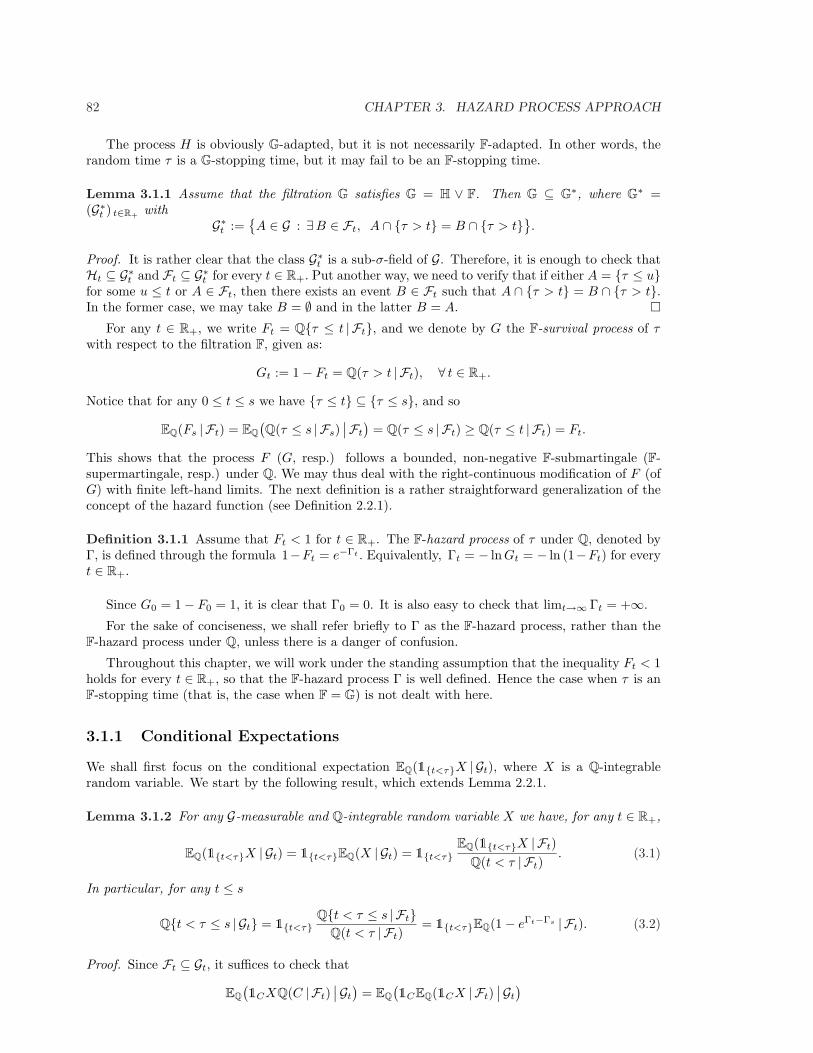
82 CHAPTER 3. HAZARD PROCESS APPROACH
The process H is obviously G-adapted, but it is not necessarily F-adapted. In other words, therandom time τ is a G-stopping time, but it may fail to be an F-stopping time.
Lemma 3.1.1 Assume that the filtration G satisfies G = H ∨ F. Then G ⊆ G∗, where G∗ =(G∗t ) t∈R+ with
G∗t :=A ∈ G : ∃B ∈ Ft, A ∩ τ > t = B ∩ τ > t.
Proof. It is rather clear that the class G∗t is a sub-σ-field of G. Therefore, it is enough to check thatHt ⊆ G∗t and Ft ⊆ G∗t for every t ∈ R+. Put another way, we need to verify that if either A = τ ≤ ufor some u ≤ t or A ∈ Ft, then there exists an event B ∈ Ft such that A ∩ τ > t = B ∩ τ > t.In the former case, we may take B = ∅ and in the latter B = A. ¤
For any t ∈ R+, we write Ft = Qτ ≤ t | Ft, and we denote by G the F-survival process of τwith respect to the filtration F, given as:
Gt := 1− Ft = Q(τ > t | Ft), ∀ t ∈ R+.
Notice that for any 0 ≤ t ≤ s we have τ ≤ t ⊆ τ ≤ s, and so
EQ(Fs | Ft) = EQ(Q(τ ≤ s | Fs)
∣∣Ft
)= Q(τ ≤ s | Ft) ≥ Q(τ ≤ t | Ft) = Ft.
This shows that the process F (G, resp.) follows a bounded, non-negative F-submartingale (F-supermartingale, resp.) under Q. We may thus deal with the right-continuous modification of F (ofG) with finite left-hand limits. The next definition is a rather straightforward generalization of theconcept of the hazard function (see Definition 2.2.1).
Definition 3.1.1 Assume that Ft < 1 for t ∈ R+. The F-hazard process of τ under Q, denoted byΓ, is defined through the formula 1−Ft = e−Γt . Equivalently, Γt = − ln Gt = − ln (1−Ft) for everyt ∈ R+.
Since G0 = 1− F0 = 1, it is clear that Γ0 = 0. It is also easy to check that limt→∞ Γt = +∞.
For the sake of conciseness, we shall refer briefly to Γ as the F-hazard process, rather than theF-hazard process under Q, unless there is a danger of confusion.
Throughout this chapter, we will work under the standing assumption that the inequality Ft < 1holds for every t ∈ R+, so that the F-hazard process Γ is well defined. Hence the case when τ is anF-stopping time (that is, the case when F = G) is not dealt with here.
3.1.1 Conditional Expectations
We shall first focus on the conditional expectation EQ(1t<τX | Gt), where X is a Q-integrablerandom variable. We start by the following result, which extends Lemma 2.2.1.
Lemma 3.1.2 For any G-measurable and Q-integrable random variable X we have, for any t ∈ R+,
EQ(1t<τX | Gt) = 1t<τEQ(X | Gt) = 1t<τEQ(1t<τX | Ft)Q(t < τ | Ft)
. (3.1)
In particular, for any t ≤ s
Qt < τ ≤ s | Gt = 1t<τQt < τ ≤ s | FtQ(t < τ | Ft)
= 1t<τEQ(1− eΓt−Γs | Ft). (3.2)
Proof. Since Ft ⊆ Gt, it suffices to check that
EQ(1CXQ(C | Ft)
∣∣Gt
)= EQ
(1CEQ(1CX | Ft)
∣∣Gt
)

3.1. HAZARD PROCESS AND ITS APPLICATIONS 83
where we denote C = t < τ. Put another way, we need to show that for any A ∈ Gt we have∫
A
1CXQ(C | Ft) dQ =∫
A
1CEQ(1CX | Ft) dQ.
In view of Lemma 3.1.1, for any A ∈ Gt we have A ∩ C = B ∩ C for some event B ∈ Ft. Therefore,∫
A
1CXQ(C | Ft) dQ =∫
A∩C
XQ(C | Ft) dQ =∫
B∩C
XQ(C | Ft) dQ
=∫
B
1CXQ(C | Ft) dQ =∫
B
EQ(1CX | Ft)Q(C | Ft) dQ
=∫
B
EQ(1CEQ(1CX | Ft) | Ft) dQ =∫
B∩C
EQ(1CX | Ft) dQ
=∫
A∩C
EQ(1CX | Ft) dQ =∫
A
1CEQ(1CX | Ft) dQ
as desired. ¤The following corollary to Lemma 3.1.2 is rather straightforward (note that to obtain the second
equality in (3.3), it suffices to condition on the σ-field Fs).
Corollary 3.1.1 Let X be an Fs-measurable and Q-integrable random variable. Then, for everyt ≤ s,
EQ(X1s<τ | Gt) = 1t<τEQ(X1s<τ | Ft)EQ(1t<τ | Ft)
= 1t<τEQ(XeΓt−Γs | Ft). (3.3)
The proof of the next result, based on an approximation of the process Z by a suitable sequenceof step-wise processes, is left to the reader.
Proposition 3.1.1 Assume that Z is an F-predictable process such that the random variable Zτ1τ≤sis Q-integrable. Then, for every t ≤ s,
1t<τEQ(Zτ1τ≤s | Gt) = 1t<τeΓt EQ(∫
]t,s]
Zu dFu
∣∣∣Ft
). (3.4)
Let F = N + C be the Doob-Meyer decomposition of F , where N is an F-martingale, with N0 = 0,and C is an F-predictable increasing process, with C0 = 0. Then, for every t ≤ s,
1t<τEQ(Zτ1τ≤s | Gt) = 1t<τeΓt EQ( ∫
]t,s]
Zu dCu
∣∣∣Ft
).
In particular, if F is an increasing, continuous process then F = C = 1−e−Γt so that dFt = e−Γt dΓt.Consequently,
1t<τEQ(Zτ1τ≤s | Gt) = 1t<τ EQ( ∫ s
t
ZueΓt−Γu dΓu
∣∣∣Ft
). (3.5)
The next result appears to be useful in valuation of defaultable securities that pay dividendsprior to the default time. The proof is also left to the reader as an exercise.
Proposition 3.1.2 Assume that A is a bounded, F-predictable process of finite variation. Then, forevery t ≤ s,
EQ( ∫
]t,s]
(1−Hu) dAu
∣∣∣Gt
)= 1t<τeΓtEQ
( ∫
]t,s]
(1− Fu) dAu
∣∣∣Ft
)
or, equivalently,
EQ( ∫
]t,s]
(1−Hu) dAu
∣∣∣Gt
)= 1t<τEQ
( ∫
]t,s]
eΓt−Γu dAu
∣∣∣Ft
).

84 CHAPTER 3. HAZARD PROCESS APPROACH
3.1.2 Stochastic Intensity
Assume that the process F is absolutely continuous, that is, Ft =∫ t
0fu du for some F-progressively
measurable, non-negative process f . Then necessarily F is an increasing process and thus Γ is anabsolutely continuous and increasing process as well. Specifically, it is easy to check that Γ admitsthe stochastic intensity (or hazard rate) γ, that is,
Γt =∫ t
0
γu du
where in turn the F-progressively measurable, non-negative process γ is given by the formula
γt =ft
1− Ft.
3.1.3 Valuation of Defaultable Claims
Our next goal is to establish a convenient representation for the pre-default value of a defaultableclaim in terms of the hazard process Γ of the default time. We postulate that Q represents amartingale measure associated with the choice of the savings account B as a discount factor (ornumeraire). Hence, in the present set-up, the risk-neutral valuation formula reads
St = Bt EQ( ∫
]t,T ]
B−1u dDu
∣∣∣Gt
). (3.6)
where S is the ex-dividend price process and D is the dividend process associated with a defaultableclaim (see Section 1.1.2), that is,
Dt = Xd(T )1t≥T +∫
]0,t]
(1−Hu) dAu +∫
]0,t]
Zu dHu. (3.7)
Finally, B stands for the savings account process, that is,
Bt = exp(∫ t
0
ru du)
where the F-progressively measurable process r models the short-term interest rate.
For the sake of conciseness, we will write
It = Bt EQ( ∫
]t,T ]
B−1u (1−Hu) dAu
∣∣∣Gt
),
Jt = Bt EQ(1t<τ≤TB−1
τ Zτ
∣∣Gt
),
andKt = Bt EQ
(B−1
T X1T<τ∣∣Gt
).
In view of (3.6)–(3.7), it is clear that the ex-dividend price of a defaultable claim (X,A, 0, Z, τ)satisfies St = It + Jt + Kt.
Proposition 3.1.3 The ex-dividend price of a defaultable claim (X, A, 0, Z, τ) admits the followingrepresentation, for every t ∈ [0, T ],
St = 1t<τG−1t Bt EQ
( ∫
]t,T ]
B−1u (Gu dAu − Zu dGu) + GT B−1
T X∣∣∣Ft
).
If F (and thus also Γ) is an increasing, continuous process then
St = 1t<τBt EQ( ∫
]t,T ]
B−1u eΓt−Γu (dAu + Zu dΓu) + B−1
T XeΓt−ΓT
∣∣∣Ft
).

3.1. HAZARD PROCESS AND ITS APPLICATIONS 85
Proof. By applying Proposition 3.1.2 to the process of finite variation∫]0,t]
B−1u dAu, we obtain
It = 1t<τG−1t Bt EQ
(∫
]t,T ]
B−1u Gu dAu
∣∣∣Ft
)
or, equivalently,
It = 1t<τBt EQ(∫
]t,T ]
B−1u eΓt−Γu dAu
∣∣∣Ft
).
Furthermore, formula (3.4) of Proposition 3.1.1 yields
Jt = 1t<τeΓtBt EQ( ∫
]t,T ]
B−1u Zu dFu
∣∣∣Ft
).
If, in addition, the hazard process Γ is an increasing continuous process then
Jt = 1t<τBt EQ(∫ T
t
B−1u eΓt−ΓuZu dΓu
∣∣∣Ft
).
Finally, it follows from (3.1) that
Kt = 1t<τeΓtBt EQ(1τ>TB−1T X | Ft).
Since the random variables X and BT are FT -measurable, we also have (see (3.3))
Kt = 1t<τeΓtBt EQ(GT B−1T X | Ft) = 1t<τBt EQ
(B−1
T XeΓt−ΓT | Ft
).
Both formulae of the proposition are obtained upon summation. ¤Let us note that St = 1t<τSt, where the F-adapted process S represents the pre-default value
of the claim (X, A, 0, Z, τ). The following result is an immediate consequence of Proposition 3.1.3.
Corollary 3.1.2 Assume that F (and thus also Γ) is an increasing, continuous process. Thenthe pre-default value of a defaultable claim (X, A, 0, Z, τ) coincides with the pre-default value of adefaultable claim (X, A, 0, 0, τ), where At = At +
∫ t
0Zu dΓu.
Remark 3.1.1 We have omitted in Proposition 3.1.3 the recovery payoff X, since the expressionbased on the hazard process of the default time does not easily cover the case of a general FT -measurable random variable. However, in the special case when X = δ for some constant δ, itsuffices to substitute X with an equivalent payoff δB(τ, T ) at time of default.
Let us return to the case of the default time that admits the stochastic intensity γ. The secondformula of Proposition 3.1.3 now takes the following form
St = 1t<τ EQ( ∫
]t,T ]
e−∫ u
t(rv+γv)dv (dAu + γuZu du)
∣∣∣Ft
)
+ 1t<τ EQ(e−
∫ Tt
(rv+γv)dvX∣∣∣Ft
).
To get a more concise representation for the last expression, we introduce the default-risk-adjustedinterest rate r = r + γ and the associated default-risk-adjusted savings account B, given by theformula
Bt = exp( ∫ t
0
ru du). (3.8)
Although the process B does not represent the price of a tradeable security, it has similar featuresas the savings account B. In particular, B is an F-adapted, continuous process of finite variation.In terms of the process B, we have
St = 1t<τBt EQ( ∫
]t,T ]
B−1u dAu +
∫ T
t
B−1u Zuγu du + B−1
T X∣∣∣Ft
). (3.9)
It is noteworthy that the default time τ does not appear explicitly in the conditional expectation onthe right-hand side of (3.9).

86 CHAPTER 3. HAZARD PROCESS APPROACH
3.1.4 Martingales Associated with Default Time
We will now examine some important martingales associated with the default time τ .
Proposition 3.1.4 (i) The process Lt = (1−Ht)eΓt is a G-martingale.(ii) If X is an F-martingale and the process XL is integrable then it is a G-martingale.(iii) If the process F (or, equivalently, Γ) is increasing and continuous then the process Mt =Ht − Γ(t ∧ τ) is a G-martingale.
Proof. (i) From Lemma 3.1.2, we obtain, for any t ≤ s,
EQ(Ls | Gt) = 1t<τeΓtEQ(1s<τeΓs | Ft) = 1t<τeΓt = Lt,
since the tower rule yields
EQ(1s<τeΓs |Ft) = EQ(EQ(1s<τ | Fs)eΓs |Ft) = 1.
(ii) Using again Lemma 3.1.2, we get, for any t ≤ s,
EQ(LsXs | Gt) = EQ(1s<τLsXs | Gt)
= 1t<τeΓt EQ(1s<τe−ΓsXs
∣∣Ft
)
= 1t<τeΓt EQ(EQ(1s<τ | Fs)e−ΓsXs
∣∣Ft
)
= LtXt.
(iii) Note that H is a process of finite variation and Γ an increasing continuous process. Hence fromthe integration by parts formula, we obtain
dLt = (1−Ht)eΓt dΓt − eΓt dHt.
Moreover, the process Mt = Ht − Γ(t ∧ τ) can be represented as follows
Mt =∫
]0,t]
dHu −∫
]0,t]
(1−Hu) dΓu = −∫
]0,t]
e−Γu dLu,
and thus it is a G-martingale, since L is G-martingale and e−Γt is a bounded process. It should bestressed that if the hazard process Γ is not increasing then the computation of the Ito differentialdeΓt is more complicated and part (iii) of the proposition is no longer true, in general. ¤
Note that the process F (or, equivalently, Γ) is not necessarily of finite variation. Hence part(iii) in Proposition 3.1.4 does not yield the general form of the Doob-Meyer decomposition of thesubmartingale H. For simplicity, in the next result we shall assume that F is a continuous process.It is worth noting that part (iii) in Proposition 3.1.4 is also a consequence of Proposition 3.1.5, sincefor a continuous and increasing process F we have that F = C = 1− e−Γt .
Proposition 3.1.5 Assume that F is a continuous process with the Doob-Meyer decompositionF = N + C. Then the process M = (Mt, t ∈ R+), given by the formula
Mt = Ht −∫ t∧τ
0
dCu
1− Fu, (3.10)
is a G-martingale.
Proof. We split the proof into two steps.
First step. We shall prove that, for any t ≤ s,
EQ(Hs | Gt) = Ht + 1t<τeΓt EQ(Cs − Ct | Ft). (3.11)
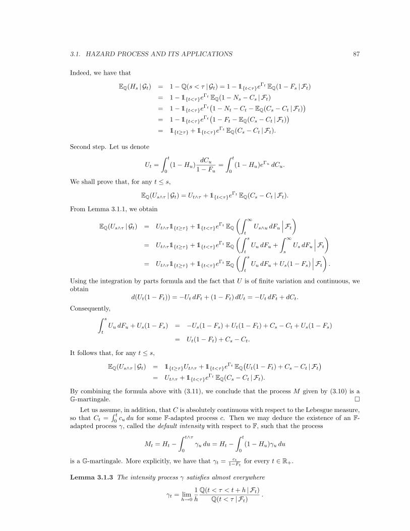
3.1. HAZARD PROCESS AND ITS APPLICATIONS 87
Indeed, we have that
EQ(Hs | Gt) = 1−Q(s < τ | Gt) = 1− 1t<τeΓt EQ(1− Fs | Ft)
= 1− 1t<τeΓt EQ(1−Ns − Cs | Ft)
= 1− 1t<τeΓt(1−Nt − Ct − EQ(Cs − Ct | Ft)
)
= 1− 1t<τeΓt(1− Ft − EQ(Cs − Ct | Ft)
)
= 1t≥τ + 1t<τeΓt EQ(Cs − Ct | Ft).
Second step. Let us denote
Ut =∫ t
0
(1−Hu)dCu
1− Fu=
∫ t
0
(1−Hu)eΓu dCu.
We shall prove that, for any t ≤ s,
EQ(Us∧τ | Gt) = Ut∧τ + 1t<τeΓt EQ(Cs − Ct | Ft).
From Lemma 3.1.1, we obtain
EQ(Us∧τ | Gt) = Ut∧τ1t≥τ + 1t<τeΓt EQ(∫ ∞
t
Us∧u dFu
∣∣∣Ft
)
= Ut∧τ1t≥τ + 1t<τeΓt EQ(∫ s
t
Uu dFu +∫ ∞
s
Us dFu
∣∣∣Ft
)
= Ut∧τ1t≥τ + 1t<τeΓt EQ(∫ s
t
Uu dFu + Us(1− Fs)∣∣∣Ft
).
Using the integration by parts formula and the fact that U is of finite variation and continuous, weobtain
d(Ut(1− Ft)) = −Ut dFt + (1− Ft) dUt = −Ut dFt + dCt.
Consequently,∫ s
t
Uu dFu + Us(1− Fs) = −Us(1− Fs) + Ut(1− Ft) + Cs − Ct + Us(1− Fs)
= Ut(1− Ft) + Cs − Ct.
It follows that, for any t ≤ s,
EQ(Us∧τ | Gt) = 1t≥τUt∧τ + 1t<τeΓt EQ(Ut(1− Ft) + Cs − Ct | Ft
)
= Ut∧τ + 1t<τeΓt EQ(Cs − Ct | Ft).
By combining the formula above with (3.11), we conclude that the process M given by (3.10) is aG-martingale. ¤
Let us assume, in addition, that C is absolutely continuous with respect to the Lebesgue measure,so that Ct =
∫ t
0cu du for some F-adapted process c. Then we may deduce the existence of an F-
adapted process γ, called the default intensity with respect to F, such that the process
Mt = Ht −∫ t∧τ
0
γu du = Ht −∫ t
0
(1−Hu)γu du
is a G-martingale. More explicitly, we have that γt = ct
1−Ftfor every t ∈ R+.
Lemma 3.1.3 The intensity process γ satisfies almost everywhere
γt = limh→0
1h
Q(t < τ < t + h | Ft)Q(t < τ | Ft)
.

88 CHAPTER 3. HAZARD PROCESS APPROACH
Proof. The martingale property of M implies that
EQ(1t<τ<t+h | Gt)−∫ t+h
t
EQ((1−Hu)γu | Gt) du = 0.
By projecting on the σ-field Ft, we obtain
Q(t < τ < t + h | Ft) =∫ t+h
t
γuQ(u < τ | Ft) du.
The assertion of the lemma now easily follows. ¤
3.1.5 Reduction of the Reference Filtration
In this section, we follow Jeanblanc and LeCam [57]. Suppose that F is a sub-filtration of F, so thatFt ⊂ Ft for every t ∈ R+. We define the full filtration G by setting Gt = Ft ∨ Ht for every t ∈ R+.The hazard process of τ with respect to F is given by Γt = − ln(Gt) with
Gt = Q(t < τ | Ft) = EQ(Gt | Ft).
For any Q-integrable random variable Y , Lemma 3.1.2 implies that
EQ(1t<τY | Gt) = 1t<τeΓt EQ(1t<τY | Ft).
In particular, if Y is a FT -measurable random variable then
EQ(1T<τY | Gt) = 1t<τeΓt EQ(GT Y | Ft).
From the obvious equality
EQ(1T<τY | Gt) = EQ(EQ(1T<τY | Gt) | Gt),
we also obtain
EQ(1T<τY | Gt) = EQ(1t<τeΓt EQ(GT Y | Ft) | Gt
)
= 1t<τeΓt EQ(1t<τeΓt EQ(GT Y | Ft)
∣∣ Ft
).
From the uniqueness of the pre-default F-adapted process, it can now be deduced that the followingresult is true.
Lemma 3.1.4 For any Q-integrable and FT -measurable random variable Y we have, for any t ∈ R+,
EQ(GT Y | Ft) = EQ(1t<τeΓt EQ(GT Y | Ft)
∣∣ Ft
). (3.12)
Proof. We provide a direct proof of (3.12). We have
EQ(1t<τEQ(GT Y | Ft)eΓt
∣∣ Ft
)= EQ
(EQ(1t<τ | Ft)eΓt EQ(GT Y | Ft)
∣∣ Ft
)
= EQ(EQ(GT Y | Ft)
∣∣∣ Ft
)= EQ(GT Y | Ft)
= EQ(EQ(GT | FT )Y
∣∣∣ Ft
)= EQ(GT Y | Ft),
since we assumed that Y is FT -measurable. ¤

3.1. HAZARD PROCESS AND ITS APPLICATIONS 89
Let F = N + C be the Doob-Meyer decomposition of the submartingale F with respect to Fand let us assume that C is differentiable with respect to t, that is, Ct =
∫ t
0cu du. Since C is an
increasing process, it is easily seen that the process Ct = EQ(Ct | Ft) is a submartingale with respectto F. Let us denote by C = z + α its Doob-Meyer decomposition with respect to F and let us setNt = EQ(Nt | Ft). Since N is an F-martingale, we see that the submartingale
Ft = Q(t ≥ τ | Ft) = EQ(Ft | Ft)
admits the Doob-Meyer decomposition F = m + α, where the F-martingale part equals m = N + z.The next lemma furnishes an explicit link between the increasing processes C and α.
Lemma 3.1.5 Let Ct =∫ t
0cu du be the F-predictable increasing process in the Doob-Meyer decom-
position of the F-submartingale F . Then the F-predictable increasing process in the Doob-Meyerdecomposition of the F-submartingale F equals, for any t ∈ R+,
αt =∫ t
0
EQ(cu | Fu) du.
Proof. It suffices to prove that the process
MFt = EQ(Ft | Ft)−
∫ t
0
EQ(cu | Fu) du
is an F-martingale. Clearly, the process MF is integrable and F-adapted. Moreover,
EQ(MFT | Ft) = EQ
(EQ(FT | FT )−
∫ T
0
EQ(cu | Fu) du∣∣∣ Ft
)
= EQ(FT | Ft)− EQ( ∫ t
0
EQ(cu | Fu) du∣∣∣ Ft
)− EQ
(∫ T
t
EQ(cu | Fu) du∣∣∣ Ft
)
= Zt + EQ( ∫ t
0
cu du∣∣∣ Ft
)+ EQ
( ∫ T
t
cu du∣∣∣ Ft
)
−∫ t
0
EQ(cu | Fu) du− EQ( ∫ T
t
EQ(cu | Fu) du∣∣∣ Ft
)
= MFt + EQ
( ∫ T
t
cu du∣∣∣ Ft
)− EQ
(∫ T
t
EQ(cu | Fu) du∣∣∣ Ft
)
= MFt +
∫ T
t
EQ(cu | Ft) du−∫ T
t
EQ(EQ(cu | Fu)
∣∣∣ Ft
)du
= MFt +
∫ T
t
EQ(cu | Ft) du−∫ T
t
EQ(cu | Ft) du = MFt .
Hence the process MF is an F-martingale and the continuous process∫ .
0EQ(cu | Fu) du is clearly
F-predictable. The uniqueness of the Doob-Meyer decomposition implies that
αt =∫ t
0
EQ(cu | Fu) du,
as was claimed. ¤
Remark 3.1.2 Let us denote ct = EQ(ct | Ft). It follows that
Ht −∫ t∧τ
0
cu
1− Fu
du
is a G-martingale and that the F-intensity of τ is equal to EQ(ct | Ft)/Gt and not, as one mightexpect, to EQ(ct/Gt | Ft).

90 CHAPTER 3. HAZARD PROCESS APPROACH
3.1.6 Enlargement of Filtration
Assume that G is any enlarged filtration. Then we may work directly with the filtration G, providedthat the decomposition of any F-martingale in this filtration is known up to time τ . For example, if Wis an F-Brownian motion then it is not necessarily a G-martingale and its Doob-Meyer decompositionwith respect to the G filtration up to time τ reads
Wt∧τ = Ct∧τ +∫ t∧τ
0
d〈W,G〉uGu−
,
where (Ct∧τ , t ∈ R+) is a continuous G-martingale with the associated increasing process t ∧ τ .Suppose, for instance, that the dynamics of an asset S are given by
dSt = St
(rt dt + σt dWt
)
in a default-free framework (i.e., with respect to the filtration F). Then its dynamics with respectto the enlarged filtration G are
dSt = St
(rt dt + σt
d〈W,G〉tGt−
+ σt dCt
)
provided that we restrict our attention to the behavior of S prior to default. We conclude that thepossibility of default changes the drift term in the price dynamics. The interested reader is referredto Mansuy and Yor [74] for more information.
3.2 Hypothesis (H)
As mentioned above, an F-martingales does not remain a G-martingale, in general. We shall nowstudy a particular case in which this “martingale invariance property” holds.
3.2.1 Equivalent Formulations
Once again we consider a general situation where G = H ∨ F for some reference filtration F. Weshall now examine the hypothesis (H) which reads:
(H) Every F-local martingale is a G-local martingale.
This hypothesis implies, for instance, that any F-Brownian motion remains a Brownian motionwith respect to the enlarged filtration G. It was studied, among others by, Bremaud and Yor [21],Mazziotto and Szpirglas [75], and for financial purpose by Kusuoka [63]. Let us first examine someequivalent forms of hypothesis (H) (see, e.g., Dellacherie and Meyer [37]).
Lemma 3.2.1 Assume that G = F∨H, where F is an arbitrary filtration and H is generated by theprocess Ht = 1τ≤t. Then the following conditions are equivalent to the hypothesis (H) .(i) For any t, h ∈ R+, we have
Q(τ ≤ t | Ft) = Q(τ ≤ t | Ft+h). (3.13)
(i′) For any t ∈ R+, we haveQ(τ ≤ t | Ft) = Q(τ ≤ t | F∞). (3.14)
(ii) For any t ∈ R+, the σ-fields F∞ and Gt are conditionally independent given Ft under Q, thatis,
EQ(ξ η | Ft) = EQ(ξ | Ft)EQ(η | Ft)
for any bounded, F∞-measurable random variable ξ and bounded, Gt-measurable random variable η.(iii) For any t ∈ R+, and any u ≥ t the σ-fields Fu and Gt are conditionally independent given Ft.(iv) For any t ∈ R+ and any bounded, F∞-measurable random variable ξ: EQ(ξ | Gt) = EQ(ξ | Ft).(v) For any t ∈ R+, and any bounded, Gt-measurable random variable η: EQ(η | Ft) = EQ(η | F∞).

3.2. HYPOTHESIS (H) 91
Proof. If the hypothesis (H) holds then (3.14) is valid as well. If (3.14) holds then the fact thatHt is generated by the sets τ ≤ s, s ≤ t proves that F∞ and Ht are conditionally independentgiven Ft. The desired property now follows. This result can be also found in [38]. The equivalencebetween (3.14) and (3.13) is left to the reader.
Using the monotone class theorem, it can be shown that conditions (i) and (i′) are equivalent.The proof of equivalence of conditions (i′)–(v) can be found, for instance, in Section 6.1.1 of Bieleckiand Rutkowski [12] (for related results, see Elliott et al. [46]). Hence we shall only show thatcondition (iv) and the hypothesis (H) are equivalent.
Assume first that the hypothesis (H) holds. Consider any bounded, F∞-measurable randomvariable ξ. Let Mt = EQ(ξ | Ft) be the martingale associated with ξ. Of course, M is a localmartingale with respect to F. Then the hypothesis (H) implies that M is also a local martingalewith respect to G, and thus a G-martingale, since M is bounded (recall that any bounded localmartingale is a martingale). We conclude that Mt = EQ(ξ | Gt) and thus (iv) holds.
Suppose now that (iv) holds. First, we note that the standard truncation argument shows thatthe boundedness of ξ in (iv) can be replaced by the assumption that ξ is Q-integrable. Hence anyF-martingale M is an G-martingale, since M is clearly G-adapted and we have, for every t ≤ s,
Mt = EQ(Ms | Ft) = EQ(Ms | Gt),
where the second equality follows from (iv). Suppose now that M is an F-local martingale. Thenthere exists an increasing sequence of F-stopping times τn such that limn→∞ τn = ∞, for any n thestopped process Mτn follows a uniformly integrable F-martingale. Hence Mτn is also a uniformlyintegrable G-martingale, and this means that M is a G-local martingale. ¤
Remarks 3.2.1 (i) Equality (3.14) appears in numerous papers on default risk, typically withoutany reference to the hypothesis (H). For example, in Madan and Unal [73], the main theorem followsfrom the fact that (3.14) holds (see the proof of B9 in the appendix of [73]). This is also the casefor the model studied by Wong [85].(ii) If τ is F∞-measurable and (3.14) holds then τ is an F-stopping time. If τ is an F-stopping timethen equality (3.13) holds.(iii) Though the hypothesis (H) is not necessarily valid, in general, it is satisfied when τ is constructedthrough the so-called canonical approach (or for Cox processes). It also holds when τ is independentof F∞ (see Greenfield [52]).(iv) If the hypothesis (H) holds then from the condition(v) If hypothesis (H) holds then from the condition
Q(τ ≤ t | Ft) = Q(τ ≤ t | F∞), ∀ t ∈ R+,
we deduce easily that F is an increasing process.
Comments 3.2.1 See Elliott et al. [46] for more comments. The property that F is increasing isequivalent to the fact that any F-martingale stopped at time τ is a G martingale. Nikeghbali andYor [80] proved that this is equivalent to EQ(Mτ ) = M0 for any bounded F-martingale M . Thehypothesis (H) was also studied by Florens and Fougere [49], who coined the term noncausality.
Proposition 3.2.1 Assume that the hypothesis (H) holds. If X is an F-martingale then the pro-cesses XL and [L,X] are G-local martingales.
Proof. From Proposition 3.1.4(ii), the process XL is a G-martingale. Since
[L,X]t = LtXt −∫
]0,t]
Lu− dXu −∫
]0,t]
Xu− dLu,
and X is an F-martingale (and thus also a G-martingale), the process [L,X] is manifestly a G-localmartingale as the sum of three G-local martingales. ¤

92 CHAPTER 3. HAZARD PROCESS APPROACH
3.2.2 Canonical Construction of a Default Time
We shall now briefly describe the most commonly used construction of a default time associatedwith a given hazard process Γ. It should be stressed that the random time obtained through thisparticular method – which will be called the canonical construction in what follows – has certainspecific features that are not necessarily shared by all random times with a given F-hazard processΓ. We assume that we are given an F-adapted, right-continuous, increasing process Γ defined ona filtered probability space (Ω,G,Q). As usual, we assume that Γ0 = 0 and Γ∞ = +∞. In manyinstances, Γ is given by the equality
Γt =∫ t
0
γu du, ∀ t ∈ R+,
for some non-negative, F-progressively measurable intensity process γ.
To construct a random time τ , we shall postulate that the underlying probability space (Ω,G,Q)is sufficiently rich to support a random variable ξ, which is uniformly distributed on the interval[0, 1] and independent of the filtration F under Q. In this version of the canonical construction, Γrepresents the F-hazard process of τ under Q.
We define the random time τ : Ω → R+ by setting
τ = inf t ∈ R+ : e−Γt ≤ ξ = inf t ∈ R+ : Γt ≥ η , (3.15)
where the random variable η = − ln ξ has a unit exponential law under Q. It is not difficult to findthe process Ft = Q(τ ≤ t | Ft). Indeed, since clearly τ > t = ξ < e−Γt and the random variableΓt is F∞-measurable, we obtain
Q(τ > t | F∞) = Q(ξ < e−Γt | F∞) = Q(ξ < e−x)x=Γt = e−Γt . (3.16)
Consequently, we have
1− Ft = Q(τ > t | Ft) = EQ(Q(τ > t | F∞) | Ft
)= e−Γt , (3.17)
and so F is an F-adapted, right-continuous, increasing process. It is also clear that the process Γrepresents the F-hazard process of τ under Q. As an immediate consequence of (3.16) and (3.17),we obtain the following property of the canonical construction of the default time (cf. (3.14))
Q(τ ≤ t | F∞) = Q(τ ≤ t | Ft), ∀ t ∈ R+. (3.18)
To sum up, we have that
Q(τ ≤ t | F∞) = Q(τ ≤ t | Fu) = Q(τ ≤ t | Ft) = e−Γt (3.19)
for any two dates 0 ≤ t ≤ u.
3.2.3 Stochastic Barrier
Suppose thatQ(τ ≤ t | Ft) = Q(τ ≤ t | F∞) = 1− e−Γt ,
where Γ is a continuous, strictly increasing, F-adapted process. Our goal is to show that thereexists a random variable Θ, independent of F∞, with exponential law of parameter 1, such thatτ = inf t ≥ 0 : Γt > Θ. Let us set Θ := Γτ . Then
t < Θ = t < Γτ = Ct < τ,where C is the right inverse of Γ, so that ΓCt = t. Therefore
Q(Θ > u | F∞) = e−ΓCu = e−u.
We have thus established the required properties, namely, the probability law of Θ and its indepen-dence of the σ-field F∞. Furthermore, τ = inft : Γt > Γτ = inft : Γt > Θ.

3.3. PREDICTABLE REPRESENTATION THEOREM 93
3.3 Predictable Representation Theorem
Kusuoka [63] established the following representation theorem in which the reference filtration F isgenerated by a Brownian motion.
Theorem 3.1 Assume that the hypothesis (H) holds. Then any square-integrable martingale withrespect to G admits a representation as the sum of a stochastic integral with respect to the Brownianmotion and a stochastic integral with respect to the discontinuous martingale M associated with τ .
We assume, for simplicity, that F is continuous and Ft < 1 for every t ∈ R+. Since the hypothesis(H) holds, F is an increasing process. Then clearly
dFt = e−Γt dΓt, deΓt = eΓt dΓt. (3.20)
Proposition 3.3.1 Suppose that hypothesis (H) holds under Q and that any F-martingale is con-tinuous. Then the martingale Mh
t = EQ(hτ | Gt), where h is an F-predictable process such thatEQ|hτ | < ∞, admits the following decomposition in the sum of a continuous martingale and adiscontinuous martingale
Mht = mh
0 +∫ t∧τ
0
eΓu dmhu +
∫
]0,t∧τ ]
(hu −Mhu−) dMu, (3.21)
where mh is the continuous F-martingale given by
mht = EQ
( ∫ ∞
0
hu dFu
∣∣∣Ft
)
and M is the discontinuous G-martingale defined as Mt = Ht − Γt∧τ .
Proof. We start by noting that
Mht = EQ(hτ | Gt) = 1t≥τhτ + 1τ>teΓt EQ
( ∫ ∞
t
hu dFu
∣∣∣Ft
)
= 1t≥τhτ + 1τ>teΓt
(mh
t −∫ t
0
hu dFu
). (3.22)
We will sketch two slightly different derivations of (3.21).
First derivation. Let the process J be given by the formula, for t ∈ R+,
Jt = eΓt
(mh
t −∫ t
0
hu dFu
).
Noting that Γ is a continuous increasing process and mh is a continuous martingale, we deduce fromthe Ito integration by parts formula that
dJt = eΓt dmht − eΓtht dFt +
(mh
t −∫ t
0
hu dFu
)eΓt dΓt
= eΓt dmht − eΓtht dFt + Jt dΓt.
Therefore, from (3.20),dJt = eΓt dmh
t + (Jt − ht) dΓt
or, in the integrated form,
Jt = Mh0 +
∫ t
0
eΓu dmhu +
∫ t
0
(Ju − hu) dΓu.

94 CHAPTER 3. HAZARD PROCESS APPROACH
Note that Jt = Mht = Mh
t− on the event t < τ. Therefore, on the event t < τ,
Mht = Mh
0 +∫ t∧τ
0
eΓu dmhu +
∫ t∧τ
0
(Mhu− − hu) dΓu.
From (3.22), the jump of Mh at time τ is hτ − Jτ = hτ −Mhτ− = Mh
τ −Mhτ−. Equality (3.21) now
follows.
Second derivation. Equality (3.22) can be re-written as follows
Mht =
∫ t
0
hu dHu + (1−Ht)eΓt
(mh
t −∫ t
0
hu dFu
).
Hence the result can be obtained directly by the Ito integration by parts formula. ¤
3.4 Girsanov’s Theorem
We now start by defining a random time τ on a probability space (Ω,G,Q) and we postulate thatit admits the continuous F-hazard process Γ under Q. Hence, from Proposition 3.1.5, we know thatthe process Mt = Ht−Γt∧τ is a G-martingale. We postulate that the hypothesis (H) holds under Q.Finally, we postulate that the reference filtration F is generated by an F- (hence also G-) Brownianmotion under Q.
Let us fix T > 0. For a probability measure P equivalent to Q on (Ω,GT ) we introduce theG-martingale ηt, t ≤ T, by setting
ηt :=dPdQ
∣∣∣ Gt = EQ(X | Gt), Q-a.s., (3.23)
where X is a GT -measurable random variable, such that Q(X > 0) = 1 and EQX = 1.
Using Theorem 3.1, we deduce that the Radon-Nikodym density process η admits the followingrepresentation
ηt = 1 +∫ t
0
ξu dWu +∫
]0,t]
ζu dMu,
where ξ and ζ are G-predictable stochastic processes. Since η is a strictly positive process, we get
ηt = 1 +∫
]0,t]
ηu−(θu dWu + κu dMu
)(3.24)
where θ and κ are G-predictable processes, with κ > −1. More explicitly, the process η equals
ηt = Et
(∫ ·
0
θu dWu
)Et
(∫ ·
0
κu dMu
)= η
(1)t η
(2)t , (3.25)
where we write
η(1)t = Et
(∫ ·
0
θu dWu
)= exp
(∫ t
0
θu dWu − 12
∫ t
0
θ2u du
),
and
η(2)t = Et
(∫ ·
0
κu dMu
)= exp
(∫ t
0
ln(1 + κu) dHu −∫ t∧τ
0
κuγu du
). (3.26)
Then we have the following extension of Girsanov’s theorem.
Proposition 3.4.1 Let P be a probability measure on (Ω,GT ) equivalent to Q. If the Radon-Nikodymdensity of P with respect to Q is given by (3.23) with η satisfying (3.24) then the process
Wt = Wt −∫ t
0
θu du, ∀ t ∈ [0, T ], (3.27)

3.4. GIRSANOV’S THEOREM 95
is a Brownian motion with respect to G under P and the process
Mt := Mt −∫ t∧τ
0
κu dΓu = Ht −∫ t∧τ
0
(1 + κu) dΓu, ∀ t ∈ [0, T ], (3.28)
is a G-martingale under P orthogonal to W .
Proof. Note first that for t ≤ T we have
d(ηtWt) = Wt dηt + ηt− dWt + d[W , η]t= Wt dηt + ηt− dWt − ηt−θt dt + ηt−θt d[W,W ]t= Wt dηt + ηt− dWt.
This shows that W is a G-martingale under P. Since the quadratic variation of W under P equals[W , W ]t = t and W is continuous, by virtue of Levy’s theorem it is clear that W is a Brownianmotion under P. Similarly, for t ≤ T
d(ηtMt) = Mt dηt + ηt− dMt + d[M, η]t= Mt dηt + ηt− dMt − ηt−κt dΓt∧τ + ηt−κt dHt
= Mt dηt + ηt−(1 + κt) dMt.
We conclude that M is a G-martingale under P. To conclude it is enough to observe that W is acontinuous process and M follows a process of finite variation. ¤
The proof of the next result hinges on the predictable representation theorem.
Corollary 3.4.1 Let Y be a G-martingale under P. Then Y admits the following decomposition
Yt = Y0 +∫ t
0
ξ∗u dWu +∫
]0,t]
ζ∗u dMu, (3.29)
where ξ∗ and ζ∗ are G-predictable stochastic processes.
Proof. Consider the process Y given by the formula
Yt =∫
]0,t]
η−1u− d(ηuYu)−
∫
]0,t]
η−1u−Yu− dηu.
It is clear that Y is a G-local martingale under Q. Notice also that Ito’s formula yields
η−1u− d(ηuYu) = dYu + η−1
u−Yu− dηu + η−1u− d[Y, η]u,
and thusYt = Y0 + Yt −
∫
]0,t]
η−1u− d[Y, η]u. (3.30)
From the predictable representation theorem, we know that
Yt = Y0 +∫ t
0
ξu dWu +∫
]0,t]
ζu dMu (3.31)
for some G-predictable processes ξ and ζ. Therefore,
dYt = ξt dWt + ζt dMt − η−1t− d[Y, η]t
and thusdYt = ξt dWt + ζt(1 + κt)−1 dMt

96 CHAPTER 3. HAZARD PROCESS APPROACH
since (3.24) combined with (3.30)-(3.31) yield
η−1t− d[Y, η]t = ξtθt dt + ζtκt(1 + κt)−1 dHt.
To derive the last equality we observe, in particular, that in view of (3.30) we have (we take intoaccount continuity of Γ)
∆[Y, η]t = ηt−ζtκt dHt − κt∆[Y, η]t.
We conclude that Y satisfies (3.29) with the processes ξ∗ = ξ and ζ∗ = ζ(1 + κ)−1, where in turn ξ
and ζ are given by (3.31). ¤
3.5 Invariance of Hypothesis (H)
Kusuoka [63] shows by means of a counter-example (see Example 3.5.1) that the hypothesis (H) isnot invariant with respect to an equivalent change of the underlying probability measure, in general.It is worth noting that his counter-example is based on two filtrations, H1 and H2, generated bythe two random times τ1 and τ2, and he chooses H1 to play the role of the reference filtration F.We shall argue that in the case where F is generated by a Brownian motion, the above-mentionedinvariance property is valid under mild technical assumptions.
Let us first examine a general setup in which G = F ∨H, where F is an arbitrary filtration andH is generated by the default process H. We say that Q is locally equivalent to P if Q is equivalentto P on (Ω,Gt) for every t ∈ R+. Then there exists the Radon-Nikodym density process η such that
dQ | Gt = ηt dP | Gt , ∀ t ∈ R+. (3.32)
For part (i) in Lemma 3.5.1, we refer to Blanchet-Scalliet and Jeanblanc [18] or Proposition 2.2in Jamshidian [55]. For part (ii), see Jeulin and Yor [60]. In this section, we will work under thestanding assumption that the hypothesis (H) is valid under P.
Lemma 3.5.1 (i) Let Q be a probability measure equivalent to P on (Ω,Gt) for every t ∈ R+, withthe associated Radon-Nikodym density process η. If the density process η is F-adapted then we haveQ(τ ≤ t | Ft) = P(τ ≤ t | Ft) for every t ∈ R+. Hence the hypothesis (H) is also valid under Q andthe F-intensities of τ under Q and under P coincide.(ii) Assume that Q is equivalent to P on (Ω,G) and dQ = η∞ dP, so that ηt = EP(η∞ | Gt). Thenthe hypothesis (H) is valid under Q whenever we have, for every t ∈ R+,
EP(η∞Ht | F∞)EP(η∞ | F∞)
=EP(ηtHt | F∞)EP(ηt | F∞)
. (3.33)
Proof. To prove (i), assume that the density process η is F-adapted. We have for each t ≤ s ∈ R+
Q(τ ≤ t | Ft) =EP(ηt1τ≤t | Ft)EP(ηt | Ft)
= P(τ ≤ t | Ft) = P(τ ≤ t | Fs) = Q(τ ≤ t | Fs),
where the last equality follows by another application of the Bayes formula. The assertion nowfollows from part (i) in Lemma 3.2.1.
To prove part (ii), it suffices to establish the equality
Ft := Q(τ ≤ t | Ft) = Q(τ ≤ t | F∞), ∀ t ∈ R+. (3.34)
Note that since the random variables ηt1τ≤t and ηt are P-integrable and Gt-measurable, usingthe Bayes formula, part (v) in Lemma 3.2.1, and assumed equality (3.33), we obtain the followingchain of equalities
Q(τ ≤ t | Ft) =EP(ηt1τ≤t | Ft)EP(ηt | Ft)
=EP(ηt1τ≤t | F∞)EP(ηt | F∞)
=EP(η∞1τ≤t | F∞)EP(η∞ | F∞)
= Q(τ ≤ t | F∞).
We conclude that the hypothesis (H) holds under Q if and only if (3.33) is valid. ¤

3.5. INVARIANCE OF HYPOTHESIS (H) 97
Unfortunately, straightforward verification of condition (3.33) is rather cumbersome. For thisreason, we shall provide alternative sufficient conditions for the preservation of the hypothesis (H)under a locally equivalent probability measure.
3.5.1 Case of the Brownian Filtration
Let W be a Brownian motion under P and F its natural filtration. Since we work under the standingassumption that the hypothesis (H) is satisfied under P, the process W is also a G-martingale, whereG = F ∨ H. Hence W is a Brownian motion with respect to G under P. Our goal is to show thatthe hypothesis (H) is still valid under Q ∈ Q for a large class Q of (locally) equivalent probabilitymeasures. We postulate that τ admits the hazard rate γ with respect to F under P.
Let Q be an arbitrary probability measure locally equivalent to P on (Ω,G). The predictablerepresentation theorem implies that there exist G-predictable processes θ and κ > −1 such that theRadon-Nikodym density η of Q with respect to P satisfies the following SDE
dηt = ηt−(θt dWt + κt dMt
)
with the initial value η0 = 1, so that η is given by (3.25). By virtue of a suitable version of theGirsanov theorem, the following processes W and M are G-martingales under Q
Wt = Wt −∫ t
0
θu du, Mt = Mt −∫ t
0
1u<τγuκu du.
Proposition 3.5.1 Assume that the hypothesis (H) holds under P. Let Q be a probability measurelocally equivalent to P with the associated Radon-Nikodym density process η given by formula (3.25).If the process θ is F-adapted then the hypothesis (H) is valid under Q and the F-intensity of τunder Q equals γt = (1 + κt)γt, where κ is the unique F-predictable process such that the equalityκt1t≤τ = κt1t≤τ holds for every t ∈ R+.
Proof. Let P be the probability measure locally equivalent to P on (Ω,G), given by
dP | Gt = Et
(∫ ·
0
κu dMu
)dP | Gt = η
(2)t dP | Gt . (3.35)
We claim that the hypothesis (H) holds under P. From Girsanov’s theorem, the process W followsa Brownian motion under P with respect to both F and G. Moreover, from the predictable repre-sentation property of W under P, we deduce that any F-local martingale L under P can be writtenas a stochastic integral with respect to W . Specifically, there exists an F-predictable process ξ suchthat
Lt = L0 +∫ t
0
ξu dWu.
This shows that L is also a G-local martingale, and thus the hypothesis (H) holds under P. Since
dQ | Gt = Et
(∫ ·
0
θu dWu
)dP | Gt ,
by virtue of part (i) in Lemma 3.5.1, the hypothesis (H) is valid under Q as well. The last claim inthe statement of the lemma can be deduced from the fact that the hypothesis (H) holds under Qand, by Girsanov’s theorem, the process
Mt = Mt −∫ t
0
1u<τγuκu du = Ht −∫ t
0
1u<τ(1 + κu)γu du
is a Q-martingale. ¤

98 CHAPTER 3. HAZARD PROCESS APPROACH
We claim that the equality P = P holds on the filtration F. Indeed, we have dP |Ft = ηt dP |Ft ,where we write ηt = EP(η(2)
t | Ft), and
EP(η(2)t | Ft) = EP
(Et
(∫ ·
0
κu dMu
) ∣∣∣F∞)
= 1, ∀ t ∈ R+, (3.36)
where the first equality follows from part (v) in Lemma 3.2.1. To establish the second equalityin (3.36), we first note that since the process M is stopped at τ , we may assume, without lossof generality, that κ = κ where the process κ is F-predictable. Moreover, the conditional cumu-lative distribution function of τ given F∞ has the form 1 − exp(−Γt(ω)). Hence, for arbitrarilyselected sample paths of processes κ and Γ, the claimed equality can be seen as a consequence ofthe martingale property of the Doleans exponential.
Formally, it can be proved by following elementary calculations, where the first equality is aconsequence of (3.26),
EP(Et
(∫ ·
0
κu dMu
) ∣∣∣F∞)
= EP((
1 + 1t≥τκτ
)exp
(−
∫ t∧τ
0
κuγu du) ∣∣∣F∞
)
= EP(∫ ∞
0
(1 + 1t≥uκu
)exp
(−
∫ t∧u
0
κvγv dv)γue−
∫ u0 γv dvdu
∣∣∣F∞)
= EP(∫ t
0
(1 + κu
)γu exp
(−
∫ u
0
(1 + κv)γv dv)du
∣∣∣F∞)
+ exp(−
∫ t
0
κvγv dv)EP
(∫ ∞
t
γue−∫ u0 γv dvdu
∣∣∣F∞)
=∫ t
0
(1 + κu
)γu exp
(−
∫ u
0
(1 + κv)γv dv)du
+ exp(−
∫ t
0
κvγv dv) ∫ ∞
t
γue−∫ u0 γv dvdu
= 1− exp(−
∫ t
0
(1 + κv)γv dv)
+ exp(−
∫ t
0
κvγv dv)
exp(−
∫ t
0
γv dv)
= 1,
where the penultimate equality follows by an application of the chain rule.
3.5.2 Extension to Orthogonal Martingales
Equality (3.36) suggests that Proposition 3.5.1 can be extended to the case of arbitrary orthogonallocal martingales. Such a generalization is convenient, if we wish to cover the situation consideredin Kusuoka’s counterexample. Let N be a local martingale under P with respect to the filtrationF. It is also a G-local martingale, since we maintain the assumption that the hypothesis (H) holdsunder P. Let Q be an arbitrary probability measure locally equivalent to P on (Ω,G). We assumethat the Radon-Nikodym density process η of Q with respect to P equals
dηt = ηt−(θt dNt + κt dMt
)(3.37)
for some G-predictable processes θ and κ > −1 (the properties of the process θ depend, of course,on the choice of the local martingale N). The next result covers the case where N and M areorthogonal G-local martingales under P, so that the product MN follows a G-local martingale.
Proposition 3.5.2 Assume that the following conditions hold:(a) N and M are orthogonal G-local martingales under P,(b) N has the predictable representation property under P with respect to F, in the sense that anyF-local martingale L under P there exists an F-predictable process ξ such that
Lt = L0 +∫ t
0
ξu dNu, ∀ t ∈ R+,

3.5. INVARIANCE OF HYPOTHESIS (H) 99
(c) P is a probability measure on (Ω,G) such that (3.35) holds.Then we have:(i) the hypothesis (H) is valid under P,(ii) if the process θ is F-adapted then the hypothesis (H) is valid under Q.
Lemma 3.5.2 Under the assumptions of Proposition 3.5.2, we have:(i) N is a G-local martingale under P,(ii) N has the predictable representation property for F-local martingales under P.
Proof. In view of (c), we have dP | Gt = η(2)t dP | Gt , where the density process η(2) is given by (3.26),
so that dη(2)t = η
(2)t− κt dMt. From the assumed orthogonality of N and M , it follows that N and η(2)
are orthogonal G-local martingales under P, and thus Nη(2) is a G-local martingale under P as well.This means that N is a G-local martingale under P, so that (i) holds.
To establish part (ii) in the lemma, we first define the auxiliary process η by setting ηt =EP(η(2)
t | Ft). Then manifestly dP |Ft = ηt dP |Ft , and thus in order to show that any F-local mar-tingale under P is an F-local martingale under P, it suffices to check that ηt = 1 for every t ∈ R+,so that P = P on F. To this end, we note that
EP(η(2)t | Ft) = EP
(Et
(∫ ·
0
κu dMu
) ∣∣∣F∞)
= 1, ∀ t ∈ R+,
where the first equality follows from part (v) in Lemma 3.2.1, and the second one can establishedsimilarly as the second equality in (3.36).
We are in a position to prove (ii). Let L be an F-local martingale under P. Then it follows alsoan F-local martingale under P and thus, by virtue of (b), it admits an integral representation withrespect to N under P and P. This shows that N has the predictable representation property withrespect to F under P. ¤Proof of Proposition 3.5.2. We shall argue along the similar lines as in the proof of Proposition3.5.1. To prove (i), note that by part (ii) in Lemma 3.5.2 we know that any F-local martingaleunder P admits the integral representation with respect to N . But, by part (i) in Lemma 3.5.2, N
is a G-local martingale under P. We conclude that L is a G-local martingale under P, and thus thehypothesis (H) is valid under P. Assertion (ii) now follows from part (i) in Lemma 3.5.1. ¤
Example 3.5.1 Kusuoka [63] presents a counter-example based on the two independent randomtimes τ1 and τ2 given on some probability space (Ω,G,P). We write M i
t = Hit−
∫ t∧τi
0γi(u) du, where
Hit = 1t≥τi and γi is the deterministic intensity function of τi under P. Let us set dQ | Gt = ηt dP | Gt ,
where ηt = η(1)t η
(2)t and, for i = 1, 2 and every t ∈ R+,
η(i)t = 1 +
∫ t
0
η(i)u−κ(i)
u dM iu = Et
(∫ ·
0
κ(i)u dM i
u
)
for some G-predictable processes κ(i), i = 1, 2, where G = H1 ∨ H2. We set F = H1 and H = H2.Manifestly, the hypothesis (H) holds under P. Moreover, in view of Proposition 3.5.2, it is still validunder the equivalent probability measure P given by dP | Gt = η
(2)t dP | Gt . It is clear that P = P on
F, since
EP(η(2)t | Ft) = EP
(Et
(∫ ·
0
κ(2)u dM2
u
) ∣∣∣H1t
)= 1, ∀ t ∈ R+.
However, the hypothesis (H) is not necessarily valid under Q if the process κ(1) fails to be F-adapted. In Kusuoka’s counter-example, the process κ(1) was chosen to be explicitly dependenton both random times, and it was shown that the hypothesis (H) does not hold under Q. For analternative approach to Kusuoka’s example, through an absolutely continuous change of a probabilitymeasure, the interested reader may consult Collin-Dufresne et al. [32].

100 CHAPTER 3. HAZARD PROCESS APPROACH
3.6 Alternative Approach
In the alternative approach to modeling of default time, the starting point is the knowledge of defaulttime τ and some filtration G such that τ is a G-stopping time. The “martingale intensity” is thendefined as any non-negative and G-predictable process λ, such that the process M = (Mt, t ∈ R+),given as
Mt := Ht −∫ t∧τ
0
λs ds,
is a G-martingale under Q. The existence of the intensity λ hinges on the fact that H is an increasingprocess, therefore a sub-martingale, and thus it can be written as a sum of a martingale M anda G-predictable, increasing process A, which is stopped at τ . In the case where τ is a predictablestopping time, obviously A = H. In fact, the “martingale intensity” exists only if τ is a totallyinaccessible stopping time with respect to G. In the present set-up, the default intensity is notwell defined after time τ . Specifically, if λ is a “martingale intensity” then for any non-negative,G-predictable process g the process λt = λt1t≤τ + gt1t>τ is also a “martingale intensity”. Letus write Λt =
∫ t
0λu du. The following result is a counterpart of Lemma 3.1.4(i).
Lemma 3.6.1 The process Lt = 1t<τeΛt , t ∈ R+, is a G-martingale.
Proof. From the integration by parts formula, we get
dLt = eΛt((1−Ht)λt dt− dHt
)= −eΛt dMt.
This shows that L is a G-martingale. ¤The following result is due to Duffie et al. [42].
Proposition 3.6.1 Let us define the process Y by setting Yt = EQ(Xe−ΛT
∣∣Gt
), for every t ∈ R+,
Then for any GT -measurable and Q-integrable random variable X we have
EQ(X1T<τ | Gt) = 1t<τeΛt EQ(Xe−ΛT | Gt)− EQ(1t<τ≤T∆YτeΛτ | Gt).
Proof. Let us denote U = LY . The Ito integration by parts formula yields
dUt = Lt− dYt + Yt− dLt + d[L, Y ]t = Lt− dYt + Yt− dLt + ∆Lt∆Yt.
Since L and Y are G-martingales, we obtain
EQ(UT | Gt) = EQ(X1T<τ | Gt
)= Ut − EQ
(1t<τ≤T∆YτeΛτ | Gt
).
Consequently,
EQ(X1T<τ | Gt) = 1t<τeΛtEQ(Xe−ΛT | Gt
)− EQ(1t<τ≤TeΛτ ∆Yτ | Gt
),
as required. ¤It is worth to compare the next result with formula (3.3) in Corollary 3.1.1.
Corollary 3.6.1 Assume that the process Yt = EQ(Xe−ΛT
∣∣Gt
)is continuous at time τ , that is,
∆Yτ = 0. Then we have, for any GT -measurable and Q-integrable random variable X,
EQ(X1T<τ | Gt) = 1t<τ EQ(XeΛt−ΛT
∣∣Gt
). (3.38)
It should be stressed that the continuity of the process Y at time τ depends on the choice of λafter time τ and it is rather difficult to verify, in general. Moreover, the jump size ∆Yτ is usuallydifficult to compute. Therefore, the practical usefulness of the alternative approach is rather limited.

3.7. SINGLE-NAME CREDIT DEFAULT SWAP MARKET 101
3.7 Single-Name Credit Default Swap Market
A strictly positive random variable τ , defined on a probability space (Ω,G,Q), is termed a randomtime. In view of its financial interpretation, we will refer to it as a default time. We define thedefault indicator process Ht = 1t≥τ and we denote by H the filtration generated by this process.We assume that we are given, in addition, some auxiliary filtration F and we write G = H ∨ F,meaning that we have Gt = σ(Ht,Ft) for every t ∈ R+. The filtration G is referred to as to the fullfiltration. It is clear that τ is an H-stopping time, as well as a G-stopping time (but not necessarilyan F-stopping time). All processes are defined on the space (Ω,G,Q), where Q is to be interpreted asthe real-life (i.e., statistical) probability measure. Unless otherwise stated, all processes consideredin what follows are assumed to be G-adapted and with cadlag sample paths.
3.7.1 Price Dynamics in a Single-Name Model
We assume that the underlying market model is arbitrage-free, meaning that it admits a spot mar-tingale measure Q (not necessarily unique) equivalent to Q. A spot martingale measure is associatedwith the choice of the savings account B as a numeraire, in the sense that the price process ofany tradeable security, which pays no coupons or dividends, is a G-martingale under Q, when it isdiscounted by the savings account B. As usual, B is given by
Bt = exp( ∫ t
0
ru du), ∀ t ∈ R+,
where the short-term r is assumed to follow an F-progressively measurable stochastic process. Thechoice of a suitable term structure model is arbitrary and it is not discussed in the present work.
Let us denote by Gt = Q(τ > t | Ft) the survival process of τ with respect to a filtration F. Wepostulate that G0 = 1 and Gt > 0 for every t ∈ R+ (hence the case where τ is an F-stopping time isexcluded) so that the hazard process Γ = − ln G of τ with respect to the filtration F is well defined.
For any Q-integrable and FT -measurable random variable Y , the following classic formula holds
EQ(1T<τY | Gt) = 1t<τG−1t EQ(GT Y | Ft). (3.39)
Clearly, the process G is a bounded G-supermartingale and thus it admits the unique Doob-Meyerdecomposition G = µ− ν, where µ is a martingale part and ν is a predictable increasing process.
We shall work throughout under the following standing assumption.
Assumption 3.7.1 We postulate that G is a continuous process and the increasing process ν inits Doob-Meyer decomposition is absolutely continuous with respect to the Lebesgue measure, sothat dνt = υt dt for some F-progressively measurable, non-negative process υ. We denote by λ theF-progressively measurable process defined as λt = G−1
t υt.
Let us note for the further reference that under Assumption 3.7.1 we have dGt = dµt − λtGt dt,where the F-martingale µ is continuous. Moreover, in view of the Lebesgue dominated convergencetheorem, continuity of G implies that the expected value EQ(Gt) = Q(τ > t) is a continuous function,and thus Q(τ = t) = 0 for any fixed t ∈ R+. Finally, we already know that under Assumption 3.7.1the process M , given by
Mt = Ht − Λt∧τ = Ht −∫ t∧τ
0
λu du = Ht −∫ t
0
(1−Hu)λu du, (3.40)
is a G-martingale, where the increasing, absolutely continuous, F-adapted process Λ is given by
Λt =∫ t
0
G−1u dνu =
∫ t
0
λu du. (3.41)
The F-progressively measurable process λ is called the default intensity with respect to F.

102 CHAPTER 3. HAZARD PROCESS APPROACH
Defaultable Claims
We are in a position to introduce the concept of a defaultable claim. Of course, we work here withina single-name framework, so that τ is the moment of default of the reference credit name.
Definition 3.7.1 By a defaultable claim maturing at T we mean the quadruple (X, A, Z, τ), whereX is an FT -measurable random variable, A = (At)t∈[0,T ] is an F-adapted, continuous process offinite variation with A0 = 0, Z = (Zt)t∈[0,T ] is an F-predictable process, and τ is a random time.
The financial interpretation of components of a defaultable claim becomes clear from the followingdefinition of the dividend process D, which describes all cash flows associated with a defaultable claimover its lifespan ]0, T ], that is, after the contract was initiated at time 0 (of course, the choice of 0 asthe inception date is merely a convention). The dividend process might have been called the totalcash flow process; we have chosen the term ‘dividend process’ for the sake of brevity.
Definition 3.7.2 The dividend process D = (Dt)t∈R+ of the above defaultable claim maturing atT equals, for every t ∈ R+,
Dt = X1T<τ1[T,∞[(t) +∫
]0,t∧T ]
(1−Hu) dAu +∫
]0,t∧T ]
Zu dHu.
It is clear that the dividend process D is a process of finite variation on [0, T ]. The financialinterpretation of D is as follows: X is the promised payoff, A represents the process of promiseddividends and the process Z, termed the recovery process, specifies the recovery payoff at default. Itis worth stressing that, according to our convention, the cash payment (premium) at time 0 is notincluded in the dividend process D associated with a defaultable claim.
Price Dynamics of a Defaultable Claim
For any fixed t ∈ [0, T ], the process Du −Dt, u ∈ [t, T ], represents all cash flows from a defaultableclaim received by an investor who purchased it at time t. Of course, the process Du − Dt maydepend on the past behavior of the claim as well as on the history of the market prior to t. The pastdividends are not valued by the market, however, so that the current market value at time t ∈ [0, T ]of a defaultable claim (i.e., the price at which it trades at time t) reflects only future cash flows to bepaid/received over the time interval ]t, T ]. This leads to the following definition of the ex-dividendprice of a defaultable claim.
Definition 3.7.3 The ex-dividend price process S of a defaultable claim (X, A,Z, τ) equals, forevery t ∈ [0, T ],
St = Bt EQ( ∫
]t,T ]
B−1u dDu
∣∣∣Gt
). (3.42)
Obviously, ST = 0 for any dividend process D. We work throughout under the natural integra-bility assumptions:
EQ|B−1T X| < ∞, EQ
∣∣∣∫
]0,T ]
B−1u (1−Hu) dAu
∣∣∣ < ∞, EQ|B−1τ∧T Zτ∧T | < ∞,
which ensure that the ex-dividend price St is well defined for any t ∈ [0, T ]. We will later need thefollowing technical assumption
EQ( ∫ T
0
(B−1u Zu)2 d〈µ〉u
)< ∞. (3.43)
We first derive a convenient representation for the ex-dividend price S of a defaultable claim.

3.7. SINGLE-NAME CREDIT DEFAULT SWAP MARKET 103
Proposition 3.7.1 The ex-dividend price of the defaultable claim (X,A, Z, τ) equals, for t ∈ [0, T [,
St = 1t<τBt
GtEQ
(B−1
T GT X +∫ T
t
B−1u Gu
(Zuλu du + dAu
) ∣∣∣Ft
). (3.44)
Proof. For any t ∈ [0, T [, the ex-dividend price is given by the conditional expectation
St = Bt EQ(B−1
T X1T<τ +∫ T∧τ
t∧τ
B−1u dAu + B−1
τ Zτ1t<τ≤T∣∣∣Gt
).
Let us fix t and let us introduce two auxiliary processes Y = (Yu)u∈[t,T ] and R = (Ru)u∈[t,T ] bysetting
Yu =∫ u
t
B−1v dAv, Ru = B−1
u Zu +∫ u
t
B−1v dAv = B−1
u Zu + Yu.
Then St can be represented as follows
St = Bt EQ(B−1
T X1T<τ + 1T<τYT + Rτ1t<τ≤T∣∣∣Gt
).
We use directly formula (3.39) in order to evaluate the conditional expectations
Bt EQ(1T<τB
−1T X
∣∣∣Gt
)= 1t<τ
Bt
GtEQ
(B−1
T GT X∣∣∣Ft
),
andBt EQ
(1T<τYT
∣∣∣Gt
)= 1t<τ
Bt
GtEQ
(GT YT
∣∣∣Ft
).
In addition, we will use of the following formula
EQ(1t<τ≤TRτ | Gt) = −1t<τ1GtEQ
( ∫ T
t
Ru dGu
∣∣∣Ft
), (3.45)
which is known to be valid for any F-predictable process R such that EQ|Rτ | < ∞. We thus obtain,for any t ∈ [0, T [,
St = 1t<τBt
GtEQ
(B−1
T GT X + GT YT −∫ T
t
(B−1u Zu + Yu) dGu
∣∣∣Ft
),
Moreover, since dGt = dµt − λtGt dt, where µ is an F-martingale, we also obtain
1t<τBt
GtEQ
(−
∫ T
t
B−1u Zu dGu
∣∣∣Ft
)= 1t<τ
Bt
GtEQ
( ∫ T
t
B−1u GuZuλu du
∣∣∣Ft
),
where we have used (3.43). To complete the proof, it remains to observe that G is a continuoussemimartingale and Y is a continuous process of finite variation with Yt = 0, so that the Itointegration by parts formula yields
GT YT −∫ T
t
Yu dGu =∫ T
t
Gu dYu =∫ T
t
B−1u Gu dAu,
where the second equality follows from the definition of Y . We conclude that (3.44) holds for anyt ∈ [0, T [, as required. ¤
Formula (3.44) implies that the ex-dividend price S satisfies, for every t ∈ [0, T ],
St = 1t<τSt
for some F-adapted process S, which is termed the ex-dividend pre-default price of a defaultableclaim. Note that S may not be continuous at time T , in which case ST− 6= ST = 0.

104 CHAPTER 3. HAZARD PROCESS APPROACH
Definition 3.7.4 The cumulative price process Sc associated with the dividend process D is definedby setting, for every t ∈ [0, T ],
Sct = Bt EQ
( ∫
]0,T ]
B−1u dDu
∣∣∣Gt
)= St + Bt
∫
]0,t]
B−1u dDu. (3.46)
Note that the discounted cumulative price B−1Sc is a G-martingale under Q. It follows imme-diately from (3.44) and (3.46) that the following corollary to Proposition 3.7.1 is valid.
Corollary 3.7.1 The cumulative price of the defaultable claim (X, A, Z, τ) equals, for t ∈ [0, T ],
Sct = 1t<τ
Bt
GtEQ
(B−1
T GT X1t<T +∫ T
t
B−1u Gu
(Zuλu du + dAu
) ∣∣∣Ft
)+ Bt
∫
]0,t]
B−1u dDu.
The pre-default cumulative price is the unique F-adapted process Sc that satisfies, for everyt ∈ [0, T ],
1t<τSct = 1t<τSc
t . (3.47)
Our next goal is to derive the dynamics under Q for (pre-default) prices and of a defaultableclaim in terms of some G-martingales and F-martingales. To simplify the presentation, we shallwork from now on under the following standing assumptions.
Assumption 3.7.2 We assume that all F-martingales are continuous processes.
The following auxiliary result is well known (see, for instance, Lemma 5.1.6 in [12]). Recall thatµ is the F-martingale appearing in the Doob-Meyer decomposition of G.
Lemma 3.7.1 Let n be any F-martingale. Then the process n given by
nt = nt∧τ −∫ t∧τ
0
G−1u d〈n, µ〉u (3.48)
is a continuous G-martingale.
In particular, the process µ given by
µt = µt∧τ −∫ t∧τ
0
G−1u d〈µ, µ〉u (3.49)
is a continuous G-martingale.
In the next result, we deal with the dynamics of the ex-dividend price process S. Recall that theG-martingale M is given by (3.40).
Proposition 3.7.2 The dynamics of the ex-dividend price S on [0, T ] are
dSt = −St− dMt + (1−Ht)((rtSt − λtZt) dt− dAt
)(3.50)
+ (1−Ht)G−1t
(Bt dmt − St dµt
)+ (1−Ht)G−2
t
(St d〈µ〉t −Bt d〈µ,m〉t
),
where the continuous F-martingale m is given by the formula
mt = EQ(B−1
T GT X +∫ T
0
B−1u Gu
(Zuλu du + dAu
) ∣∣∣Ft
). (3.51)

3.7. SINGLE-NAME CREDIT DEFAULT SWAP MARKET 105
Proof. We shall first derive the dynamics of the pre-default ex-dividend price S. In view of (3.44),the price S can be represented as follows, for t ∈ [0, T [,
St = 1t<τSt = 1t<τBtG−1t Ut,
where the auxiliary process U equals
Ut = mt −∫ t
0
B−1u GuZuλu du−
∫ t
0
B−1u Gu dAu,
where in turn the continuous F-martingale m is given by (3.51). It is thus obvious that S = BG−1U
for t ∈ [0, T [ (of course, ST = 0). Since G = µ− ν, an application of Ito’s formula leads to
d(G−1t Ut) = G−1
t dmt −B−1t Ztλt dt−B−1
t dAt
+ Ut
(G−3
t d〈µ〉t −G−2t (dµt − dνt)
)−G−2
t d〈µ,m〉t.
Therefore, since under the present assumptions dνt = λtGt dt, using again Ito’s formula, we obtain
dSt =((λt + rt)St − λtZt
)dt− dAt + G−1
t
(Bt dmt − St dµt
)(3.52)
+ G−2t
(St d〈µ〉t −Bt d〈µ,m〉t
).
Note that, under the present assumptions, the pre-default ex-dividend price S follows on [0, T [ acontinuous process with dynamics given by (3.52). This means that St− = St on t ≤ τ for anyt ∈ [0, T [. Moreover, since G is continuous, we have that Q(τ = T ) = 0. Hence for the processSt = (1−Ht)St we obtain, for every t ∈ [0, T ],
dSt = −St− dMt + (1−Ht)((rtSt − λtZt) dt− dAt
)(3.53)
+ (1−Ht)G−1t
(Bt dmt − St dµt
)+ (1−Ht)G−2
t
(St d〈µ〉t −Bt d〈µ,m〉t
).
This finishes the proof of the proposition. ¤Let us now examine the dynamics of the cumulative price. As expected, the discounted cumula-
tive price B−1Sc is a G-martingale under Q (see formula (3.55) below).
Corollary 3.7.2 The dynamics of the cumulative price Sc on [0, T ] are
dSct = rtS
ct dt + (Zt − St−) dMt (3.54)
+ (1−Ht)G−1t
(Bt dmt − St dµt
)+ (1−Ht)G−2
t
(St d〈µ〉t −Bt d〈µ,m〉t
),
where the F-martingale m is given by (3.51). Equivalently,
dSct = rtS
ct dt + (Zt − St−) dMt + G−1
t (Bt dmt − St dµt), (3.55)
where the G-martingales m and µ are given by (3.48) and (3.49) respectively. The pre-defaultcumulative price Sc satisfies, for t ∈ [0, T ],
dSct = rtS
ct dt + λt(St − Zt) dt (3.56)
+ G−1t
(Bt dmt − St dµt
)+ G−2
t
(St d〈µ〉t −Bt d〈µ, m〉t
).
Proof. Formula (3.46) yields
dSct = dSt + d
(Bt
∫
]0,t]
B−1u dDu
)= dSt + rt(Sc
t − St) dt + dDt
= dSt + rt(Sct − St) dt + (1−Ht) dAt + Zt dHt. (3.57)

106 CHAPTER 3. HAZARD PROCESS APPROACH
By combining (3.57) with (3.53), we obtain (3.54). Formulae (3.55) and (3.56) are immediateconsequences of (3.48), (3.49) and (3.54). ¤Dynamics under Hypothesis (H). Let us now consider the special case where the so-calledHypothesis (H) is satisfied under Q between the filtrations F and G = H ∨ F. This means that theimmersion property1 holds for the filtrations F and G, in the sense that any F-martingale under Q isalso a G-martingale under Q. In that case, the survival process G of τ with respect to F is known tobe non-increasing, so that G = −ν. In other words, the continuous martingale µ in the Doob-Meyerdecomposition of G vanishes. Consequently, formula (3.50) becomes
dSt = −St− dMt + (1−Ht)((rtSt − λtZt) dt− dAt
)+ (1−Ht)BtG
−1t dmt. (3.58)
Similarly, (3.54) reduces to
dSct = rtS
ct dt + (Zt − St) dMt + (1−Ht)G−1
t Bt dmt (3.59)
and (3.56) becomesdSc
t = rtSct dt + λt(St − Zt) dt + G−1
t Bt dmt. (3.60)
Remark 3.7.1 Hypothesis (H) is a rather natural assumption in the present context. Indeed, itcan be shown that it is necessarily satisfied under the postulate that the underlying F-market modelis complete and arbitrage-free, and the extended G-market model is arbitrage-free.
Price Dynamics of a CDS
In Definition 3.7.5 of a stylized T -maturity credit default swap, we follow the convention adoptedin Section 2.4. Unlike in Section 2.4, the default protection stream is now represented by an F-predictable process δ. We assume that the default protection payment is received at the time ofdefault and it equals δt if default occurs at time t prior to or at maturity date T . Note that δt
represents the protection payment, so that according to our notational convention the recovery rateequals 1− δt rather than δt. The notional amount of the CDS is equal to one monetary unit.
Definition 3.7.5 The stylized T -maturity credit default swap (CDS) with a constant rate κ andrecovery at default is a defaultable claim (0, A, Z, τ) in which we set Zt = δt and At = −κt for everyt ∈ [0, T ]. An F-predictable process δ : [0, T ] → R represents the default protection and a constantκ is the fixed CDS rate (also termed the spread or premium of the CDS).
A credit default swap is thus a particular defaultable claim in which the promised payoff X is nulland the recovery process Z is determined in reference to the estimated recovery rate of the referencecredit name. We shall use the notation D(κ, δ, T, τ) to denote the dividend process of a CDS. Itfollows immediately from Definition 3.7.2 that the dividend process D(κ, δ, T, τ) of a stylized CDSequals, for every t ∈ R+,
Dt(κ, δ, T, τ) =∫
]0,t∧T ]
δu dHu − κ
∫
]0,t∧T ]
(1−Hu) du = δτ1τ≤t − κ(t ∧ T ∧ τ). (3.61)
In a more realistic approach, the process A is discontinuous, with jumps occurring at the premiumpayment dates. In this section, we shall only deal with a stylized CDS with a continuously paidpremium.
Let us first examine the valuation formula for a stylized T -maturity CDS. Since we now haveX = 0, Z = δ and At = −κt, we deduce easily from (3.42) that the ex-dividend price of such CDScontract equals, for every t ∈ [0, T ],
St(κ, δ, T, τ) = 1t<τ(δ(t, T )− κA(t, T )
), (3.62)
1This property is referred to as the martingale invariance property of F and G in [12].

3.7. SINGLE-NAME CREDIT DEFAULT SWAP MARKET 107
where we denote, for any t ∈ [0, T ],
δ(t, T ) =Bt
GtEQ
(1t<τ≤TB−1
τ δτ
∣∣∣Ft
)
and
A(t, T ) =Bt
GtEQ
(∫ T∧τ
t
B−1u du
∣∣∣Ft
).
The quantity δ(t, T ) is the pre-default value at time t of the protection leg, whereas A(t, T ) representsthe pre-default present value at time t of one risky basis point paid up to the maturity T or the defaulttime τ , whichever comes first. For ease of notation, we shall write St(κ) in place of St(κ, δ, T, τ) inwhat follows. Note that the quantities δ(t, T ) and A(t, T ) are well defined at any date t ∈ [0, T ],and not only prior to default as the terminology ‘pre-default values’ might suggest.
We are in a position to state the following immediate corollary to Proposition 3.7.1.
Corollary 3.7.3 The ex-dividend price of a CDS equals, for any t ∈ [0, T ],
St(κ) = 1t<τBt
GtEQ
(∫ T
t
B−1u Gu(δuλu − κ) du
∣∣∣Ft
)(3.63)
and thus the cumulative price of a CDS equals, for any t ∈ [0, T ],
Sct (κ) = 1t<τ
Bt
GtEQ
( ∫ T
t
B−1u Gu(δuλu − κ) du
∣∣∣Ft
)+ Bt
∫
]0,t]
B−1u dDu. (3.64)
The next result is a direct consequence of Proposition 3.7.2 and Corollary 3.7.2.
Corollary 3.7.4 The dynamics of the ex-dividend price S(κ) on [0, T ] are
dSt(κ) = −St−(κ) dMt + (1−Ht)(rtSt + κ− λtδt
)dt (3.65)
+ (1−Ht)G−1t
(Bt dnt − St dµt
)+ (1−Ht)G−2
t
(St d〈µ〉t −Bt d〈µ, n〉t
),
where the F-martingale n is given by the formula
nt = EQ( ∫ T
0
B−1u Gu(δuλu − κ) du
∣∣∣Ft
). (3.66)
The cumulative price Sc(κ) satisfies, for every t ∈ [0, T ],
dSct (κ) = rtS
ct (κ) dt +
(δt − St−(κ)
)dMt
+ (1−Ht)G−1t
(Bt dnt − St(κ) dµt
)+ (1−Ht)G−2
t
(St(κ) d〈µ〉t −Bt d〈µ, n〉t
),
or equivalently,
dSct (κ) = rtS
ct (κ) dt +
(δt − St−(κ)
)dMt + G−1
t
(Bt dnt − St(κ) dµt
), (3.67)
where the G-martingales n and µ are given by (3.48) and (3.49) respectively.
Dynamics under Hypothesis (H). If the immersion property of F and G holds, the martingaleµ is null and thus (3.65) reduces to
dSt(κ) = −St(κ) dMt + (1−Ht)(rtSt(κ) + κ− λtδt
)dt + (1−Ht)BtG
−1t dnt (3.68)
since the process St(κ), t ∈ [0, T ], is continuous and satisfies (cf. (3.52))
dSt(κ) =((λt + rt)St(κ) + κ− λtδt
)dt + BtG
−1t dnt. (3.69)

108 CHAPTER 3. HAZARD PROCESS APPROACH
Let us note that the quantity κ− λtδt can be informally interpreted as the pre-default dividend rateof a CDS.
Similarly, we obtain from (3.67)
dSct (κ) = rtS
ct (κ) dt +
(δt − St(κ)
)dMt + (1−Ht)BtG
−1t dnt (3.70)
anddSc
t (κ) = rtSct (κ) dt + λt
(St(κ)− δt
)dt + BtG
−1t dnt.
Dynamics of the Market CDS Spread
Let us now introduce the notion of the market CDS spread. It reflects the real-world feature thatfor any date s the CDS issued at this time has the fixed spread chosen in such a way that the CDSis worthless at its inception. Note that the recovery process δ = (δt)t∈[0,T ] is fixed throughout. Wefix the maturity date T and we assume that credit default swaps with different inception dates havea common recovery function δ.
Definition 3.7.6 The T -maturity market CDS spread κ(s, T ) at time s ∈ [0, T ] is the level of theCDS rate that makes the values of the two legs of a CDS equal to each other at time s.
It should be noted that CDSs are quoted in terms of spreads. At any date t, one can take at nocost a long or short position in the CDS issued at this date with the fixed rate equal to the actualvalue of the market CDS spread for a given maturity and a given reference credit name.
Let us stress that the market CDS spread κ(s, T ) is not defined neither at the moment of defaultnor after this date, so that we shall deal in fact with the pre-default value of the market CDSspread. Observe that κ(s, T ) is represented by an Fs-measurable random variable. In fact, it followsimmediately from (3.63) that κ(s, T ) admits the following representation, for any s ∈ [0, T ],
κ(s, T ) =δ(s, T )
A(s, T )=EQ
( ∫ T
sB−1
u Guδuλu du∣∣Fs
)
EQ( ∫ T
sB−1
u Gu du∣∣Fs
) =K1
s
K2s
,
where we denote
K1s = EQ
( ∫ T
s
B−1u Guδuλu du
∣∣Fs
)
and
K2s = EQ
( ∫ T
s
B−1u Gu du
∣∣Fs
).
In what follows, we shall write briefly κs instead of κ(s, T ). The next result furnishes a convenientrepresentation for the price at time t of a CDS issued at some date s ≤ t, that is, the marked-to-market value of a CDS that exists already for some time (recall that the market value of the justissued CDS is null).
Proposition 3.7.3 The ex-dividend price S(κs) of a T -maturity market CDS initiated at time sequals, for every t ∈ [s, T ],
St(κs) = 1t<τ (κt − κs) A(t, T ) = 1t<τSt(κs), (3.71)
where St(κs) is the pre-default ex-dividend price at time t.
Proof. To establish (3.71), it suffices to observe that St(κs) = St(κs) − St(κt) since St(κt) = 0.Therefore, in order to conclude it suffices to use (3.62) with κ = κt and κ = κs. ¤

3.7. SINGLE-NAME CREDIT DEFAULT SWAP MARKET 109
Let us now derive the dynamics of the market CDS spread. Let us define two F-martingales
m1s = EQ
( ∫ T
0
B−1u Guδuλu du
∣∣∣Fs
)= K1
s +∫ s
0
B−1u Guδuλu du
and
m2s = EQ
(∫ T
0
B−1u Gu du
∣∣∣Fs
)= K2
s +∫ s
0
B−1u Gu du.
Under Assumption 3.7.2, the F-martingales m1 and m2 are continuous. Therefore, using the Itoformula, we find easily that the semimartingale decomposition of the market spread process reads
dκs =1
K2s
(B−1
s Gs(κs − δsλs) ds +κs
K2s
d〈m2〉s − 1K2
s
d〈m1,m2〉s)
+1
K2s
(dm1
s − κs dm2s
).
3.7.2 Replication of a Defaultable Claim
We now assume that k credit default swaps with certain maturities Ti ≥ T , spreads κi and protectionpayments δi for i = 1, . . . , k are traded over the time interval [0, T ]. All these contracts are supposedto refer to the same underlying credit name and thus they have a common default time τ . Formally,this family of CDSs is represented by the associated dividend processes Di = D(κi, δ
i, Ti, τ) givenby formula (3.61). For brevity, the corresponding ex-dividend price will be denoted as Si(κi) ratherthan S(κi, δ
i, Ti, τ). Similarly, Sc,i(κi) will stand for the cumulative price process of the ith tradedCDS. The 0th traded asset is the savings account B.
Self-Financing Trading Strategies in the CDS Market
Our goal is to examine hedging strategies for a defaultable claim (X,A, Z, τ). As expected, wewill trade in k credit default swaps and the savings account. To this end, we will consider tradingstrategies φ = (φ0, . . . , φk) where φ0 is a G-adapted process and the processes φ1, . . . , φk are G-predictable.
In the present set-up, we consider trading strategies that are self-financing in the standard sense,as recalled in the following definition.
Definition 3.7.7 The wealth process V (φ) of a strategy φ = (φ0, . . . , φk) in the savings account Band ex-dividend CDS prices Si(κi), i = 1, . . . , k equals, for any t ∈ [0, T ],
Vt(φ) = φ0t Bt +
k∑
i=1
φitS
it(κi). (3.72)
A strategy φ is said to be self-financing if Vt(φ) = V0(φ)+Gt(φ) for every t ∈ [0, T ], where the gainsprocess G(φ) is defined as follows
Gt(φ) =∫
]0,t]
φ0u dBu +
k∑
i=1
∫
]0,t]
φiu d(Si
u(κi) + Diu), (3.73)
where Di = D(κi, δi, Ti, τ) is the dividend process of the ith CDS (see formula (3.61)).
The following lemma is fairly general; in particular, it is independent of the choice of the under-lying model. Indeed, in the proof of this result we only use the obvious relationships dBt = rtBt dtand the relationship (cf. (3.46))
Sc,it (κi) = Si
t(κi) + Bt
∫
]0,t]
B−1u dDi
u. (3.74)
Let V ∗(φ) = B−1V (φ) be the discounted wealth process and let Sc,i,∗(κi) = B−1Sc,i(κi) be thediscounted cumulative price.

110 CHAPTER 3. HAZARD PROCESS APPROACH
Lemma 3.7.2 Let φ = (φ0, . . . , φk) be a self-financing trading strategy in the savings account B andex-dividend prices Si(κi), i = 1, . . . , k. Then the discounted wealth process V ∗ = B−1V (φ) satisfies,for t ∈ [0, T ]
dV ∗t (φ) =
k∑
i=1
φit dSc,i,∗
t (κi). (3.75)
Proof. We have
dV ∗t (φ) = B−1
t dVt(φ)− rtB−1t Vt(φ) dt = B−1
t
(dVt(φ)− rtVt(φ) dt
)
= B−1t
[φ0
t rtBt dt +k∑
i=1
φit
(dSi
t(κi) + dDit
)− rtVt(φ) dt]
= B−1t
[(Vt(φ)−
k∑
i=1
φitS
it(κi)
)rt dt +
k∑
i=1
φit
(dSi
t(κi) + dDit
)− rtVt(φ) dt]
= B−1t
k∑
i=1
φit
(dSi
t(κi)− rtSit(κi) dt + dDi
t
)
=k∑
i=1
φit
(d(B−1
t Sit(κi)) + B−1
t dDit
).
By comparing the last formula with (3.74), we conclude that (3.75) holds. ¤
Replication with Ex-Dividend Prices of CDSs
Recall that the cumulative price of a defaultable claim (X,A, Z, τ) is denoted as Sc. We adopt thefollowing, quite natural, definition of replication of a defaultable claim. Note that the set of tradedassets is not explicitly specified in this definition. Hence it can be used for any choice of primarytraded assets.
Definition 3.7.8 We say that a self-financing strategy φ = (φ0, . . . , φk) replicates a defaultableclaim (X,A, Z, τ) if its wealth process V (φ) satisfies Vt(φ) = Sc
t for every t ∈ [0, T ]. In particular,the equality Vt∧τ (φ) = Sc
t∧τ holds for every t ∈ [0, T ].
In the remaining part of this section we assume that Hypothesis (H) holds. Hence the hazardprocess Γ is increasing and thus, by Assumption 3.7.1, we have that, for any t ∈ [0, T ],
Γt = Λt =∫ t
0
λu du.
The discounted cumulative price Sc,i(κi) of the ith CDS is governed by (cf. (3.70))
dSc,i,∗t (κi) = B−1
t
(δit − Si
t(κi))dMt + (1−Ht)G−1
t dnit, (3.76)
where (cf. (3.66))
nit = EQ
( ∫ Ti
0
B−1u Gu(δi
uλu − κi) du∣∣∣Ft
). (3.77)
The next lemma yields the dynamics of the wealth process V (φ) for a self-financing strategy φ.
Lemma 3.7.3 For any self-financing trading strategy φ the discounted wealth V ∗(φ) = B−1V (φ)satisfies, for any t ∈ [0, T ],
dV ∗t (φ) =
k∑
i=1
φit
(B−1
t
(δit − Si
t(κi))dMt + (1−Ht)G−1
t dnit
). (3.78)

3.7. SINGLE-NAME CREDIT DEFAULT SWAP MARKET 111
Proof. It suffices to combine (3.75) with (3.76). ¤It is clear from the lemma that it is enough to search for the components φ1, . . . , φk of a strategy
φ. The same remark applies to self-financing strategies introduced in Definitions 3.7.7 and 3.7.10below.
It is worth stressing that in what follows, we shall only consider admissible trading strategies,that is, strategies for which the discounted wealth process V ∗(φ) = B−1V (φ) is a G-martingaleunder Q. The market model in which only admissible trading strategies are allowed is arbitrage-free,that is, arbitrage opportunities are ruled out. Admissibility of a replicating strategy will be ensuredby the equality V (φ) = Sc and the fact that the discounted cumulative price B−1Sc of a defaultableclaim is a G-martingale under Q.
We work throughout under the standing Assumptions 3.7.1 and 3.7.2 and the following postulate.
Assumption 3.7.3 The filtration F is generated by a d-dimensional Brownian motion W under Q.
Since Hypothesis (H) is assumed to hold, the process W is also a Brownian motion with respectto the enlarged filtration G = H ∨ F. Recall that all (local) martingales with respect to a Brownianfiltration are necessarily continuous. Hence Assumption 3.7.2 is obviously satisfied.
The crucial observation is that, by the predictable representation property of a Brownian motion,there exist F-predictable, Rd-valued processes ξ and ζi, i = 1, . . . , k such that dmt = ξt dWt anddni
t = ζit dWt, where m and ni are given by (3.51) and (3.77) respectively.
We are now in a position to state the hedging result for a defaultable claim in the single-nameset-up. We consider a defaultable claim (X, A, Z, τ) satisfying the natural integrability conditionsunder Q, such that the cumulative price process Sc for this claim is well defined.
Theorem 3.2 Assume that there exist F-predictable processes φ1, . . . , φk satisfying the followingconditions, for any t ∈ [0, T ],
k∑
i=1
φit
(δit − Si
t(κi))
= Zt − St,
k∑
i=1
φitζ
it = ξt. (3.79)
Let the process V (φ) be given by (3.78) with the initial condition V0(φ) = Sc0 and let φ0 be given by,
for t ∈ [0, T ],
φ0t = B−1
t
(Vt(φ)−
k∑
i=1
φitS
it(κi)
). (3.80)
Then the self-financing trading strategy φ = (φ0, . . . , φk) in the savings account B and assetsSi(κi), i = 1, . . . , k replicates the defaultable claim (X, A, Z, τ).
Proof. From Lemma 3.7.3, we know that the discounted wealth process satisfies
dV ∗t (φ) =
k∑
i=1
φit
(B−1
t (δit − Si
t(κi)) dMt + (1−Ht)G−1t dni
t
). (3.81)
Recall also that the discounted cumulative price Sc,∗ of a defaultable claim is governed by (cf. (3.59))
dSc,∗t = B−1
t (Zt − St) dMt + (1−Ht)G−1t dmt. (3.82)
We will show that if the two conditions in (3.79) are satisfied for any t ∈ [0, T ], then the equalityVt(φ) = Sc
t holds for any t ∈ [0, T ].
Let V ∗(φ) = B−1V (φ) stand for the discounted pre-default wealth, where V (φ) is the uniqueF-adapted process such that 1t<τVt(φ) = 1t<τVt(φ) for every t ∈ [0, T ]. On the one hand, using

112 CHAPTER 3. HAZARD PROCESS APPROACH
(3.79), we obtain
dV ∗t (φ) =
k∑
i=1
φit
(λtB
−1t (Si
t(κi)− δit) dt + G−1
t ζit dWt
)
= λtB−1t (St − Zt) dt + G−1
t ξt dWt.
On the other hand, the discounted pre-default cumulative price Sc,∗ = B−1Sc satisfies (cf. (3.60))
dSc,∗t = λtB
−1t (St − Zt) dt + G−1
t ξt dWt.
Since by assumption V ∗0 (φ) = V0(φ) = Sc
0 = Sc,∗0 , it is clear that V ∗
t (φ) = Sc,∗t for every t ∈ [0, T ].
We thus conclude that the pre-default wealth V (φ) of φ and the pre-default cumulative price Sc ofthe claim coincide. Note that the first equality in (3.79) is in fact only essential for those values oft ∈ [0, T ] for which λt 6= 0.
To complete the proof, we need to check what happens when default occurs prior to or at maturityT . To this end, it suffices to compare the jumps of Sc and V (φ) at time τ . In view of (3.81), (3.82)and (3.79), we obtain
∆Vτ (φ) = Zτ − Sτ = ∆Scτ
and thus Vt∧τ (φ) = Sct∧τ for any t ∈ [0, T ]. After default, we have dVt(φ) = rtVt(φ) dt and dSc
t =rtS
ct dt, so that we conclude that the desired equality Vt(φ) = Sc
t holds for any t ∈ [0, T ]. ¤
Replication with Market CDSs
When considering trading strategies involving CDSs issued in the past, one encounters a practicaldifficulty regarding their liquidity. For this reason, we shall now analyze trading strategies basedon market CDS contracts. Recall that for each maturity Ti by the CDS issued at time t we meanthe CDS over [t, T ] with the spread κi
t = κ(t, Ti). We will now define a contract – that we call asynthetic market CDS — which at any time t has similar features as the Ti-maturity CDS issuedat this date t, in particular, it has the ex-dividend price equal to zero. Let Di = D(κi, δ
i, Ti, τ) forsome fixed spread κi.
Intuitively, one can think of the synthetic market CDS as a stream of CDSs that are continuouslyentered into and immediately unwound. Consequently, one can assume an accounting conventionaccording to which one never holds a non-market CDS: suppose at time 0 one goes long the marketCDS with spread κi
0. If one still owns it at time t > 0, the convention dictates that one owns attime t the market CDS with spread κi
t, but that it has already paid the cumulative dividends givenby (3.83). In this way, we avoid any problem with considering the short-sale positions: what wouldbe a short-sale position in an on-the-run (i.e., non-market) CDS becomes a short position in thecorresponding market CDS. This mathematical convention is actually consistent with the marketpractice where default protection is bought or sold and then nullified, that is, CDSs are longed orshorted and then unwound, as needed.
Definition 3.7.9 The Ti-maturity synthetic market CDS is a Ti-maturity defaultable claim withthe dividend process equal to Di = D(κi, δ
i, Ti, τ) where, for every t ∈ [0, Ti],
Dit =
∫
]0,t]
Bu d(B−1u Si
u(κi)) + Dit. (3.83)
Of course, we may choose κi = κi0 in Definition 3.7.9. The next lemma shows that the ex-dividend
price of the Ti-maturity market CDS equals zero at any date.
Lemma 3.7.4 The ex-dividend price Si of the Ti-maturity synthetic market CDS equals zero forany t ∈ [0, Ti].

3.7. SINGLE-NAME CREDIT DEFAULT SWAP MARKET 113
Proof. We have ∫
]0,t]
B−1u dDi
u = B−1t Si
t(κi)− Si0(κi) +
∫
]0,t]
B−1u dDi
u. (3.84)
Hence the ex-dividend price of the Ti-maturity synthetic market CDS satisfies (recall that SiTi
(κi) =0)
Sit = Bt EQ
( ∫
]t,Ti]
B−1u dDi
u
∣∣∣Gt
)= EQ
(− Si
t(κi) + Bt
∫
]t,Ti]
B−1u dDi
u
∣∣∣Gt
)= 0
for every t ∈ [0, Ti]. ¤To describe the self-financing trading strategies in the savings account B and synthetic market
CDSs with ex-dividend prices Si, we will use Definition 3.7.7. In view of Lemma 3.7.4, Sit = 0 for
any t ∈ [0, Ti] and thus Definition 3.7.7 takes the following form.
Definition 3.7.10 A strategy φ = (φ0, . . . , φk) in the savings account B and synthetic marketCDSs with dividend processes Di, i = 1, . . . , k, is said to be self-financing if the wealth Vt(φ) = φ0
t Bt
satisfies Vt(φ) = V0(φ)+Gt(φ) for every t ∈ [0, T ], where the gains process G(φ) is defined as follows
Gt(φ) =∫
]0,t]
φ0u dBu +
k∑
i=1
∫
]0,t]
φiu dDi
u.
Using (3.74), we obtain the following condition satisfied by the discounted wealth process of anyself-financing strategy φ in the sense of Definition 3.7.10
d(B−1t Vt(φ)) =
k∑
i=1
φitB
−1t dDi
t.
Lemma 3.7.5 Let φ be a self-financing strategy in the savings account B and ex-dividend pricesSi(κi), i = 1, . . . , k. Then the strategy ψ = (ψ0, . . . , ψk) where ψi = φi for i = 1, . . . , k andψ0
t = B−1t Vt(φ) is a self-financing strategy in the savings account B and synthetic market CDSs with
dividend processes Di and its wealth process satisfies V (ψ) = V (φ).
Proof. Let φ be a self-financing strategy in the savings account B and ex-dividend prices Si(κi), i =1, . . . , k. From the proof of Lemma 3.7.2, we know that
d(B−1t Vt(φ)) =
k∑
i=1
φit
(d(B−1
t Sit(κi)) + B−1
t dDit
).
In view of (3.83), we obtain
d(B−1t Vt(φ)) =
k∑
i=1
φit B−1
t dDit
as required. ¤Using (3.84), we deduce that the cumulative price of the Ti-maturity synthetic market CDS
satisfies (see (3.46) and (3.71))
Sc,it = Si
t + Bt
∫
]0,t]
B−1u dDi
u = 1t<τ(κit − κi)A(t, T )−BtS
i0(κi) + Bt
∫
]0,t]
B−1u dDi
u.
If we choose κi = κi0 then manifestly
Sc,it = 1t<τ(κi
t − κi0)A(t, T ) + Bt
∫
]0,t]
B−1u dDi
u = Sc,it (κi
0).
We thus have the following immediate corollary to Theorem 3.2.

114 CHAPTER 3. HAZARD PROCESS APPROACH
Corollary 3.7.5 Assume that there exist F-predictable processes φ1, . . . , φk satisfying the followingconditions, for any t ∈ [0, T ],
k∑
i=1
φit
(δit − Si
t(κi))
= Zt − St,
k∑
i=1
φitζ
it = ξt.
Let the process V (φ) be given by (3.78) with the initial condition V0(φ) = Sc0 and let φ0 be given by,
for t ∈ [0, T ],φ0
t = B−1t Vt(φ).
Then the self-financing trading strategy φ = (φ0, . . . , φk) in the savings account B and syntheticmarket CDSs with dividend processes Di, i = 1, . . . , k replicates the defaultable claim (X,A, Z, τ).
Sufficient Conditions for Hedgeability
The first equality in (3.79) eliminates the jump risk, whereas the second one is used to eliminatethe spread risk. In general, the existence of φ1, . . . , φk satisfying (3.79) is not ensured and it is easyto give an example when a solution to (3.79) fails to exist. In Example 3.7.1 below, we deal witha (admittedly somewhat artificial) situation when the jump risk can be perfectly hedged, but theprices of traded CDSs are deterministic prior to default, so that the spread risk of a defaultableclaim is non-hedgeable. In general, the solvability of (3.79) depends on several factors, such as: thenumber of traded assets, the dimension of the driving Brownian motion, the random character ofdefault intensity γ and recovery payoffs δi and the features of a defaultable claim that we wish tohedge.
Example 3.7.1 Let r = 0 and k = 2. Assume that κ1 6= κ2 are non-zero constants, T1 6= T2,and let δ1 = δ2 = Z = 0. Assume also that the default intensity γ(t) > 0 is deterministic and thepromised payoff X is a non-constant FT -measurable random variable. We thus have (cf. (3.51))
mt = EQ(GT X | Ft) = GTEQ(X | Ft) = GT
(EQ(X) +
∫ t
0
ξu dWu
)
for some non-vanishing process ξ. However, since γ is deterministic, it is also easy to deduce from(3.66) that ζi
t = 0, i = 1, 2 for every t ∈ [0, T ]. The first condition in (3.79) reads∑2
i=1 φitS
it(κi) = St,
and since manifestly Sit(κi) = κiGt
∫ T
tGu du 6= 0 for every t ∈ [0, T ], no difficulty may arise here.
However, the second equality,∑2
i=1 φitζ
it = ξt cannot be satisfied for every t ∈ [0, T ], since the
left-hand side vanishes for every t ∈ [0, T ].
We shall now provide sufficient conditions for the existence and uniqueness of a replicatingstrategy for any defaultable claim in the practically appealing case of CDSs with constant protectionpayments. We first address this issue in the special case where k = 2 and the model is driven by aone-dimensional Brownian motion W . In addition, we assume that the two traded CDSs have thesame maturity, T1 = T2 = U ; this assumption is made here for simplicity of presentation only, andit will be relaxed in Proposition 3.7.5 below. Let us denote
Pt = BtG−1t EQ
( ∫ U
t
B−1u Guλu du
∣∣∣Ft
), At = BtG
−1t EQ
( ∫ U
t
B−1u Gu du
∣∣∣Ft
)
so that Sit(κi) = δiPt − κiAt for i = 1, 2. Similarly (cf. (3.77)) ni
t = δim1t − κim
2t , where we set
m1t = EQ
( ∫ U
0
B−1u Guλu du
∣∣∣Ft
), m2
t = EQ( ∫ U
0
B−1u Gu du
∣∣∣Ft
).
By the predictable representation property of the Brownian motion, dmjt = ψj
t dWt for j = 1, 2 forsome F-predictable, real-valued processes ψ1 and ψ2.

3.7. SINGLE-NAME CREDIT DEFAULT SWAP MARKET 115
Proposition 3.7.4 Assume that T1 = T2 = U and the constant protection payments δ1 and δ2 aresuch that δ1κ2 6= δ2κ1 and (1− Pt)ψ2
t 6= Atψ1t for almost every t ∈ [0, T ]. Then for any defaultable
claim (X,A, Z, τ) there exists a unique solution (φ1, φ2) to (3.79).
Proof. In view of (3.77), we obtain ζit = δiψ
1t − κiψ
2t . Hence the matching conditions (3.79) become
2∑
i=1
φit
(δiPt + κiAt
)= Zt − St,
2∑
i=1
φit
(δiψ
1t − κiψ
2t
)= ξt, (3.85)
where, for conciseness, we denoted Pt = 1− Pt. A unique solution to (3.85) exists provided that therandom matrix
Nt =[
δ1Pt + κ1At δ2Pt + κ2At
δ1ψ1t − κ1ψ
2t δ2ψ
1t − κ2ψ
2t
]
is non-singular for almost every t ∈ [0, T ], that is, whenever
detNt = (δ2κ1 − δ1κ2)(Ptψ2t − Atψ
1t ) 6= 0
for almost every t ∈ [0, T ]. ¤Equality δ2κ1−δ1κ2 = 0 would practically mean that we deal with a single CDS rather than two
distinct CDSs. Note that we have here two sources of uncertainty, the discontinuous martingale Mand the Brownian motion W ; hence it was natural to expect that the number of assets required tospan the market equals 3
If the model is driven by a d-dimensional Brownian motion, it is natural to expect that onewill need at least d + 2 assets (the savings account and d + 1 distinct CDSs, say) to replicate anydefaultable claim, that is, to ensure the model’s completeness. This question is examined in thenext result, in which we denote
P it = BtG
−1t EQ
( ∫ Ti
t
B−1u Guλu du
∣∣∣Ft
), Ai
t = BtG−1t EQ
( ∫ Ti
t
B−1u Gu du
∣∣∣Ft
)
so that Sit(κi) = δiP
it − κiA
it for i = 1, . . . , k. Similarly (cf. (3.77)) ni
t = δim1it − κim
2it , where we
set
m1it = EQ
(∫ Ti
0
B−1u Guλu du
∣∣∣Ft
), m2i
t = EQ( ∫ Ti
0
B−1u Gu du
∣∣∣Ft
).
By the predictable representation property of the Brownian motion, dmjit = ψji
t dWt for j = 1, 2and i = 1, . . . , k and some F-predictable, Rd-valued processes ψji = (ψji1, . . . , ψjid). The proof ofthe next result relies on a rather straightforward verification of (3.79).
Proposition 3.7.5 Assume that the number of traded CDS is k = d + 1 and the model is drivenby a d-dimensional Brownian motion. Then conditions (3.79) can be represented by the linearequation Ntφt = ξt with the Rk-valued process φt = (φ1
t , . . . , φkt )t, the Rk-valued process ξt = (Zt −
St, ξ1t , . . . , ξd
t )t and the k × k random matrix Nt is given by
Nt =
δ1P1t − κ1A
1t . . . δkP k
t − κkAkt
δ1ψ111t − κ1ψ
211t . . . δkψ1k1
t − κkψ2k1t
.... . .
...δ1ψ
11dt − κ1ψ
21dt . . . δkψ1kd
t − κkψ2kdt
,
where P it = 1− P i
t . For any defaultable claim (X,A, Z, τ) there exists a unique solution (φ1, . . . , φk)to (3.79) if and only if detNt 6= 0 for almost all t ∈ [0, T ].

116 CHAPTER 3. HAZARD PROCESS APPROACH
3.8 Multi-Name Credit Default Swap Market
In this section, we shall deal with a market model driven by a Brownian filtration in which a finitefamily of CDSs with different underlying names is traded.
3.8.1 Price Dynamics in a Multi-Name Model
Our first goal is to extend the pricing results of Section 3.7.1 to the case of a multi-name credit riskmodel with stochastic default intensities.
Joint Survival Process
We assume that we are given n strictly positive random times τ1, . . . , τn, defined on a commonprobability space (Ω,G,Q), and referred to as default times of n credit names. We postulate thatthis space is endowed with a reference filtration F, which satisfies Assumption 3.7.2.
In order to describe dynamic joint behavior of default times, we introduce the conditional jointsurvival process G(u1, . . . , un; t) by setting, for every u1, . . . , un, t ∈ R+,
G(u1, . . . , un; t) = Q(τ1 > u1, . . . , τn > un | Ft).
Let us set τ(1) = τ1 ∧ . . . ∧ τn and let us define the process G(1)(t; t), t ∈ R+ by setting
G(1)(t; t) = G(t, . . . , t; t) = Q(τ1 > t, . . . , τn > t | Ft) = Q(τ(1) > t | Ft).
It is easy to check that G(1) is a bounded supermartingale. It thus admits the unique Doob-Meyer decomposition G(1) = µ − ν. We shall work throughout under the following counterpart ofAssumption 3.7.1.
Assumption 3.8.1 We assume that the process G(1) is continuous and the increasing process νis absolutely continuous with respect to the Lebesgue measure, so that dνt = υt dt for some F-progressively measurable, non-negative process υ. We denote by λ the F-progressively measurableprocess defined as λt = G−1
(1)(t; t)υt; we will refer to λ as the first-to-default intensity.
We denote Hit = 1τi≤t and we introduce the following filtrations Hi,H and G
Hit = σ(Hi
s; s ∈ [0, t]), Ht = H1t ∨ . . . ∨Hn
t , Gt = Ft ∨Ht,
We assume that the usual conditions of completeness and right-continuity are satisfied by thesefiltrations. Arguing as in Section 3.7.1, we see that the process
Mt = H(1)t − Λt∧τ(1) = H
(1)t −
∫ t∧τ(1)
0
λu du = H(1)t −
∫ t
0
(1−H(1)u )λu du,
is a G-martingale, where we denote H(1)t = 1τ(1)≤t and Λt =
∫ t
0λu du. Note that the first-to-default
intensity λ satisfies
λt = limh↓0
1h
Q(t < τ(1) ≤ t + h | Ft)Q(τ(1) > t | Ft)
=1
G(1)(t; t)limh↓0
1h
(νt+h − νt).
Since we now work in a multi-name set-up Assumption 3.8.1 is not sufficient for our furtherpurposes. We find it convenient to make the following standing assumption, in which, for any fixedi = 1, . . . , n, we denote by Gi the filtration H1 ∨ . . . ∨ Hi−1 ∨ Hi+1 ∨ . . . ∨ Hn ∨ F and we alsodenote Gi(t; t) = Q(τi > t | Gi
t). The process Gi is manifestly a bounded supermartingale, and thusit admits the unique Doob-Meyer decomposition Gi = µi − νi.

3.8. MULTI-NAME CREDIT DEFAULT SWAP MARKET 117
Assumption 3.8.2 We assume that each process Gi is continuous and the increasing process νi
is absolutely continuous with respect to the Lebesgue measure, so that dνit = υi
t dt for some Gi-progressively measurable, non-negative process υi. We denote by λi the Gi-progressively measurableprocess defined as λi
t = G−1i (t; t)υi
t.
As usual, it can be verified that for any fixed i = 1, . . . , n, the process
M it = Hi
t −∫ t
0
(1−His)λ
iu du
is a G-martingale, where Hit = 1τi≤t. Moreover, the Gi-intensity process λi of τi can also be
represented as
λit = lim
h↓01h
Q(t < τi ≤ t + h | Git)
Q(τi > t | Git)
.
We have the following auxiliary result, in which we introduce the first-to-default intensity λi andthe associated martingale M i for each credit name i = 1, . . . , n.
Lemma 3.8.1 For any i = 1, . . . , n, the process λi given by
λit = lim
h↓01h
Q(t < τi ≤ t + h, τ(1) > t | Ft)Q(τ(1) > t | Ft)
is well defined and the process M i, given by the formula
M it = Hi
t∧τ(1)−
∫ t∧τ(1)
0
λiu du,
is a G-martingale.
Proof. Let us set τ i(1) = τ1 ∧ . . . ∧ τi−1 ∧ τi+1 ∧ . . . ∧ τn. On the event τ i
(1) > t, which belongs toGi
t , we have
Q(t < τi ≤ t + h | Git) =
Q(t < τi ≤ t + h, t < τ i(1) | Ft)
Q(τ i(1) > t | Ft)
=Q(t < τi ≤ t + h, τ(1) > t | Ft)
Q(τ i(1) > t | Ft)
and
Q(τi > t | Git) =
Q(τi > t, τ i(1) > t | Ft)
Q(τ i(1) > t | Ft)
=Q(τ(1) > t | Ft)Q(τ i
(1) > t | Ft).
Hence λit = λi
t on the event τ(1) > t. To conclude the proof, it suffices to observe that M it = M i
t∧τ(1)
for every t ∈ R+ and thus M i is a G-martingale as well. ¤It is worth noting that, as expected, the equalities
∑ni=1 λi = λ and M =
∑ni=1 M i are valid.
Price Dynamics of a First-to-Default Claim
We will now analyze the risk-neutral valuation of first-to-default claims on a basket of n creditnames. As before, τ1, . . . , τn are respective default times and τ(1) = τ1 ∧ . . . ∧ τn stands for themoment of the first default.
Definition 3.8.1 A first-to-default claim with maturity T associated with τ1, . . . , τn is a defaultableclaim (X,A, Z, τ(1)), where X is an FT -measurable amount payable at maturity T if no default occursprior to or at T , an F-adapted, continuous process of finite variation A : [0, T ] → R with A0 = 0represents the dividend stream up to τ(1), and Z = (Z1, . . . , Zn) is the vector of F-predictable,real-valued processes, where Zi
τ(1)specifies the recovery received at time τ(1) if default occurs prior
to or at T and the ith name is the first defaulted name, that is, on the event τi = τ(1) ≤ T.

118 CHAPTER 3. HAZARD PROCESS APPROACH
The next definition extends Definition 3.7.2 to the case of a first-to-default claim. Recall thatwe denote H
(1)t = 1τ(1)≤t for every t ∈ [0, T ].
Definition 3.8.2 The dividend process D = (Dt)t∈R+ of a first-to-default claim maturing at Tequals, for every t ∈ R+,
Dt = X1T<τ(1)1[T,∞[(t) +∫
]0,t∧T ]
(1−H(1)u ) dAu +
∫
]0,t∧T ]
n∑
i=1
1τ(1)=τiZiu dH(1)
u .
We are in a position to examine the prices of the first-to-default claim. Note that
1t<τ(1)Sct = 1t<τ(1)S
ct , 1t<τ(1)St = 1t<τ(1)St,
where Sc and S are pre-default values of Sc and S, where the price processes Sc and S are given byDefinitions 3.7.3 and 3.7.4, respectively. We postulate that, for i = 1, . . . , n,
EQ|B−1T X| < ∞, EQ
∣∣∣∫
]0,T ]
B−1u (1−H(1)
u ) dAu
∣∣∣ < ∞, EQ|B−1τ(1)∧T Zi
τ(1)∧T | < ∞,
so that that the ex-dividend price St (and thus also cumulative price Sc) is well defined for anyt ∈ [0, T ]. In the next auxiliary result, we denote Y i = B−1Zi. Hence Y i is a real-valued, F-predictable process such that EQ|Y i
τ(1)∧T | < ∞.
Lemma 3.8.2 We have that
Bt EQ( n∑
i=1
1t<τ(1)=τi≤TY iτ(1)
∣∣∣Gt
)= 1t<τ(1)
Bt
G(1)(t; t)EQ
( ∫ T
t
n∑
i=1
Y iuλi
uG(1)(u; u) du∣∣∣Ft
).
Proof. Let us fix i and let us consider the process Y iu = 1A1]s,v](u) for some fixed date t ≤ s < v ≤ T
and some event A ∈ Fs. We note that
1s<τ(1)=τi≤v = Hiv∧τ(1)
−His∧τ(1)
= M iv − M i
s +∫ v∧τ(1)
s∧τ(1)
λiu du.
Using Lemma 3.8.1, we thus obtain
EQ(1t<τ(1)=τi≤TY i
τ(1)
∣∣∣Gt
)= EQ
(1A1s<τ(1)=τi≤v
∣∣∣Gt
)
= EQ(1A
(M i
v − M is +
∫ v∧τ(1)
s∧τ(1)
λiu du
) ∣∣∣Gt
)
= EQ(1A EQ
(M i
v − M is +
∫ v∧τ(1)
s∧τ(1)
λiu du
∣∣∣Gs
) ∣∣∣Gt
)
= EQ( ∫ T∧τ(1)
t∧τ(1)
Y iuλi
u du∣∣∣Gt
)
= 1t<τ(1)1
G(1)(t; t)EQ
(∫ T
t
Y iuλi
uG(1)(u;u) du∣∣∣Ft
),
where the last equality follows from the formula
EQ(∫ T∧τ(1)
t∧τ(1)
Ru du∣∣∣Gt
)= 1t<τ(1)
1G(1)(t; t)
EQ( ∫ T
t
RuG(1)(u; u) du∣∣∣Ft
),
which holds for any F-predictable process R such that the right-hand side is well defined. ¤Given Lemma 3.8.2, the proof of the next result is very much similar to that of Proposition 3.7.1
and thus is omitted.

3.8. MULTI-NAME CREDIT DEFAULT SWAP MARKET 119
Proposition 3.8.1 The pre-default ex-dividend price S of a first-to-default claim (X,A, Z, τ(1))satisfies
St =Bt
G(1)(t; t)EQ
(B−1
T G(1)(T ; T )X1t<T +∫ T
t
B−1u G(1)(u;u)
( n∑
i=1
Ziuλi
u du + dAu
) ∣∣∣Ft
).
By proceeding as in the proof of Proposition 3.7.2, one can also establish the following result,which gives dynamics of price processes S and Sc. Recall that µ is the continuous martingale arisingin the Doob-Meyer decomposition of the hazard process G(1).
Proposition 3.8.2 The dynamics of the pre-default ex-dividend price S of a first-to-default claim(X,A, Z, τ(1)) on [0, τ(1) ∧ T ] are
dSt = (rt + λt)St dt−n∑
i=1
λitZ
it dt− dAt + G−1
(1)(t; t)(Bt dmt − St dµt
)
+ G−2(1)(t; t)
(St d〈µ〉t −Bt d〈µ,m〉t
),
where the continuous F-martingale m is given by the formula
mt = EQ
(B−1
T G(1)(T ; T )X +∫ T
0
B−1u G(1)(u; u)
( n∑
i=1
Ziuλi
u du + dAu
) ∣∣∣Ft
). (3.86)
The dynamics of the cumulative price Sc on [0, τ(1) ∧ T ] are
dSct =
n∑
i=1
(Zit − St−) dM i
t +(rtSt −
n∑
i=1
λitZ
it
)dt− dAt + G−1
(1)(t; t)(Bt dmt − St dµt
)
+ G−2(1)(t; t)
(St d〈µ〉t −Bt d〈µ,m〉t
).
Hypothesis (H)
As in the single-name case, the most explicit results can be derived under an additional assumptionof the immersion property of filtrations F and G.
Assumption 3.8.3 We assume that any F-martingale under Q is a G-martingale under Q. Thisalso implies that Hypothesis (H) holds between F and G. In particular, any F-martingale is also aGi-martingale for i = 1,2, . . . ,n, that is, Hypothesis (H) holds between F and Gi for i = 1,2, . . . ,n.
It is worth stressing that, in general, there is no reason to expect that any Gi-martingale isnecessarily a G-martingale. We shall argue that even when the reference filtration F is trivial thisis not the case, in general (except for some special cases, for instance, under the independenceassumption).
Example 3.8.1 Let us take n = 2 and let us denote G1|2t = Q(τ1 > t |H2
t ) and G(u, v) = Q(τ1 >u, τ2 > v). It is then easy to prove that
dG1|2t =
(∂2G(t, t)∂2G(0, t)
− G(t, t)G(0, t)
)dM2
t +(
H2t ∂1h(t, τ2) + (1−H2
t )∂1G(t, t)G(0, t)
)dt,
where h(t, u) = ∂2G(t,u)∂2G(0,u) and M2 is the H2-martingale given by
M2t = H2
t +∫ t∧τ2
0
∂2G(0, u)G(0, u)
du.

120 CHAPTER 3. HAZARD PROCESS APPROACH
If Hypothesis (H) holds between H2 and H1 ∨ H2 then the martingale part in the Doob-Meyerdecomposition of G1|2 vanishes. We thus see that Hypothesis (H) is not always valid, since clearly
∂2G(t, t)∂2G(0, t)
− G(t, t)G(0, t)
does not vanish, in general. One can note that in the special case when τ2 < τ1, the martingale partin the above-mentioned decomposition disappears and thus Hypothesis (H) holds between H2 andH1 ∨H2.
From now on, we shall work under Assumption 3.8.3. In that case, the dynamics of price processesobtained in Proposition 3.8.1 simplify, as the following result shows.
Corollary 3.8.1 The pre-default ex-dividend price S of a first-to-default claim (X,A, Z, τ(1)) sat-isfies
dSt = (rt + λt)St dt−n∑
i=1
λitZ
it dt− dAt + BtG
−1(1)(t; t) dmt,
where the continuous F-martingale m is given by (3.86). The cumulative price Sc of a first-to-defaultclaim (X, A,Z, τ(1)) is given by the expression, for t ∈ [0, T ∧ τ(1)],
dSct = rtS
ct dt +
n∑
i=1
(Zit − St) dM i
t + BtG−1(1)(t; t) dmt. (3.87)
Equivalently, for t ∈ [0, T ∧ τ(1)],
dSct = rtS
ct dt +
n∑
i=1
(Zit − St) dM i
t + BtG−1(1)(t; t) dmt, (3.88)
where m is a G-martingale given by mt = mt∧τ(1) for every t ∈ [0, T ].
In what follows, we assume that F is generated by a Brownian motion. Then there exists anF-predictable process ξ for which dmt = ξt dWt so that formula (3.88) yields the following result.
Corollary 3.8.2 The discounted cumulative price of a first-to-default claim (X, A, Z, τ(1)) satisfies,for t ∈ [0, T ∧ τ(1)],
dSc,∗t =
n∑
i=1
B−1t (Zi
t − St) dM it + G−1
(1)(t; t)ξt dWt.
Price Dynamics of a CDS
By the ith CDS we mean the credit default swap written on the ith reference name, with the maturitydate Ti, the constant spread κi and the protection process δi, as specified by Definition 3.7.5.
Let Sit|j(κi) stand for the ex-dividend price at time t of the ith CDS on the event τ(1) = τj = t
for some j 6= i. This value can be represented using a suitable extension of Proposition 3.8.1, butwe decided to omit the derivation of this pricing formula. Assuming that we have already computedSi
t|j(κi), the ith CDS can be seen, on the random interval [0, Ti ∧ τ(1)], as a first-to-default claim(X, A,Z, τ(1)) with X = 0, Z = (Si
t|1(κi), . . . , δi, . . . , Sit|n(κi)) and At = −κit. This observation
applies also to the random interval [0, T ∧ τ(1)] for any fixed T ≤ Ti.
Let us denote by ni the following F-martingale
nit = EQ
(n∑
i=1
∫ Ti
0
B−1u G(1)(u;u)
(δiuλi
u +n∑
j=1 ,j 6=i
Siu|j(κi)λj
u − κi
)du
∣∣∣Ft
).
The following result can be easily deduced from Proposition 3.8.1.

3.8. MULTI-NAME CREDIT DEFAULT SWAP MARKET 121
Corollary 3.8.3 The cumulative price of the ith CDS satisfies, for t ∈ [0, Ti ∧ τ(1)],
dSc,it (κi) = rtS
c,it (κi) dt + (δi
t − Sit(κi)) dM i
t +n∑
j=1, j 6=i
(Sit|j(κi)− Si
t(κi)) dM jt + BtG
−1(1)(t; t) dni
t.
Consequently, the discounted cumulative price of the ith CDS satisfies, for t ∈ [0, Ti ∧ τ(1)],
dSc,i,∗t (κi) = B−1
t (δit − Si
t(κi)) dM it + B−1
t
n∑
j=1, j 6=i
(Sit|j(κi)− Si
t(κi)) dM jt + G−1
(1)(t; t)ζit dWt,
where ζi is an F-predictable process such that dnit = ζi
t dWt.
Note that the F-martingale ni can be replaced by the G-martingale nit = ni
t∧τ(1).
3.8.2 Replication of a First-to-Default Claim
Our final goal is to extend Theorem 3.2 of Section 2.2.7 to the case of several credit names in ahazard process model in which credit spreads are driven by a multi-dimensional Brownian motion.We consider a self-financing trading strategy φ = (φ0, . . . , φk) with G-predictable components, asdefined in Section 3.7.2. The 0th traded asset is thus the savings account; the remaining k primaryassets are single-name CDSs with different underlying credit names and/or maturities. As before,for any l = 1, . . . , k we will use the short-hand notation Sl(κl) and Sc,l(κl) to denote the ex-dividendand cumulative prices of CDSs with respective dividend processes D(κl, δ
l, Tl, τl) given by formula(3.61). Note that here τl = τj for some j = 1, . . . , n. We will thus write τl = τjl
in what follows.
Remark 3.8.1 Note that, typically, we will have k = n+d so that the number of traded assets willbe equal to n + d + 1.
Recall that the cumulative price of a first-to-default claim (X, A,Z, τ(1)) is denoted as Sc. Weadopt the following natural definition of replication of a first-to-default claim.
Definition 3.8.3 We say that a self-financing strategy φ = (φ0, . . . , φk) replicates a first-to-defaultclaim (X, A,Z, τ(1)) if its wealth process V (φ) satisfies the equality Vt∧τ(1)(φ) = Sc
t∧τ(1)for any
t ∈ [0, T ].
When dealing with replicating strategies in the sense of the definition above, we may and doassume, without loss of generality, that the components of the process φ are F-predictable processes.This is rather obvious, since prior to default any G-predictable process is equal to the unique F-predictable process. The following result is a counterpart of Lemma 3.7.3. Its proof follows easilyfrom Lemma 3.7.2 combined with Corollary 3.8.3, and thus it is omitted.
Lemma 3.8.3 We have, for any t ∈ [0, T ∧ τ(1)],
dV ∗t (φ) =
k∑
l=1
φlt
(B−1
t
(δlt − Sl
t(κl))dM jl
t +n∑
j=1 ,j 6=jl
B−1t
(Sl
t|j(κl)− Slt(κl)
)dM j
t + G−1(1)(t; t) dnl
t
),
where
nlt = EQ
( ∫ Tl
0
B−1u G(1)(u;u)
(δluλjl
u +n∑
j=1 ,j 6=jl
Slu|j(κl)λj
u − κl
)du
∣∣∣Ft
).
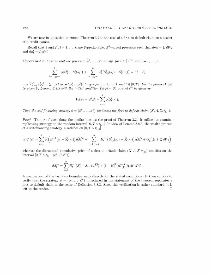
122 CHAPTER 3. HAZARD PROCESS APPROACH
We are now in a position to extend Theorem 3.2 to the case of a first-to-default claim on a basketof n credit names.
Recall that ξ and ζl, l = 1, . . . , k are F-predictable, Rd-valued processes such that dmt = ξt dWt
and dnlt = ζl
t dWt.
Theorem 3.3 Assume that the processes φ1, . . . , φn satisfy, for t ∈ [0, T ] and i = 1, . . . , n
k∑
l=1, jl=i
φlt
(δlt − Sl
t(κl))
+k∑
l=1, jl 6=i
φlt
(Sl
t|i(κl)− Slt(κl)
)= Zi
t − St
and∑k
l=1 φltζ
lt = ξt. Let us set φi
t = φi(t ∧ τ(1)) for i = 1, . . . , k and t ∈ [0, T ]. Let the process V (φ)be given by Lemma 3.8.3 with the initial condition V0(φ) = Sc
0 and let φ0 be given by
Vt(φ) = φ0t Bt +
k∑
l=1
φltS
lt(κl).
Then the self-financing strategy φ = (φ0, . . . , φk) replicates the first-to-default claim (X, A, Z, τ(1)).
Proof. The proof goes along the similar lines as the proof of Theorem 3.2. It suffices to examinereplicating strategy on the random interval [0, T ∧ τ(1)]. In view of Lemma 3.8.3, the wealth processof a self-financing strategy φ satisfies on [0, T ∧ τ(1)]
dV ∗t (φ) =
k∑
l=1
φlt
(B−1
t
(δlt − Sl
t(κl))dM jl
t +n∑
j=1 ,j 6=jl
B−1t
(Sl
t|j(κl)− Slt(κl)
)dM j
t + G−1(1)(t; t)ζ
lt dWt
)
whereas the discounted cumulative price of a first-to-default claim (X, A, Z, τ(1)) satisfies on theinterval [0, T ∧ τ(1)] (cf. (3.87))
dSc∗t =
n∑
i=1
B−1t (Zi
t − St−) dM it + (1−H
(1)t )G−1
(1)(t; t)ξt dWt.
A comparison of the last two formulae leads directly to the stated conditions. It then suffices toverify that the strategy φ = (φ0, . . . , φk) introduced in the statement of the theorem replicates afirst-to-default claim in the sense of Definition 3.8.3. Since this verification is rather standard, it isleft to the reader. ¤
Chapter 4
Hedging of Defaultable Claims
In this chapter, we shall study hedging strategies for credit derivatives under assumption that someprimary defaultable (as well as non-defaultable) assets are traded, and thus they can be used inreplication of non-traded contingent claims. We follow here the paper by Bielecki et al. [8].
4.1 Semimartingale Model with a Common Default
In what follows, we fix a finite horizon date T > 0. For the purpose of this chapter, it is enough toformally define a generic defaultable claim through the following definition.
Definition 4.1.1 A defaultable claim with maturity date T is represented by a triplet (X, Z, τ),where:(i) the default time τ specifies the random time of default, and thus also the default events τ ≤ tfor every t ∈ [0, T ],(ii) the promised payoff X ∈ FT represents the random payoff received by the owner of the claimat time T, provided that there was no default prior to or at time T ; the actual payoff at time Tassociated with X thus equals X1T<τ,(iii) the F-adapted recovery process Z specifies the recovery payoff Zτ received by the owner of aclaim at time of default (or at maturity), provided that the default occurred prior to or at maturitydate T .
In practice, hedging of a credit derivative after default time is usually of minor interest. Also, ina model with a single default time, hedging after default reduces to replication of a non-defaultableclaim. It is thus natural to define the replication of a defaultable claim in the following way.
Definition 4.1.2 We say that a self-financing strategy φ replicates a defaultable claim (X, Z, τ) ifits wealth process V (φ) satisfies VT (φ)1T<τ = X1T<τ and Vτ (φ)1T≥τ = Zτ1T≥τ.
When dealing with replicating strategies, in the sense of Definition 4.1.2, we will always assume,without loss of generality, that the components of the process φ are F-predictable processes.
4.1.1 Dynamics of Asset Prices
We assume that we are given a probability space (Ω,G,P) endowed with a (possibly multi-dimensional)standard Brownian motion W and a random time τ admitting the F-intensity γ under P, where Fis the filtration generated by W .
123

124 CHAPTER 4. HEDGING OF DEFAULTABLE CLAIMS
Since the default time is assumed to admit the F-intensity, it is not an F-stopping time. Indeed,any stopping time with respect to a Brownian filtration is known to be predictable.
We interpret τ as the common default time for all defaultable assets in our model. For simplicity,we assume that only three primary assets are traded in the market, and the dynamics under thehistorical probability P of their prices are, for i = 1, 2, 3 and t ∈ [0, T ],
dY it = Y i
t−(µi,t dt + σi,t dWt + κi,t dMt
), (4.1)
where Mt = Ht −∫ t
0(1−Hs)γs ds is a martingale, or equivalently,
dY it = Y i
t−((µi,t − κi,tγt1t<τ) dt + σi,t dWt + κi,t dHt
). (4.2)
The processes (µi, σi, κi) = (µi,t, σi,t, κi,t, t ∈ R+), i = 1, 2, 3, are assumed to be G-adapted, whereG = F ∨ H. In addition, we assume that κi ≥ −1 for any i = 1, 2, 3, so that Y i are nonnegativeprocesses, and they are strictly positive prior to τ . Note that, in the case of constant coefficients wehave that
Y it = Y i
0 eµiteσiWt−σ2i t/2e−κiγi(t∧τ)(1 + κi)Ht .
According to Definition 4.1.2, replication refers to the behavior of the wealth process V (φ) onthe random interval [[0, τ ∧ T ]] only. Therefore, for the purpose of replication of defaultable claimsof the form (X, Z, τ), it is sufficient to consider prices of primary assets stopped at τ ∧ T . Thisimplies that instead of dealing with G-adapted coefficients in (4.1), it suffices to focus on F-adaptedcoefficients of stopped price processes. However, for the sake of completeness, we shall also deal withT -maturity claims of the form Y = G(Y 1
T , Y 2T , Y 3
T ,HT ) (see Section 4.4 below).
Pre-Default Values
As will become clear in what follows, when dealing with defaultable claims of the form (X,Z, τ), wewill be mainly concerned with the so-called pre-default prices. The pre-default price Y i of the ithasset is an F-adapted, continuous process, given by the equation, for i = 1, 2, 3 and t ∈ [0, T ],
dY it = Y i
t
((µi,t − κi,tγt) dt + σi,t dWt
)(4.3)
with Y i0 = Y i
0 . Put another way, Y i is the unique F-predictable process such that Y it 1t≤τ =
Y it 1t≤τ for t ∈ R+. When dealing with the pre-default prices, we may and do assume, without
loss of generality, that the processes µi, σi and κi are F-predictable.
It is worth stressing that the historically observed drift coefficient equals µi,t − κi,tγt, ratherthan µi,t. The drift coefficient denoted by µi,t is already credit-risk adjusted in the sense of ourmodel, and it is not directly observed. This convention was chosen here for the sake of simplicity ofnotation. It also lends itself to the following intuitive interpretation: if φi is the number of units ofthe ith asset held in our portfolio at time t then the gains/losses from trades in this asset, prior todefault time, can be represented by the differential
φit dY i
t = φitY
it
(µi,t dt + σi,t dWt
)− φitY
it κi,tγt dt.
The last term may be here separated, and formally treated as an effect of continuously paid dividendsat the dividend rate κi,tγt. However, this interpretation may be misleading, since this quantity is notdirectly observed. In fact, the estimation of the drift coefficient in dynamics (4.3) is not practical.
Still, if this formal interpretation is adopted, it is sometimes possible make use of the standardresults concerning the valuation of derivatives of dividend-paying assets. It is, of course, a delicateissue how to separate in practice both components of the drift coefficient. We shall argue belowthat although the dividend-based approach is formally correct, a more pertinent and simpler way ofdealing with hedging relies on the assumption that only the effective drift µi,t− κi,tγt is observable.In practical approach to hedging, the values of drift coefficients in dynamics of asset prices play noessential role, so that they are not considered to be market observables.

4.1. TRADING STRATEGIES 125
Market Observables
To summarize, we assume throughout that the market observables are: the pre-default market pricesof primary assets, their volatilities and correlations, as well as the jump coefficients κi,t (the financialinterpretation of jump coefficients is examined in the next subsection). To summarize, we postulatethat under the statistical probability P we have
dY it = Y i
t−(µi,t dt + σi,t dWt + κi,t dHt
)(4.4)
where the drift terms µi,t are not observed, but we can observe the volatilities σi,t (and thus the assetscorrelations) and we have an a priori assessment of jump coefficients κi,t. In this general setup, themost natural assumption is that the dimension of a driving Brownian motion W equals the numberof tradable assets. However, for the sake of simplicity of presentation, we shall frequently assumethat W is one-dimensional. One of our goals will be to derive closed-form solutions for replicatingstrategies for derivative securities in terms of market observables only (whenever replication ofa given claim is actually feasible). To achieve this goal, we shall combine a general theory ofhedging defaultable claims within a continuous semimartingale setup, with a judicious specificationof particular models with deterministic volatilities and correlations.
Recovery Schemes
It is clear that the sample paths of price processes Y i are continuous, except for a possible discon-tinuity at time τ . Specifically, we have that
∆Y iτ := Y i
τ − Y iτ− = κi,τY i
τ−,
so that Y iτ = Y i
τ−(1 + κi,τ ) = Y iτ−(1 + κi,τ ).
A primary asset Y i is termed a default-free asset (defaultable asset, respectively) if κi = 0 (κi 6= 0,respectively). In the special case when κi = −1, we say that a defaultable asset Y i is subject to atotal default, since its price drops to zero at time τ and stays there forever. Such an asset ceases toexist after default, in the sense that it is no longer traded after default. This feature makes the caseof a total default quite different from other cases, as we shall see in our study below.
In market practice, it is common for a credit derivative to deliver a positive recovery (for instance,a protection payment) in case of default. Formally, the value of this recovery at default is determinedas the value of some underlying process, that is, it is equal to the value at time τ of some F-adaptedrecovery process Z.
For example, the process Z can be equal to δ, where δ is a constant, or to g(t, δYt) where g is adeterministic function and (Yt, t ∈ R+) is the price process of some default-free asset. Typically, therecovery is paid at default time, but it may also happen that it is postponed to the maturity date.
Let us observe that the case where a defaultable asset Y i pays a pre-determined recovery atdefault is covered by our setup defined in (4.1). For instance, the case of a constant recovery payoffδi ≥ 0 at default time τ corresponds to the process κi,t = δi(Y i
t−)−1 − 1. Under this convention, theprice Y i is governed under P by the SDE
dY it = Y i
t−(µi,t dt + σi,t dWt + (δi(Y i
t−)−1 − 1) dMt
). (4.5)
If the recovery is proportional to the pre-default value Y iτ−, and is paid at default time τ (this scheme
is known as the fractional recovery of market value), we have κi,t = δi − 1 and
dY it = Y i
t−(µi,t dt + σi,t dWt + (δi − 1) dMt
). (4.6)
Throughout this chapter, we write∫ ·0
to denote∫]0,·].

126 CHAPTER 4. HEDGING OF DEFAULTABLE CLAIMS
4.2 Trading Strategies in a Semimartingale Set-up
We consider trading within the time interval [0, T ] for some finite horizon date T > 0. For thesake of expositional clarity, we restrict our attention to the case where only three primary assets aretraded. The general case of k traded assets was examined by Bielecki et al. [7, 9].
In this section, we consider a fairly general setup. In particular, processes Y i, i = 1, 2, 3, areassumed to be nonnegative semi-martingales on a probability space (Ω,G,P) endowed with somefiltration G. We assume that they represent spot prices of traded assets in our model of the financialmarket. Neither the existence of a savings account, nor the market completeness are assumed, ingeneral.
Our goal is to characterize contingent claims which are hedgeable, in the sense that they canbe replicated by continuously rebalanced portfolios consisting of primary assets. Here, by a con-tingent claim we mean an arbitrary GT -measurable random variable. We work under the standardassumptions of a frictionless market.
4.2.1 Unconstrained Strategies
Let φ = (φ1, φ2, φ3) be a trading strategy; in particular, each process φi is predictable with respectto the filtration G. The wealth of φ equals
Vt(φ) =3∑
i=1
φitY
it , ∀ t ∈ [0, T ],
and a trading strategy φ is said to be self-financing if
Vt(φ) = V0(φ) +3∑
i=1
∫ t
0
φiu dY i
u, ∀ t ∈ [0, T ].
Let Φ stand for the class of all self-financing trading strategies. We shall first prove that a self-financing strategy is determined by its initial wealth and the two components φ2, φ3. To this end,we postulate that the price of Y 1 follows a strictly positive process, and we choose Y 1 as a numeraireasset. We shall now analyze the relative values:
V 1t (φ) := Vt(φ)(Y 1
t )−1, Y i,1t := Y i
t (Y 1t )−1.
Lemma 4.2.1 (i) For any φ ∈ Φ, we have
V 1t (φ) = V 1
0 (φ) +3∑
i=2
∫ t
0
φiu dY i,1
u , ∀ t ∈ [0, T ].
(ii) Conversely, let X be a GT -measurable random variable, and let us assume that there exists x ∈ Rand G-predictable processes φi, i = 2, 3 such that
X = Y 1T
(x +
3∑
i=2
∫ T
0
φiu dY i,1
u
). (4.7)
Then there exists a G-predictable process φ1 such that the strategy φ = (φ1, φ2, φ3) is self-financingand replicates X. Moreover, the wealth process of φ (i.e. the time-t price of X) satisfies Vt(φ) =V 1
t Y 1t , where
V 1t = x +
3∑
i=2
∫ t
0
φiu dY i,1
u , ∀ t ∈ [0, T ]. (4.8)

4.2. TRADING STRATEGIES 127
Proof. In the case of continuous semimartingales, (it is a well-known result; for discontinuousprocesses, the proof is not much different. We reproduce it here for the reader’s convenience.
Let us first introduce some notation. As usual, [X,Y ] stands for the quadratic covariation of thetwo semi-martingales X and Y , as defined by the integration by parts formula:
XtYt = X0Y0 +∫ t
0
Xu− dYu +∫ t
0
Yu− dXu + [X,Y ]t.
For any cadlag (i.e., RCLL) process Y , we denote by ∆Yt = Yt − Yt− the size of the jump at timet. Let V = V (φ) be the value of a self-financing strategy, and let V 1 = V 1(φ) = V (φ)(Y 1)−1 be itsvalue relative to the numeraire Y 1. The integration by parts formula yields
dV 1t = Vt−d(Y 1
t )−1 + (Y 1t−)−1dVt + d[(Y 1)−1, V ]t.
From the self-financing condition, we have dVt =∑3
i=1 φit dY i
t . Hence, using elementary rules tocompute the quadratic covariation [X, Y ] of the two semi-martingales X,Y , we obtain
dV 1t = φ1
t Y1t− d(Y 1
t )−1 + φ2t Y
2t− d(Y 1
t )−1 + φ3t Y
3t− d(Y 1
t )−1
+ (Y 1t−)−1φ1
t dY 1t + (Y 1
t−)−1φ2t dY 1
t + (Y 1t−)−1φ3
t dY 1t
+ φ1t d[(Y 1)−1, Y 1]t + φ2
t d[(Y 1)−1, Y 2]t + φ3t d[(Y 1)−1, Y 1]t
= φ1t
(Y 1
t− d(Y 1t )−1 + (Y 1
t−)−1 dY 1t + d[(Y 1)−1, Y 1]t
)
+ φ2t
(Y 2
t− d(Y 1t )−1 + (Y 1
t−)−1 dY 1t− + d[(Y 1)−1, Y 2]t
)
+ φ3t
(Y 3
t− d(Y 1t )−1 + (Y 1
t−)−1 dY 1t− + d[(Y 1)−1, Y 3]t
).
We now observe that
Y 1t− d(Y 1
t )−1 + (Y 1t−)−1 dY 1
t + d[(Y 1)−1, Y 1]t = d(Y 1t (Y 1
t )−1) = 0
andY i
t− d(Y 1t )−1 + (Y 1
t−)−1 dY it + d[(Y 1)−1, Y i]t = d((Y 1
t )−1Y it ).
Consequently,dV 1
t = φ2t dY 2,1
t + φ3t dY 3,1
t ,
as was claimed in part (i). We now proceed to the proof of part (ii). We assume that (4.7) holds forsome constant x and processes φ2, φ3, and we define the process V 1 by setting (cf. (4.8))
V 1t = x +
3∑
i=2
∫ t
0
φiu dY i,1
u , ∀ t ∈ [0, T ].
Next, we define the process φ1 as follows:
φ1t = V 1
t −3∑
i=2
φitY
i,1t = (Y 1
t )−1(Vt −
3∑
i=2
φitY
it
),
where Vt = V 1t Y 1
t . Since
dV 1t =
3∑
i=2
φit dY i,1
t ,
we obtain
dVt = d(V 1t Y 1
t ) = V 1t−dY 1
t + Y 1t−dV 1
t + d[Y 1, V 1]t
= V 1t−dY 1
t +3∑
i=2
φit
(Y 1
t− dY i,1t + d[Y 1, Y i,1]t
).

128 CHAPTER 4. HEDGING OF DEFAULTABLE CLAIMS
From the equality
dY it = d(Y i,1
t Y 1t ) = Y i,1
t− dY 1t + Y 1
t−dY i,1t + d[Y 1, Y i,1]t,
it follows that
dVt = V 1t−dY 1
t +3∑
i=2
φit
(dY i
t − Y i,1t− dY 1
t
)=
(V 1
t− −3∑
i=2
φitY
i,1t−
)dY 1
t +3∑
i=2
φit dY i
t ,
and our aim is to prove that dVt =∑3
i=1 φit dY i
t . The last equality holds if
φ1t = V 1
t −3∑
i=2
φitY
i,1t = V 1
t− −3∑
i=2
φitY
i,1t− , (4.9)
i.e., if ∆V 1t =
∑3i=2 φi
t∆Y i,1t , which is the case from the definition (4.8) of V 1. Note also that from
the second equality in (4.9) it follows that the process φ1 is indeed G-predictable. Finally, the wealthprocess of φ satisfies Vt(φ) = V 1
t Y 1t for every t ∈ [0, T ], and thus VT (φ) = X. ¤
We say that a self-financing strategy φ replicates a claim X ∈ GT if
X =3∑
i=1
φiT Y i
T = VT (φ),
or equivalently,
X = V0(φ) +3∑
i=1
∫ T
0
φit dY i
t .
Suppose that there exists an EMM for some choice of a numeraire asset, and let us restrict ourattention to the class of all admissible trading strategies, so that our model is arbitrage-free.
Assume that a claim X can be replicated by some admissible trading strategy, so that it isattainable (or hedgeable). Then, by definition, the arbitrage price at time t of X, denoted as πt(X),equals Vt(φ) for any admissible trading strategy φ that replicates X.
In the context of Lemma 4.2.1, it is natural to choose as an EMM a probability measure Q1
equivalent to P on (Ω,GT ) and such that the prices Y i,1, i = 2, 3, are G-martingales under Q1. If acontingent claim X is hedgeable, then its arbitrage price satisfies
πt(X) = Y 1t EQ1(X(Y 1
T )−1 | Gt).
We emphasize that even if an EMM Q1 is not unique, the price of any hedgeable claim X is givenby this conditional expectation. That is to say, in case of a hedgeable claim these conditionalexpectations under various equivalent martingale measures coincide.
In the special case where Y 1t = B(t, T ) is the price of a default-free zero-coupon bond with
maturity T (abbreviated as ZCB in what follows), Q1 is called T -forward martingale measure,and it is denoted by QT . Since B(T, T ) = 1, the price of any hedgeable claim X now equalsπt(X) = B(t, T )EQT
(X | Gt).
4.2.2 Constrained Strategies
In this section, we make an additional assumption that the price process Y 3 is strictly positive. Letφ = (φ1, φ2, φ3) be a self-financing trading strategy satisfying the following constraint:
2∑
i=1
φitY
it− = Zt, ∀ t ∈ [0, T ], (4.10)

4.2. TRADING STRATEGIES 129
for a predetermined, G-predictable process Z. In the financial interpretation, equality (4.10) meansthat a portfolio φ is rebalanced in such a way that the total wealth invested in assets Y 1, Y 2 matchesa predetermined stochastic process Z. For this reason, the constraint given by (4.10) is referred toas the balance condition.
Our first goal is to extend part (i) in Lemma 4.2.1 to the case of constrained strategies. LetΦ(Z) stand for the class of all (admissible) self-financing trading strategies satisfying the balancecondition (4.10). They will be sometimes referred to as constrained strategies. Since any strategyφ ∈ Φ(Z) is self-financing, from dVt(φ) =
∑3i=1 φi
t dY it , we obtain
∆Vt(φ) =3∑
i=1
φit∆Y i
t = Vt(φ)−3∑
i=1
φitY
it−.
By combining this equality with (4.10), we deduce that
Vt−(φ) =3∑
i=1
φitY
it− = Zt + φ3
t Yit−.
Let us writeY i,3
t = Y it (Y 3
t )−1, Z3t = Zt(Y 3
t )−1.
The following result extends Lemma 1.7 in Bielecki et al. [4] from the case of continuous semi-martingales to the general case (see also [7, 9]). It is apparent from Proposition 4.2.1 that thewealth process V (φ) of a strategy φ ∈ Φ(Z) depends only on a single component of φ, namely, φ2.
Proposition 4.2.1 The relative wealth V 3t (φ) = Vt(φ)(Y 3
t )−1 of any trading strategy φ ∈ Φ(Z)satisfies
V 3t (φ) = V 3
0 (φ) +∫ t
0
φ2u
(dY 2,3
u − Y 2,3u−
Y 1,3u−
dY 1,3u
)+
∫ t
0
Z3u
Y 1,3u−
dY 1,3u . (4.11)
Proof. Let us consider discounted values of price processes Y 1, Y 2, Y 3, with Y 3 taken as a numeraireasset. By virtue of part (i) in Lemma 4.2.1, we thus have
V 3t (φ) = V 3
0 (φ) +2∑
i=1
∫ t
0
φiu dY i,3
u . (4.12)
The balance condition (4.10) implies that
2∑
i=1
φitY
i,3t− = Z3
t ,
and thusφ1
t = (Y 1,3t− )−1
(Z3
t − φ2t Y
2,3t−
). (4.13)
By inserting (4.13) into (4.12), we arrive at the desired formula (4.11). ¤The next result will prove particularly useful for deriving replicating strategies for defaultable
claims.
Proposition 4.2.2 Let a GT -measurable random variable X represent a contingent claim that settlesat time T . We set
dY ∗t = dY 2,3
t − Y 2,3t−
Y 1,3t−
dY 1,3t = dY 2,3
t − Y 2,1t− dY 1,3
t , (4.14)
130 CHAPTER 4. HEDGING OF DEFAULTABLE CLAIMS
where, by convention, Y ∗0 = 0. Assume that there exists a G-predictable process φ2, such that
X = Y 3T
(x +
∫ T
0
φ2t dY ∗
t +∫ T
0
Z3t
Y 1,3t−
dY 1,3t
). (4.15)
Then there exist G-predictable processes φ1 and φ3 such that the strategy φ = (φ1, φ2, φ3) belongs toΦ(Z) and replicates X. The wealth process of φ equals, for every t ∈ [0, T ],
Vt(φ) = Y 3t
(x +
∫ t
0
φ2u dY ∗
u +∫ t
0
Z3u
Y 1,3u−
dY 1,3u
). (4.16)
Proof. As expected, we first set (note that the process φ1 is a G-predictable process)
φ1t =
1Y 1
t−
(Zt − φ2
t Y2t−
)(4.17)
and
V 3t = x +
∫ t
0
φ2u dY ∗
u +∫ t
0
Z3u
Y 1,3u−
dY 1,3u .
Arguing along the same lines as in the proof of Proposition 4.2.1, we obtain
V 3t = V 3
0 +2∑
i=1
∫ t
0
φiu dY i,3
u .
Now, we define
φ3t = V 3
t −2∑
i=1
φitY
i,3t = (Y 3
t )−1(Vt −
2∑
i=1
φitY
it
),
where Vt = V 3t Y 3
t . As in the proof of Lemma 4.2.1, we check that
φ3t = V 3
t− −2∑
i=1
φitY
i,3t− ,
and thus the process φ3 is G-predictable. It is clear that the strategy φ = (φ1, φ2, φ3) is self-financingand its wealth process satisfies Vt(φ) = Vt for every t ∈ [0, T ]. In particular, VT (φ) = X, so that φreplicates X. Finally, equality (4.17) implies (4.10), and thus φ belongs to the class Φ(Z). ¤
Note that equality (4.15) is a necessary (by Lemma 4.2.1) and sufficient (by Proposition 4.2.2)condition for the existence of a constrained strategy that replicates a given contingent claim X.
Synthetic Asset
Let us take Z = 0, so that φ ∈ Φ(0). Then the balance condition becomes∑2
i=1 φitY
it− = 0, and
formula (4.11) reduces to
dV 3t (φ) = φ2
t
(dY 2,3
t − Y 2,3t−
Y 1,3t−
dY 1,3t
). (4.18)
The process Y 2 = Y 3Y ∗, where Y ∗ is defined in (4.14) is called a synthetic asset. It correspondsto a particular self-financing portfolio, with the long position in Y 2 and the short position of Y 2,1
t−number of shares of Y 1, and suitably re-balanced positions in the third asset so that the portfolio isself-financing, as in Lemma 4.2.1.
It can be shown (see Bielecki et al. [7, 9]) that trading in primary assets Y 1, Y 2, Y 3 is formallyequivalent to trading in assets Y 1, Y 2, Y 3. This observation supports the name synthetic assetattributed to the process Y 2. Note, however, that the synthetic asset process may take negativevalues.

4.2. TRADING STRATEGIES 131
Case of Continuous Asset Prices
In the case of continuous asset prices, the relative price Y ∗ = Y 2(Y 3)−1 of the synthetic asset can begiven an alternative representation, as the following result shows. Recall that the predictable bracketof the two continuous semi-martingales X and Y , denoted as 〈X,Y 〉, coincides with their quadraticcovariation [X,Y ].
Proposition 4.2.3 Assume that the price processes Y 1 and Y 2 are continuous. Then the relativeprice of the synthetic asset satisfies
Y ∗t =
∫ t
0
(Y 3,1u )−1eαu dYu,
where Yt := Y 2,1t e−αt and
αt := 〈ln Y 2,1, ln Y 3,1〉t =∫ t
0
(Y 2,1u )−1(Y 3,1
u )−1 d〈Y 2,1, Y 3,1〉u. (4.19)
In terms of the auxiliary process Y , formula (4.11) becomes
V 3t (φ) = V 3
0 (φ) +∫ t
0
φu dYu +∫ t
0
Z3u
Y 1,3u−
dY 1,3u , (4.20)
where φt = φ2t (Y
3,1t )−1eαt .
Proof. It suffices to give the proof for Z = 0. The proof relies on the integration by parts formulastating that for any two continuous semi-martingales, say X and Y , we have
Y −1t
(dXt − Y −1
t d〈X, Y 〉t)
= d(XtY−1t )−Xt dY −1
t ,
provided that Y is strictly positive. An application of this formula to processes X = Y 2,1 andY = Y 3,1 leads to
(Y 3,1t )−1
(dY 2,1
t − (Y 3,1t )−1d〈Y 2,1, Y 3,1〉t
)= d(Y 2,1
t (Y 3,1t )−1)− Y 2,1
t d(Y 3,1)−1t .
The relative wealth V 3t (φ) = Vt(φ)(Y 3
t )−1 of a strategy φ ∈ Φ(0) satisfies
V 3t (φ) = V 3
0 (φ) +∫ t
0
φ2u dY ∗
u
= V 30 (φ) +
∫ t
0
φ2u(Y 3,1
u )−1eαu dYu,
= V 30 (φ) +
∫ t
0
φu dYu
where we denote φt = φ2t (Y
3,1t )−1eαt .
Remark 4.2.1 The financial interpretation of the auxiliary process Y will be studied below. Letus only observe here that if Y ∗ is a local martingale under some probability Q then Y is a Q-localmartingale (and vice versa, if Y is a Q-local martingale under some probability Q then Y ∗ is aQ-local martingale). Nevertheless, for the reader’s convenience, we shall use two symbols Q and Q,since this equivalence holds for continuous processes only.
It is thus worth stressing that we will apply Proposition 4.2.3 to pre-default values of assets,rather than directly to asset prices, within the setup of a semimartingale model with a commondefault, as described in Section 4.1.1. In this model, the asset prices may have discontinuities, buttheir pre-default values follow continuous processes.

132 CHAPTER 4. HEDGING OF DEFAULTABLE CLAIMS
4.3 Martingale Approach to Valuation and Hedging
Our goal is to derive quasi-explicit conditions for replicating strategies for a defaultable claim in afairly general setup introduced in Section 4.1.1. In this section, we only deal with trading strategiesbased on the reference filtration F and the underlying price processes (that is, prices of default-freeassets and pre-default values of defaultable assets) are assumed to be continuous. Therefore, ourarguments will hinge on Proposition 4.2.3, rather than on a more general Proposition 4.2.1. Weshall also adapt Proposition 4.2.2 to our current purposes. To simplify the presentation, we makea standing assumption that all coefficient processes are such that the SDEs appearing below admitunique strong solutions, and all stochastic exponentials (used as Radon-Nikodym derivatives) aretrue martingales under respective probabilities.
4.3.1 Defaultable Asset with Total Default
In this section, we shall examine in some detail a particular model where the two assets, Y 1 and Y 2,are default-free and satisfy
dY it = Y i
t
(µi,t dt + σi,t dWt
), i = 1, 2,
where W is a one-dimensional Brownian motion. The third asset is a defaultable asset with totaldefault, so that
dY 3t = Y 3
t−(µ3,t dt + σ3,t dWt − dMt
).
Since we will be interested in replicating strategies in the sense of Definition 4.1.2, we may and doassume, without loss of generality, that the coefficients µi,t, σi,t, i = 1, 2, are F-predictable, ratherthan G-predictable. Recall that, in general, there exist F-predictable processes µ3 and σ3 such that
µ3,t1t≤τ = µ3,t1t≤τ, σ3,t1t≤τ = σ3,t1t≤τ. (4.21)
We assume throughout that Y i0 > 0 for every i, so that the price processes Y 1, Y 2 are strictly
positive, and the process Y 3 is nonnegative, and has strictly positive pre-default value.
Default-Free Market
It is natural to postulate that the default-free market with the two traded assets, Y 1 and Y 2,is arbitrage-free. More precisely, we choose Y 1 as a numeraire, and we require that there exists aprobability measure P1, equivalent to P on (Ω,FT ), and such that the process Y 2,1 is a P1-martingale.The dynamics of processes (Y 1)−1 and Y 2,1 are
d(Y 1t )−1 = (Y 1
t )−1((σ2
1,t − µ1,t) dt− σ1,t dWt
), (4.22)
anddY 2,1
t = Y 2,1t
((µ2,t − µ1,t + σ1,t(σ1,t − σ2,t)) dt + (σ2,t − σ1,t) dWt
),
respectively. Hence the necessary condition for the existence of an EMM P1 is the inclusion A ⊆ B,where A = (t, ω) ∈ [0, T ]×Ω : σ1,t(ω) = σ2,t(ω) and B = (t, ω) ∈ [0, T ]×Ω : µ1,t(ω) = µ2,t(ω).The necessary and sufficient condition for the existence and uniqueness of an EMM P1 reads
EPET
(∫ ·
0
θu dWu
)= 1 (4.23)
where the process θ is given by the formula (by convention, 0/0 = 0)
θt = σ1,t − µ1,t − µ2,t
σ1,t − σ2,t, ∀ t ∈ [0, T ]. (4.24)
Note that in the case of constant coefficients, if σ1 = σ2 then the model is arbitrage-free only in thetrivial case when µ2 = µ1.
4.3. MARTINGALE APPROACH 133
Remark 4.3.1 Since the martingale measure P1 is unique, the default-free model (Y 1, Y 2) is com-plete. However, this is not a necessary assumption and thus it can be relaxed. As we shall seein what follows, it is typically more natural to assume that the driving Brownian motion W ismulti-dimensional.
Arbitrage-Free Property
Let us now consider also a defaultable asset Y 3. Our goal is now to find a martingale measure Q1 (ifit exists) for relative prices Y 2,1 and Y 3,1. Recall that we postulate that the hypothesis (H) holdsunder P for filtrations F and G = F ∨H. The dynamics of Y 3,1 under P are
dY 3,1t = Y 3,1
t−(
µ3,t − µ1,t + σ1,t(σ1,t − σ3,t))dt + (σ3,t − σ1,t) dWt − dMt
.
Let Q1 be any probability measure equivalent to P on (Ω,GT ), and let η be the associatedRadon-Nikodym density process, so that
dQ1 | Gt = ηt dP | Gt , (4.25)
where the process η satisfiesdηt = ηt−(θt dWt + ζt dMt) (4.26)
for some G-predictable processes θ and ζ, and η is a G-martingale under P.
From Girsanov’s theorem, the processes W and M , given by
Wt = Wt −∫ t
0
θu du, Mt = Mt −∫ t
0
1u<τγuζu du, (4.27)
are G-martingales under Q1. To ensure that Y 2,1 is a Q1-martingale, we postulate that (4.23) and(4.24) are valid. Consequently, for the process Y 3,1 to be a Q1-martingale, it is necessary andsufficient that ζ satisfies
γtζt = µ3,t − µ1,t − µ1,t − µ2,t
σ1,t − σ2,t(σ3,t − σ1,t).
To ensure that Q1 is a probability measure equivalent to P, we require that ζt > −1. The uniquemartingale measure Q1 is then given by the formula (4.25) where η solves (4.26), so that
ηt = Et
(∫ ·
0
θu dWu
)Et
(∫ ·
0
ζu dMu
).
We are in a position to formulate the following result.
Proposition 4.3.1 Assume that the process θ given by (4.24) satisfies (4.23), and
ζt =1γt
(µ3,t − µ1,t − µ1,t − µ2,t
σ1,t − σ2,t(σ3,t − σ1,t)
)> −1. (4.28)
Then the model M = (Y 1, Y 2, Y 3; Φ) is arbitrage-free and complete. The dynamics of relative pricesunder the unique martingale measure Q1 are
dY 2,1t = Y 2,1
t (σ2,t − σ1,t) dWt,
dY 3,1t = Y 3,1
t−((σ3,t − σ1,t) dWt − dMt
).
Since the coefficients µi,t, σi,t, i = 1, 2, are F-adapted, the process W is an F-martingale (hence,a Brownian motion) under Q1. Therefore, by virtue of Proposition 3.5.1, the hypothesis (H) holdsunder Q1, and the F-intensity of default under Q1 equals
γt = γt(1 + ζt) = γt +(
µ3,t − µ1,t − µ1,t − µ2,t
σ1,t − σ2,t(σ3,t − σ1,t)
).
134 CHAPTER 4. HEDGING OF DEFAULTABLE CLAIMS
Example 4.3.1 We present an example where the condition (4.28) does not hold, and thus arbitrageopportunities arise. Assume that the coefficients are constant and satisfy: µ1 = µ2 = σ1 = 0, µ3 <−γ for a constant default intensity γ > 0. Then
Y 3t = 1t<τY 3
0 exp(
σ3Wt − 12σ2
3t + (µ3 + γ)t)≤ Y 3
0 exp(
σ3Wt − 12σ2
3t
)= Vt(φ),
where V (φ) represents the wealth of a self-financing strategy (φ1, φ2, 0) with φ2 = σ3σ2
. Hence thearbitrage strategy would be to sell the asset Y 3, and to follow the strategy φ.
Remark 4.3.2 Let us stress once again, that the existence of an EMM is a necessary condition forviability of a financial model, but the uniqueness of an EMM is not always a convenient conditionto impose on a model. In fact, when constructing a model, we should be mostly concerned withits flexibility and ability to reflect the pertinent risk factors, rather than with its mathematicalcompleteness. In the present context, it is natural to postulate that the dimension of the underlyingBrownian motion equals the number of tradeable risky assets. In addition, each particular modelshould be tailored to provide intuitive and handy solutions for a predetermined family of contingentclaims that will be priced and hedged within its framework.
Hedging a Survival Claim
We first focus on replication of a survival claim (X, 0, τ), that is, a defaultable claim represented bythe terminal payoff X1T<τ, where X is an FT -measurable random variable. For the moment, wemaintain the simplifying assumption that W is one-dimensional. As we shall see in what follows,it may lead to certain pathological features of a model. If, on the contrary, the driving noise ismulti-dimensional, most of the analysis remains valid, except that the model completeness is nolonger ensured, in general.
Recall that Y 3 stands for the pre-default price of Y 3, defined as (see (4.3))
dY 3t = Y 3
t
((µ3,t + γt) dt + σ3,t dWt
)(4.29)
with Y 30 = Y 3
0 . This strictly positive, continuous, F-adapted process enjoys the property that Y 3t =
1t<τY 3t . Let us denote the pre-default values in the numeraire Y 3 by Y i,3
t = Y it (Y 3
t )−1, i = 1, 2,and let us introduce the pre-default relative price Y ∗ of the synthetic asset Y 2 by setting
dY ∗t := dY 2,3
t − Y 2,3t
Y 1,3t
dY 1,3t = Y 2,3
t
((µ2,t − µ1,t + σ3,t(σ1,t − σ2,t)
)dt + (σ2,t − σ1,t) dWt
),
and let us assume that σ1,t − σ2,t 6= 0. It is also useful to note that the process Y , defined inProposition 4.2.3, satisfies
dYt = Yt
((µ2,t − µ1,t + σ3,t(σ1,t − σ2,t)
)dt + (σ2,t − σ1,t) dWt
).
We shall show that in the case, where α given by (4.19) is deterministic, the process Y has a nicefinancial interpretation as a credit-risk adjusted forward price of Y 2 relative to Y 1. Therefore, it ismore convenient to work with the process Y ∗ when dealing with the general case, but to use theprocess Y when analyzing a model with deterministic volatilities.
Consider an F-predictable self-financing strategy φ satisfying the balance condition φ1t Y
1t +
φ2t Y
2t = 0, and the corresponding wealth process
Vt(φ) :=3∑
i=1
φitY
it = φ3
t Y3t .
4.3. MARTINGALE APPROACH 135
Let Vt(φ) := φ3t Y
3t . Since the process V (φ) is F-adapted, we see that this is the pre-default price
process of the portfolio φ, that is, we have 1τ>tVt(φ) = 1τ>tVt(φ); we shall call this process thepre-default wealth of φ. Consequently, the process V 3
t (φ) := Vt(φ)(Y 3t )−1 = φ3
t is termed the relativepre-default wealth.
Using Proposition 4.2.1, with suitably modified notation, we find that the F-adapted processV 3(φ) satisfies, for every t ∈ [0, T ],
V 3t (φ) = V 3
0 (φ) +∫ t
0
φ2u dY ∗
u .
Define a new probability Q∗ on (Ω,FT ) by setting
dQ∗ = η∗T dP,
where dη∗t = η∗t θ∗t dWt, and
θ∗t =µ2,t − µ1,t + σ3,t(σ1,t − σ2,t)
σ1,t − σ2,t. (4.30)
The process Y ∗t , t ∈ [0, T ], is a (local) martingale under Q∗ driven by a Brownian motion. We shall
require that this process is in fact a true martingale; a sufficient condition for this is that∫ T
0
EQ∗(Y 2,3
t (σ2,t − σ1,t))2
dt < ∞.
From the predictable representation theorem, it follows that for any X ∈ FT , such that X(Y 3T )−1 is
square-integrable under Q, there exists a constant x and an F-predictable process φ2 such that
X = Y 3T
(x +
∫ T
0
φ2u dY ∗
u
). (4.31)
We now deduce from Proposition 4.2.2 that there exists a self-financing strategy φ with the pre-default wealth Vt(φ) = Y 3
t V 3t for every t ∈ [0, T ], where we set
V 3t = x +
∫ t
0
φ2u dY ∗
u . (4.32)
Moreover, it satisfies the balance condition φ1t Y
1t + φ2
t Y2t = 0 for every t ∈ [0, T ]. Since clearly
VT (φ) = X, we have that
VT (φ) = φ3T Y 3
T = 1T<τφ3T Y 3
T = 1T<τVT (φ) = 1T<τX,
and thus this strategy replicates the survival claim (X, 0, τ). In fact, we have that Vt(φ) = 0 on therandom interval [[τ, T ]].
Definition 4.3.1 We say that a survival claim (X, 0, τ) is attainable if the process V 3 given by(4.32) is a martingale under Q∗.
The following result is an immediate consequence of (4.31) and (4.32).
Corollary 4.3.1 Let X ∈ FT be such that X(Y 3T )−1 is square-integrable under Q∗. Then the
survival claim (X, 0, τ) is attainable. Moreover, the pre-default price πt(X, 0, τ) of the claim (X, 0, τ)is given by the conditional expectation
πt(X, 0, τ) = Y 3t EQ∗(X(Y 3
T )−1 | Ft), ∀ t ∈ [0, T ]. (4.33)
The process π(X, 0, τ)(Y 3)−1 is an F-martingale under Q.

136 CHAPTER 4. HEDGING OF DEFAULTABLE CLAIMS
Proof. Since X(Y 3T )−1 is square-integrable under Q, we know from the predictable representation
theorem that φ2 in (4.31) is such that EQ∗(∫ T
0(φ2
t )2 d〈Y ∗〉t)
< ∞, so that the process V 3 given by(4.32) is a true martingale under Q. We conclude that (X, 0, τ) is attainable.
Now, let us denote by πt(X, 0, τ) the time-t price of the claim (X, 0, τ). Since φ is a hedgingportfolio for (X, 0, τ) we thus have Vt(φ) = πt(X, 0, τ) for each t ∈ [0, T ]. Consequently,
1τ>tπt(X, 0, τ) = 1τ>tVt(φ) = 1τ>tY 3t EQ∗(V 3
T | Ft)
= 1τ>tY 3t EQ∗(X(Y 3
T )−1 | Ft)
for each t ∈ [0, T ]. This proves equality (4.33). ¤In view of the last result, it is justified to refer to Q as the pricing measure relative to Y 3 for
attainable survival claims.
Remark 4.3.3 It can be proved that there exists a unique absolutely continuous probability mea-sure Q on (Ω,GT ) such that we have
Y 3t EQ
(1τ>TX
Y 3T
∣∣∣Gt
)= 1τ>tY 3
t EQ∗(
X
Y 3T
∣∣∣Ft
).
However, this probability measure is not equivalent to Q, since its Radon-Nikodym density vanishesafter τ (for a related result, see Collin-Dufresne et al. [32]).
Example 4.3.2 We provide here an explicit calculation of the pre-default price of a survival claim.For simplicity, we assume that X = 1, so that the claim represents a defaultable zero-coupon bond.Also, we set γt = γ = const, µi,t = 0, and σi,t = σi, i = 1, 2, 3. Straightforward calculations yieldthe following pricing formula
π0(1, 0, τ) = Y 30 e−(γ+ 1
2 σ23)T .
We see that here the pre-default price π0(1, 0, τ) depends explicitly on the intensity γ, or rather,on the drift term in dynamics of pre-default value of defaultable asset. Indeed, from the practicalviewpoint, the interpretation of the drift coefficient in dynamics of Y 2 as the real-world defaultintensity is questionable, since within our setup the default intensity never appears as an independentvariable, but is merely a component of the drift term in dynamics of pre-default value of Y 3.
Note also that we deal here with a model with three tradeable assets driven by a one-dimensionalBrownian motion. No wonder that the model enjoys completeness, but as a downside, it has an unde-sirable property that the pre-default values of all three assets are perfectly correlated. Consequently,the drift terms in dynamics of traded assets are closely linked to each other, in the sense, that theirbehavior under an equivalent change of a probability measure is quite specific.
As we shall see later, if traded primary assets are judiciously chosen then, typically, the pre-default price (and hence the price) of a survival claim will not explicitly depend on the intensityprocess.
Remark 4.3.4 Generally speaking, we believe that one can classify a financial model as ‘realistic’if its implementation does not require estimation of drift parameters in (pre-default) prices, at leastfor the purpose of hedging and valuation of a sufficiently large class of (defaultable) contingentclaims of interest. It is worth recalling that the drift coefficients are not assumed to be marketobservables. Since the default intensity can formally interpreted as a component of the drift term indynamics of pre-default prices, in a realistic model there is no need to estimate this quantity. Fromthis perspective, the model considered in Example 4.3.2 may serve as an example of an ‘unrealistic’model, since its implementation requires the knowledge of the drift parameter in the dynamics ofY 3. We do not pretend here that it is always possible to hedge derivative assets without using thedrift coefficients in dynamics of tradeable assets, but it seems to us that a good idea is to developmodels in which this knowledge is not essential.

4.3. MARTINGALE APPROACH 137
Of course, a generic semimartingale model considered until now provides only a framework fora construction of realistic models for hedging of default risk. A choice of tradeable assets andspecification of their dynamics should be examined on a case-by-case basis, rather than in a generalsemimartingale setup. We shall address this important issue in the foregoing sections, in which weshall deal with particular examples of practically interesting defaultable claims.
Hedging a Recovery Process
Let us now briefly study the situation where the promised payoff equals zero, and the recoverypayoff is paid at time τ and equals Zτ for some F-adapted process Z. Put another way, we considera defaultable claim of the form (0, Z, τ). Once again, we make use of Propositions 4.2.1 and 4.2.2.In view of (4.15), we need to find a constant x and an F-predictable process φ2 such that
ψT := −∫ T
0
Zt
Y 1t
dY 1,3t = x +
∫ T
0
φ2t dY ∗
t . (4.34)
Similarly as before, we conclude that, under suitable integrability conditions on ψT , there exists φ2
such that dψt = φ2t dY ∗
t , where ψt = EQ∗(ψT | Ft). We now set
V 3t = x +
∫ t
0
φ2u dY ∗
u +∫ T
0
Z3u
Y 1,3u
dY 1,3u ,
so that, in particular, V 3T = 0. Then it is possible to find processes φ1 and φ3 such that the strategy
φ is self-financing and it satisfies: Vt(φ) = V 3t Y 3
t and Vt(φ) = Zt + φ3t Y
3t for every t ∈ [0, T ]. It is
thus clear that Vτ (φ) = Zτ on the set τ ≤ T and VT (φ) = 0 on the set τ > T.
Bond Market
For the sake of concreteness, we assume that Y 1t = B(t, T ) is the price of a default-free ZCB with
maturity T , and Y 3t = D(t, T ) is the price of a defaultable ZCB with zero recovery, that is, an asset
with the terminal payoff Y 3T = 1T<τ. We postulate that the dynamics under P of the default-free
ZCB aredB(t, T ) = B(t, T )
(µ(t, T ) dt + b(t, T ) dWt
)(4.35)
for some F-predictable processes µ(t, T ) and b(t, T ). We choose the process Y 1t = B(t, T ) as a
numeraire. Since the prices of the other two assets are not given a priori, we may choose anyprobability measure Q equivalent to P on (Ω,GT ) to play the role of Q1.
In such a case, an EMM Q1 is referred to as the forward martingale measure for the date T , andis denoted by QT . Hence the Radon-Nikodym density of QT with respect to P is given by (4.26) forsome F-predictable processes θ and ζ, and the process
WTt = Wt −
∫ t
0
θu du, ∀ t ∈ [0, T ],
is a Brownian motion under QT . Under QT the default-free ZCB is governed by
dB(t, T ) = B(t, T )(µ(t, T ) dt + b(t, T ) dWT
t
)
where µ(t, T ) = µ(t, T ) + θtb(t, T ). Let Γ stand for the F-hazard process of τ under QT , so thatΓt = − ln(1 − Ft), where Ft = QT (τ ≤ t | Ft). Assume that the hypothesis (H) holds under QT sothat, in particular, the process Γ is increasing. We define the price process of a defaultable ZCBwith zero recovery by the formula
D(t, T ) := B(t, T )EQT (1T<τ | Gt) = 1t<τB(t, T )EQT
(eΓt−ΓT
∣∣Ft
),
138 CHAPTER 4. HEDGING OF DEFAULTABLE CLAIMS
It is then clear that Y 3,1t = D(t, T )(B(t, T ))−1 is a QT -martingale, and the pre-default price D(t, T )
equalsD(t, T ) = B(t, T )EQT
(eΓt−ΓT
∣∣Ft
).
The next result examines the basic properties of the auxiliary process Γ(t, T ) given as, for everyt ∈ [0, T ],
Γ(t, T ) = Y 3,1t = D(t, T )(B(t, T ))−1 = EQT
(eΓt−ΓT
∣∣Ft
).
The quantity Γ(t, T ) can be interpreted as the conditional probability (under QT ) that default willnot occur prior to the maturity date T , given that we observe Ft and we know that the default hasnot yet happened. We will be more interested, however, in its volatility process β(t, T ) as definedin the following result.
Lemma 4.3.1 Assume that the F-hazard process Γ of τ under QT is continuous. Then the processΓ(t, T ), t ∈ [0, T ], is a continuous F-submartingale and
dΓ(t, T ) = Γ(t, T )(dΓt + β(t, T ) dWT
t
)(4.36)
for some F-predictable process β(t, T ). The process Γ(t, T ) is of finite variation if and only if thehazard process Γ is deterministic. In this case, we have Γ(t, T ) = eΓt−ΓT .
Proof. We haveΓ(t, T ) = EQT
(eΓt−ΓT | Ft
)= eΓtLt,
where we set Lt = EQT
(e−ΓT | Ft
). Hence Γ(t, T ) is equal to the product of a strictly positive,
increasing, right-continuous, F-adapted process eΓt , and a strictly positive, continuous F-martingaleL. Furthermore, there exists an F-predictable process β(t, T ) such that L satisfies
dLt = Ltβ(t, T ) dWTt
with the initial condition L0 = EQT
(e−ΓT
). Formula (4.36) now follows by an application of Ito’s
formula, by setting β(t, T ) = e−Γt β(t, T ). To complete the proof, it suffices to recall that a continuousmartingale is never of finite variation, unless it is a constant process. ¤
Remark 4.3.5 It can be checked that β(t, T ) is also the volatility of the process
Γ(t, T ) = EP(eΓt−ΓT
∣∣Ft
).
Assume that Γt =∫ t
0γu du for some F-predictable, nonnegative process γ. Then we have the
following auxiliary result, which gives, in particular, the volatility of the defaultable ZCB.
Corollary 4.3.2 The dynamics under QT of the pre-default price D(t, T ) equals
dD(t, T ) = D(t, T )((
µ(t, T ) + b(t, T )β(t, T ) + γt
)dt +
(b(t, T ) + β(t, T )
)d(t, T ) dWT
t
).
Equivalently, the price D(t, T ) of the defaultable ZCB satisfies under QT
dD(t, T ) = D(t, T )((
µ(t, T ) + b(t, T )β(t, T ))dt + d(t, T ) dWT
t − dMt
).
where we set d(t, T ) = b(t, T ) + β(t, T ).
Note that the process β(t, T ) can be expressed in terms of market observables, since it is simplythe difference of volatilities d(t, T ) and b(t, T ) of pre-default prices of tradeable assets.

4.3. MARTINGALE APPROACH 139
Credit-Risk-Adjusted Forward Price
Assume that the price Y 2 satisfies under the statistical probability P
dY 2t = Y 2
t
(µ2,t dt + σt dWt
)(4.37)
with F-predictable coefficients µ and σ. Let FY 2(t, T ) = Y 2t (B(t, T ))−1 be the forward price of Y 2
T .For an appropriate choice of θ (see 4.30), we shall have that
dFY 2(t, T ) = FY 2(t, T )(σt − b(t, T )
)dWT
t .
Therefore, the dynamics of the pre-default synthetic asset Y ∗t under QT are
dY ∗t = Y 2,3
t
(σt − b(t, T )
) (dWT
t − β(t, T ) dt),
and the process Yt = Y 2,1t e−αt (see Proposition 4.2.3 for the definition of α) satisfies
dYt = Yt
(σt − b(t, T )
) (dWT
t − β(t, T ) dt).
Let Q be an equivalent probability measure on (Ω,GT ) such that Y (or, equivalently, Y ∗) is aQ-martingale. By virtue of Girsanov’s theorem, the process W given by the formula
Wt = WTt −
∫ t
0
β(u, T ) du, ∀ t ∈ [0, T ],
is a Brownian motion under Q. Thus, the forward price FY 2(t, T ) satisfies under Q
dFY 2(t, T ) = FY 2(t, T )(σt − b(t, T )
)(dWt + β(t, T ) dt
). (4.38)
It appears that the valuation results are easier to interpret when they are expressed in termsof forward prices associated with vulnerable forward contracts, rather than in terms of spot pricesof primary assets. For this reason, we shall now examine credit-risk-adjusted forward prices ofdefault-free and defaultable assets.
Definition 4.3.2 Let Y be a GT -measurable claim. An Ft-measurable random variable K is calledthe credit-risk-adjusted forward price of Y if the pre-default value at time t of the vulnerable forwardcontract represented by the claim 1T<τ(Y −K) equals 0.
Lemma 4.3.2 The credit-risk-adjusted forward price FY (t, T ) of an attainable survival claim (X, 0, τ),represented by a GT -measurable claim Y = X1T<τ, equals πt(X, 0, τ)(D(t, T ))−1, where πt(X, 0, τ)is the pre-default price of (X, 0, τ). The process FY (t, T ), t ∈ [0, T ], is an F-martingale under Q.
Proof. The forward price is defined as an Ft-measurable random variable K such that the claim
1T<τ(X1T<τ −K) = X1T<τ −KD(T, T )
is worthless at time t on the set t < τ. It is clear that the pre-default value at time t of this claimequals πt(X, 0, τ)−KD(t, T ). Consequently, we obtain FY (t, T ) = πt(X, 0, τ)(D(t, T ))−1. ¤
Let us now focus on default-free assets. Manifestly, the credit-risk-adjusted forward price of thebond B(t, T ) equals 1. To find the credit-risk-adjusted forward price of Y 2, let us write
FY 2(t, T ) := FY 2(t, T ) eαT−αt = Y 2,1t eαT−αt , (4.39)
where α is given by (see (4.19))
αt =∫ t
0
(σu − b(u, T )
)β(u, T ) du =
∫ t
0
(σu − b(u, T )
)(d(u, T )− b(u, T )
)du. (4.40)

140 CHAPTER 4. HEDGING OF DEFAULTABLE CLAIMS
Lemma 4.3.3 Assume that α given by (4.40) is a deterministic function. Then the credit-risk-adjusted forward price of Y 2 equals FY 2(t, T ) (defined in 4.39) for every t ∈ [0, T ].
Proof. According to Definition 4.3.2, the price FY 2(t, T ) is an Ft-measurable random variable K,which makes the forward contract represented by the claim D(T, T )(Y 2
T −K) worthless on the sett < τ. Assume that the claim Y 2
T −K is attainable. Since D(T, T ) = 1, from equation (4.33) itfollows that the pre-default value of this claim is given by the conditional expectation
D(t, T )EQ(Y 2
T −K∣∣Ft
).
Consequently,
FY 2(t, T ) = EQ(Y 2
T
∣∣Ft
)= EQ
(FY 2(T, T )
∣∣Ft
)= FY 2(t, T ) eαT−αt ,
as was claimed. ¤It is worth noting that the process FY 2(t, T ) is a (local) martingale under the pricing measure
Q, since it satisfiesdFY 2(t, T ) = FY 2(t, T )(σt − b(t, T )) dWt. (4.41)
Under the present assumptions, the auxiliary process Y introduced in Proposition 4.2.3 and thecredit-risk-adjusted forward price FY 2(t, T ) are closely related to each other. Indeed, we haveFY 2(t, T ) = Yte
αT , so that the two processes are proportional.
Vulnerable Option on a Default-Free Asset
We shall now analyze a vulnerable call option with the payoff
CdT = 1T<τ(Y 2
T −K)+.
Here K is a constant. Our goal is to find a replicating strategy for this claim, interpreted as asurvival claim (X, 0, τ) with the promised payoff X = CT = (Y 2
T − K)+, where CT is the payoffof an equivalent non-vulnerable option. The method presented below is quite general, however, sothat it can be applied to any survival claim with the promised payoff X = G(Y 2
T ) for some functionG : R→ R satisfying the usual integrability assumptions.
We assume that Y 1t = B(t, T ), Y 3
t = D(t, T ) and the price of a default-free asset Y 2 is governedby (4.37). Then
CdT = 1T<τ(Y 2
T −K)+ = 1T<τ(Y 2T −KY 1
T )+.
We are going to apply Proposition 4.2.3. In the present setup, we have Y 2,1t = FY 2(t, T ) and
Yt = FY 2(t, T )e−αt . Since a vulnerable option is an example of a survival claim, in view of Lemma4.3.2, its credit-risk-adjusted forward price satisfies FCd(t, T ) = Cd
t (D(t, T ))−1.
Proposition 4.3.2 Suppose that the volatilities σ, b and β are deterministic functions. Then thecredit-risk-adjusted forward price of a vulnerable call option written on a default-free asset Y 2 equals
FCd(t, T ) = FY 2(t, T )N(d+(FY 2(t, T ), t, T ))−KN(d−(FY 2(t, T ), t, T )) (4.42)
where
d±(z, t, T ) =ln z − ln K ± 1
2v2(t, T )v(t, T )
and
v2(t, T ) =∫ T
t
(σu − b(u, T ))2 du.
The replicating strategy φ in the spot market satisfies for every t ∈ [0, T ], on the set t < τ,φ1
t B(t, T ) = −φ2t Y
2t , φ2
t = D(t, T )(B(t, T ))−1N(d+(t, T ))eαT−αt , φ3t D(t, T ) = Cd
t ,
where d+(t, T ) = d+(FY 2(t, T ), t, T ).

4.3. MARTINGALE APPROACH 141
Proof. In the first step, we establish the valuation formula. Assume for the moment that the optionis attainable. Then the pre-default value of the option equals, for every t ∈ [0, T ],
Cdt = D(t, T )EQ
((FY 2(T, T )−K)+
∣∣Ft
)= D(t, T )EQ
((FY 2(T, T )−K)+
∣∣Ft
). (4.43)
In view of (4.41), the conditional expectation above can be computed explicitly, yielding the valuationformula (4.42).
To find the replicating strategy, and establish attainability of the option, we consider the Itodifferential dFCd(t, T ) and we identify terms in (4.32). It appears that
dFCd(t, T ) = N(d+(t, T )) dFY 2(t, T ) = N(d+(t, T ))eαT dYt (4.44)
= N(d+(t, T ))Y 3,1t eαT−αt dY ∗
t ,
so that the process φ2 in (4.31) equals
φ2t = Y 3,1
t N(d+(t, T ))eαT−αt .
Moreover, φ1 is such that φ1t B(t, T ) + φ2
t Y2t = 0 and φ3
t = Cdt (D(t, T ))−1. It is easily seen that this
proves also the attainability of the option. ¤Let us examine the financial interpretation of the last result.
First, equality (4.44) shows that it is easy to replicate the option using vulnerable forwardcontracts. Indeed, we have
FCd(T, T ) = X =Cd
0
D(0, T )+
∫ T
0
N(d+(t, T )) dFY 2(t, T )
and thus it is enough to invest the premium Cd0 = Cd
0 in defaultable ZCBs of maturity T , and take atany instant t prior to default N(d+(t, T )) positions in vulnerable forward contracts. It is understoodthat if default occurs prior to T , all outstanding vulnerable forward contracts become void.
Second, it is worth stressing that neither the arbitrage price, nor the replicating strategy for avulnerable option, depend explicitly on the default intensity. This remarkable feature is due to thefact that the default risk of the writer of the option can be completely eliminated by trading indefaultable zero-coupon bond with the same exposure to credit risk as a vulnerable option.
In fact, since the volatility β is invariant with respect to an equivalent change of a probabilitymeasure, and so are the volatilities σ and b(t, T ), the formulae of Proposition 4.3.2 are valid for anychoice of a forward measure QT equivalent to P (and, of course, they are valid under P as well).The only way in which the choice of a forward measure QT impacts these results is through thepre-default value of a defaultable ZCB.
We conclude that we deal here with the volatility based relative pricing a defaultable claim. Thisshould be contrasted with more popular intensity-based risk-neutral pricing, which is commonly usedto produce an arbitrage-free model of tradeable defaultable assets. Recall, however, that if tradeableassets are not chosen carefully for a given class of survival claims, then both hedging strategy andpre-default price may depend explicitly on values of drift parameters, which can be linked in oursetup to the default intensity (see Example 4.3.2).
Remark 4.3.6 Assume that X = G(Y 2T ) for some function G : R → R. Then the credit-risk-
adjusted forward price of a survival claim satisfies FX(t, T ) = v(t, FY 2(t, T )), where the pricingfunction v solves the PDE
∂tv(t, z) +12(σt − b(t, T ))2z2∂zzv(t, z) = 0
with the terminal condition v(T, z) = G(z). The PDE approach is studied in Section 4.4 below.

142 CHAPTER 4. HEDGING OF DEFAULTABLE CLAIMS
Remark 4.3.7 Proposition 4.3.2 is still valid if the driving Brownian motion is two-dimensional,rather than one-dimensional. In an extended model, the volatilities σt, b(t, T ) and β(t, T ) take valuesin R2 and the respective products are interpreted as inner products in R3. Equivalently, one mayprefer to deal with real-valued volatilities, but with correlated one-dimensional Brownian motions.
Vulnerable Swaption
In this section, we relax the assumption that Y 1 is the price of a default-free bond. We now let Y 1
and Y 2 to be arbitrary default-free assets, with dynamics
dY it = Y i
t
(µi,t dt + σi,t dWt
), i = 1, 2.
We still take D(t, T ) to be the third asset, and we maintain the assumption that the model isarbitrage-free, but we no longer postulate its completeness. In other words, we postulate the exis-tence an EMM Q1, as defined in subsection on arbitrage free property, but not the uniqueness ofQ1.
We take the first asset as a numeraire, so that all prices are expressed in units of Y 1. In particular,Y 1,1
t = 1 for every t ∈ R+, and the relative prices Y 2,1 and Y 3,1 satisfy under Q1 (cf. Proposition4.3.1)
dY 2,1t = Y 2,1
t (σ2,t − σ1,t) dWt,
dY 3,1t = Y 3,1
t−((σ3,t − σ1,t) dWt − dMt
).
It is natural to postulate that the driving Brownian noise is two-dimensional. In such a case, wemay represent the joint dynamics of Y 2,1 and Y 3,1 under Q1 as follows
dY 2,1t = Y 2,1
t (σ2,t − σ1,t) dW 1t ,
dY 3,1t = Y 3,1
t−((σ3,t − σ1,t) dW 2
t − dMt
),
where W 1, W 2 are one-dimensional Brownian motions under Q1, such that d〈W 1, W 2〉t = ρt dt fora deterministic instantaneous correlation coefficient ρ taking values in [−1, 1].
We assume from now on that the volatilities σi, i = 1, 2, 3 are deterministic. Let us set
αt = 〈ln Y 2,1, ln Y 3,1〉t =∫ t
0
ρu(σ2,u − σ1,u)(σ3,u − σ1,u) du, (4.45)
and let Q be an equivalent probability measure on (Ω,GT ) such that the process Yt = Y 2,1t e−αt
is a Q-martingale. To clarify the financial interpretation of the auxiliary process Y in the presentcontext, we introduce the concept of credit-risk-adjusted forward price relative to the numeraire Y 1.
Definition 4.3.3 Let Y be a GT -measurable claim. An Ft-measurable random variable K is calledthe time-t credit-risk-adjusted Y 1-forward price of Y if the pre-default value at time t of a vulnerableforward contract, represented by the claim
1T<τ(Y 1T )−1(Y −KY 1
T ) = 1T<τ(Y (Y 1T )−1 −K),
equals 0.
The credit-risk-adjusted Y 1-forward price of Y is denoted by FY |Y 1(t, T ), and it is also interpretedas an abstract defaultable swap rate. The following auxiliary results are easy to establish, along thesame lines as Lemmas 4.3.2 and 4.3.3.
Lemma 4.3.4 The credit-risk-adjusted Y 1-forward price of a survival claim Y = (X, 0, τ) equals
FY |Y 1(t, T ) = πt(X1, 0, τ)(D(t, T ))−1
where X1 = X(Y 1T )−1 is the price of X in the numeraire Y 1, and πt(X1, 0, τ) is the pre-default
value of a survival claim with the promised payoff X1.

4.3. MARTINGALE APPROACH 143
Proof. It suffices to note that for Y = 1T<τX, we have
1T<τ(Y (Y 1T )−1 −K) = 1T<τX1 −KD(T, T ),
where X1 = X(Y 1T )−1, and to consider the pre-default values. ¤
Lemma 4.3.5 The credit-risk-adjusted Y 1-forward price of the asset Y 2 equals
FY 2|Y 1(t, T ) = Y 2,1t eαT−αt = Yte
αT , (4.46)
where α, assumed to be deterministic, is given by (4.45).
Proof. It suffices to find an Ft-measurable random variable K for which
D(t, T )EQ(Y 2
T (Y 1T )−1 −K
∣∣Ft
)= 0.
Consequently, K = FY 2|Y 1(t, T ), where
FY 2|Y 1(t, T ) = EQ(Y 2,1
T
∣∣Ft
)= Y 2,1
t eαT−αt = Yt eαT ,
where we have used the facts that Yt = Y 2,1t e−αt is a Q-martingale, and α is deterministic. ¤
We are in a position to examine a vulnerable option to exchange default-free assets with thepayoff
CdT = 1T<τ(Y 1
T )−1(Y 2T −KY 1
T )+ = 1T<τ(Y2,1T −K)+. (4.47)
The last expression shows that the option can be interpreted as a vulnerable swaption associatedwith the assets Y 1 and Y 2. It is useful to observe that
CdT
Y 1T
=1T<τ
Y 1T
(Y 2
T
Y 1T
−K
)+
,
so that, when expressed in the numeraire Y 1, the payoff becomes
C1,dT = D1(T, T )(Y 2,1
T −K)+,
where C1,dt = Cd
t (Y 1t )−1 and D1(t, T ) = D(t, T )(Y 1
t )−1 stand for the prices relative to Y 1.
It is clear that we deal here with a model analogous to the model examined in previous subsectionsin which, however, all prices are now relative to the numeraire Y 1. This observation allows us todirectly derive the valuation formula from Proposition 4.3.2.
Proposition 4.3.3 Assume that the volatilities are deterministic. The credit-risk-adjusted Y 1-forward price of a vulnerable call option written with the payoff given by (4.47) equals
FCd|Y 1(t, T ) = FY 2|Y 1(t, T )N(d+(FY 2|Y 1(t, T ), t, T )
)−KN(d−(FY 2|Y 1(t, T ), t, T )
)
where
d±(z, t, T ) =ln z − ln K ± 1
2v2(t, T )v(t, T )
and
v2(t, T ) =∫ T
t
(σ2,u − σ1,u)2 du.
The replicating strategy φ in the spot market satisfies for every t ∈ [0, T ], on the set t < τ,
φ1t Y
1t = −φ2
t Y2t , φ2
t = D(t, T )(Y 1t )−1N(d+(t, T ))eαT−αt , φ3
t D(t, T ) = Cdt ,
where d+(t, T ) = d+
(FY 2(t, T ), t, T
).

144 CHAPTER 4. HEDGING OF DEFAULTABLE CLAIMS
Proof. The proof is analogous to that of Proposition 4.3.2, and thus it is omitted. ¤It is worth noting that the payoff (4.47) was judiciously chosen. Suppose instead that the option
payoff is not defined by (4.47), but it is given by an apparently simpler expression
CdT = 1T<τ(Y 2
T −KY 1T )+. (4.48)
Since the payoff CdT can be represented as follows
CdT = G(Y 1
T , Y 2T , Y 3
T ) = Y 3T (Y 2
T −KY 1T )+,
where G(y1, y2, y3) = y3(y2−Ky1)+, the option can be seen an option to exchange the second assetfor K units of the first asset, but with the payoff expressed in units of the defaultable asset. Whenexpressed in relative prices, the payoff becomes
C1,dT = 1T<τ(Y
2,1T −K)+.
where 1T<τ = D1(T, T )Y 1T . It is thus rather clear that it is not longer possible to apply the same
method as in the proof of Proposition 4.3.2.
4.3.2 Defaultable Asset with Non-Zero Recovery
We now assume thatdY 3
t = Y 3t−(µ3 dt + σ3 dWt + κ3 dMt)
with κ3 > −1 and κ3 6= 0. We assume that Y 30 > 0, so that Y 3
t > 0 for every t ∈ R+. We shallbriefly describe the same steps as in the case of a defaultable asset with total default.
Arbitrage-Free Property
As usual, we need first to impose specific constraints on model coefficients, so that the model isarbitrage-free. Indeed, an EMM Q1 exists if there exists a pair (θ, ζ) such that
θt(σi − σ1) + ζtξtκi − κ1
1 + κ1= µ1 − µi + σ1(σi − σ1) + ξt(κi − κ1)
κ1
1 + κ1, i = 2, 3.
To ensure the existence of a solution (θ, ζ) on the set τ < t, we impose the condition
σ1 − µ1 − µ2
σ1 − σ2= σ1 − µ1 − µ3
σ1 − σ3,
that is,µ1(σ3 − σ2) + µ2(σ1 − σ3) + µ3(σ2 − σ1) = 0.
Now, on the set τ ≥ t, we have to solve the two equations
θt(σ2 − σ1) = µ1 − µ2 + σ1(σ2 − σ1),θt(σ3 − σ1) + ζtγκ3 = µ1 − µ3 + σ1(σ3 − σ1).
If, in addition, (σ2 − σ1)κ3 6= 0, we obtain the unique solution
θ = σ1 − µ1 − µ2
σ1 − σ2= σ1 − µ1 − µ3
σ1 − σ3,
ζ = 0 > −1,
so that the martingale measure Q1 exists and is unique.

4.3. MARTINGALE APPROACH 145
4.3.3 Two Defaultable Assets with Total Default
We shall now assume that we have only two assets, and both are defaultable assets with total default.This case is also examined by Carr [28], who study some imperfect hedging of digital options. Notethat here we present results for perfect hedging.
We shall briefly outline the analysis of hedging of a survival claim. Under the present assumptions,we have, for i = 1, 2,
dY it = Y i
t−(µi,t dt + σi,t dWt − dMt
), (4.49)
where W is a one-dimensional Brownian motion, so that
Y 1t = 1t<τY 1
t , Y 2t = 1t<τY 2
t ,
with the pre-default prices governed by the SDEs
dY it = Y i
t
((µi,t + γt) dt + σi,t dWt
). (4.50)
The wealth process V associated with the self-financing trading strategy (φ1, φ2) satisfies, for everyt ∈ [0, T ],
Vt = Y 1t
(V 1
0 +∫ t
0
φ2u dY 2,1
u
),
where Y 2,1t = Y 2
t /Y 1t . Since both primary traded assets are subject to total default, it is clear that the
present model is incomplete, in the sense, that not all defaultable claims can be replicated. We shallcheck in the following subsection that, under the assumption that the driving Brownian motion W isone-dimensional, all survival claims satisfying natural technical conditions are hedgeable, however.In the more realistic case of a two-dimensional noise, we will still be able to hedge a large class ofsurvival claims, including options on a defaultable asset and options to exchange defaultable assets.
Hedging a Survival Claim
For the sake of expositional simplicity, we assume in this section that the driving Brownian motionW is one-dimensional. This is definitely not the right choice, since we deal here with two riskyassets, and thus they will be perfectly correlated. However, this assumption is convenient for theexpositional purposes, since it will ensure the model completeness with respect to survival claims,and it will be later relaxed anyway.
We shall argue that in a model with two defaultable assets governed by (4.49), replication ofa survival claim (X, 0, τ) is in fact equivalent to replication of the promised payoff X using thepre-default processes.
Lemma 4.3.6 If a strategy φi, i = 1, 2, based on pre-default values Y i, i = 1, 2, is a replicatingstrategy for an FT -measurable claim X, that is, if φ is such that the process Vt(φ) = φ1
t Y1t + φ2
t Y2t
satisfies, for every t ∈ [0, T ],
dVt(φ) = φ1t dY 1
t + φ2t dY 2
t ,
VT (φ) = X,
then for the process Vt(φ) = φ1t Y
1t + φ2
t Y2t we have, for every t ∈ [0, T ],
dVt(φ) = φ1t dY 1
t + φ2t dY 2
t ,
VT (φ) = X1T<τ.
This means that the strategy φ replicates the survival claim (X, 0, τ).
146 CHAPTER 4. HEDGING OF DEFAULTABLE CLAIMS
Proof. It is clear that Vt(φ) = 1t<τVt(φ) = 1t<τVt(φ). From
φ1t dY 1
t + φ2t dY 2
t = −(φ1t Y
1t + φ2
t Y2t ) dHt + (1−Ht−)(φ1
t dY 1t + φ2
t dY 2t ),
it follows thatφ1
t dY 1t + φ2
t dY 2t = −Vt(φ) dHt + (1−Ht−)dVt(φ),
that is,φ1
t dY 1t + φ2
t dY 2t = d(1t<τVt(φ)) = dVt(φ).
It is also obvious that VT (φ) = X1T<τ. ¤Combining the last result with Lemma 4.2.1, we see that a strategy (φ1, φ2) replicates a survival
claim (X, 0, τ) whenever we have
Y 1T
(x +
∫ T
0
φ2t dY 2,1
t
)= X
for some constant x and some F-predictable process φ2, where, in view of (4.50),
dY 2,1t = Y 2,1
t
((µ2,t − µ1,t + σ1,t(σ1,t − σ2,t)
)dt + (σ2,t − σ1,t) dWt
).
We introduce a probability measure Q, equivalent to P on (Ω,GT ), and such that Y 2,1 is an F-martingale under Q. It is easily seen that the Radon-Nikodym density η satisfies, for t ∈ [0, T ],
dQ | Gt = ηt dP | Gt = Et
(∫ ·
0
θs dWs
)dP | Gt (4.51)
with
θt =µ2,t − µ1,t + σ1,t(σ1,t − σ2,t)
σ1,t − σ2,t,
provided, of course, that the process θ is well defined and satisfies suitable integrability conditions.We shall show that a survival claim is attainable if the random variable X(Y 1
T )−1 is Q-integrable.Indeed, the pre-default value Vt at time t of a survival claim equals
Vt = Y 1t EQ
(X(Y 1
T )−1 | Ft
),
and from the predictable representation theorem, we deduce that there exists a process φ2 such that
EQ(X(Y 1
T )−1 | Ft
)= EQ
(X(Y 1
T )−1)
+∫ t
0
φ2u dY 2,1
u .
The component φ1 of the self-financing trading strategy φ = (φ1, φ2) is then chosen in such a waythat
φ1t Y
1t + φ2
t Y2t = Vt, ∀ t ∈ [0, T ].
To conclude, by focusing on pre-default values, we have shown that the replication of survival claimscan be reduced here to classic results on replication of (non-defaultable) contingent claims in adefault-free market model.
Option on a Defaultable Asset
In order to get a complete model with respect to survival claims, we postulated in the previoussection that the driving Brownian motion in dynamics (4.49) is one-dimensional. This assumptionis questionable, since it implies the perfect correlation of risky assets. However, we may relax thisrestriction, and work instead with the two correlated one-dimensional Brownian motions. The model

4.3. PDE APPROACH 147
will no longer be complete, but options on a defaultable assets will be still attainable. The payoff ofa (non-vulnerable) call option written on the defaultable asset Y 2 equals
CT = (Y 2T −K)+ = 1T<τ(Y 2
T −K)+,
so that it is natural to interpret this contract as a survival claim with the promised payoff X =(Y 2
T −K)+.
To deal with this option in an efficient way, we consider a model in which
dY it = Y i
t−(µi,t dt + σi,t dW i
t − dMt
), (4.52)
where W 1 and W 2 are two one-dimensional correlated Brownian motions with the instantaneouscorrelation coefficient ρt. More specifically, we assume that Y 1
t = D(t, T ) = 1t<τD(t, T ) representsa defaultable ZCB with zero recovery, and Y 2
t = 1t<τY 2t is a generic defaultable asset with total
default. Within the present setup, the payoff can also be represented as follows
CT = G(Y 1T , Y 2
T ) = (Y 2T −KY 1
T )+,
where g(y1, y2) = (y2 − Ky1)+, and thus it can also be seen as an option to exchange the secondasset for K units of the first asset.
The requirement that the process Y 2,1t = Y 2
t (Y 1t )−1 follows an F-martingale under Q implies
thatdY 2,1
t = Y 2,1t
((σ2,tρt − σ1,t) dW 1
t + σ2,t
√1− ρ2
t dW 2t
), (4.53)
where W = (W 1, W 2) follows a two-dimensional Brownian motion under Q. Since Y 1T = 1, replica-
tion of the option reduces to finding a constant x and an F-predictable process φ2 satisfying
x +∫ T
0
φ2t dY 2,1
t = (Y 2T −K)+.
To obtain closed-form expressions for the option price and replicating strategy, we postulate that thevolatilities σ1,t, σ2,t and the correlation coefficient ρt are deterministic. Let FY 2(t, T ) = Y 2
t (D(t, T ))−1
(FC(t, T ) = Ct(D(t, T ))−1, respectively) stand for the credit-risk-adjusted forward price of the sec-ond asset (the option, respectively). The proof of the following valuation result is fairly standard,and thus it is omitted.
Proposition 4.3.4 Assume that the volatilities are deterministic and that Y 1 is a DZC. The credit-risk-adjusted forward price of the option written on Y 2 equals
FC(t, T ) = FY 2(t, T )N(d+(FY 2(t, T ), t, T )
)−KN(d−(FY 2(t, T ), t, T )
).
Equivalently, the pre-default price of the option equals
Ct = Y 2t N
(d+(FY 2(t, T ), t, T )
)−KD(t, T )N(d−(FY 2(t, T ), t, T )
),
where
d±(z, t, T ) =ln zf − ln K ± 1
2v2(t, T )v(t, T )
and
v2(t, T ) =∫ T
t
(σ21,u + σ2
2,u − 2ρuσ1,uσ2,u) du.
Moreover the replicating strategy φ in the spot market satisfies for every t ∈ [0, T ], on the set t < τ,
φ1t = −KN
(d−(FY 2(t, T ), t, T )
), φ2
t = N(d+(FY 2(t, T ), t, T )
).

148 CHAPTER 4. HEDGING OF DEFAULTABLE CLAIMS
4.4 PDE Approach to Valuation and Hedging
In the remaining part of this chapter, in which we follow Bielecki et al. [6] (see also Rutkowski andYousiph [81]), we shall take a different perspective. We assume that trading occurs on the timeinterval [0, T ] and our goal is to replicate a contingent claim of the form
Y = 1T≥τg1(Y 1T , Y 2
T , Y 3T ) + 1T<τg0(Y 1
T , Y 2T , Y 3
T ) = G(Y 1T , Y 2
T , Y 3T ,HT ),
which settles at time T . We do not need to assume here that the coefficients in dynamics ofprimary assets are F-predictable. Since our goal is to develop the PDE approach, it will be essential,however, to postulate a Markovian character of a model. For the sake of simplicity, we assume thatthe coefficients are constant, so that
dY it = Y i
t−(µi dt + σi dWt + κi dMt
), i = 1, 2, 3.
The assumption of constancy of coefficients is rarely, if ever, satisfied in practically relevant models ofcredit risk. It is thus important to note that it was postulated here mainly for the sake of notationalconvenience, and the general results established in this section can be easily extended to a non-homogeneous Markov case in which µi,t = µi(t, Y 1
t−, Y 2t−, Y 3
t−,Ht−), σi,t = σi(t, Y 1t−, Y 2
t−, Y 3t−, Ht−),
etc.
4.4.1 Defaultable Asset with Total Default
We first assume that Y 1 and Y 2 are default-free, so that κ1 = κ2 = 0, and the third asset is subjectto total default, i.e. κ3 = −1,
dY 3t = Y 3
t−(µ3 dt + σ3 dWt − dMt
).
We work throughout under the assumptions of Proposition 4.3.1. This means that any Q1-integrablecontingent claim Y = G(Y 1
T , Y 2T , Y 3
T ;HT ) is attainable, and its arbitrage price equals
πt(Y ) = Y 1t EQ1(Y (Y 1
T )−1 | Gt), ∀ t ∈ [0, T ]. (4.54)
The following auxiliary result is thus rather obvious.
Lemma 4.4.1 The process (Y 1, Y 2, Y 3,H) has the Markov property with respect to the filtration Gunder the martingale measure Q1. For any attainable claim Y = G(Y 1
T , Y 2T , Y 3
T ; HT ) there exists afunction v : [0, T ]× R3 × 0, 1 → R such that πt(Y ) = v(t, Y 1
t , Y 2t , Y 3
t ; Ht).
We find it convenient to introduce the pre-default pricing function v(· ; 0) = v(t, y1, y2, y3; 0) andthe post-default pricing function v(· ; 1) = v(t, y1, y2, y3; 1). In fact, since Y 3
t = 0 if Ht = 1, it sufficesto study the post-default function v(t, y1, y2; 1) = v(t, y1, y2, 0; 1). Also, we write
αi = µi − σiµ1 − µ2
σ1 − σ2, b = (µ3 − µ1)(σ1 − σ2)− (µ1 − µ3)(σ1 − σ3).
Let γ > 0 be the constant default intensity under P, and let ζ > −1 be given by formula (4.28).
Proposition 4.4.1 Assume that the functions v(· ; 0) and v(· ; 1) belong to the class C1,2([0, T ] ×R3
+,R). Then v(t, y1, y2, y3; 0) satisfies the PDE
∂tv(· ; 0) +2∑
i=1
αiyi∂iv(· ; 0) + (α3 + ζ)y3∂3v(· ; 0) +12
3∑
i,j=1
σiσjyiyj∂ijv(· ; 0)
− α1v(· ; 0) +(
γ − b
σ1 − σ2
) [v(t, y1, y2; 1)− v(t, y1, y2, y3; 0)
]= 0

4.4. PDE APPROACH 149
subject to the terminal condition v(T, y1, y2, y3; 0) = G(y1, y2, y3; 0), and v(t, y1, y2; 1) satisfies thePDE
∂tv(· ; 1) +2∑
i=1
αiyi∂iv(· ; 1) +12
2∑
i,j=1
σiσjyiyj∂ijv(· ; 1)− α1v(· ; 1) = 0
subject to the terminal condition v(T, y1, y2; 1) = G(y1, y2, 0; 1).
Proof. For simplicity, we write Ct = πt(Y ). Let us define
∆v(t, y1, y2, y3) = v(t, y1, y2; 1)− v(t, y1, y2, y3; 0).
Then the jump ∆Ct = Ct − Ct− can be represented as follows:
∆Ct = 1τ=t(v(t, Y 1
t , Y 2t ; 1)− v(t, Y 1
t , Y 2t , Y 3
t−; 0))
= 1τ=t∆v(t, Y 1t , Y 2
t , Y 3t−).
We write ∂i to denote the partial derivative with respect to the variable yi, and we typically omitthe variables (t, Y 1
t−, Y 2t−, Y 3
t−,Ht−) in expressions ∂tv, ∂iv, ∆v, etc. We shall also make use of thefact that for any Borel measurable function g we have
∫ t
0
g(u, Y 2u , Y 3
u−) du =∫ t
0
g(u, Y 2u , Y 3
u ) du
since Y 3u and Y 3
u− differ only for at most one value of u (for each ω). Let ξt = 1t<τγ. An applicationof Ito’s formula yields
dCt = ∂tv dt +3∑
i=1
∂iv dY it +
12
3∑
i,j=1
σiσjYit−Y j
t−∂ijv dt
+(∆v + Y 3
t−∂3v)
dHt
= ∂tv dt +3∑
i=1
∂iv dY it +
12
3∑
i,j=1
σiσjYit−Y j
t−∂ijv dt
+(∆v + Y 3
t−∂3v)(
dMt + ξt dt),
and this in turn implies that
dCt = ∂tv dt +3∑
i=1
Y it−∂iv
(µi dt + σi dWt
)+
12
3∑
i,j=1
σiσjYit−Y j
t−∂ijv dt
+ ∆v dMt +(∆v + Y 3
t−∂3v)ξt dt
=
∂tv +
3∑
i=1
µiYit−∂iv +
12
3∑
i,j=1
σiσjYit−Y j
t−∂ijv +(∆v + Y 3
t−∂3v)ξt
dt
+( 3∑
i=1
σiYit−∂iv
)dWt + ∆v dMt.
We now use the integration by parts formula together with (4.22) to derive dynamics of the relativeprice Ct = Ct(Y 1
t )−1. We find that
dCt = Ct−((−µ1 + σ2
1) dt− σ1 dWt
)
+ (Y 1t−)−1
∂tv +
3∑
i=1
µiYit−∂iv +
12
3∑
i,j=1
σiσjYit−Y j
t−∂ijv +(∆v + Y 3
t−∂3v)ξt
dt
+ (Y 1t−)−1
3∑
i=1
σiYit−∂iv dWt + (Y 1
t−)−1∆v dMt − (Y 1t−)−1σ1
3∑
i=1
σiYit−∂iv dt.

150 CHAPTER 4. HEDGING OF DEFAULTABLE CLAIMS
Hence, using (4.27), we obtain
dCt = Ct−(− µ1 + σ2
1
)dt + Ct−
(− σ1 dWt − σ1θ dt
)
+ (Y 1t−)−1
∂tv +
3∑
i=1
µiYit−∂iv +
12
3∑
i,j=1
σiσjYit−Y j
t−∂ijv +(∆v + Y 3
t−∂3v)ξt
dt
+ (Y 1t−)−1
3∑
i=1
σiYit−∂iv dWt + (Y 1
t−)−13∑
i=1
σiYit−θ∂iv dt
+ (Y 1t−)−1∆v dMt + (Y 1
t−)−1ζξt∆v dt− (Y 1t−)−1σ1
3∑
i=1
σiY it−∂iv dt.
This means that the process C admits the following decomposition under Q1
dCt = Ct−(− µ1 + σ2
1 − σ1θ)dt
+ (Y 1t−)−1
∂tv +
3∑
i=1
µiYit−∂iv +
12
3∑
i,j=1
σiσjYit−Y j
t−∂ijv +(∆v + Y 3
t−∂3v)ξt
dt
+ (Y 1t−)−1
3∑
i=1
σiYit−θ∂iv dt + (Y 1
t−)−1ζξt∆v dt
− (Y 1t−)−1σ1
3∑
i=1
σiYit−∂iv dt + a Q1-martingale.
From (4.54), it follows that the process C is a martingale under Q1. Therefore, the continuous finitevariation part in the above decomposition necessarily vanishes, and thus we get
0 = Ct−(Y 1t−)−1
(− µ1 + σ21 − σ1θ
)
+ (Y 1t−)−1
∂tv +
3∑
i=1
µiYit−∂iv +
12
3∑
i,j=1
σiσjYit−Y j
t−∂ijv +(∆v + Y 3
t−∂3v)ξt
+ (Y 1t−)−1
3∑
i=1
σiYit−θ∂iv + (Y 1
t−)−1ζξt∆v − (Y 1t−)−1σ1
3∑
i=1
σiYit−∂iv.
Consequently, we have that
0 = Ct−(− µ1 + σ2
1 − σ1θ)
+ ∂tv +3∑
i=1
µiYit−∂iv +
12
3∑
i,j=1
σiσjYit−Y j
t−∂ijv +(∆v + Y 3
t−∂3v)ξt
+3∑
i=1
σiYit−θ∂iv + ζξt∆v − σ1
3∑
i=1
σiYit−∂iv.
Finally, we conclude that
∂tv +2∑
i=1
αiYit−∂iv + (α3 + ξt) Y 3
t−∂3v +12
3∑
i,j=1
σiσjYit−Y j
t−∂ijv
− α1Ct− + (1 + ζ)ξt∆v = 0.
Recall that ξt = 1t<τγ. It is thus clear that the pricing functions v(·, 0) and v(·; 1) satisfy thePDEs given in the statement of the proposition. ¤
The next result deals with a replicating strategy for Y .

4.4. PDE APPROACH 151
Proposition 4.4.2 The replicating strategy φ for the claim Y is given by formulae
φ3t Y
3t− = −∆v(t, Y 1
t , Y 2t , Y 3
t−) = v(t, Y 1t , Y 2
t , Y 3t−; 0)− v(t, Y 1
t , Y 2t ; 1),
φ2t Y
2t (σ2 − σ1) = −(σ1 − σ3)∆v − σ1v +
3∑
i=1
Y it−σi∂iv,
φ1t Y
1t = v − φ2
t Y2t − φ3
t Y3t .
Proof. As a by-product of our computations, we obtain
dCt = −(Y 1t )−1σ1v dWt + (Y 1
t )−13∑
i=1
σiYit−∂iv dWt + (Y 1
t )−1∆v dMt.
The self-financing strategy that replicates Y is determined by two components φ2, φ3 and the fol-lowing relationship:
dCt = φ2t dY 2,1
t + φ3t dY 3,1
t = φ2t Y
2,1t (σ2 − σ1) dWt + φ3
t Y3,1t−
((σ3 − σ1) dWt − dMt
).
By identification, we obtain φ3t Y
3,1t− = (Y 1
t )−1∆v and
φ2t Y
2t (σ2 − σ1)− (σ3 − σ1)∆v = −σ1Ct +
3∑
i=1
Y it−σi∂iv.
This yields the claimed formulae. ¤
Corollary 4.4.1 In the case of a total default claim, the hedging strategy satisfies the balance con-dition.
Proof. A total default corresponds to the assumption that G(y1, y2, y3, 1) = 0. We now havev(t, y1, y2; 1) = 0, and thus φ3
t Y3t− = v(t, Y 1
t , Y 2t , Y 3
t−; 0) for every t ∈ [0, T ]. Hence the equalityφ1
t Y1t + φ2
t Y2t = 0 holds for every t ∈ [0, T ]. The last equality is the balance condition for Z = 0.
Recall that it ensures that the wealth of a replicating portfolio jumps to zero at default time. ¤
Hedging with the Savings Account
Let us now study the particular case where Y 1 is the savings account, i.e.,
dY 1t = rY 1
t dt, Y 10 = 1,
which corresponds to µ1 = r and σ1 = 0. Let us write r = r + γ, where
γ = γ(1 + ζ) = γ + µ3 − r +σ3
σ2(r − µ2)
stands for the intensity of default under Q1. The quantity r has a natural interpretation as the risk-neutral credit-risk adjusted short-term interest rate. Straightforward calculations yield the followingcorollary to Proposition 4.4.1.
Corollary 4.4.2 Assume that σ2 6= 0 and
dY 1t = rY 1
t dt,
dY 2t = Y 2
t
(µ2 dt + σ2 dWt
),
dY 3t = Y 3
t−(µ3 dt + σ3 dWt − dMt
).

152 CHAPTER 4. HEDGING OF DEFAULTABLE CLAIMS
Then the function v(· ; 0) satisfies
∂tv(t, y2, y3; 0) + ry2∂2v(t, y2, y3; 0) + ry3∂3v(t, y2, y3; 0)− rv(t, y2, y3; 0)
+12
3∑
i,j=2
σiσjyiyj∂ijv(t, y2, y3; 0) + γv(t, y2; 1) = 0
with v(T, y2, y3; 0) = G(y2, y3; 0), and the function v(· ; 1) satisfies
∂tv(t, y2; 1) + ry2∂2v(t, y2; 1) +12σ2
2y22∂22v(t, y2; 1)− rv(t, y2; 1) = 0
with v(T, y2; 1) = G(y2, 0; 1).
In the special case of a survival claim, the function v(· ; 1) vanishes identically, and thus thefollowing result can be easily established.
Corollary 4.4.3 The pre-default pricing function v(· ; 0) of a survival claim Y = 1T<τG(Y 2T , Y 3
T )is a solution of the following PDE:
∂tv(t, y2, y3; 0) + ry2∂2v(t, y2, y3; 0) + ry3∂3v(t, y2, y3; 0)
+12
3∑
i,j=2
σiσjyiyj∂ijv(t, y2, y3; 0)− rv(t, y2, y3; 0) = 0
with the terminal condition v(T, y2, y3; 0) = G(y2, y3). The components φ2 and φ3 of the replicatingstrategy satisfy
φ2t σ2Y
2t =
3∑
i=2
σiYit−∂iv(t, Y 2
t , Y 3t−; 0) + σ3v(t, Y 2
t , Y 3t−; 0),
φ3t Y
3t− = v(t, Y 2
t , Y 3t−; 0).
Example 4.4.1 Consider a survival claim Y = 1T<τg(Y 2T ), that is, a vulnerable claim with
default-free underlying asset. Its pre-default pricing function v(· ; 0) does not depend on y3, andsatisfies the PDE (y stands here for y2 and σ for σ2)
∂tv(t, y; 0) + ry∂2v(t, y; 0) +12σ2y2∂22v(t, y; 0)− rv(t, y; 0) = 0 (4.55)
with the terminal condition v(T, y; 0) = g(y). The solution to (4.55) is
v(t, y) = e(r−r)(t−T ) vr,g,2(t, y) = eγ(t−T ) vr,g,2(t, y),
where the function vr,g,2 is the Black-Scholes price of g(YT ) in a Black-Scholes model for the processY with the interest rate r and the volatility σ2.
4.4.2 Defaultable Asset with Non-Zero Recovery
We now assume thatdY 3
t = Y 3t−(µ3 dt + σ3 dWt + κ3 dMt)
with κ3 > −1 and κ3 6= 0. We assume that Y 30 > 0, so that Y 3
t > 0 for every t ∈ R+. We shallbriefly describe the same steps as in the case of a defaultable asset with total default.

4.4. PDE APPROACH 153
Pricing PDE and Replicating Strategy
We are in a position to derive the pricing PDEs. For the sake of simplicity, we assume that Y 1 isthe savings account, so that Proposition 4.4.3 is a counterpart of Corollary 4.4.2. For the proof ofProposition 4.4.3, the interested reader is referred to Bielecki et al. [6].
Proposition 4.4.3 Let σ2 6= 0 and let Y 1, Y 2, Y 3 satisfy
dY 1t = rY 1
t dt,
dY 2t = Y 2
t
(µ2 dt + σ2 dWt
),
dY 3t = Y 3
t−(µ3 dt + σ3 dWt + κ3 dMt
).
Assume, in addition, that σ2(r − µ3) = σ3(r − µ2) and κ3 6= 0, κ3 > −1. Then the price of acontingent claim Y = G(Y 2
T , Y 3T ,HT ) can be represented as πt(Y ) = v(t, Y 2
t , Y 3t , Ht), where the
pricing functions v(· ; 0) and v(· ; 1) satisfy the following PDEs
∂tv(t, y2, y3; 0) + ry2∂2v(t, y2, y3; 0) + y3 (r − κ3γ) ∂3v(t, y2, y3; 0)− rv(t, y2, y3; 0)
+12
3∑
i,j=2
σiσjyiyj∂ijv(t, y2, y3; 0) + γ(v(t, y2, y3(1 + κ3); 1)− v(t, y2, y3; 0)
)= 0
and
∂tv(t, y2, y3; 1) + ry2∂2v(t, y2, y3; 1) + ry3∂3v(t, y2, y3; 1)− rv(t, y2, y3; 1)
+12
3∑
i,j=2
σiσjyiyj∂ijv(t, y2, y3; 1) = 0
subject to the terminal conditions
v(T, y2, y3; 0) = G(y2, y3; 0), v(T, y2, y3; 1) = G(y2, y3; 1).
The replicating strategy φ equals
φ2t =
1σ2Y 2
t
3∑
i=2
σiyi∂iv(t, Y 2t , Y 3
t−,Ht−)
− σ3
σ2κ3Y 2t
(v(t, Y 2
t , Y 3t−(1 + κ3); 1)− v(t, Y 2
t , Y 3t−; 0)
),
φ3t =
1κ3Y 3
t−
(v(t, Y 2
t , Y 3t−(1 + κ3); 1)− v(t, Y 2
t , Y 3t−; 0)
),
and φ1t is given by φ1
t Y1t + φ2
t Y2t + φ3
t Y3t = Ct.
Hedging of a Survival Claim
We shall illustrate Proposition 4.4.3 by means of examples. First, consider a survival claim of theform
Y = G(Y 2T , Y 3
T ,HT ) = 1T<τg(Y 3T ).
Then the post-default pricing function vg(· ; 1) vanishes identically, and the pre-default pricing func-tion vg(· ; 0) solves the PDE
∂tvg(· ; 0) + ry2∂2v
g(· ; 0) + y3 (r − κ3γ) ∂3vg(· ; 0)
+12
3∑
i,j=2
σiσjyiyj∂ijvg(· ; 0)− (r + γ)vg(· ; 0) = 0

154 CHAPTER 4. HEDGING OF DEFAULTABLE CLAIMS
with the terminal condition vg(T, y2, y3; 0) = g(y3). Denote α = r − κ3γ and β = γ(1 + κ3).
It is not difficult to check that vg(t, y2, y3; 0) = eβ(T−t)vα,g,3(t, y3) is a solution of the aboveequation, where the function w(t, y) = vα,g,3(t, y) is the solution of the standard Black-Scholes PDEequation
∂tw + yα∂yw +12σ2
3y2∂yyw − αw = 0
with the terminal condition w(T, y) = g(y), that is, the price of the contingent claim g(YT ) in theBlack-Scholes framework with the interest rate α and the volatility parameter equal to σ3.
Let Ct be the current value of the contingent claim Y , so that
Ct = 1t<τeβ(T−t)vα,g,3(t, Y 3t ).
The hedging strategy of the survival claim is, on the event t < τ,
φ3t Y
3t = − 1
κ3e−β(T−t)vα,g,3(t, Y 3
t ) = − 1κ3
Ct,
φ2t Y
2t =
σ3
σ2
(Y 3
t e−β(T−t)∂yvα,g,3(t, Y 3t )− φ3
t Y3t
).
Hedging of a Recovery Payoff
As another illustration of Proposition 4.4.3, we shall now consider the claim G(Y 2T , Y 3
T ,HT ) =1T≥τg(Y 2
T ), that is, we assume that recovery is paid at maturity and equals g(Y 2T ). Let vg be
the pricing function of this claim. The post-default pricing function vg(· ; 1) does not depend on y3.Indeed, the equation (we write here y2 = y)
∂tvg(· ; 1) + ry∂yvg(· ; 1) +
12σ2
2y2∂yyvg(· ; 1)− rvg(· ; 1) = 0,
with vg(T, y; 1) = g(y), admits a unique solution vr,g,2, which is the price of g(YT ) in the Black-Scholes model with the interest rate r and the volatility σ2.
Prior to default, the price of the claim can be found by solving the following PDE
∂tvg(·; 0) + ry2∂2v
g(·; 0) + y3 (r − κ3γ) ∂3vg(·; 0)
+12
3∑
i,j=2
σiσjyiyj∂ijvg(·; 0)− (r + γ)vg(·; 0) = −γvg(t, y2; 1)
with vg(T, y2, y3; 0) = 0. It is not difficult to check that
vg(t, y2, y3; 0) = (1− eγ(t−T ))vr,g,2(t, y2).
The reader can compare this result with the one of Example 4.4.1. We now assume that
dY 3t = Y 3
t−(µ3 dt + σ3 dWt + κ3 dMt)
with κ3 > −1 and κ3 6= 0. We assume that Y 30 > 0, so that Y 3
t > 0 for every t ∈ R+. We shallbriefly describe the same steps as in the case of a defaultable asset with total default.
Arbitrage-Free Property
As usual, we need first to impose specific constraints on model coefficients, so that the model isarbitrage-free. Indeed, an EMM Q1 exists if there exists a pair (θ, ζ) such that, for i = 2, 3,
θt(σi − σ1) + ζtξtκi − κ1
1 + κ1= µ1 − µi + σ1(σi − σ1) + ξt(κi − κ1)
κ1
1 + κ1.

4.4. PDE APPROACH 155
To ensure the existence of a solution (θ, ζ) on the event t > τ, we impose the condition
σ1 − µ1 − µ2
σ1 − σ2= σ1 − µ1 − µ3
σ1 − σ3,
that is,µ1(σ3 − σ2) + µ2(σ1 − σ3) + µ3(σ2 − σ1) = 0.
Now, on the event t ≤ τ, we have to solve the two equations
θt(σ2 − σ1) = µ1 − µ2 + σ1(σ2 − σ1),θt(σ3 − σ1) + ζtγκ3 = µ1 − µ3 + σ1(σ3 − σ1).
If, in addition, (σ2 − σ1)κ3 6= 0, we obtain the unique solution
θ = σ1 − µ1 − µ2
σ1 − σ2= σ1 − µ1 − µ3
σ1 − σ3,
ζ = 0 > −1,
so that the martingale measure Q1 exists and is unique.
4.4.3 Two Defaultable Assets with Total Default
We shall now assume that we have only two assets, and both are defaultable assets with total default.We shall briefly outline the analysis of this case, leaving the details and the study of other relevantcases to the reader. We postulate that
dY it = Y i
t−(µi dt + σi dWt − dMt
), i = 1, 2, (4.56)
so that Y it = 1t<τY i
t , i = 1, 2, with the pre-default prices governed by the SDEs
dY it = Y i
t
((µi + γ) dt + σi dWt
), i = 1, 2.
In the case where the promised payoff X is path-independent, so that
X1T<τ = G(Y 1T , Y 2
T )1T<τ = G(Y 1T , Y 2
T )1T<τ
for some function G, it is possible to use the PDE approach in order to value and replicate survivalclaims prior to default (needless to say that the valuation and hedging after default are trivial here).
We know already from the martingale approach that hedging of a survival claim X1T<τ isformally equivalent to replicating the promised payoff X using the pre-default values of tradeableassets
dY it = Y i
t
((µi + γ) dt + σi dWt
), i = 1, 2.
We need not to worry here about the balance condition, since in case of default the wealth of theportfolio will drop to zero, as it should in view of the equality Z = 0.
We shall find the pre-default pricing function v(t, y1, y2), which is required to satisfy the terminalcondition v(T, y1, y2) = G(y1, y2), as well as the hedging strategy (φ1, φ2). The replicating strategyφ is such that for the pre-default value C of our claim we have
Ct := v(t, Y 1t , Y 2
t ) = φ1t Y
1t + φ2
t Y2t ,
anddCt = φ1
t dY 1t + φ2
t dY 2t . (4.57)

156 CHAPTER 4. HEDGING OF DEFAULTABLE CLAIMS
Proposition 4.4.4 Assume that σ1 6= σ2. Then the pre-default pricing function v satisfies the PDE
∂tv + y1
(µ1 + γ − σ1
µ2 − µ1
σ2 − σ1
)∂1v + y2
(µ2 + γ − σ2
µ2 − µ1
σ2 − σ1
)∂2v
+12
(y21σ2
1∂11v + y22σ2
2∂22v + 2y1y2σ1σ2∂12v)
=(
µ1 + γ − σ1µ2 − µ1
σ2 − σ1
)v
with the terminal condition v(T, y1, y2) = G(y1, y2).
Proof. We shall merely sketch the proof. By applying Ito’s formula to v(t, Y 1t , Y 2
t ), and comparingthe diffusion terms in (4.57) and in the Ito differential dv(t, Y 1
t , Y 2t ), we find that
y1σ1∂1v + y2σ2∂2v = φ1y1σ1 + φ2y2σ2, (4.58)
where φi = φi(t, y1, y2). Since φ1y1 = v(t, y1, y2)− φ2y2, we deduce from (4.58) that
y1σ1∂1v + y2σ2∂2v = vσ1 + φ2y2(σ2 − σ1),
and thusφ2y2 =
y1σ1∂1v + y2σ2∂2v − vσ1
σ2 − σ1.
On the other hand, by identification of drift terms in (4.58), we obtain
∂tv + y1(µ1 + γ)∂1v + y2(µ2 + γ)∂2v
+12
(y21σ2
1∂11v + y22σ2
2∂22v + 2y1y2σ1σ2∂12v)
= φ1y1(µ1 + γ) + φ2y2(µ2 + γ).
Upon elimination of φ1 and φ2, we arrive at the stated PDE. ¤Recall that the historically observed drift terms are µi = µi + γ, rather than µi. The pricing
PDE can thus be simplified as follows:
∂tv + y1
(µ1 − σ1
µ2 − µ1
σ2 − σ1
)∂1v + y2
(µ2 − σ2
µ2 − µ1
σ2 − σ1
)∂2v
+12
(y21σ2
1∂11v + y22σ2
2∂22v + 2y1y2σ1σ2∂12v)
= v
(µ1 − σ1
µ2 − µ1
σ2 − σ1
).
The pre-default pricing function v depends on the market observables (drift coefficients, volatilities,and pre-default prices), but not on the (deterministic) default intensity.
To make one more simplifying step, we make an additional assumption about the payoff function.Suppose, in addition, that the payoff function is such that G(y1, y2) = y1g(y2/y1) for some functiong : R+ → R (or equivalently, G(y1, y2) = y2h(y1/y2) for some function h : R+ → R). Then wemay focus on relative pre-default prices Ct = Ct(Y 1
t )−1 and Y 2,1 = Y 2t (Y 1
t )−1. The correspondingpre-default pricing function v(t, z), such that Ct = v(t, Y 2,1
t ) will satisfy the PDE
∂tv +12(σ2 − σ1)2z2∂zz v = 0
with terminal condition v(T, z) = g(z). If the price processes Y 1 and Y 2 in (4.49) are driven by thecorrelated Brownian motions W and W with the constant instantaneous correlation coefficient ρ,then the PDE becomes
∂tv +12(σ2
2 + σ21 − 2ρσ1σ2)z2∂zz v = 0.
Consequently, the pre-default price Ct = Y 1t v(t, Y 2,1
t ) will not depend directly on the drift coefficientsµ1 and µ2, and thus, in principle, we should be able to derive an expression the price of the claim interms of market observables: the prices of the underlying assets, their volatilities and the correlationcoefficient. Put another way, neither the default intensity nor the drift coefficients of the underlyingassets appear as independent parameters in the pre-default pricing function.

Chapter 5
Dependent Defaults and CreditMigrations
Modeling of dependent defaults is the most important and challenging research area with regard tocredit risk and credit derivatives. We describe the case of conditionally independent default time,the industry standard copula-based approach, as well as the Jarrow and Yu [56] approach to themodeling of default times with dependent stochastic intensities. We conclude by summarizing oneof the approaches that were recently developed for the purpose of modeling joint credit ratingsmigrations for several firms. It should be acknowledged that several other methods of modelingdependent defaults proposed in the literature are not covered by this text.
Let us start by providing a tentative classification of issues and techniques related to dependentdefaults and credit ratings.
Valuation of basket credit derivatives covers, in particular:
• default swaps of type F (Duffie [40], Kijima and Muromachi [62]) – they provide a protectionagainst the first default in a basket of defaultable claims,
• default swaps of type D (Kijima and Muromachi [62]) – a protection against the first twodefaults in a basket of defaultable claims,
• the ith-to-default claims (Bielecki and Rutkowski [14]) – a protection against the first i defaultsin a basket of defaultable claims.
Technical issues arising in the context of dependent defaults include:
• conditional independence of default times (Kijima and Muromachi [62]),
• simulation of correlated defaults (Duffie and Singleton [43]),
• modeling of infectious defaults (Davis and Lo [35]),
• asymmetric default intensities (Jarrow and Yu [56]),
• copulas (Laurent and Gregory [66], Schonbucher and Schubert [83]),
• dependent credit ratings (Lando [64], Bielecki and Rutkowski [13]),
• simulation of dependent credit migrations (Kijima et al. [61], Bielecki [2]),
• simulation of correlated defaults via Marshall-Olkin copula (Elouerkhaoui [47]).
157

158 CHAPTER 5. DEPENDENT DEFAULTS
5.1 Basket Credit Derivatives
Basket credit derivatives are credit derivatives deriving their cash flows values (and thus their values)from credit risks of several reference entities (or prespecified credit events).
Standing assumptions. We assume that:
• we are given a collection of default times τ1, . . . , τn defined on a common probability space(Ω,G,Q),
• Qτi = 0 = 0 and Qτi > t > 0 for every i and t,
• Qτi = τj = 0 for arbitrary i 6= j (in a continuous time setup).
We associate with the collection τ1, . . . , τn of default times the ordered sequence τ(1) < τ(2) <
· · · < τ(n), where τ(i) stands for the random time of the ith default. Formally,
τ(1) = min τ1, τ2, . . . , τn
and for i = 2, . . . , nτ(i) = min
τk : k = 1, . . . , n, τk > τ(i−1)
.
In particular,τ(n) = max τ1, τ2, . . . , τn.
5.1.1 The ith-to-Default Contingent Claims
We set Hit = 1τi≤t and we denote by Hi the filtration generated by the process Hi, that is, by the
observations of the default time τi. In addition, we are given a reference filtration F on the space(Ω,G,Q). The filtration F is related to some other market risks, for instance, to the interest raterisk. Finally, we introduce the enlarged filtration G by setting
G = F ∨H1 ∨H2 ∨ . . . ∨Hn.
The σ-field Gt models the information available at time t.
A general ith-to-default contingent claim which matures at time T is specified by the followingcovenants:
• if τ(i) = τk ≤ T for some k = 1, . . . , n then the claim pays at time τ(i) the amount Zkτ(i)
, whereZk is an F-predictable recovery process,
• if τ(i) > T then the claim pays at time T an FT -measurable promised amount X.
5.1.2 Case of Two Entities
For the sake of notational simplicity, we shall frequently consider the case of two reference creditrisks.
Cash flows of the first-to-default contract (FTDC):
• if τ(1) = min τ1, τ2 = τi ≤ T for i = 1, 2, the claim pays at time τi the amount Ziτi
,
• if min τ1, τ2 > T, it pays at time T the amount X.
Cash flows of the last-to-default contract (LTDC):
• if τ(2) = max τ1, τ2 = τi ≤ T for i = 1, 2, the claim pays at time τi the amount Ziτi
,
• if max τ1, τ2 > T, it pays at time T the amount X.

5.2. CONDITIONALLY INDEPENDENT DEFAULTS 159
We recall that throughout these lectures the savings account B equals
Bt = exp( ∫ t
0
ru du),
and Q stands for the martingale measure for our model of the financial market (including defaultablesecurities, such as: corporate bonds and credit derivatives). Consequently, the price B(t, T ) of azero-coupon default-free bond equals
B(t, T ) = Bt EQ(B−1
T | Gt
)= Bt EQ
(B−1
T | Ft
).
Values of FTDC and LTDC
In general, the value at time t of a defaultable claim (X, Z, τ) is given by the risk-neutral valuationformula
St = Bt EQ( ∫
]t,T ]
B−1u dDu
∣∣∣Gt
)
where D is the dividend process, which describes all the cash flows of the claim. Consequently, thevalue at time t of the FTDC equals:
S(1)t = Bt EQ
(B−1
τ1Z1
τ11τ1<τ2, t<τ1≤T
∣∣∣Gt
)
+ Bt EQ(B−1
τ2Z2
τ21τ2<τ1, t<τ2≤T
∣∣∣Gt
)
+ Bt EQ(B−1
T X1T<τ(1)∣∣∣Gt
).
The value at time t of the LTDC equals:
S(2)t = Bt EQ
(B−1
τ1Z1
τ11τ2<τ1, t<τ1≤T
∣∣∣Gt
)
+ Bt EQ(B−1
τ2Z2
τ21τ1<τ2, t<τ2≤T
∣∣∣Gt
)
+ Bt EQ(B−1
T X1T<τ(2)∣∣∣Gt
).
Both expressions above are merely special cases of a general formula. The goal is to derive moreexplicit representations under various assumptions about τ1 and τ2, or to provide ways of efficientcalculation of involved expected values by means of simulation (using perhaps another probabilitymeasure).
5.1.3 Role of the Hypothesis (H)
If one assumes that (H) hypothesis holds between the filtrations F and G, then, it holds between thefiltrations F and F∨Hi1 ∨ · · · ∨Hik for any i1, . . . , ik. However, there is no reason for the hypothesis(H) to hold between F ∨Hi1 and G. Note that, if (H) holds then one has, for t1 ≤ . . . ≤ tn ≤ T ,
Q(τ1 > t1, . . . , τn > tn | FT ) = Q(τ1 > t1, . . . , τn > tn | F∞).
5.2 Conditionally Independent Defaults
Definition 5.2.1 The random times τi, i = 1, . . . , n are said to be conditionally independent withrespect to F under Q if we have, for any T > 0 and any t1, . . . , tn ∈ [0, T ],
Qτ1 > t1, . . . , τn > tn | FT =n∏
i=1
Qτi > ti | FT .

160 CHAPTER 5. DEPENDENT DEFAULTS
Let us comment briefly on Definition 5.2.1.
• Conditional independence has the following intuitive interpretation: the reference credits(credit names) are subject to common risk factors that may trigger credit (default) events.In addition, each credit name is subject to idiosyncratic risks that are specific for this name.
• Conditional independence of default times means that once the common risk factors are fixedthen the idiosyncratic risk factors are independent of each other.
• The property of conditional independence is not invariant with respect to an equivalent changeof a probability measure.
• Conditional independence fits into static and dynamic theories of default times.
• A stronger condition would be a full conditionally independence, i.e., for any T > 0 and anyintervals I1, . . . , In we have:
Q(τ1 ∈ I1, . . . , τn ∈ In | FT ) =n∏
i=1
Q(τi ∈ Ii | FT ).
5.2.1 Canonical Construction
Let Γi, i = 1, . . . , n be a given family of F-adapted, increasing, continuous processes, defined on aprobability space (Ω,F, P). We assume that Γi
0 = 0 and Γi∞ = ∞. Let (Ω, F , P) be an auxiliary prob-
ability space with a sequence ξi, i = 1, . . . , n of mutually independent random variables uniformlydistributed on [0, 1]. We set
τi(ω, ω) = inf t ∈ R+ : Γit(ω) ≥ − ln ξi(ω)
on the product probability space (Ω,G,Q) = (Ω× Ω,F∞⊗ F , P⊗ P). We endow the space (Ω,G,Q)with the filtration G = F ∨H1 ∨ · · · ∨Hn.
Proposition 5.2.1 Assume that the random variables ξ1, . . . , ξn are independent and identicallydistributed. Then the process Γi is the F-hazard process of τi equals
Qτi > s | Ft ∨Hit = 1τi>t EQ
(eΓi
t−Γis | Ft
).
We have Qτi = τj = 0 for every i 6= j. Moreover, the default times τ1, . . . , τn are conditionallyindependent with respect to F under Q.
Proof. It suffices to note that, for ti < T ,
Q(τ1 > t1, . . . , τn > tn| FT ) = Q(Γ1t1 ≥ − ln ξ1, . . . , Γn
tn≥ − ln ξn| FT ) =
n∏
i=1
e−Γiti .
The details are left to the reader. ¤Recall that if Γi
t =∫ t
0γi
u du then γi is the F-intensity of τi. Intuitively
Qτi ∈ [t, t + dt] | Ft ∨Hit ≈ 1τi>tγi
t dt.
5.2.2 Independent Default Times
We shall first examine the case of default times τ1, . . . , τn that are mutually independent under Q.Suppose that for every k = 1, . . . , n we know the cumulative distribution function Fk(t) = Qτk ≤ tof the default time of the kth reference entity. The cumulative distribution functions of τ(1) and τ(n)
are:
F(1)(t) = Qτ(1) ≤ t = 1−n∏
k=1
(1− Fk(t))

5.2. CONDITIONALLY INDEPENDENT DEFAULTS 161
and
F(n)(t) = Qτ(n) ≤ t =n∏
k=1
Fk(t).
More generally, for any i = 1, . . . , n we have
F(i)(t) = Qτ(i) ≤ t =n∑
m=i
∑
π∈Πm
∏
j∈π
Fkj(t)
∏
l 6∈π
(1− Fkl(t)),
where Πm denote the family of all subsets of 1, . . . , n consisting of m elements.
Suppose, in addition, that the default times τ1, . . . , τn admit deterministic intensity functionsγ1(t), . . . , γn(t), such that
Hit −
∫ t∧τi
0
γi(s)ds
are Hi-martingales. Recall that Qτi > t = e−∫ t0 γi(v) dv. It is easily seen that, for any t ∈ R+,
Qτ(1) > t =∏Qτi > t = e−
∫ t0 γ(1)(v) dv,
whereγ(1)(t) = γ1(t) + . . . + γn(t)
hence
H(1)t −
∫ t∧τ(1)
0
γ(1)(t) dt
is an H(1)-martingale, where H(1)t = σ(τ(1) ∧ t). By direct calculations, it is also possible to find the
intensity function of the ith default time.
Example 5.2.1 We shall consider a digital default put of basket type. To be more specific, wepostulate that a contract pays a fixed amount (e.g., one unit of cash) at the ith default time τ(i)
provided that τ(i) ≤ T. Assume that the interest rates are non-random. Then the value at time 0 ofthe contract equals
S0 = EQ(B−1
τ 1τ(i)≤T)
=∫
]0,T ]
B−1u dF(i)(u).
If τ1, . . . , τn admit intensities then
S0 =∫ T
0
B−1u dF(i)(u) =
∫ T
0
B−1u γ(i)(u)e−
∫ u0 γ(i)(v)dv du.
5.2.3 Signed Intensities
Some authors (e.g., Kijima and Muromachi [62]) examine credit risk models in which the negativevalues of ”intensities” are not precluded. In that case, the process chosen as the ”intensity” doesnot play the role of a real intensity, in particular, it is not true that Ht −
∫ t∧τ
0γt dt is a martingale
and negative values of the ”intensity” process clearly contradict the interpretation of the intensityas the conditional probability of survival over an infinitesimal time interval. More precisely, for agiven collection Γi, i = 1, . . . , n of F-adapted continuous stochastic processes, with Γi
0 = 0, definedon (Ω,F, P). one can define τi, i = 1, . . . , n, on the enlarged probability space (Ω,G,Q):
τi = inf t ∈ R+ : Γit(ω) ≥ − ln ξi(ω) .
Let us denote Γit = maxu≤t Γi
u. Observe that if the process Γi is absolutely continuous, than so itthe process Γi; in this case the intensity of τi is obtained as the derivative of Γi with respect to thetime variable.
The following result examines the case of signed intensities.

162 CHAPTER 5. DEPENDENT DEFAULTS
Lemma 5.2.1 Random times τi, i = 1, . . . , n are conditionally independent with respect to F underQ. In particular, for every t1, . . . , tn ≤ T,
Qτ1 > t1, . . . , τn > tn | FT =n∏
i=1
e−Γiti = e−
∑ni=1 Γi
ti .
5.2.4 Valuation of FTDC and LTDC
Valuation of a first-to-default claim (FTDC) or a last-to-default claim (LTDC) is relatively straight-forward under the assumption of conditional independence of default times. We have the followingresult in which, for notational simplicity, we consider only the case of two entities. As usual, we donot state explicitly integrability conditions that should be imposed on recovery processes Zj andthe terminal payoff X.
Proposition 5.2.2 Let the default times τj , j = 1, 2 be F-conditionally independent with F-intensitiesγj, that is, Hi
t −∫ t∧τi
0γi
s ds are Gi-martingales and γi is F adapted. Assume that the recovery Z isan F-predictable process, and that the terminal payoff X is FT -measurable.(i) If the hypothesis (H) holds between F and G, then the price at time t = 0 of the first-to-defaultclaim equals
S(1)0 =
2∑
i,j=1, i6=j
EQ(∫ T
0
B−1u Zj
u e−Γiuγj
ue−Γju du
)+ EQ
(B−1
T XG),
where we denoteG = e−(Γ1
T +Γ2T ) = Q(τ1 > T, τ2 > T | FT ).
(ii) In the general case, setting F it = Q(τi ≤ t | Ft) = Zi
t +Ait, where Zi is an F martingale, we have
that
S(1)0 = EQ
( ∫ T
0
Zu
(e−(Γ1
u+Γ2u)(γ1
u + γ2u) du + d〈Z1, Z2〉u
))+ EQ
(B−1
T XG).
Proof. We need to compute EQ(Zτ1τ<T) for τ = τ1 ∧ τ2. We know that if Z is F-predictable then
EQ(Zτ1τ<T) = EQ( ∫ T
0
Zu dFu
),
where Fu = Q(τ ≤ u | Fu). For τ = τ1 ∧ τ2, the conditional independence assumption yields
1− Fu = Q(τ1 > u, τ2 > u | Fu) = Q(τ1 > u | Fu)Q(τ2 > u | Fu) = (1− F 1u)(1− F 2
u).
• If we assume that the hypothesis (H) holds between F and Gi, for i = 1, 2, the processes F i areincreasing, and thus
dFu = e−Γ1u dF 2
u + e−Γ2u dF 1
u = e−Γ1ue−Γ2
u(γ1u + γ2
u) du.
It follows that
EQ(Zτ1∧τ21τ1∧τ2<T) = EQ( ∫ T
0
Zue−Γ1ue−Γ2
u(γ1u + γ2
u) du).
• In the general case, the Doob-Meyer decomposition of Fi is Fi = Zi + Ai and
Hit −
∫ t∧τi
0
γis ds
is a Gi-martingale, where γis = ai
s
1−F is. We now have
dFu = e−Γ1u dF 2
u + e−Γ2u dF 1
u + d〈Z1, Z2〉u.

5.3. COPULA-BASED APPROACHES 163
It follows that
EQ(Zτ1∧τ21τ1∧τ2<T ) = EQ∫ T
0
Zu(e−Γ1udA2
u + e−Γ2udA1
u + d〈Z1, Z2〉u)
= EQ∫ T
0
Zu(e−(Γ1u+Γ2
u)(γ1u + γ2
u) + d〈Z1, Z2〉u).
The bracket must be related with some correlation of default times. ¤
Exercise 5.2.1 Compute the conditional expectation EQ(Zτ1τ<T | Gt).
5.3 Copula-Based Approaches
5.3.1 Direct Approach
In a direct application, we first postulate a (univariate marginal) probability distribution for eachrandom variable τi. Let us denote the marginal distribution by Fi for i = 1, 2, . . . , n. Then, asuitable copula function C is chosen in order to introduce an appropriate dependence structure ofthe random vector (τ1, . . . , τn). Finally, the joint distribution of the random vector (τ1, . . . , τn) ispostulated, specifically,
Qτ1 ≤ t1, . . . , τn ≤ tn = C(F1(t1), . . . , Fn(tn)
).
In the finance industry, the most commonly used are elliptical copulas (such as the Gaussian copulaand the t-copula). The direct approach has an apparent drawback. It is essentially a static approach;it makes no account of changes in credit ratings, and no conditioning on the flow of information ispresent. Let us mention, however, an interesting theoretical issue, namely, the study of the effect ofa change of probability measures on the copula structure.
5.3.2 Indirect Approach
A less straightforward application of copulas is based on an extension of the canonical construction ofconditionally independent default times. This can be considered as the first step towards a dynamictheory, since the techniques of copulas is merged with the flow of available information, in particular,the information regarding the observations of defaults.
Assume that the cumulative distribution function of (ξ1, . . . , ξn) in the canonical construction(cf. Section 5.2.1) is given by an n-dimensional copula C, and that the univariate marginal laws areuniform on [0, 1]. Similarly as in Section 5.2.1, we postulate that (ξ1, . . . , ξn) are independent of F,and we set
τi(ω, ω) = inf t ∈ R+ : Γit(ω) ≥ − ln ξi(ω) .
Then, τi > ti = e−Γiti > ξi. However, we do not assume that the ξk are i.i.d. and we denote by
C their copula.
Then:• The case of default times conditionally independent with respect to F corresponds to the choiceof the product copula Π. In this case, for t1, . . . , tn ≤ T we have
Qτ1 > t1, . . . , τn > tn | FT = Π(Z1t1 , . . . , Z
ntn
),
where we set Zit = e−Γi
t .• In general, for t1, . . . , tn ≤ T we obtain
Qτ1 > t1, . . . , τn > tn | FT = C(Z1t1 , . . . , Z
ntn
),
where C is the copula used in the construction of ξ1, . . . , ξn.

164 CHAPTER 5. DEPENDENT DEFAULTS
Survival Intensities
We follow here Schonbucher and Schubert [83].
Proposition 5.3.1 For arbitrary s ≤ t on the set τ1 > s, . . . , τn > s we have
Qτi > t | Gs = EQ(
C(Z1s , . . . , Zi
t , . . . , Zns )
C(Z1s , . . . , Zn
s )
∣∣∣Fs
).
Proof. The proof is rather straightforward. We have
Qτi > t | Gs1τ1>s,...,τn>s = 1τ1>s,...,τn>sQ(τ1 > s, . . . , τi > t, . . . , τn > s | Fs)Q(τ1 > s, . . . , τi > s, . . . , τn > s | Fs)
,
where we used the key lemma. ¤
Under the assumption that the derivatives γit = dΓi
t
dt exist, the ith intensity of survival equals, onthe set τ1 > t, . . . , τn > t,
λit = γi
t Zit
∂∂vi
C(Z1t , . . . , Zn
t )C(Z1
t , . . . , Znt )
= γit Zi
t
∂
∂viln C(Z1
t , . . . , Znt ),
where λit is understood as the following limit
λit = lim
h↓0h−1Qt < τi ≤ t + h | Ft, τ1 > t, . . . , τn > t.
It appears that, in general, the ith intensity of survival jumps at time t, if the jth entity defaults attime t for some j 6= i. In fact, it holds that
λi,jt = γi
t Zit
∂2
∂vi∂vjC(Z1
t , . . . , Znt )
∂∂vj
C(Z1t , . . . , Zn
t ),
whereλi,j
t = limh↓0
h−1Qt < τi ≤ t + h | Ft, τk > t, k 6= j, τj = t.
Schonbucher and Schubert [83] examine also the intensities of survival after the default times of someentities. Let us fix s, and let ti ≤ s for i = 1, 2, . . . , k < n, and Ti ≥ s for i = k + 1, k + 2, . . . , n.Then,
Qτi > Ti, i = k + 1, k + 2, . . . , n | Fs, τj = tj , j = 1, 2, . . . , k,
τi > s, i = k + 1, k + 2, . . . , n
=EQ
(∂k
∂v1...∂vkC(Z1
t1 , . . . , Zktk
, Zk+1Tk+1
, . . . , ZnTn
)∣∣∣Fs
)
∂k
∂v1...∂vkC(Z1
t1 , . . . , Zktk
, Zk+1s , . . . , Zn
s ). (5.1)
Remark 5.3.1 The jumps of intensities cannot be efficiently controlled, except for the choice of C.In the approach described above, the dependence between the default times is implicitly introducedthrough Γis, and explicitly introduced by the choice of a copula C.
Laurent and Gregory Model
Laurent and Gregory [66] examine a simplified version of the framework of Schonbucher and Schubert[83]. Namely, they assume that the reference filtration is trivial – that is, Ft = Ω, ∅ for everyt ∈ R+. The marginal default intensities γi are deterministic functions, and
Q(τi > t) = 1− Fi(t) = e−∫ t0 γi(u) du.
They obtain closed-form expressions for certain conditional intensities of default.

5.4. JARROW AND YU MODEL 165
Example 5.3.1 This example describes the use of the one-factor Gaussian copula model, which isthe BIS (Bank of International Settlements) standard. Let
Xi = ρV +√
1− ρ2 Vi,
where V, Vi, i = 1, 2, . . . , n, are independent, standard Gaussian variables under Q and ρ ∈ (−1, 1).Define
τi = inf
t ∈ R+ :∫ t
0
γi(u) du > − ln ξi
= inft ∈ R+ : 1− Fi(t) < ξi
where the random barriers are defined as ξi = 1 − N(Xi). As usual, N stands for the cumulativedistribution function of a standard Gaussian random variable. Then the following equalities hold
τi ≤ t = ξi ≥ 1− Fi(t) =
Xi ≤ N−1(Fi(t))− ρV√1− ρ2
.
Define qi|Vt = Q(τi > t |V ) and p
i|Vt = 1− q
i|Vt . Then
Qτ1 ≤ t1, . . . , τn ≤ tn =∫
R
n∏
i=1
pi|vti
n(v) dv
where n is the probability density function of V . It is easy to see that
pi|Vt = N
(N−1(Fi(t))− ρV√
1− ρ2
)
and thus, by virtue of the conditional independence of X1, . . . , Xn with respect to V ,
Qτ1 ≤ t1, . . . , τn ≤ tn =∫
R
n∏
i=1
N
(N−1(Fi(ti))− ρv√
1− ρ2
)n(v) dv.
5.4 Jarrow and Yu Model
Jarrow and Yu [56] approach can be considered as another step towards a dynamic theory of depen-dence between default times. For a given finite family of reference credit names, Jarrow and Yu [56]propose to make a distinction between the primary firms and the secondary firms.
At the intuitive level:
• The class of primary firms encompasses these entities whose probabilities of default are influ-enced by macroeconomic conditions, but not by the credit risk of counterparties. The pricing ofbonds issued by primary firms can be done through the standard intensity-based methodology.
• It suffices to focus on securities issued by secondary firms, that is, firms for which the intensityof default depends on the status of some other firms.
Formally, the construction is based on the assumption of asymmetric information. Unilateraldependence is not possible in the case of complete (i.e., symmetric) information.
5.4.1 Construction and Properties of the Model
Let 1, . . . , n represent the set of all firms, and let F be the reference filtration. We postulate that:
• For any firm from the set 1, . . . , k of primary firms, the ‘default intensity’ depends only onF.
• The ‘default intensity’ of each firm belonging to the set k + 1, . . . , n of secondary firms maydepend not only on the filtration F, but also on the status (default or no-default) of the primaryfirms.

166 CHAPTER 5. DEPENDENT DEFAULTS
Construction of Default Times τ1, . . . , τn
First step. We first model default times of primary firms. To this end, we assume that we aregiven a family of F-adapted ‘intensity processes’ λ1, . . . , λk and we produce a collection τ1, . . . , τk ofF-conditionally independent random times through the canonical method:
τi = inf
t ∈ R+ :∫ t
0
λiu du ≥ − ln ξi
where ξi, i = 1, . . . , k are mutually independent identically distributed random variables with uni-form law on [0, 1] under the martingale measure Q.
Second step. We now construct default times of secondary firms. We assume that:
• The probability space (Ω,G,Q) is large enough to support a family ξi, i = k + 1, . . . , n ofmutually independent random variables, with uniform law on [0, 1].
• These random variables are independent not only of the filtration F, but also of the alreadyconstructed in the first step default times τ1, . . . , τk of primary firms.
The default times τi, i = k + 1, . . . , n are also defined by means of the standard formula:
τi = inf
t ∈ R+ :∫ t
0
λiu du ≥ − ln ξi
.
However, the ‘intensity processes’ λi for i = k + 1, . . . , n are now given by the following expression:
λit = µi
t +k∑
l=1
νi,lt 1τl≤t,
where µi and νi,l are F-adapted stochastic processes. If the default of the jth primary firm does notaffect the default intensity of the ith secondary firm, we set νi,j = 0.
Main Features
Let G = F ∨H1 ∨ . . . ∨Hn stand for the enlarged filtration and let F = F ∨Hk+1 ∨ . . . ∨Hn be thefiltration generated by the reference filtration F and the observations of defaults of secondary firms.Then:
• The default times τ1, . . . , τk of primary firms are conditionally independent with respect to F.
• The default times τ1, . . . , τk of primary firms are no longer conditionally independent when wereplace the filtration F by F.
• In general, the default intensity of a primary firm with respect to the filtration F differs fromthe intensity λi with respect to F.
We conclude that defaults of primary firms are also ‘dependent’ of defaults of secondary firms.
Case of Two Firms
To illustrate the present model, we now consider only two firms, A and B say, and we postulatethat A is a primary firm, and B is a secondary firm. Let the constant process λ1
t = λ1 represent theF-intensity of default for firm A, so that
τ1 = inf
t ∈ R+ :∫ t
0
λ1u du = λ1t ≥ − ln ξ1
,

5.4. JARROW AND YU MODEL 167
where ξ1 is a random variable independent of F, with the uniform law on [0, 1]. For the second firm,the ‘intensity’ of default is assumed to satisfy
λ2t = λ21τ1>t + α21τ1≤t
for some positive constants λ2 and α2, and thus
τ2 = inf
t ∈ R+ :∫ t
0
λ2u du ≥ − ln ξ2
,
where ξ2 is a random variable with the uniform probability distribution, independent of F, and suchthat ξ1 and ξ2 are mutually independent. Then the following properties hold:
• λ1 is the intensity of τ1 with respect to F,
• λ2 is the intensity of τ2 with respect to F ∨H1,
• λ1 is not the intensity of τ1 with respect to F ∨H2.
Letτi = inft ∈ R+ : Λi(t) ≥ Θi
for i = 1, 2 where Λi(t) =∫ t
0
λi(s)ds and Θ1, Theta2 are independent random variables with
exponential probability distribution with parameter 1.
Jarrow and Yu [56] study the case where λ1 is a constant and
λ2(t) = λ2 + (α2 − λ2)1τ1≤t = λ21t<τ1 + α21τ1≤t .
Assume for simplicity that r = 0 and compute the value of defaultable zero-coupon bonds withdefault time τi, with a rebate δi:
Di(t, T ) = EQ(1τi>T + δi1τi<T | Gt),
where Gt = H1t ∨H2
t . We need to compute the joint probability distribution of the pair (τ1, τ2). Letus denote G(s, t) = Q(τ1 > s, τ2 > t).
• Case t ≤ s
For t < s, one has λ2(t) = λ2t on the set s < τ1. The following equalities
τ1 > s∩τ2 > t = τ1 > s∩Λ2(t) < Θ2 = τ1 > s∩λ2t < Θ2 = λ1s < Θ1∩λ2t < Θ2
lead toQ(τ1 > s, τ2 > t) = e−λ1se−λ2t.
• Case t > s
τ1 > s ∩ τ2 > t = t > τ1 > s ∩ τ2 > t ∪ τ1 > t ∩ τ2 > tt > τ1 > s ∩ τ2 > t = t > τ1 > s ∩ Λ2(t) < Θ2
= t > τ1 > s ∩ λ2τ1 + α2(t− τ1) < Θ2.

168 CHAPTER 5. DEPENDENT DEFAULTS
The independence between Θ1 and Θ2 implies that the random variable τ1 is independent from Θ2
(note that τ1 = Θ1(λ1)−1), and thus
Q(t > τ1 > s, τ2 > t) = EQ(1t>τ1>se−(λ2τ1+α2(t−τ1))
)
=∫ t
s
e−(λ2u+α2(t−u))λ1e−λ1u du
=1
λ1 + λ2 − α2λ1e
−α2t(e−s(λ1+λ2−α2) − e−t(λ1+λ2−α2)
).
Setting ∆ = λ1 + λ2 − α2, it follows that
Q(τ1 > s, τ2 > t) =1∆
λ1e−α2t
(e−s∆ − e−t∆
)+ e−λ1te−λ2t . (5.2)
In particular, for s = 0,
Q(τ2 > t) =1∆
(λ1
(e−α2t − e−(λ1+λ2)t
)+ ∆e−(λ1+λ2)t
).
• The computation of D1(t, T ) reduces to that of
Q(τ1 > T | Gt) = Q(τ1 > T | Ft ∨H1t ),
where Ft = H2t . We have
Q(τ1 > T | Gt) = 1−DZC1t = 1τ1>t
(1τ2≤t
∂2G(T, τ2)∂2G(t, τ2)
+ 1τ2>tG(T, t)G(t, t)
)
and thusD1(t, T ) = δ1 + 1τ1>t(1− δ1)e−λ1(T−t) .
• The computation of D2(t, T ) follows from the computation of
Q(τ2 > T | Gt) = 1t<τ2Q(τ2 > T |H1
t )Q(τ2 > t |H1
t )+ 1τ2<tQ(τ2 > T | τ2).
We obtain
D2(t, T ) = δ2 + (1− δ2)1τ2>t(1τ1≤te−α2(T−t)
+1τ1>t1∆
(λ1e−α2(T−t) + (λ2 − α2)e−(λ1+λ2)(T−t))
).
Special Case: Zero Recovery
Assume that λ1 + λ2 − α2 6= 0 and the bond is subject to the zero recovery scheme. For the sake ofbrevity, we set r = 0 so that P (t, T ) = 1 for t ≤ T. Under the present assumptions, we have
D2(t, T ) = Qτ2 > T |H1t ∨H2
t ,and the general formula yields
D2(t, T ) = 1τ2>tQτ2 > T |H1
t Qτ2 > t |H1
t .
If we set Λ2t =
∫ t
0λ2
u du then
D2(t, T ) = 1τ2>t EQ(eΛ2t−Λ2
T |H1t ).
Finally, we have the following explicit result.
Corollary 5.4.1 If δ2 = 0 then D2(t, T ) = 0 on τ2 ≤ t. On the set τ2 > t we have
D2(t, T ) = 1τ1≤t e−α2(T−t) + 1τ1>t1
λ− α2
(λ1e
−α2(T−t) + (λ2 − α2)e−λ(T−t)).

5.5. EXTENSION OF THE JARROW AND YU MODEL 169
5.5 Extension of the Jarrow and Yu Model
We shall now argue that the assumption that some firms are primary while other firms are secondaryis not relevant. For simplicity of presentation, we assume that:
• we have n = 2, that is, we consider two firms only,
• the interest rate r is zero, so that B(t, T ) = 1 for every t ≤ T ,
• the reference filtration F is trivial,
• corporate bonds are subject to the zero recovery scheme.
Since the situation is symmetric, it suffices to analyze a bond issued by the first firm. Bydefinition, the price of this bond equals
D1(t, T ) = Qτ1 > T |H1t ∨H2
t .For the sake of comparison, we shall also evaluate the following values, which are based on partialobservations,
D1(t, T ) = Qτ1 > T |H2t
andD1(t, T ) = Qτ1 > T |H1
t .
5.5.1 Kusuoka’s Construction
We follow here Kusuoka [63]. Under the original probability measure Q the random times τi, i = 1, 2are assumed to be mutually independent random variables with exponential laws with parametersλ1 and λ2, respectively.
Girsanov’s theorem. For a fixed T > 0, we define a probability measure Q equivalent to P on(Ω,G) by setting
dQdP
= ηT , P-a.s.
where the Radon-Nikodym density process ηt, t ∈ [0, T ], satisfies
ηt = 1 +2∑
i=1
∫
]0,t]
ηu−κiu dM i
u
where in turn
M it = Hi
t −∫ t∧τi
0
λi du.
Here Hit = 1τi≤t and processes κ1 and κ2 are given by
κ1t = 1τ2<t
(α1
λ1− 1
), κ2
t = 1τ1<t(α2
λ2− 1
).
It can be checked that the martingale intensities of τ1 and τ2 under Q are
λ1t = λ11τ2>t + α11τ2≤t,
λ2t = λ21τ1>t + α21τ1≤t.
Main features. We focus on τ1 and we denote Λ1t =
∫ t
0λ1
u du. Let us make few observations. First,the process λ1 is H2-predictable, and the process
M1t = H1
t −∫ t∧τ1
0
λ1u du = H1
t − Λ1t∧τ1

170 CHAPTER 5. DEPENDENT DEFAULTS
is a G-martingale under Q. Next, the process λ1 is not the ‘true’ intensity of the default time τ1
with respect to H2 under Q. Indeed, in general, we have
Qτ1 > s |H1t ∨H2
t 6= 1τ1>t EQ(eΛ1
t−Λ1s |H2
t
).
Finally, the process λ1 represents the intensity of the default time τ1 with respect to H2 under aprobability measure Q1 equivalent to P, where
dQ1
dP= ηT , P-a.s.
and the Radon-Nikodym density process ηt, t ∈ [0, T ], satisfies
ηt = 1 +∫
]0,t]
ηu−κ2u dM2
u .
For s > t we haveQ1τ1 > s |H1
t ∨H2t = 1τ1>t EQ1
(eΛ1
t−Λ1s | Ft
),
but alsoQτ1 > s |H1
t ∨H2t = Q1τ1 > s |H1
t ∨H2t .
Recall that the processes λ1 and λ2 have jumps if αi 6= λi. The next result shows that the intensitiesλ1 and λ2 are ‘local intensities’ with respect to the information available at time t. It shows alsothat the model can in fact be reformulated as a two-dimensional Markov chain (see Lando [64]).
Proposition 5.5.1 For i = 1, 2 and every t ∈ R+ we have
λi = limh↓0
h−1Qt < τi ≤ t + h | τ1 > t, τ2 > t. (5.3)
Moreover:α1 = lim
h↓0h−1Qt < τ1 ≤ t + h | τ1 > t, τ2 ≤ t.
andα2 = lim
h↓0h−1Qt < τ2 ≤ t + h | τ2 > t, τ1 ≤ t.
5.5.2 Bond Valuation
Proposition 5.5.2 The price D1(t, T ) on τ1 > t equals
D1(t, T ) = 1τ2≤t e−α1(T−t) + 1τ2>t1
λ− α1
(λ2e
−α1(T−t) + (λ1 − α1)e−λ(T−t))
.
Furthermore
D1(t, T ) = 1τ2≤t(λ− α2)λ2e
−α1(T−τ2)
λ1α2e(λ−α2)τ2 + λ(λ2 − α2)
+ 1τ2>tλ− α2
λ− α1
(λ1 − α1)e−λ(T−t) + λ2e−α1(T−t)
λ1e−(λ−α2)t + λ2 − α2
and
D1(t, T ) = 1τ1>tλ2e
−α1T + (λ1 − α1)e−λT
λ2e−α1t + (λ1 − α1)e−λt.
Observe that:
• formula for D1(t, T ) coincides with the Jarrow and Yu formula for the bond issued by asecondary firm,
• processes D1(t, T ) and D1(t, T ) represent ex-dividend values of the bond, and thus they vanishafter default time τ1,
• the latter remark does not apply to the process D1(t, T ).
5.6. MARKOVIAN MODELS OF CREDIT MIGRATIONS 171
5.6 Markovian Models of Credit Migrations
In this section we give a brief description of a Markovian market model that can be efficiently usedfor evaluating and hedging basket credit instruments. This framework, is a special case of a moregeneral model introduced in Bielecki et al. [3], which allows to incorporate information relativeto the dynamic evolution of credit ratings and credit migration processes in the pricing of basketinstruments. Empirical study of the model is carried in Bielecki et al. [15].
We start with some notation. Let the underlying probability space be denoted by (Ω,G,G,Q),where Q is a risk neutral measure inferred from the market (we shall discuss this in further detailwhen addressing the issue of model calibration), G = H∨F is a filtration containing all informationavailable to market agents. The filtration H carries information about evolution of credit events,such as changes in credit ratings or defaults of respective credit names. The filtration F is a referencefiltration containing information pertaining to the evolution of relevant macroeconomic variables.
We consider L obligors (or credit names) and we assume that the current credit quality of eachreference entity can be classified into K := 1, 2, . . . ,K rating categories. By convention, thecategory K corresponds to default. Let X`, ` = 1, 2, . . . , L be some processes on (Ω,G,Q) takingvalues in the finite state space K. The processes X` represent the evolution of credit ratings of the`th reference entity. We define the default time τl of the `th reference entity by setting
τl = inf t ∈ R+ : X`t = K (5.4)
We assume that the default state K is absorbing, so that for each name the default event can onlyoccur once.
We denote by X = (X1, X2, . . . , XL) the joint credit rating process of the portfolio of L creditnames. The state space of X is X := KL and the elements of X will be denoted by x. We postulatethat the filtration H is the natural filtration of the process X and that the filtration F is generatedby a Rn valued factor process, Y , representing the evolution of relevant economic variables, likeshort rate or equity price processes.
5.6.1 Infinitesimal Generator
We assume that the factor process Y takes values in Rn so that the state space for the processM = (X, Y ) is X × Rn. At the intuitive level, we wish to model the process M = (X, Y ) as acombination of a Markov chain X modulated by the Levy-like process Y and a Levy-like process Ymodulated by a Markov chain X. To be more specific, we postulate that the infinitesimal generatorA of M is given as
Af(x, y) = (1/2)n∑
i,j=1
aij(x, y)∂i∂jf(x, y) +n∑
i=1
bi(x, y)∂if(x, y)
+ γ(x, y)∫
Rn
(f(x, y + g(x, y, y′))− f(x, y)
)Π(x, y; dy′) +
∑
x′∈Xλ(x, x′; y)f(x′, y),
where λ(x, x′; y) ≥ 0 for every x = (x1, x2, . . . , xL) 6= (x′1, x′2, . . . , x′L) = x′, and
λ(x, x; y) = −∑
x′∈X , x′ 6=x
λ(x, x′; y).
Here ∂i denotes the partial derivative with respect to the variable yi. The existence and uniquenessof a Markov process M with the generator A will follow (under appropriate technical conditions)from the respective results regarding martingale problems.
We find it convenient to refer to X (Y , respectively) as the Markov chain component of M (thejump-diffusion component of M , respectively). At any time t, the intensity matrix of the Markov

172 CHAPTER 5. DEPENDENT DEFAULTS
chain component is given as Λt = [λ(x, x′; Yt)]x,x′∈X . The jump-diffusion component satisfies theSDE:
dYt = b(Xt, Yt) dt + σ(Xt, Yt) dWt +∫
Rn
g(Xt−, Yt−, y′)π(Xt−, Yt−; dy′, dt),
where, for a fixed (x, y) ∈ X × Rn, π(x, y; dy′, dt) is a Poisson measure with the intensity measureγ(x, y)Π(x, y; dy′)dt, and where σ(x, y) satisfies the equality σ(x, y)σ(x, y)T = a(x, y).
Remarks 5.6.1 If we take g(x, y, y′) = y′, and we suppose that the coefficients σ = [σij ], b = [bi],γ, and the measure Π do not depend on x and y then the factor process Y is a Poisson-Levy processwith the characteristic triplet (a, b, ν), where the diffusion matrix is a(x, y) = σ(x, y)σ(x, y)T, the“drift” vector is b(x, y), and the Levy measure is ν(dy) = γΠ(dy). In this case, the migration processX is modulated by the factor process Y , but not vice versa. We shall not study here the “infiniteactivity” case, that is, the case when the jump measure π is not a Poisson measure, and the relatedLevy measure is an infinite measure.
We shall provide with more structure the Markov chain part of the generator A. Specifically, wemake the following standing assumption.
Asumption (M). The infinitesimal generator of the process M = (X,Y ) takes the following form
Af(x, y) = (1/2)n∑
i,j=1
aij(x, y)∂i∂jf(x, y) +n∑
i=1
bi(x, y)∂if(x, y)
+ γ(x, y)∫
Rn
(f(x, y + g(x, y, y′))− f(x, y)
)Π(x, y; dy′) (5.5)
+L∑
l=1
∑
xl′∈Kλl(x, x′l; y)f(x′l, y),
where we write x′l = (x1, x2, . . . , xl−1, x′l, xl+1, . . . , xL).
Note that x′l is the vector x = (x1, x2, . . . , . . . , xL) with the lth coordinate xl replaced by x′l. Inthe case of two obligors (i.e., for L = 2), the generator becomes
Af(x, y) = (1/2)n∑
i,j=1
aij(x, y)∂i∂jf(x, y) +n∑
i=1
bi(x, y)∂if(x, y)
+ γ(x, y)∫
Rn
(f(x, y + g(x, y, y′))− f(x, y)
)Π(x, y; dy′)
+∑
x′1∈Kλ1(x, x′1; y)f(x′1, y) +
∑
x′2∈Kλ2(x, x′2; y)f(x′2, y),
where x = (x1, x2), x′1 = (x′1, x2) and x′2 = (x1, x′2). In this case, coming back to the general form,we have for x = (x1, x2) and x′ = (x′1, x′2)
λ(x, x′; y) =
λ1(x, x′1; y), if x2 = x′2,λ2(x, x′2; y), if x1 = x′1,0, otherwise.
Similar expressions can be derived in the case of a general value of L. Note that the model specifiedby (5.5) does not allow for simultaneous jumps of the components X l and X l′ for l 6= l′. In otherwords, the ratings of different credit names may not change simultaneously.
Nevertheless, this is not a serious lack of generality, as the ratings of both credit names may stillchange in an arbitrarily small time interval. The advantage is that, for the purpose of simulation ofpaths of process X, rather than dealing with X ×X intensity matrix [λ(x, x′; y)], we shall deal with

5.6. MARKOVIAN MODELS OF CREDIT MIGRATIONS 173
L intensity matrices [λl(x, x′l; y)], each of dimension K × K (for any fixed y). The structure (5.5)is assumed in the rest of the paper. Let us stress that within the present setup the current creditrating of the credit name l directly impacts the intensity of transition of the rating of the creditname l′, and vice versa. This property, known as frailty, may contribute to default contagion.
Remarks 5.6.2 (i) It is clear that we can incorporate in the model the case when some – possiblyall – components of the factor process Y follow Markov chains themselves. This feature is important,as factors such as economic cycles may be modeled as Markov chains. It is known that default ratesare strongly related to business cycles.
(ii) Some of the factors Y 1, Y 2, . . . , Y d may represent cumulative duration of visits of rating processesX l in respective rating states. For example, we may set Y 1
t =∫ t
01X1
s =1 ds. In this case, we haveb1(x, y) = 1x1=1(x), and the corresponding components of coefficients σ and g equal zero.
(iii) In the area of structural arbitrage, so called credit–to–equity (C2E) models and/or equity–to–credit (E2C) models are studied. Our market model nests both types of interactions, that is C2Eand E2C. For example, if one of the factors is the price process of the equity issued by a credit name,and if credit migration intensities depend on this factor (implicitly or explicitly) then we have a E2Ctype interaction. On the other hand, if credit ratings of a given obligor impact the equity dynamics(of this obligor and/or some other obligors), then we deal with a C2E type interaction.
As already mentioned, S = (H, X, Y ) is a Markov process on the state space 0, 1, . . . , L×X ×Rd with respect to its natural filtration. Given the form of the generator of the process (X, Y ),we can easily describe the generator of the process (H,X, Y ). It is enough to observe that thetransition intensity at time t of the component H from the state Ht to the state Ht + 1 is equalto
∑Ll=1 λl(Xt,K; X(l)
t , Yt), provided that Ht < L (otherwise, the transition intensity equals zero),where we write
X(l)t = (X1
t , . . . , X l−1t , X l+1
t , . . . , XLt )
and we set λl(xl, x′l; x(l), y) = λl(x, x′l; y).
5.6.2 Specification of Credit Ratings Transition Intensities
One always needs to find a compromise between realistic features of a financial model and its com-plexity. This issue frequently nests the issues of functional representation of a model, as well asits parameterization. We present here an example of a particular model for credit ratings tran-sition rates, which is rather arbitrary, but is nevertheless relatively simple and should be easy toestimate/calibrate.
Let Xt be the average credit rating at time t, so that
Xt =1L
L∑
l=1
X lt .
Let L = l1, l2, . . . , lL be a subset of the set of all obligors, where L < L. We consider L to be acollection of “major players” whose economic situation, reflected by their credit ratings, effectivelyimpacts all other credit names in the pool. The following exponential-linear “regression” modelappears to be a plausible model for the rating transition intensities:
ln λl(x, x′l; y) = αl,0(xl, x′l) +n∑
j=1
αl,j(xl, x′l)yj + βl,0(xl, x′l)h
+L∑
i=1
βl,i(xl, x′l)xi + βl(xl, x′l)x + βl(xl, x′l)(xl − x′l), (5.6)

174 CHAPTER 5. DEPENDENT DEFAULTS
where h represents a generic value of Ht, so that h =∑L
l=1 1K(xl), and x represents a generic
value of Xt, that is, x = 1L
∑Ll=1 xl.
The number of parameters involved in (5.6) can easily be controlled by the number of modelvariables, in particular – the number of factors and the number of credit ratings, as well as structureof the transition matrix (see Section 5.7.3 below). In addition, the reduction of the number ofparameters can be obtained if the pool of all L obligors is partitioned into a (small) number ofhomogeneous sub-pools. All of this is a matter of practical implementation of the model. Assume,for instance, that there are L << L homogeneous sub-pools of obligors, and the parameters α, β, βand β in (5.6) do not depend on xl, x′l. Then the migration intensities (5.6) are parameterized byL(n + L + 4) parameters.
5.6.3 Conditionally Independent Migrations
Suppose that the intensities λl(x, x′l; y) do not depend on x(l) = (x1, x2, . . . , xl−1, xl+1, . . . , xL) forevery l = 1, 2, . . . , L. In addition, assume that the dynamics of the factor process Y do not dependon the migration process X. It turns out that in this case, given the structure of our generator asin (5.5), the migration processes X l, l = 1, 2, . . . , L, are conditionally independent given the samplepath of the process Y .
We shall illustrate this point in the case of only two credit names in the pool (i.e., for L = 2) andassuming that there is no factor process, so that conditional independence really means independencebetween migration processes X1 and X2. For this, suppose that X1 and X2 are independent Markovchains, each taking values in the state space K, with infinitesimal generator matrices Λ1 and Λ2,respectively. It is clear that the joint process X = (X1, X2) is a Markov chain on K × K. An easycalculation reveals that the infinitesimal generator of the process X is given as
Λ = Λ1 ⊗ IdK + IdK ⊗ Λ2,
where IdK is the identity matrix of order K and ⊗ denotes the matrix tensor product. This agreeswith the structure (5.5) in the present case.
5.6.4 Examples of Markov Market Models
We shall now present three pertinent examples of Markov market models. We assume here that anumaraire β is given; the choice of β depends on the problem at hand.
Markov Chain Migration Process
We assume here that there is no factor process Y . Thus, we only deal with a single migration processX. In this case, an attractive and efficient way to model credit migrations is to postulate that Xis a birth-and-death process with absorption at state K. In this case, the intensity matrix Λ is tri-diagonal. To simplify the notation, we shall write pt(k, k′) = Q(Xs+t = k′ |Xs = k). The transitionprobabilities pt(k, k′) satisfy the following system of ODEs, for t ∈ R+ and k′ ∈ 1, 2, . . . ,K,
dpt(1, k′)dt
= −λ(1, 2)pt(1, k′) + λ(1, 2)pt(2, k′),
dpt(k, k′)dt
= λ(k, k − 1)pt(k − 1, k′)− (λ(k, k − 1) + λ(k, k + 1))pt(k, k′) + λ(k, k + 1)pt(k + 1, k′)
for k = 2, 3, . . . , K − 1, anddpt(K, k′)
dt= 0,
with initial conditions p0(k, k′) = 1k=k′. Once the transition intensities λ(k, k′) are specified, theabove system can be easily solved. Note, in particular, that pt(K, k′) = 0 for every t if k′ 6= K. Theadvantage of this representation is that the number of parameters can be kept small.

5.6. MARKOVIAN MODELS OF CREDIT MIGRATIONS 175
A slightly more flexible model is produced if we allow for jumps to the default state K from anyother state. In this case, the master ODEs take the following form, for t ∈ R+ and k′ ∈ 1, 2, . . . , K,
dpt(1, k′)dt
= −(λ(1, 2) + λ(1,K))pt(1, k′) + λ(1, 2)pt(2, k′) + λ(1,K)pt(K, k′),
dpt(k, k′)dt
= λ(k, k − 1)pt(k − 1, k′)− (λ(k, k − 1) + λ(k, k + 1) + λ(k, K))pt(k, k′)
+λ(k, k + 1)pt(k + 1, k′) + λ(k, K)pt(K, k′)
for k = 2, 3, . . . , K − 1, anddpt(K, k′)
dt= 0,
with initial conditions p0(k, k′) = 1k=k′. Some authors model migrations of credit ratings usinga (proxy) diffusion, possibly with jumps to default. The birth-and-death process with jumps todefault furnishes a Markov chain counterpart of such proxy diffusion models. The nice feature of theMarkov chain model is that the credit ratings are (in principle) observable state variables – whereasin case of the proxy diffusion models they are not.
Diffusion-type Factor Process
We now add a factor process Y to the model. We postulate that the factor process is a diffusionprocess and that the generator of the process M = (X,Y ) takes the form
Af(x, y) = (1/2)n∑
i,j=1
aij(x, y)∂i∂jf(x, y) +n∑
i=1
bi(x, y)∂if(x, y)
+∑
x′∈K, x′ 6=x
λ(x, x′; y)(f(x′, y)− f(x, y)).
Let φ(t, x, y, x′, y′) be the transition probability of M . Formally,
φ(t, x, y, x′, y′) dy′ = Q(Xs+t = x′, Ys+t ∈ dy′ |Xs = x, Ys = y).
In order to determine the function φ, we need to study the following Kolmogorov equation
dv(s, x, y)ds
+ Av(s, x, y) = 0. (5.7)
For the generator A of the present form, equation (5.7) is commonly known as the reaction-diffusionequation. It is worth mentioning that a reaction-diffusion equation is a special case of a more generalintegro-partial-differential equation (IPDE). In a future work, we shall deal with issue of practicalsolving of equations of this kind.
CDS Spread Factor Model
Suppose now that the factor process Yt = κ(1)(t, TS , TM ) is the forward CDS spread (for thedefinition of κ(1)(t, TS , TM ), see Section 5.6.5 below), and that the generator for (X, Y ) is
Af(x, y) = (1/2)y2a(x)d2f(x, y)
dy2+
∑
x′∈K, x′ 6=x
λ(x, x′)(f(x′, y)− f(x, y)).
Thus, the credit spread satisfies the following SDE
dκ(1)(t, TS , TM ) = κ(1)(t, TS , TM )σ(Xt) dWt
for some Brownian motion process W , where σ(x) =√
a(x). Note that in this example κ(1)(t, TS , TM )is a conditionally log-Gaussian process given a sample path of the migration process X, so that weare in a position to make use of Proposition 5.6.1 below.

176 CHAPTER 5. DEPENDENT DEFAULTS
5.6.5 Forward CDS
As before, the reference claim is a defaultable bond maturing at time U . We now consider a forward(start) CDS with the maturity date TM < U and the start date TS < TM . If default occurs priorto or at time TS the contract is terminated with no exchange of payments. Therefore, the two legsof this CDS are manifestly TS-survival claims, and the valuation of a forward CDS is not muchdifferent from valuation a straight CDS discussed above.
Default Payment Leg
As before, we let N = 1 be the notional amount of the bond, and we let δ be a deterministic recoveryrate in case of default. The recovery is paid at default, so that the cash flow associated with thedefault payment leg of the forward CDS can be represented as follows
(1− δ)1T S<τ≤T M1τ (t).
For any t ≤ TS , the time-t value of the default payment leg is equal to
A(1),T S
t = (1− δ)Bt EQ(1T S<τ≤T MB
−1τ |Mt
).
As explained above, we can compute this conditional expectation. If B is a deterministic functionof time then simply
Bt EQ(1T S<τ≤T MB
−1τ |Mt
)= Bt
∫ T M
T S
B−1s Q(τ ∈ ds |Mt).
Premium Payment Leg
Let T = T1, T2, . . . , TJ be the tenor of premium payment, where TS < T1 < · · · < TJ < TM . Asbefore, we assume that the premium accrual covenant is in force, so that the cash flows associatedwith the premium payment leg are
κ
J∑
j=1
1Tj<τ1Tj (t) +J∑
j=1
1Tj−1<τ≤Tj1τ (t)t− Tj−1
Tj − Tj−1
.
Thus, for any t ≤ TS the time-t value of the premium payment leg is κB(1),T S
t , where
B(1),T S
t = EQ
1TS<τ
[J∑
j=1
Bt
BTj
1Tj<τ +J∑
j=1
Bt
Bτ1Tj−1<τ≤Tj
τ − Tj−1
Tj − Tj−1
] ∣∣∣∣∣ Mt
.
Again, knowing the conditional density Q(τ ∈ ds |Mt), we can evaluate this conditional expectation.
5.6.6 Credit Default Swaptions
We consider a forward CDS swap starting at TS and maturing at TM > TS , as described in theprevious section. We shall now value the corresponding credit default swaption with expiry dateT < TS . Let K be the strike CDS rate of the swaption. Then the swaption’s cash flow at expirydate T equals (
A(1),T S
T −KB(1),T S
T
)+,
so that the price of the swaption equals, for any t ≤ T ,
Bt EQ(B−1
T
(A
(1),T S
T −KB(1),T S
T
)+∣∣∣ Mt
)= Bt EQ
(B−1
T B(1),T S
T
(κ(1)(t, TS , TM )−K
)+∣∣∣ Mt
),

5.7. BASKET CREDIT DERIVATIVES 177
where κ(1)(t, TS , TM ) := A(1),T S
t /B(1),T S
t is the forward CDS rate. Note that the random vari-ables A
(1),T S
t and B(1),T S
t are strictly positive on the event τ > T for t ≤ T < TS , and thusκ(1)(t, TS , TM ) enjoys the same property.
Conditionally Gaussian Case
We shall now provide a more explicit representation for the value of a CDS swaption. To this end,we assume that the forward CDS swap rates κ(1)(t, TS , TM ) are conditionally log-Gaussian underQ for t ≤ T (for an example of such a model, see Section 5.6.4). Then we have the following result.
Proposition 5.6.1 Suppose that, on the set τ > T and for arbitrary t < t1 < · · · < tn ≤ T , theconditional distribution
Q(κ(1)(t1, TS , TM ) ≤ k1, κ
(1)(t2, TS , TM ) ≤ k2, . . . , κ(1)(tn, TS , TM ) ≤ kn
∣∣∣ σ(Mt) ∨ FXT
)
is lognormal, Q-a.s. Let σ(s, TS , TM ), s ∈ [t, T ], denote the conditional volatility of the processκ(1)(s, TS , TM ), s ∈ [t, T ], given the σ-field σ(Mt) ∨FX
T . Then the price of a CDS swaption equals,for t < T ,
Bt EQ(B−1
T
(A
(1),T S
T −KB(1),T S
T
)+∣∣∣ Mt
)
= Bt EQ
(1τ>TB
−1T B
(1),T S
T
[κ(1)(t, TS , TM )N
(ln κ(1)(t,T S ,T M )
K
υt,T+
υt,T
2
)
−KN
(ln κ(1)(t,T S ,T M )
K
υt,T− υt,T
2
)] ∣∣∣∣∣ Mt
),
where
υ2t,T = υ(t, T, TS , TM )2 :=
∫ T
t
σ(s, TS , TM )2 ds.
Proof. We have
Bt EQ(B−1
T
(A
(1),T S
T −KB(1),T S
T
)+∣∣∣ Mt
)= Bt EQ
(1τ>TB
−1T
(A
(1),T S
T −KB(1),T S
T
)+∣∣∣ Mt
)
= Bt EQ(1τ>TB
−1T EQ
((A
(1),T S
T −KB(1),T S
T
)+ |σ(Mt) ∨ FXT
) ∣∣∣ Mt
)
= Bt EQ(1τ>TB
−1T B
(1),T S
T EQ((
κ(1)(T, TS , TM )−K)+ |σ(Mt) ∨ FX
T
) ∣∣∣ Mt
).
In view of our assumptions, we obtain
EQ((
κ(1)(T, TS , TM )−K)+
∣∣∣ σ(Mt) ∨ FXT
)
= κ(1)(t, TS , TM )N
(ln κ(1)(t,T S ,T M )
K
υt,T+
υt,T
2
)−KN
(ln κ(1)(t,T S ,T M )
K
υt,T− υt,T
2
).
By combining the above equalities, we arrive at the stated formula. ¤
5.7 Basket Credit Derivatives
We shall now discuss the case of credit derivatives with several underlying credit names. Feasibilityof closed-form calculations, such as analytic computation of relevant conditional expected values,depends to a great extent on the type and amount of information one wants to utilize. Typically, inorder to efficiently deal with exact calculations of conditional expectations, one will need to amendspecifications of the underlying model so that information used in calculations is given by a coarserfiltration, or perhaps by some proxy filtration.

178 CHAPTER 5. DEPENDENT DEFAULTS
5.7.1 kth-to-Default CDS
We shall now discuss the valuation of a generic kth-to-default credit default swap relative to a portfolioof L reference defaultable bonds. The deterministic notional amount of the ith bond is denoted asNi, and the corresponding deterministic recovery rate equals δi. We suppose that the maturities ofthe bonds are U1, U2, . . . , UL, and the maturity of the swap is T < min U1, U2, . . . , UL.
As before, we shall only discuss a vanilla basket CDS written on such a portfolio of corporatebonds under the fractional recovery of par covenant. Thus, in the event that τ(k) < T , the buyer ofthe protection is paid at time τ(k) a cumulative compensation
∑
i∈Lk
(1− δi)Ni,
where Lk is the (random) set of all reference credit names that defaulted in the time interval ]0, τ(k)].This means that the protection buyer is protected against the cumulative effect of the first k defaults.Recall that, in view of our model assumptions, the possibility of simultaneous defaults is excluded.
Default Payment Leg
The cash flow associated with the default payment leg is given by the expression∑
i∈Lk
(1− δi)Ni1τ(k)≤T1τ(k)(t),
so that the time-t value of the default payment leg is equal to
A(k)t = Bt EQ
(1t<τ(k)≤TB−1
τ(k)
∑
i∈Lk
(1− δi)Ni
∣∣∣ Mt
).
In general, this expectation will need to be evaluated numerically by means of simulations.
A special case of a kth-to-default-swap is when the protection buyer is protected against lossesassociated with the last default only. In the case of a last-to-default credit default swap, the cashflow associated with the default payment leg is given by the expression
(1− δι(k))Nι(k)1τ(k)≤T1τ(k)(t) =L∑
i=1
(1− δi)Ni1Hτi=k1τ(i)≤T1τ(i)(t),
where ι(k) stands for the identity of the kth defaulting credit name. Assuming that the numeraireprocess B is deterministic, we can represent the value at time t of the default payment leg as follows:
A(k)t =
L∑
i=1
Bt EQ(1t<τi≤T1Hτi
=kB−1τi
(1− δi)Ni |Mt
)
=L∑
i=1
Bt(1− δi)Ni
∫ T
t
B−1s Q(Hs = k | τi = s,Mt)Q(τi ∈ ds |Mt).
Note that the conditional probability Q(Hs = k | τi = s,Mt) can be approximated as
Q(Hs = k | τi = s,Mt) ≈Q(Hs = k, Xi
s−ε 6= K,Xis = K |Mt)
Q(Xis−ε 6= K,Xi
s = K |Mt).
Therefore, if the number L of credit names is small, so that the Kolmogorov equations for theconditional distribution of the process (H, X, Y ) can be solved, the value of A
(k)t can be approximated
analytically.

5.7. BASKET CREDIT DERIVATIVES 179
Premium Payment Leg
Let T = T1, T2, . . . , TJ denote the tenor of the premium payment, where 0 = T0 < T1 < · · · <TJ < T . If the premium accrual covenant is in force, then the cash flows associated with the premiumpayment leg admit the following representation:
κ(k)
J∑
j=1
1Tj<τ(k)1Tj(t) +
J∑
j=1
1Tj−1<τ(k)≤Tj1τ(k)(t)t− Tj−1
Tj − Tj−1
,
where κ(k) is the CDS premium. Thus, the time-t value of the premium payment leg is κ(k)B(k)t ,
where
B(k)t = EQ
1t<τ(k)
N∑
j=j(t)
Bt
BTj
1Tj<τ(k)
∣∣∣∣∣ Mt
+ EQ
1t<τ(k)
J∑
j=j(t)
Bt
Bτ(k)
1Tj−1<τ(k)≤Tjτ(k) − Tj−1
Tj − Tj−1
∣∣∣∣∣ Mt
,
where j(t) is the smallest integer such that Tj(t) > t. Again, in general, the above conditionalexpectation will need to be approximated by simulation. And again, for a small portfolio size L,if either exact or numerical solution of relevant Kolmogorov equations can be derived, then ananalytical computation of the expectation can be done (at least in principle).
5.7.2 Forward kth-to-Default CDS
Forward kth-to-default CDS has an analogous structure to the forward CDS. The notation used hereis consistent with the notation used previously in Sections 5.6.5 and 5.7.1.
Default Payment Leg
The cash flow associated with the default payment leg can be expressed as follows∑
i∈Lk
(1− δi)Ni1T S<τ(k)≤T M1τ(k)(t).
Consequently, the time-t value of the default payment leg equals, for every t ≤ TS ,
A(k),T S
t = Bt EQ(1T S<τ(k)≤T MB
−1τ(k)
∑
i∈Lk
(1− δi)Ni
∣∣∣ Mt
).
Premium Payment Leg
As before, let T = T1, T2, . . . , TJ be the tenor of a generic premium payment leg, where TS <T1 < · · · < TJ < TM . Under the premium accrual covenant, the cash flows associated with thepremium payment leg are
κ(k)
J∑
j=1
1Tj<τ(k)1Tj (t) +J∑
j=1
1Tj−1<τ(k)≤Tj1τ(k)(t)t− Tj−1
Tj − Tj−1
,
where κ(k) is the CDS premium. Thus, the time-t value of the premium payment leg is κ(k)B(k),T S
t ,where
B(k),T S
t = EQ
1t<τ(k)
[N∑
j=1
Bt
BTj
1Tj<τ +J∑
j=1
Bt
Bτ1Tj−1<τ(k)≤Tj
τ − Tj−1
Tj − Tj−1
] ∣∣∣∣∣ Mt
.

180 CHAPTER 5. DEPENDENT DEFAULTS
5.7.3 Model Implementation
The last section is devoted to a brief discussion of issues related to the model implementation.
Curse of Dimensionality
When one deals with basket products involving multiple credit names, direct computations maynot be feasible. The cardinality of the state space K for the migration process X is equal to KL.Thus, for example, in case of K = 18 rating categories, as in Moody’s ratings,1 and in case of aportfolio of L = 100 credit names, the state space K has 18100 elements.2 If one aims at closed-form expressions for conditional expectations, but K is large, then it will typically be infeasible towork directly with information provided by the state vector (X, Y ) = (X1, X2, . . . , XL, Y ) and withthe corresponding generator A. A reduction in the amount of information that can be effectivelyused for analytical computations will be needed. Such reduction may be achieved by reducing thenumber of distinguished rating categories – this is typically done by considering only two categories:pre-default and default.
However, this reduction may still not be sufficient enough, and further simplifying structuralmodifications to the model may need to be called for. Some types of additional modifications, suchas homogeneous grouping of credit names and the mean-field interactions between credit names.
Recursive Simulation Procedure
When closed-form computations are not feasible, but one does not want to give up on potentiallyavailable information, an alternative may be to carry approximate calculations by means of eitherapproximating some involved formulae and/or by simulating sample paths of underlying randomprocesses. This is the approach that we opt for.
In general, a simulation of the evolution of the process X will be infeasible, due to the curseof dimensionality. However, the structure of the generator A that we postulate (cf. (5.5)) makesit so that simulation of the evolution of process X reduces to recursive simulation of the evolutionof processes X l whose state spaces are only of size K each. In order to facilitate simulations evenfurther, we also postulate that each migration process X l behaves like a birth-and-death processwith absorption at default, and with possible jumps to default from every intermediate state (cf.Section 5.6.4). Recall that X
(l)t = (X1
t , . . . , X l−1t , X l+1
t , . . . , XLt ). Given the state (x(l), y) of the
process (X(l), Y ), the intensity matrix of the lth migration process is sub-stochastic and is given as:
1 2 3 · · · K − 1 K1 λl(1, 1) λl(1, 2) 0 · · · 0 λl(1,K)2 λl(2, 1) λl(2, 2) λl(2, 3) · · · 0 λl(2,K)3 0 λl(3, 2) λl(3, 3) · · · 0 λl(3,K)
......
......
. . ....
...K − 1 0 0 0 · · · λl(K − 1,K − 1) λl(K − 1,K)K 0 0 0 · · · 0 0
,
where we set λl(xl, x′l) = λl(x, x′l; y). Also, we find it convenient to write
λl(xl, x′l;x(l), y) = λl(x, x′l; y)
in what follows.1We think here of the following Moody’s rating categories: Aaa, Aa1, Aa2, Aa3, A1, A2, A3, Baa1, Baa2, Baa3,
Ba1, Ba2, Ba3, B1, B2, B3, Caa, D(efault).2The number known as Googol is equal to 10100. It is believed that this number is greater than the number of
atoms in the entire observed Universe.

5.7. BASKET CREDIT DERIVATIVES 181
Then the diagonal elements are specified as follows, for xl 6= K,
λl(x, x; y) = −λl(xl, xl − 1; x(l), y)− λl(xl, xl + 1; x(l), y)− λl(xl,K; x(l), y)
−∑
i 6=l
(λi(xi, xi − 1; x(i), y) + λi(xi, xi + 1; x(i), y) + λi(xi, K; x(i), y)
)
with the convention that λl(1, 0;x(l), y) = 0 for every l = 1, 2, . . . , L.
It is implicit in the above description that λl(K, xl; x(l), y) = 0 for any l = 1, 2, . . . , L andxl = 1, 2, . . . , K. Suppose now that the current state of the process (X,Y ) is (x, y). Then theintensity of a jump of the process X equals
λ(x, y) := −L∑
l=1
λl(x, x; y).
Conditional on the occurrence of a jump of X, the probability distribution of a jump for the com-ponent X l, l = 1, 2, . . . , L, is given as follows:
• probability of a jump from xl to xl − 1 equals pl(xl, xl − 1;x(l), y) := λl(xl,xl−1;x(l),y)λ(x,y) ,
• probability of a jump from xl to xl + 1 equals pl(xl, xl + 1;x(l), y) := λl(xl,xl+1;x(l),y)λ(x,y) ,
• probability of a jump from xl to K equals pl(xl,K;x(l), y) := λl(xl,K;x(l),y)λ(x,y) .
As expected, we have that
L∑
l=1
(pl(xl, xl − 1; x(l), y) + pl(xl, xl + 1; x(l), y) + pl(xl,K; x(l), y)
)= 1.
For a generic state x = (x1, x2, . . . , xL) of the migration process X, we define the jump space
J (x) =L⋃
l=1
(xl − 1, l), (xl + 1, l), (K, l)
with the convention that (K + 1, l) = (K, l). The notation (a, l) refers to the lth component ofX. Given that the process (X, Y ) is in the state (x, y), and conditional on the occurrence of ajump of X, the process X jumps to a point in the jump space J (x) according to the probabilitydistribution denoted by p(x, y) and determined by the probabilities pl described above. Thus, if arandom variable J has the distribution given by p(x, y) then, for any (x′l, l) ∈ J (x), we have that
Q(J = (x′l, l)) = pl(xl, x′l; x(l), y).
Simulation Algorithm: Special Case
We shall now present in detail the case when the dynamics of the factor process Y do not dependon the credit migrations process X. The general case appears to be much harder.
Under the assumption that the dynamics of the factor process Y do not depend on the processX, the simulation procedure splits into two steps. In Step 1, a sample path of the process Y issimulated; then, in Step 2, for a given sample path Y , a sample path of the process X is simulated.We consider here simulations of sample paths over some generic time interval, say [t1, t2], where0 ≤ t1 < t2. We assume that the number of defaulted names at time t1 is less than k, that isHt1 < k. We conduct the simulation until the kth default occurs or until time t2, whichever occursfirst.

182 CHAPTER 5. DEPENDENT DEFAULTS
Step 1: The dynamics of the factor process are now given by the SDE
dYt = b(Yt) dt + σ(Yt) dWt +∫
Rn
g(Yt−, y)π(Yt−; dy, dt), t ∈ [t1, t2].
Any standard procedure can be used to simulate a sample path of Y . Let us denote by Y thesimulated sample path of Y .
Step 2: Once a sample path of Y has been simulated, simulate a sample path of X on the interval[t1, t2] until the kth default time.
We exploit the fact that, according to our assumptions about the infinitesimal generator A,the components of the process X do not jump simultaneously. Thus, the following algorithm forsimulating the evolution of X appears to be feasible:
Step 2.1: Set the counter n = 1 and simulate the first jump time of the process X in the timeinterval [t1, t2]. Towards this end, simulate first a value, say η1, of a unit exponential randomvariable η1. The simulated value of the first jump time, τX
1 , is then given as
τX1 = inf
t ∈ [t1, t2] :
∫ t
t1
λ(Xt1 , Yu) du ≥ η1
,
where by convention the infimum over an empty set is +∞. If τX1 = +∞, set the simulated
value of the kth default time to be τ(k) = +∞, stop the current run of the simulation procedureand go to Step 3. Otherwise, go to Step 2.2.
Step 2.2: Simulate the jump of X at time τX1 by drawing from the distribution p(Xt1 , YτX
1 −) (cf.
discussion in Section 5.7.3). In this way, one obtains a simulated value XτX1
, as well as the
simulated value of the number of defaults HτX1
. If HτX1
< k then let n := n+1 and go to Step2.3; otherwise, set τ(k) = τX
1 and go to Step 3.
Step 2.3: Simulate the nth jump of process X. Towards this end, simulate a value, say ηn, of aunit exponential random variable ηn. The simulated value of the nth jump time τX
n is obtainedfrom the formula
τXn = inf
t ∈ [τX
n−1, t2] :∫ t
τXn−1
λ(XτXn−1
, Yu) du ≥ ηn
.
In case τXn = +∞, let the simulated value of the kth default time to be τ(k) = +∞; stop the
current run of the simulation procedure, and go to Step 3. Otherwise, go to Step 2.4.
Step 2.4: Simulate the jump of X at time τXn by drawing from the distribution p(XτX
n−1, YτX
n −).
In this way, produce a simulated value XτXn
, as well as the simulated value of the number ofdefaults HτX
n. If HτX
n< k, let n := n + 1 and go to Step 2.3; otherwise, set τ(k) = τX
n and goto Step 3.
Step 3: Calculate a simulated value of a relevant functional. For example, in case of the kth-to-default CDS, compute
A(k)t1 = 1t1<τ(k)≤TBt1B
−1τ(k)
∑
i∈Lk
(1− δi)Ni (5.8)
and
B(k)t1 =
N∑
j=j(t1)
Bt1
BTj
1Tj<τ(k) +J∑
j=j(t1)
Bt1
Bτ(k)
1Tj−1<τ(k)≤Tjτ(k) − Tj−1
Tj − Tj−1, (5.9)
where, as usual, the ‘hat’ indicates that we deal with simulated values.

5.7. BASKET CREDIT DERIVATIVES 183
5.7.4 Standard Credit Basket Products
In this section, we describe the cash-flows associated to the mainstream basket credit products,focusing in particular on the recently developed standardized instruments like the Dow Jones CreditDefault Swap indices (iTraxx and CDX), and the relative derivative contracts (Collateralized DebtObligations and First-to-Default Swaps).
CDS Indices
CDS indices are static portfolios of L equally weighted credit default swaps (CDSs) with standardmaturities, typically five or ten years. Typically, the index matures few months before the underlyingCDSs. For instance, the five years iTraxx S3 (series three) and its underlying CDSs mature on June2010 and December 2010 respectively. The debt obligations underlying the CDSs in the pool areselected from among those with highest CDS trading volume in the respective industry sector.
We shall refer to the underlying debt obligations as reference entities. We shall denote by T > 0the maturity of any given CDS index.
CDS indices are typically issued by a pool of licensed financial institutions, which we shall call themarket maker. At time of issuance of a CDS index, say at time t = 0, the market maker determinesan annual rate known as index spread, to be paid out to investors on a periodic basis. We shalldenote this rate by η0.
In what follows, we shall assume that, at some time t ∈ [0, T ], an investor purchases one unit ofCDS index issued at time zero. By purchasing the index, an investor enters into a binding contractwhose main provisions are summarized below:
• The time of issuance of the contract 0. The inception time of the contract is time t; thematurity time of the contract is T .
• By purchasing the index, the investor sells protection to the market makers. Thus, the investorassumes the role of a protection seller and the market makers assume the role of protectionbuyers. In practice, the investors agrees to absorb all losses due to defaults in the referenceportfolio, occurring between the time of inception t and the maturity T . In case of default ofa reference entity, the protection seller pays to the market makers the protection payment inthe amount of (1− δ), where δ ∈ [0, 1] is the agreed recovery rate (typically 40%). We assumethat the face value of each reference entity is one. Thus the total notional of the index is L.The notional on which the market maker pays the spread, henceforth referred to as residualprotection is then reduced by some amount. For instance, after the first default, the residualprotection is updated as follows (we adopt hereafter the former convention)
L → L− (1− δ) or L → L− 1.
• In exchange, the protection seller receives from the market maker a periodic fixed premiumon the residual protection at the annual rate of ηt, that represents the fair index spread.(Whenever a reference entity defaults, its weight in the index is set to zero. By purchasingone unit of index the protection seller owes protection only on those names that have notyet defaulted at time of inception.) If the market index spread is different from the issuancespread, i.e., ηt 6= η0, the present value of the difference is settled through an upfront payment.
We denote by τi the random default time of the ith name in the index and by Hit the right
continuous process defined as Hit = 1τi≤t, i = 1, 2, . . . , L. Also, let tj , j = 0, 1, . . . , J with t = t0
and tJ ≤ T denote the tenor of the premium leg payments dates. The discounted cumulative cashflows associated with a CDS index are as follows:
Premium Leg =J∑
j=0
Bt
Btj
( L∑
i=1
1−Hitj
(1− δ))ηt

184 CHAPTER 5. DEPENDENT DEFAULTS
and
Protection Leg =L∑
i=1
Bt
Bτi
((1− δ)(Hi
T −Hit)
).
Collateralized Debt Obligations
Collateralized Debt Obligations (CDO) are credit derivatives backed by portfolios of assets. Ifthe underlying portfolio is made up of bonds, loans or other securitized receivables, such productsare known as cash CDOs. Alternatively, the underlying portfolio may consist of credit derivativesreferencing a pool of debt obligations. In the latter case, CDOs are said to be synthetic. Becauseof their recently acquired popularity, we focus our discussion on standardized (synthetic) CDOcontracts backed by CDS indices.
We begin with an overview of the product:
• The time of issuance of the contract is 0. The time of inception of the contract is t ∈ R+ and itsmaturity is T . The notional of the CDO contract is the residual protection of the underlyingCDS index at the time of inception.
• The credit risk (the potential loss due to credit events) borne by the reference pool is layeredinto different risk levels. The range in between two adjacent risk levels is called a tranche. Thelower bound of a tranche is usually referred to as attachment point and the upper bound asdetachment point. The credit risk is sold in these tranches to protection sellers. For instance,in a typical CDO contract on iTraxx, the credit risk is split into equity, mezzanine, and seniortranches corresponding to 0−3%, 3−6%, 6−9%, 9−12%, and 12−22% of the losses, respectively.At inception, the notional value of each tranche is the CDO residual notional weighted by therespective tranche width.
• The tranche buyer sells partial protection to the pool owner, by agreeing to absorb the pool’slosses comprised in between the tranche attachment and detachment point. This is betterunderstood by an example. Assume that, at time t, the protection seller purchases one currencyunit worth of the 6−9% tranche. One year later, consequently to a default event, the cumulativeloss breaks through the attachment point, reaching 8%. The protection seller then fulfills hisobligation by disbursing two thirds (= 8%−6%
9%−6% ) of a currency unit. The tranche notional isthen reduced to one third of its pre-default event value. We refer to the remaining tranchenotional as residual tranche protection.
• In exchange, as of time t and up to time T , the CDO issuer (protection buyer) makes periodicpayments to the tranche buyer according to a predetermined rate (termed tranche spread) onthe residual tranche protection. We denote the time t spread of the lth tranche by κl
t. Returningto our example, after the loss reaches 8%, premium payments are made on 1
3 (= 9%−8%9%−6% ) of
the tranche notional, until the next credit event occurs or the contract matures.
We denote by Ll and Ul the lower and upper attachment points for the lth tranche, κlt its time
t spread. It is also convenient to introduce the percentage loss process,
Γts =
∑Li=1(H
is −Hi
t)(1− δ)∑Li=1(1−Hi
t)
where L is the number of reference names in the basket. (Note that the loss is calculated only onthe names which are not defaulted at the time of inception t.) Finally define by Cl = Ul − Ll theportion of credit risk assigned to the lth tranche.
Purchasing one unit of the lth tranche at time t generates the following discounted cash flows:
Premium Leg =J∑
j=0
Bt
Btj
κlt
L∑
i=1
(1−Hit)
(Cl −min(Cl, max(Γt
tj− Ll, 0))
)

5.7. BASKET CREDIT DERIVATIVES 185
and
Protection Leg =L∑
i=1
Bt
Btj
(HiT −Hi
t)(1− δ)1Lk≤Γtτi≤Uk.
We remark here that the equity tranche of the CDO on iTraxx or CDX is quoted as an upfront rate,say κ0
t , on the total tranche notional, in addition to 500 basis points (5% rate) paid annually on theresidual tranche protection. The premium leg payment, in this case, is as follows:
κ0t C
0L∑
i=1
(1−Hit) +
J∑
j=0
Bt
Btj
(.05)L∑
i=1
(1−Hit)
(C0 −min
(C0, max(Γt
tj− L0, 0)
)).
First-to-Default Swaps
The kth-to-default swaps are basket credit instruments backed by portfolios of single name CDSs.Since the growth in popularity of CDS indices and the associated derivatives, kth-to-default swapshave become rather illiquid. Currently, such products are typically customized bank to client con-tracts, and hence relatively bespoke to the client’s credit portfolio. For this reason, we focus ourattention on first-to-default swaps issued on the iTraxx index, which are the only ones with a certaindegree of liquidity. Standardized FTDS are now issued on each of the iTraxx sector sub-indices.Each FTDS is backed by an equally weighted portfolio of five single name CDSs in the relativesub-index, chosen according to some liquidity criteria.
The main provisions of a FTDS contract are the following:
• The time of issuance of the contract is 0. The time of inception of the contract is t, the maturityis T .
• By investing in a FTDS, the protection seller agrees to absorb the loss produced by the firstdefault in the reference portfolio
• In exchange, the protection seller is paid a periodic premium, known as FTDS spread, com-puted on the residual protection. We denote the time-t spread by ϕt.
Recall that tj , j = 0, 1, . . . , J with t = t0 and tJ ≤ T denotes the tenor of the premium legpayments dates. Also, denote by τ(1) the (random) time of the first default in the pool. Thediscounted cumulative cash flows associated with a FTDS on an iTraxx sub-index containing Nnames are as follows (again we assume that each name in the basket has notional equal to one):
Premium Leg =J∑
j=0
ϕtBt
Btj
1τ(1)≥tj
andProtection Leg =
Bt
Bτ(1)
(1− δ)1τ(1)≤T.
Step-up Corporate Bonds
As of now, these products are not traded in baskets, however they are of interest because they offerprotection against credit events other than defaults. In particular, step up bonds are corporatecoupon issues for which the coupon payment depends on the issuer’s credit quality: the couponpayment increases when the credit quality of the issuer declines. In practice, for such bonds, creditquality is reflected in credit ratings assigned to the issuer by at least one credit ratings agency(Moody’s-KMV or Standard&Poor’s). The provisions linking the cash flows of the step-up bondsto the credit rating of the issuer have different step amounts and different rating event triggers.In some cases, a step-up of the coupon requires a downgrade to the trigger level by both rating

186 CHAPTER 5. DEPENDENT DEFAULTS
agencies. In other cases, there are step-up triggers for actions of each rating agency. Here, adowngrade by one agency will trigger an increase in the coupon regardless of the rating from theother agency. Provisions also vary with respect to step-down features which, as the name suggests,trigger a lowering of the coupon if the company regains its original rating after a downgrade. Ingeneral, there is no step-down below the initial coupon for ratings exceeding the initial rating.
Let Xt stand for some indicator of credit quality at time t. Assume that ti, i = 1, 2, . . . , n arecoupon payment dates and let cn = c(Xtn−1) be the coupons (t0 = 0). The time t cumulative cashflow process associated to the step-up bond equals
Dt = (1−HT )Bt
BT+
∫
(t,T ]
(1−Hu)Bt
BudCu + possible recovery payment
where Ct =∑
ti≤t ci.
5.7.5 Valuation of Standard Basket Credit Derivatives
We now discuss the pricing of the basket instruments introduced in previous sub-section. In par-ticular, computing the fair spreads of such products involves evaluating the conditional expectationunder the martingale measure Q of some quantities related to the cash flows associated to eachinstrument. In the case of CDS indexes, CDOs and FTDS, the fair spread is such that, at incep-tion, the value of the contract is exactly zero, i.e the risk neutral expectations of the fixed leg andprotection leg payments are identical.
The following expressions can be easily derived from the discounted cumulative cash flows givenin the previous subsection.
• the time t fair spread of a single name CDS:
η`t =
EXt,Yt
Q
(Bt
Bτ`H`
T
)(1− δ)
EXt,Yt
Q
( ∑Jj=0
Bt
Btj(1−H`
tj))
• the time t fair spread of a CDS index is:
ηt =EXt,Yt
Q
( ∑Li=1
Bt
Bτi(1− δ)(Hi
T −Hit)
)
EXt,Yt
Q
( ∑Jj=0
Bt
Btj
( ∑Li=1 1−Hi
tj(1− δ)
))
• the time t fair spread of the CDO equity tranche is:
κ0t =
1
C0∑L
i=1(1−Hit)
(EXt,Yt
Q
L∑
i=1
Bt
Bτi
(HiT −Hi
t)(1− δ)1L0≤Γtτi≤U0
−EXt,Yt
Q
J∑
j=0
Bt
Btj
(.05)L∑
i=1
(1−Hit)
(C0 −min(C0, max(Γt
tj− L0, 0))
))
• the time t fair spread of the `th CDO tranche is:
κ`t =
EXt,Yt
Q
( ∑Li=1
Bt
Bτi(Hi
T −Hit)(1− δ)1L`≤Γt
τi≤U`
)
EXt,Yt
Q
(∑Jj=0
Bt
Btj
∑Li=1(1−Hi
t)(Cl −min(Cl, max(Γt
tj− Ll, 0))
))

5.7. BASKET CREDIT DERIVATIVES 187
• the time t fair spread of a first-to-default swap is:
ϕt =
Bt
Bτ(1)(1− δ)(1τ(1)≤T)
∑Jj=0
Bt
Btj(1τ(1)≥tj)
• the time t fair value of the step up bond is:
Bsu = EXt,Yt
Q
((1−HT )
Bt
BT+
∫
(t,T ]
(1−Hu)Bt
BudCu + possible recovery payment
)
Depending on the dimensionality of the problem, the above conditional expectations will beevaluated either by means of Monte Carlo simulation, or by means of some other numerical methodand, in the low-dimensional case, even analytically.
It is perhaps worth mentioning that we have already done some numerical tests of our model soto see whether the model can reproduce so called market correlation skews. The picture below showsthat the model performs very well in this regard.3 For further examples of model’s implementations,the interested reader is referred to Bielecki et al. [15].
Implied correlation skews for CDO tranches
0−3% 3−6% 6−9% 9−12% 12−22% 5
10
15
20
25
30
35Model v. Market Implied correlations
Tranche cutoffs
Impl
ied
corr
elat
ion
modelmarket
The issue of evaluating functionals associated with multiple credit migrations, defaults in partic-ular, is also prominent with regard to portfolio credit risk. In some segments of the credit markets,only the deterioration of the value of a portfolio of debts (bonds or loans) due to defaults is typicallyconsidered. In fact, such is the situation regarding various tranches of (either cash or synthetic)collateralized debt obligations, as well as with various tranches of recently introduced CDS indices,such as, DJ CDX NA IG or DJ iTraxx Europe.4 Nevertheless, it is rather apparent that a valuationmodel reflecting the possibility of intermediate credit migrations, and not only defaults, is called forin order to better account for changes in creditworthiness of the reference credit names. Likewise,for the purpose of managing risks of a debt portfolio, it is necessary to account for changes in valueof the portfolio due to changes in credit ratings of the components of the portfolio.
3We thank Andrea and Luca Vidozzi from Applied Mathematics Department at the Illinois Institute of Technologyfor numerical implementation of the model and, in particular, for generating the picture.
4See http://www.creditflux.com/public/publications/0409CFindexGuide.pdf.

188 CHAPTER 5. DEPENDENT DEFAULTS

Chapter 6
Appendix: Conditional PoissonProcess
In some financial applications, we need to model a sequence of successive random times. Almostinvariably, this is done by making use of the so-called F-conditional Poisson process, also known asthe doubly stochastic Poisson process. The general idea is quite similar to the canonical constructionof a single random time. We start by assuming that we are given a stochastic process Φ, to beinterpreted as the hazard process, and we construct a jump process, with unit jump size, such thatthe probabilistic features of consecutive jump times are governed by the hazard process Φ.
6.1 Poisson Process with Constant Intensity
Let us first recall the definition and the basic properties of the (time-homogeneous) Poisson processN with constant intensity λ > 0.
Definition 6.1.1 A process N defined on a probability space (Ω,G,P) is called the Poisson processwith intensity λ with respect to G if N0 = 0 and for any 0 ≤ s < t the following two conditions aresatisfied:(i) the increment Nt −Ns is independent of the σ-field Gs,(ii) the increment Nt−Ns has the Poisson law with parameter λ(t−s); specifically, for any k = 0, 1, . . .we have:
PNt −Ns = k | Gs = PNt −Ns = k =λk(t− s)k
k!e−λ(t−s).
The Poisson process of Definition 6.1.1 is termed time-homogeneous, since the probability law ofthe increment Nt+h−Ns+h is invariant with respect to the shift h ≥ −s. In particular, for arbitrarys < t the probability law of the increment Nt − Ns coincides with the law of the random variableNt−s. Let us finally observe that, for every 0 ≤ s < t,
EP(Nt −Ns | Gs) = EP(Nt −Ns) = λ(t− s). (6.1)
We take a version of the Poisson process whose sample paths are, with probability 1, right-continuousstepwise functions with all jumps of size 1. Let us set τ0 = 0, and let us denote by τ1, τ2, . . . theG-stopping times given as the random moments of the successive jumps of N. For any k = 0, 1, . . .
τk+1 = inf t > τk : Nt 6= Nτk = inf t > τk : Nt −Nτk
= 1.One shows without difficulties that P limk→∞ τk = ∞ = 1. It is convenient to introduce thesequence ξk, k ∈ N of non-negative random variables, where ξk = τk − τk−1 for every k ∈ N. Let usquote the following well known result.
189

190 CHAPTER 6. APPENDIX: CONDITIONAL POISSON PROCESS
Proposition 6.1.1 The random variables ξk, k ∈ N are mutually independent and identically dis-tributed, with the exponential law with parameter λ, that is, for every k ∈ N we have
Pξk ≤ t = Pτk − τk ≤ t = 1− e−λt, ∀ t ∈ R+.
Proposition 6.1.1 suggests a simple construction of a process N, which follows a time-homogeneousPoisson process with respect to its natural filtration FN . Suppose that the probability space (Ω,G,P)is large enough to support a family of mutually independent random variables ξk, k ∈ N with thecommon exponential law with parameter λ > 0. We define the process N on (Ω,G,P) by setting:Nt = 0 if t < ξ1 and, for any natural k,
Nt = k if and only ifk∑
i=1
ξi ≤ t <
k+1∑
i=1
ξi.
It can checked that the process N defined in this way is indeed a Poisson process with parameterλ, with respect to its natural filtration FN . The jump times of N are, of course, the random timesτk =
∑ki=1 ξi, k ∈ N.
Let us recall some useful equalities that are not hard to establish through elementary calculationsinvolving the Poisson law. For any a ∈ R and 0 ≤ s < t we have
EP(eia(Nt−Ns)
∣∣Gs
)= EP
(eia(Nt−Ns)
)= eλ(t−s)(eia−1),
andEP
(ea(Nt−Ns)
∣∣Gs
)= EP
(ea(Nt−Ns)
)= eλ(t−s)(ea−1).
The next result is an easy consequence of (6.1) and the above formulae. The proof of the propositionis thus left to the reader.
Proposition 6.1.2 The following stochastic processes follow G-martingales. (i) The compensatedPoisson process N defined as
Nt := Nt − λt.
(ii) For any k ∈ N, the compensated Poisson process stopped at τk
Mkt := Nt∧τk
− λ(t ∧ τk).
(iii) For any a ∈ R, the exponential martingale Ma given by the formula
Mat := eaNt−λt(ea−1) = eaNt−λt(ea−a−1).
(iv) For any fixed a ∈ R, the exponential martingale Ka given by the formula
Kat := eiaNt−λt(eia−1) = eiaNt−λt(eia−ia−1).
Remark 6.1.1 (i) For anyG-martingale M, defined on some filtered probability space (Ω,G,P), andan arbitrary G-stopping time τ, the stopped process Mτ
t = Mt∧τ necessarily follows a G-martingale.Thus, the second statement of the proposition is an immediate consequence of the first, combinedwith the simple observation that each jump time τk is a G-stopping time.(ii) Consider the random time τ = τ1, where τ1 is the time of the first jump of the Poisson processN. Then Nt∧τ = Nt∧τ1 = Ht, so that the process M1 introduced in part (ii) of the propositioncoincides with the martingale M associated with τ.(iii) The property described in part (iii) of Proposition 6.1.2 characterizes the Poisson process in thefollowing sense: if N0 = 0 and for every a ∈ R the process Ma is a G-martingale, then N followsthe Poisson process with parameter λ. Indeed, the martingale property of Ma yields
EP(ea(Nt−Ns)
∣∣Gs
)= eλ(t−s)(ea−1), ∀ 0 ≤ s < t.
By standard arguments, this implies that the random variable Nt−Ns is independent of the σ-fieldGs, and has the Poisson law with parameter λ(t − s). A similar remark applies to property (iv) inProposition 6.1.2.
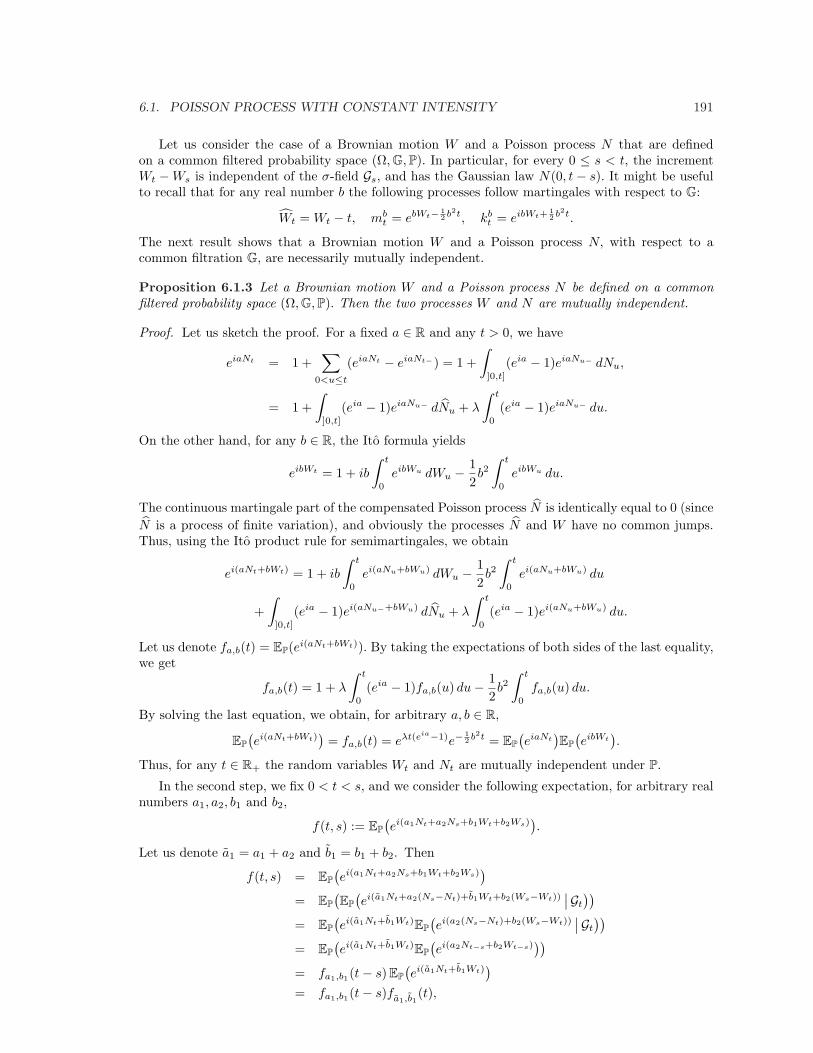
6.1. POISSON PROCESS WITH CONSTANT INTENSITY 191
Let us consider the case of a Brownian motion W and a Poisson process N that are definedon a common filtered probability space (Ω,G,P). In particular, for every 0 ≤ s < t, the incrementWt −Ws is independent of the σ-field Gs, and has the Gaussian law N(0, t− s). It might be usefulto recall that for any real number b the following processes follow martingales with respect to G:
Wt = Wt − t, mbt = ebWt− 1
2 b2t, kbt = eibWt+
12 b2t.
The next result shows that a Brownian motion W and a Poisson process N, with respect to acommon filtration G, are necessarily mutually independent.
Proposition 6.1.3 Let a Brownian motion W and a Poisson process N be defined on a commonfiltered probability space (Ω,G,P). Then the two processes W and N are mutually independent.
Proof. Let us sketch the proof. For a fixed a ∈ R and any t > 0, we have
eiaNt = 1 +∑
0<u≤t
(eiaNt − eiaNt−) = 1 +∫
]0,t]
(eia − 1)eiaNu− dNu,
= 1 +∫
]0,t]
(eia − 1)eiaNu− dNu + λ
∫ t
0
(eia − 1)eiaNu− du.
On the other hand, for any b ∈ R, the Ito formula yields
eibWt = 1 + ib
∫ t
0
eibWu dWu − 12b2
∫ t
0
eibWu du.
The continuous martingale part of the compensated Poisson process N is identically equal to 0 (sinceN is a process of finite variation), and obviously the processes N and W have no common jumps.Thus, using the Ito product rule for semimartingales, we obtain
ei(aNt+bWt) = 1 + ib
∫ t
0
ei(aNu+bWu) dWu − 12b2
∫ t
0
ei(aNu+bWu) du
+∫
]0,t]
(eia − 1)ei(aNu−+bWu) dNu + λ
∫ t
0
(eia − 1)ei(aNu+bWu) du.
Let us denote fa,b(t) = EP(ei(aNt+bWt)). By taking the expectations of both sides of the last equality,we get
fa,b(t) = 1 + λ
∫ t
0
(eia − 1)fa,b(u) du− 12b2
∫ t
0
fa,b(u) du.
By solving the last equation, we obtain, for arbitrary a, b ∈ R,
EP(ei(aNt+bWt)
)= fa,b(t) = eλt(eia−1)e−
12 b2t = EP
(eiaNt
)EP
(eibWt
).
Thus, for any t ∈ R+ the random variables Wt and Nt are mutually independent under P.
In the second step, we fix 0 < t < s, and we consider the following expectation, for arbitrary realnumbers a1, a2, b1 and b2,
f(t, s) := EP(ei(a1Nt+a2Ns+b1Wt+b2Ws)
).
Let us denote a1 = a1 + a2 and b1 = b1 + b2. Then
f(t, s) = EP(ei(a1Nt+a2Ns+b1Wt+b2Ws)
)
= EP(EP
(ei(a1Nt+a2(Ns−Nt)+b1Wt+b2(Ws−Wt))
∣∣Gt
))
= EP(ei(a1Nt+b1Wt)EP
(ei(a2(Ns−Nt)+b2(Ws−Wt))
∣∣Gt
))
= EP(ei(a1Nt+b1Wt)EP
(ei(a2Nt−s+b2Wt−s)
))
= fa1,b1(t− s)EP(ei(a1Nt+b1Wt)
)
= fa1,b1(t− s)fa1,b1(t),

192 CHAPTER 6. APPENDIX: CONDITIONAL POISSON PROCESS
where we have used, in particular, the independence of the increment Nt−Ns (and Wt−Ws) of theσ-field Gt, and the time-homogeneity of N and W. By setting b1 = b2 = 0 in the last formula, weobtain
EP(ei(a1Nt+a2Ns)
)= fa1,0(t− s)fa1,0(t),
while the choice of a1 = a2 = 0 yields
EP(ei(b1Wt+b2Ws)
)= f0,b1(t− s)f0,b1
(t).
It is not difficult to check that
fa1,b1(t− s)fa1,b1(t) = fa1,0(t− s)fa1,0(t)f0,b1(t− s)f0,b1
(t).
We conclude that for any 0 ≤ t < s and arbitrary a1, a2, b1, b2 ∈ R:
EP(ei(a1Nt+a2Ns+b1Wt+b2Ws)
)= EP
(ei(a1Nt+a2Ns)
)EP
(ei(b1Wt+b2Ws)
).
This means that the random variables (Nt, Ns) and (Wt,Ws) are mutually independent. By proceed-ing along the same lines, one may check that the random variables (Nt1 , . . . , Ntn) and (Wt1 , . . . , Wtn)are mutually independent for any n ∈ N and for any choice of 0 ≤ t1 < · · · < tn. ¤
Let us now examine the behavior of the Poisson process under a specific equivalent change ofthe underlying probability measure. For a fixed T > 0, we introduce a probability measure Q on(Ω,GT ) by setting
dQdP
∣∣∣GT
= ηT , P-a.s., (6.2)
where the Radon-Nikodym density process ηt, t ∈ [0, T ], satisfies
dηt = ηt−κ dNt, η0 = 1, (6.3)
for some constant κ > −1. Since Y := κN is a process of finite variation, (6.3) admits a uniquesolution, denoted as Et(Y ) or Et(κN); it can be seen as a special case of the Doleans (or stochastic)exponential. By solving (6.3) path-by-path, we obtain
ηt = Et(κN) = eYt
∏
0<u≤t
(1 + ∆Yu)e−∆Yu = eY ct
∏
0<u≤t
(1 + ∆Yu),
where Y ct := Yt −
∑0<u≤t ∆Yu is the path-by-path continuous part of Y. Direct calculations show
thatηt = e−κλt
∏
0<u≤t
(1 + κ∆Nu) = e−κλt(1 + κ)Nt = eNt ln(1+κ)−κλt,
where the last equality holds if κ > −1. Upon setting a = ln(1+ κ) in part (iii) of Proposition 6.1.2,we get Ma = η; this confirms that the process η follows a G-martingale under P. We have thusproved the following result.
Lemma 6.1.1 Assume that κ > −1. The unique solution η to the SDE (6.3) is an exponentialG-martingale under P. Specifically,
ηt = eNt ln(1+κ)−κλt = eNt ln(1+κ)−λt(κ−ln(1+κ)) = Mat , (6.4)
where a = ln(1+κ). In particular, the random variable ηT is strictly positive, Pa.s. and EP(ηT ) = 1.Furthermore, the process Ma solves the following SDE:
dMat = Ma
t−(ea − 1) dNt, Ma0 = 1. (6.5)
We are in a position to establish the well-known result, which states that under Q the processNt, t ∈ [0, T ], follows a Poisson process with the constant intensity λ∗ = (1 + κ)λ.

6.1. POISSON PROCESS WITH CONSTANT INTENSITY 193
Proposition 6.1.4 Assume that under P a process N is a Poisson process with intensity λ withrespect to the filtration G. Suppose that the probability measure Q is defined on (Ω,GT ) through (6.2)and (6.3) for some κ > −1.(i) The process Nt, t ∈ [0, T ], follows a Poisson process under Q with respect to G with the constantintensity λ∗ = (1 + κ)λ.(ii) The compensated process N∗
t , t ∈ [0, T ], defined as
N∗t = Nt − λ∗t = Nt − (1 + κ)λt = Nt − κλt,
follows a Q-martingale with respect to G.
Proof. From remark (iii) after Proposition 6.1.2, we know that it suffices to find λ∗ such that, forany fixed b ∈ R, the process M b, given as
M bt := ebNt−λ∗t(eb−1), ∀ t ∈ [0, T ], (6.6)
follows a G-martingale under Q. By standard arguments, the process M b is a Q-martingale if andonly if the product M bη is a martingale under the original probability measure P. But in view of(6.4), we have
M bt ηt = exp
(Nt
(b + ln(1 + κ)
)− t(κλ + λ∗(eb − 1)
)).
Let us write a = b + ln(1 + κ). Since b is an arbitrary real number, so is a. Then, by virtue of part(iii) in Proposition 6.1.2, we necessarily have
κλ + λ∗(eb − 1) = λ(ea − 1).
After simplifications, we conclude that, for any fixed real number b, the process M b defined by (6.6)is a G-martingale under Q if and only if λ∗ = (1 + κ)λ. In other words, the intensity λ∗ of N underQ satisfies λ∗ = (1 + κ)λ. Also the second statement is clear. ¤
Remark 6.1.2 Assume that G = FN , i.e., the filtration G is generated by some Poisson processN. Then any strictly positive G-martingale η under P is known to satisfy SDE (6.3) for some G-predictable process κ.
Assume that W is a Brownian motion and N follows a Poisson process under P with respect toG. Let η satisfy
dηt = ηt−(βt dWt + κ dNt
), η0 = 1, (6.7)
for some G-predictable stochastic process β and some constant κ > −1. A simple application of theIto’s product rule shows that if processes η1 and η2 satisfy:
dη1t = η1
t−βt dWt, dη2t = η2
t−κ dNt,
then the product ηt := η1t η2
t satisfies (6.7). Taking the uniqueness of solutions to the linear SDE(6.7) for granted, we conclude that the unique solution to this SDE is given by the expression:
ηt = exp( ∫ t
0
βu dWu − 12
∫ t
0
β2u du
)exp
(Nt ln(1 + κ)− κλt
). (6.8)
The proof of the next result is left to the reader as exercise.
Proposition 6.1.5 Let the probability Q be given by (6.2) and (6.8) for some constant κ > −1 anda G-predictable process β, such that EP(ηT ) = 1.
(i) The process W ∗t = Wt −
∫ t
0βu du, t ∈ [0, T ], follows a Brownian motion under Q, with respect to
the filtration G.(ii) The process Nt, t ∈ [0, T ], follows a Poisson process with the constant intensity λ∗ = (1 + κ)λunder Q, with respect to the filtration G.(iii) Processes W ∗ and N are mutually independent under Q.

194 CHAPTER 6. APPENDIX: CONDITIONAL POISSON PROCESS
6.2 Poisson Process with Deterministic Intensity
Let λ : R+ → R+ be any non-negative, locally integrable function such that∫∞0
λ(u) du = ∞. Bydefinition, the process N (with N0 = 0) is the Poisson process with intensity function λ if for every0 ≤ s < t the increment Nt − Ns is independent of the σ-field Gs, and has the Poisson law withparameter Λ(t)− Λ(s), where the hazard function Λ equals Λ(t) =
∫ t
0λ(u) du.
More generally, let Λ : R+ → R+ be a right-continuous, increasing function with Λ(0) = 0 andΛ(∞) = ∞. The Poisson process with the hazard function Λ satisfies, for every 0 ≤ s < t and everyk = 0, 1, . . .
PNt −Ns = k | Gs = PNt −Ns = k =(Λ(t)− Λ(s))k
k!e−(Λ(t)−Λ(s)).
Example 6.2.1 The most convenient and widely used method of constructing a Poisson processwith a hazard function Λ runs as follows: we take a Poisson process N with the constant intensityλ = 1, with respect to some filtration G, and we define the time-changed process Nt := NΛ(t). Theprocess N is easily seen to follow a Poisson process with the hazard function Λ, with respect to thetime-changed filtration G, where Gt = GΛ(t) for every t ∈ R+.
Since for arbitrary 0 ≤ s < t
EP(Nt −Ns | Gs) = EP(Nt −Ns) = Λ(t)− Λ(s),
it is clear that the compensated Poisson process Nt = Nt − Λ(t) follows a G-martingale under P. Asuitable generalization of Proposition 6.1.3 shows that a Poisson process with the hazard functionΛ and a Brownian motion with respect to G follow mutually independent processes under P. Theproof of the next lemma relies on a direct application of the Ito formula, and so it is omitted.
Lemma 6.2.1 Let Z be an arbitrary bounded, G-predictable process. Then the process MZ , givenby the formula
MZt = exp
(∫
]0,t]
Zu dNu −∫ t
0
(eZu − 1) dΛ(u)),
follows a G-martingale under P. Moreover, MZ is the unique solution to the SDE
dMZt = MZ
t−(eZt − 1) dNt, MZ0 = 1.
In case of a Poisson process with intensity function λ, it can be easily deduced from Lemma 6.2.1that, for any (Borel measurable) function κ : R+ → (−1,∞), the process
ζt = exp(∫
]0,t]
ln(1 + κ(u)) dNu −∫ t
0
κ(u)λ(u) du)
is the unique solution to the SDE
dζt = ζt−κ(t) dNt, η0 = 1.
Using similar arguments as in the case of constant κ, one can show that the unique solution to theSDE
dηt = ηt−(βt dWt + κ(t) dNt
), η0 = 1,
is given by the following expression:
ηt = ζt exp(∫ t
0
βu dWu − 12
∫ t
0
β2u du
). (6.9)
The next result generalizes Proposition 6.1.5. Again, the proof is left to the reader.

6.3. CONDITIONAL POISSON PROCESS 195
Proposition 6.2.1 Let Q be a probability measure equivalent to P on (Ω,GT ), such that the densityprocess η in (6.2) is given by (6.9). Then, under Q and with respect to G :(i) the process W ∗
t = Wt −∫ t
0βu du, t ∈ [0, T ], follows a Brownian motion,
(ii) the process Nt, t ∈ [0, T ], is a Poisson process with the intensity function λ∗(t) = 1 + κ(t)λ(t),(iii) processes W ∗ and N are mutually independent under Q.
6.3 Conditional Poisson Process
We start by assuming that we are given a filtered probability space (Ω,G,P) and a certain sub-filtration F of G. Let Φ be an F-adapted, right-continuous, increasing process, with Φ0 = 0 andΦ∞ = ∞. We refer to Φ as the hazard process. In some cases, we have Φt =
∫ t
0φu du for some
F-progressively measurable process φ with locally integrable sample paths. Then the process φ iscalled the intensity process. We are in a position to state the definition of the F-conditional Poissonprocess associated with Φ. Slightly different, but essentially equivalent, definition of a conditionalPoisson process (also known as the doubly stochastic Poisson process) can be found in Bremaud(1981) and Last and Brandt (1995).
Definition 6.3.1 A process N defined on a probability space (Ω,G,P) is called the F-conditionalPoisson process with respect to G, associated with the hazard process Φ, if for any 0 ≤ s < t andevery k = 0, 1, . . .
PNt −Ns = k | Gs ∨ F∞ =(Φt − Φs)k
k!e−(Φt−Φs), (6.10)
where F∞ = σ(Fu : u ∈ R+).
At the intuitive level, if a particular sample path Φ·(ω) of the hazard process is known, the processN has exactly the same properties as the Poisson process with respect to G with the (deterministic)hazard function Φ·(ω). In particular, it follows from (6.10) that
PNt −Ns = k | Gs ∨ F∞ = PNt −Ns = k | F∞,
i.e., conditionally on the σ-field F∞ the increment Nt −Ns is independent of the σ-field Gs.
Similarly, for any 0 ≤ s < t ≤ u and every k = 0, 1, . . . , we have
PNt −Ns = k | Gs ∨ Fu =(Φt − Φs)k
k!e−(Φt−Φs). (6.11)
In other words, conditionally on the σ-field Fu the process Nt, t ∈ [0, u], behaves like a Poissonprocess with the hazard function Φ. Finally, for any n ∈ N, any non-negative integers k1, . . . , kn,and arbitrary non-negative real numbers s1 < t1 ≤ s2 < t2 ≤ . . . ≤ sn < tn we have
P( n⋂
i=1
Nti −Nsi = ki)
= EP( n∏
i=1
(Φti − Φsi
)ki
ki!e−(Φti
−Φsi)).
Let us notice that in all conditional expectations above, the reference filtration F can be replacedby the filtration FΦ generated by the hazard process. In fact, an F-conditional Poisson process withrespect to G follows also a conditional Poisson process with respect to the filtrations: FN ∨ F andFN ∨ FΦ (with the same hazard process).
We shall henceforth postulate that EP(Φt) < ∞ for every t ∈ R+.
Lemma 6.3.1 The compensated process Nt = Nt − Φt follows a martingale with respect to G.

196 CHAPTER 6. APPENDIX: CONDITIONAL POISSON PROCESS
Proof. It is enough to notice that, for arbitrary 0 ≤ s < t,
EP(Nt − Φt | Gs) = EP(EP(Nt − Φt | Gs ∨ F∞) | Gs) = EP(Ns − Φs | Gs) = Ns − Φs,
where, in the second equality, we have used the property of a Poisson process with a deterministichazard function. ¤
Given the two filtrations F and G and the hazard process Φ, it is not obvious whether we may finda process N, which would satisfy Definition 6.3.1. To provide a simple construction of a conditionalPoisson process, we assume that the underlying probability space (Ω,G,P), endowed with a referencefiltration F, is sufficiently large to accommodate for the following stochastic processes: a Poissonprocess N with the constant intensity λ = 1 and an F-adapted hazard process Φ. In addition, wepostulate that the Poisson process N is independent of the filtration F
Remark 6.3.1 Given a filtered probability space (Ω,F,P), it is always possible to enlarge it in sucha way that there exists a Poisson process N with λ = 1, independent of the filtration F, and definedon the enlarged space.
Under the present assumptions, for every 0 ≤ s < t, any u ∈ R+, and any non-negative integerk, we have
PNt − Ns = k | F∞ = PNt − Ns = k | Fu = PNt − Ns = kand
PNt − Ns = k | F Ns ∨ Fs = PNt − Ns = k =
(t− s)k
k!e−(t−s).
The next result describes an explicit construction of a conditional Poisson process. This con-struction is based on a random time change associated with the increasing process Φ.
Proposition 6.3.1 Let N be a Poisson process with the constant intensity λ = 1, independent ofa reference filtration F, and let Φ be an F-adapted, right-continuous, increasing process. Then theprocess Nt = NΦt , t ∈ R+, follows the F-conditional Poisson process with the hazard process Φ withrespect to the filtration G = FN ∨ F.
Proof. Since Gs ∨ F∞ = FNs ∨ F∞, it suffices to check that
PNt −Ns = k | FNs ∨ F∞ =
(Φt − Φs)k
k!e−(Φt−Φs)
or, equivalently,
PNΦt − NΦs = k | F NΦs∨ F∞ =
(Φt − Φs)k
k!e−(Φt−Φs).
The last equality follows from the assumed independence of N and F. ¤
Remark 6.3.2 Within the setting of Proposition 6.3.1, any F-martingale is also a G-martingale, sothat Condition (M.1) is satisfied.
The total number of jumps of the conditional Poisson process is obviously unbounded withprobability 1. In some financial models, only the properties of the first jump are relevant, though.There exist many ways of constructing the conditional Poisson process, but Condition (F.1) is alwayssatisfied by the first jump of such a process, since it follows directly from Definition 6.3.1. In effect,if we denote τ = τ1, then for any t ∈ R+ and u ≥ t we have:
Pτ ≤ t | Fu = PNt ≥ 1 | Fu = PNt −N0 ≥ 1 | G0 ∨ Fu = Pτ ≤ u | F∞,where the last equality follows from (6.11). It is also clear, once more by (6.11), that Pτ ≤ t | Fu =e−Φu for every 0 ≤ t ≤ u.

6.3. CONDITIONAL POISSON PROCESS 197
Example 6.3.1 Cox process. In some applications, it is natural to consider a special case of anF-conditional Poisson process, with the filtration F generated by a certain stochastic process, repre-senting the state variables. To be more specific, on considers a conditional Poisson process with theintensity process φ given as φt = g(t, Yt), where Y is an Rd-valued stochastic process independentof the Poisson process N , and g : R+×Rd → R+ is a (continuous) function. The reference filtrationF is typically chosen to be the natural filtration of the process Y ; that is, we take F = FY . In sucha case, the resulting F-conditional Poisson process is referred to as the Cox process associated withthe state variables process Y, and the intensity function g.
Our last goal is to examine the behavior of an F-conditional Poisson process N under an equivalentchange of a probability measure. Let us assume, for the sake of simplicity, that the hazard process Φis continuous, and the reference filtration F is generated by a process W, which follows a Brownianmotion with respect to G. For a fixed T > 0, we define the probability measure Q on (Ω,GT ) bysetting:
dQdP
∣∣∣GT
= ηT , P-a.s., (6.12)
where the Radon-Nikodym density process ηt, t ∈ [0, T ], solves the SDE
dηt = ηt−(βt dWt + κt dNt
), η0 = 1, (6.13)
for some G-predictable processes β and κ such that κ > −1 and EP(ηT ) = 1. An application ofIto’s product rule shows that the unique solution to (6.13) is equal to the product νtζt, wheredνt = νtβt dWt and dζt = ζt−κt dNt, with ν0 = ζ0 = 1. The solutions to the last two equations are
νt = exp( ∫ t
0
βu dWu − 12
∫ t
0
β2u du
)
andζt = exp (Ut)
∏
0<u≤t
(1 + ∆Uu) exp (−∆Uu),
respectively, where we denote Ut =∫]0,t]
κu dNu. It is useful to observe that ζ admits the followingrepresentations:
ζt = exp(−
∫ t
0
κu dΦu
) ∏
0<u≤t
(1 + κu∆Nu),
and
ζt = exp( ∫
]0,t]
ln(1 + κu) dNu −∫ t
0
κu dΦu
).
Proposition 6.3.2 Let the Radon-Nikodym density of Q with respect to P be given by (6.12)–(6.13).Then the process W ∗
t = Wt−∫ t
0βu du, t ∈ [0, T ], follows a Brownian motion with respect to G under
Q, and the process
N∗t = Nt −
∫ t
0
κu dΦu = Nt −∫ t
0
(1 + κu) dΦu, ∀ t ∈ [0, T ], (6.14)
follows a G-martingale under Q. If, in addition, the process κ is F-adapted, then the process Nfollows under Q an F-conditional Poisson process with respect to G, and the hazard process of Nunder Q equals
Φ∗t =∫ t
0
(1 + κu) dΦu.

198 CHAPTER 6. APPENDIX: CONDITIONAL POISSON PROCESS

Bibliography
[1] S. Babbs and T.R. Bielecki. A note on short spreads. Working paper, 2003.
[2] T.R. Bielecki. A multivariate Markov model for simulating dependent migrations. Workingpaper.
[3] T.R. Bielecki, S. Crepey, M. Jeanblanc, and M. Rutkowski. Valuation of basket credit derivativesin the credit migrations environment. Working paper, 2005.
[4] T.R. Bielecki, M. Jeanblanc, and M. Rutkowski. Hedging of defaultable claims. In R.A. Car-mona, editor, Paris-Princeton Lecture on Mathematical Finance 2003, Lecture Notes in Math-ematics 1847, pages 1–132. Springer, 2004.
[5] T.R. Bielecki, M. Jeanblanc, and M. Rutkowski. Modelling and valuation of credit risk. InM. Frittelli and W. Runggaldier, editors, CIME-EMS Summer School on Stochastic Methods inFinance, Bressanone, Lecture Notes in Mathematics 1856, pages 27–126. Springer, 2004.
[6] T.R. Bielecki, M. Jeanblanc, and M. Rutkowski. PDE approach to valuation and hedging ofcredit derivatives. Quantitative Finance, 5:257–270, 2005.
[7] T.R. Bielecki, M. Jeanblanc, and M. Rutkowski. Completeness of a general semimartingalemarket under constrained trading. In M. do Rosario Grossinho, editor, Stochastic Finance,Lisbon, pages 83–106. Springer, 2006.
[8] T.R. Bielecki, M. Jeanblanc, and M. Rutkowski. Hedging of credit derivatives in models withtotally unexpected default. In J. Akahori, editor, Stochastic Processes and Applications toMathematical Finance, pages 35–100. World Scientific, 2006.
[9] T.R. Bielecki, M. Jeanblanc, and M. Rutkowski. Replication of contingent claims in a reduced-form credit risk model with discontinuous asset prices. Stochastic Models, 22:661–687, 2006.
[10] T.R. Bielecki, M. Jeanblanc, and M. Rutkowski. Hedging of basket credit derivatives in creditdefault swap market. Journal of Credit Risk, 3:91–132, 2007.
[11] T.R. Bielecki, M. Jeanblanc, and M. Rutkowski. Pricing and trading credit default swaps in ahazard process model. Working paper, 2007.
[12] T.R. Bielecki and M. Rutkowski. Credit Risk: Modelling, Valuation and Hedging. Springer,2002.
[13] T.R. Bielecki and M. Rutkowski. Dependent defaults and credit migrations. ApplicationesMathematicae, 30:121–145, 2003.
[14] T.R. Bielecki and M. Rutkowski. Modelling of the defaultable term structure: ConditionallyMarkov approach. IEEE Transactions on Automatic Control, 49:361–373, 2004.
[15] T.R. Bielecki, A. Vidozzi, and L. Vidozzi. Approach to valuation of credit basket products andratings triggered step-up bonds. Working paper, 2006.
199

200 BIBLIOGRAPHY
[16] F. Black and J.C. Cox. Valuing corporate securities: Some effects of bond indenture provisions.Journal of Finance, 31:351–367, 1976.
[17] F. Black and M. Scholes. The pricing of options and corporate liabilities. Journal of PoliticalEconomy, 81:637–654, 1973.
[18] C. Blanchet-Scalliet and M. Jeanblanc. Hazard rate for credit risk and hedging defaultablecontingent claims. Finance and Stochastics, 8:145–159, 2004.
[19] C. Bluhm, L. Overbeck, and C. Wagner. An Introduction to Credit Risk Modeling. Chapman& Hall, 2004.
[20] P. Bremaud. Point Processes and Queues. Martingale Dynamics. Springer, 1981.
[21] P. Bremaud and M. Yor. Changes of filtration and of probability measures. Z. Wahr. Verw.Gebiete, 45:269–295, 1978.
[22] M.J. Brennan and E.S. Schwartz. Convertible bonds: Valuation and optimal strategies for calland conversion. Journal of Finance, 32:1699–1715, 1977.
[23] M.J. Brennan and E.S. Schwartz. Analyzing convertible bonds. Journal of Financial andQuantitative Analysis, 15:907–929, 1980.
[24] D. Brigo. Constant maturity credit default pricing and market models. Working paper, 2004.
[25] E. Briys and F. de Varenne. Valuing risky fixed rate debt: An extension. Journal of Financialand Quantitative Analysis, 32:239–248, 1997.
[26] R. Bruyere. Les produits derives de credit. Economica, 2005.
[27] L. Campi and A. Sbuelz. Closed form pricing of benchmark equity default swaps under theCEV assumption. Working paper, 2005.
[28] P. Carr. Dynamic replication of a digital default claim. Working paper, 2005.
[29] N. Chen and S. Kou. Credit spreads, optimal capital structure, and implied volatility withendogenous default and jump risk. Working paper, 2005.
[30] U. Cherubini, E. Luciano, and W. Vecchiato. Copula Methods in Finance. J. Wiley, 2004.
[31] P.O. Christensen, C.R. Flor, D. Lando, and K.R. Miltersen. Dynamic capital structure withcallable debt and debt renegotiations. Working paper, 2002.
[32] P. Collin-Dufresne, R.S. Goldstein, and J.-N. Hugonnier. A general formula for valuing default-able securities. Econometrica, 72:1377–1407, 2004.
[33] D. Cossin and H. Pirotte. Advanced Credit Risk Analysis. J. Wiley, 2001.
[34] B. Dao. Approche structurelle du risque de credit avec des processus mixtes diffusion-sauts.PhD thesis, 2005.
[35] M. Davis and V. Lo. Infectious defaults. Quantitative Finance, 1:382–386, 2001.
[36] C. Dellacherie. Capacites et processus stochastiques. Springer, 1972.
[37] C. Dellacherie and P.A. Meyer. Probabilites et Potentiel, chapitres I-IV. Hermann, Paris, 1975.English translation: Probabilities and Potentiel, Chapters I-IV, North-Holland, 1978.
[38] C. Dellacherie and P.A. Meyer. A propos du travail de Yor sur les grossissements des tribus. InC. Dellacherie, P.A. Meyer, and M. Weil, editors, Seminaire de Probabilites XII, Lecture Notesin Mathematics 649, pages 69–78. Springer, 1978.

BIBLIOGRAPHY 201
[39] C. Dellacherie and P.A. Meyer. Probabilites et Potentiel, chapitres V-VIII. Hermann, Paris,1980. English translation: Probabilities and Potentiel, Chapters V-VIII, North-Holland, 1982.
[40] D. Duffie. First-to-default valuation. Working paper, 1998.
[41] D. Duffie and D. Lando. Term structure of credit spreads with incomplete accounting informa-tion. Econometrica, 69:633–664, 2000.
[42] D. Duffie, M. Schroder, and C. Skiadas. Recursive valuation of defaultable securities and thetiming of resolution of uncertainty. Annals of Applied Probability, 6:1075–1090, 1996.
[43] D. Duffie and K. Singleton. Simulating corellated defaults. Working paper, 1998.
[44] D. Duffie and K. Singleton. Credit Risk: Pricing, Measurement and Management. PrincetonUniversity Press, 2003.
[45] R. Elliott. Stochastic Calculus and Applications. Springer, 1982.
[46] R.J. Elliott, M. Jeanblanc, and M. Yor. On models of default risk. Mathematical Finance,10:179–196, 2000.
[47] Y. Elouerkhaoui. Etude des problemes de correlation et d’incompletude dans les marches decredit. PhD thesis, 2006.
[48] P. Embrechts, F. Lindskog, and A.J. McNeil. Modelling dependence with copulas and appli-cations to risk management. In S. Rachev, editor, Handbook of Heavy Tailed Distributions inFinance, pages 329–384. Elsevier Noth Holland, 2003.
[49] J-P. Florens and D. Fougere. Noncausality in continuous time. Econometrica, 64:1195–1212,1996.
[50] R. Frey, A.J. McNeil, and P. Embrechts. Risk Management. Princeton University Press, 2006.
[51] K. Giesecke. Default compensator, incomplete information, and the term structure of creditspreads. Working paper, 2002.
[52] Y.M. Greenfield. Hedging of the Credit Risk Embedded in Derivative Transactions. Phd thesis,2000.
[53] B. Hilberink and L.C.G. Rogers. Optimal capital structure and endogenous default. Financeand Stochastics, 6:237–263, 2002.
[54] J. Hull and A. White. Valuing credit default swaps (i): No counterparty default risk. Journalof Derivatives, 8:29–40, 2000.
[55] F. Jamshidian. Valuation of credit default swap and swaptions. Finance and Stochastics,8:343–371, 2004.
[56] R.A. Jarrow and F. Yu. Counterparty risk and the pricing of defaultable securities. Journal ofFinance, 56:1756–1799, 2001.
[57] M. Jeanblanc and Y. Le Cam. Intensity versus hazard process approach. Working paper, 2005.
[58] M. Jeanblanc and M. Rutkowski. Modeling default risk: An overview, pages 171–269. HighEducation Press. Beijing, 2000.
[59] M. Jeanblanc and M. Rutkowski. Modeling default risk: Mathematical tools. Working paper,2000.
[60] T. Jeulin and M. Yor. Nouveaux resultats sur le grossissement des tribus. Ann. Scient. ENS,4e serie, 11:429–443, 1978.

202 BIBLIOGRAPHY
[61] M. Kijima, K. Komoribayashi, and E. Suzuki. A multivariate Markov model for simulatingcorrelated defaults. Working paper, 2002.
[62] M. Kijima and Y. Muromashi. Credit events and the valuation of credit derivatives of baskettype. Review of Derivatives Research, 4:55–79, 2000.
[63] S. Kusuoka. A remark on default risk models. Advances in Mathematical Economics, 1:69–82,1999.
[64] D. Lando. On rating transition analysis and correlation. Risk Publications, 1998.
[65] D. Lando. Credit Risk Modeling. Princeton University Press, 2004.
[66] J.-P. Laurent and J. Gregory. Basket defaults swaps, CDOs and factor copulas. Working paper,2002.
[67] J.-P. Laurent and J. Gregory. Correlation and dependence in risk management. Working paper,2003.
[68] O. Le Courtois and F. Quittard-Pinon. The capital structure from the point of view of investorsand managers: An analysis with jump processes. Working paper, 2004.
[69] H. Leland. Corporate debt value, bond covenants, and optimal capital structure. Journal ofFinance, 49:1213–1252, 1994.
[70] H. Leland and K. Toft. Optimal capital structure, endogenous bankruptcy, and the termstructure of credit spreads. Journal of Finance, 51:987–1019, 1996.
[71] D.-X. Li. On default correlation: a copula approach. Journal on Fixed Income, 9:43–54, 1999.
[72] F.A. Longstaff and E.S. Schwartz. A simple approach to valuing risky fixed and floating ratedebt. Journal of Finance, 50:789–819, 1995.
[73] D. Madan and H. Unal. Pricing the risks of default. Review of Derivatives Research, 2:121–160,1998.
[74] R. Mansuy and M. Yor. Random Times and Enlargements of Filtrations in a Brownian Setting.Springer-Verlag, 2006.
[75] G. Mazziotto and J. Szpirglas. Modele general de filtrage non lineaire et equations differentiellesstochastiques associees. Ann. Inst. Henri Poincare, 15:147–173, 1979.
[76] A.J. McNeil, R. Frey, and P. Embrechts. Quantitative Risk Management: Concepts, Techniques,and Tools. Princeton University Press, Princeton, 2005.
[77] R. Merton. On the pricing of corporate debt: The risk structure of interest rates. Journal ofFinance, 3:449–470, 1974.
[78] F. Moraux. Valuing corporate liabilities when the default threshold is not an absorbing barrier.Working paper, 2002.
[79] T.N. Nielsen, J. Saa-Requejo, and P. Santa-Clara. Default risk and interest rate risk: The termstructure of default spreads. Working paper, 1993.
[80] A. Nikeghbali and M. Yor. A definition and some properties of pseudo-stopping times. Annalsof Probability, 33:1804–1824, 2005.
[81] M. Rutkowski and K. Yousiph. PDE approach to valuation and hedging of basket credit deriva-tives. International Journal of Theoretical and Applied Finance, 10:1261–1285, 2007.
[82] J. Saa-Requejo and P. Santa-Clara. Bond pricing with default risk. Working paper, 1999.

BIBLIOGRAPHY 203
[83] P. Schonbucher and D. Schubert. Copula-dependent default risk in intensity models. Workingpaper, 2001.
[84] P.J. Schonbucher. Credit Derivatives Pricing Models. Wiley Finance, 2003.
[85] D. Wong. A unifying credit model. Technical report, Capital Markets Group, 1998.
[86] C. Zhou. The term structure of credit spreads with jumps risk. Journal of Banking and Finance,25:2015–2040, 2001.