credit, asset prices, and financial stress
TRANSCRIPT

Credit, Asset Prices, and Financial Stress∗
Miroslav Misina and Greg TkaczBank of Canada
Historical narratives typically associate financial crises withcredit expansions and asset price misalignments. The questionis whether some combination of measures of credit and assetprices can be used to predict these events. Borio and Lowe(2002) answer this question in the affirmative for a sample ofthirty-four countries, but the question is surprisingly difficultto answer for individual developed countries that have facedvery few, if any, financial crises in the past. To circumvent thisproblem, we focus on financial stress and ask whether creditand asset price movements can help predict it. To measurefinancial stress, we use the financial stress index (FSI) devel-oped by Illing and Liu (2006). Other innovations include theestimation and forecasting using both linear and endogenousthreshold models, and a wide range of asset prices (stock andhousing prices, for example). The exercise is mainly performedfor Canada, but in our robustness checks we also consider datafor Japan and the United States. Our sample also includes thefinancial crisis of 2007–08.
JEL Codes: G10, E5.
1. Introduction
Despite the apparent uniqueness of each financial cycle—from theconditions that lead to boom times, to triggers that result inreversals—historical narratives (e.g., Kindleberger and Aliber 2005)
∗We would like to thank the participants and discussants at the Bank ofCanada, the “Forecasting Financial Markets” conference (Aix-en-Provence), the“Measuring and Forecasting Financial Stability” workshop (Dresden), the “Pro-vision and Pricing of Liquidity Insurance” conference (New York), AndrewLevin, and an anonymous referee for valuable comments and suggestions, aswell as Stephen Doxey and Thomas Carter for excellent research assistance.Author contact: Misina: [email protected]; Tel: 613-782-8271; Tkacz:[email protected]; Tel: 613-782-8591.
95

96 International Journal of Central Banking December 2009
suggest that most cycles display common features: boom times aretypically associated with periods of credit expansion and persistentincreases in asset prices, often followed by rapid reversals.
These commonalities, confirmed by recent empirical work (e.g.,Borio and Lowe 2002, Kaminsky and Reinhart 1999), suggest thatdevelopments in the credit and asset markets of individual countriesmay provide an early-warning indicator of vulnerability in the finan-cial system that would be useful in assessing the current situationand in discussions of possible policy actions. In light of this, it issomewhat surprising that the empirical work in this area is scarce(Borio and Lowe 2002, 11). Whatever reasons there may be at ageneral level, the problem in doing this type of analysis for devel-oped countries is compounded by the scarcity of events that wouldqualify as financial crises in those countries.1 Absence of financialcrises does not, however, mean that financial systems of developedcountries have not, or cannot, come under stress, but it does raisethe issue of the best way to proceed.
In this work we propose a methodology that can be used toassess the role of credit and asset prices as early-warning indica-tors of vulnerability in the financial system of countries that haveexperienced very few or no financial crises over the sample periodof interest. A typical example is Canada, which will be the basisof our empirical work in this paper: in Bordo et al. (2001) dating,Canada has not experienced any “twin crises” (banking and cur-rency crises) since the beginning of their sample in 1883, and hasexperienced only four currency crises since 1945.2 These features ofthe sample preclude a meaningful country-level analysis based onbinary indicators of crises. Instead, we suggest that in such circum-stances one focuses on incidences of financial stress. In our work weuse the financial stress index (FSI), a continuous measure of financialstress developed by Illing and Liu (2006). The measure was origi-nally developed for Canada, but the underlying approach can beapplied to any country. In our examination of the role of credit and
1Bordo et al. (2001, 55) define financial crises as episodes of financial mar-ket volatility marked by significant problems of illiquidity and insolvency amongfinancial market participants and/or by official intervention in order to containsuch consequences.
2For details and dating of crises, see the appendix to Bordo et al. (2001).

Vol. 5 No. 4 Credit, Asset Prices, and Financial Stress 97
asset price in episodes of financial stress we consider both linear andnonlinear models, since the latter may be more suitable in capturingany behavioral asymmetries of financial market participants.
It is important to emphasize that the objective of this type ofwork is not to forecast idiosyncratic events that cause reversals (animpossible task using any econometric model), but rather to assesswhether, historically, there has been a relationship between the var-ious measures of movements in credit and asset prices at time t andthe FSI k periods ahead. The working hypothesis is that movementsin credit and asset prices are indicators of the health of the systemand its ability to withstand various types of shocks. Since the impactof a shock depends not only on the state of the system but also onthe magnitude of the shock, one would expect that, everything elsebeing the same, excessive growth of credit and persistent increases inasset prices reduce the ability of the system to withstand the shocks.
To preview the main results, we find that within a linear frame-work, domestic credit growth is the best predictor of the FSI at allhorizons, resulting in marginally lower prediction errors relative toour base-case model, although we do not observe the combinationof credit and asset prices observed by Borio and Lowe (2002). Ourresults suggest that asset prices tend to be better predictors of stresswhen we allow for nonlinearities, suggesting that extreme asset pricemovements have disproportionate impact on financial stress. Finally,at the two-year horizon, business credit and real estate prices emergeas important predictors of financial stress, confirming the generalfindings of Borio and Lowe.
The presentation is organized as follows. In section 2 we reviewthe related literature and describe the nature of the problemaddressed in this paper. Section 3 discusses in detail the data used.In section 4, we describe the model and present our results. Section5 contains the results of our robustness checks, including the appli-cation of our approach to the United States and Japan. The lastsection concludes.
2. Related Literature
Broadly speaking, the present work forms part of the literatureattempting to arrive at a set of early-warning indicators. The general

98 International Journal of Central Banking December 2009
problem in this literature has been to identify a subset of macro-economic and other relevant variables that would help predict theprobability of a financial crisis.3
Borio and Lowe (2002) investigate the usefulness of asset pricesas indicators of financial crises. The authors establish some styl-ized facts regarding the behavior of asset prices over the last thirtyyears and conclude that there is a relationship between asset pricemovements, credit cycles, and developments in the real economy.Given this, they asked whether a useful indicator of financial crisescan be constructed. The exercise performed is to assess whethercredit, asset prices, and investments—either separately or in somecombination—can predict financial crises.4 The methodology used isthat of Kaminsky and Reinhart (1999), and it is based on thresholdvalues of each series. The dating of crises is taken from Bordo et al.(2001). The key finding is that some combination of asset prices andcredit gap can help predict crises.
Hanschel and Monnin (2005) focus on the banking sector andpropose an index that can be used to measure stress in the Swissbanking sector. The paper then investigates whether the values ofthe index can be predicted by a set of macro variables. In assessingthe latter, the authors follow Borio and Lowe (2002), focusing onthe imbalances rather than levels of variables.
This paper is related to Hanschel and Monnin’s work since itfocuses on a single country and investigates the predictive abilityof a set of variables for financial stress rather than as indicators of
3There have been a variety of papers that have explored a range of indicatorsfor different types of crises. Recent work has tended to cluster around specificfinancial crises. For example, following the Mexican Crisis in 1994, papers such asSachs, Tornell, and Velasco (1996) and Frankel and Rose (1996) explored whethera variety of variables—such as bank credit growth, currency reserves, capitalinflows, and level of the exchange rate—affect the likelihood of a crisis. Followingthe Asian crisis in 1997, there were more efforts, such as Goldstein and Hawkins(1998) and Rodrik and Velasco (1999). Berg and Pattillo (1998) test whether cri-sis prediction measures constructed after the Mexican crisis would have predictedthe Asian crisis. Sorge (2004) provides an excellent survey of stress-testing litera-ture and its relationship to macroeconomic forecasting and early-warning-signalsliterature.
4The idea that credit expansions may lead to imbalances and eventual crisesis certainly not new. Hayek (1932) is an early example in the twentieth century,but the views go further back. Schumpeter (1954) contains a historical survey ofthe key ideas by period, and their proponents.

Vol. 5 No. 4 Credit, Asset Prices, and Financial Stress 99
crises. In our work, however, the indicator of financial stress used isthe one developed by Illing and Liu (2006). This indicator is broaderbased than in Hanschel and Monnin, since it tries to capture stressin the financial system rather than only focusing on the bankingsector.
In exploring the forecasting ability of credit and asset prices forfinancial stress, we look at both linear and nonlinear (threshold)specifications. In the latter, we follow Borio and Lowe (2002) but,rather than specifying the threshold exogenously, in our work thethresholds are determined endogenously.
3. Data
3.1 A Measure of Financial Stress
Financial stress can be characterized as a situation in which largeparts of the financial sector face the prospects of large financiallosses. These situations are usually accompanied by an increaseddegree of perceived risk (a widening of the distribution of probablelosses) and uncertainty (decreased confidence in the shape of thatdistribution).
To capture these features of financial stress, Illing and Liu (2006)constructed a weighted average of various indicators of expected loss,risk, and uncertainty in the financial sector. The resulting financialstress index (FSI) is a continuous, broad-based measure that includesthe following indicators from equity, bond, and foreign exchangemarkets, as well as indicators of banking-sector performance:
• the spread between the yields on bonds issued by Canadianfinancial institutions and the yields on government bonds ofcomparable duration
• the spread between yields on Canadian nonfinancial corporatebonds and government bonds
• the inverted term spread (i.e., the ninety-day Treasury billrate minus the ten-year government yield)
• the beta derived from the total return index for Canadianfinancial institutions
• Canadian trade-weighted dollar GARCH volatility• Canadian stock market (TSX) GARCH volatility

100 International Journal of Central Banking December 2009
Figure 1. Financial Stress Index
• the difference between Canadian and U.S. government short-term borrowing rates
• the average bid-ask spread on Canadian Treasury bills• the spread between Canadian commercial paper rates and
Treasury bill rates of comparable duration
In constructing the FSI, Illing and Liu considered several weight-ing options and settled on weights that reflect relative shares ofcredit for particular sectors in the economy. The resulting index,shown in figure 1, was most effective in correctly signaling eventsthat are widely associated with high financial stress (e.g., the stockmarket crash in October 1987, the peso crisis in 1994, the long-term capital management crisis in 1998, etc.). This is not surprising,given that Canada is a small open economy whose markets are wellintegrated internationally. As such, it is not insulated from inter-national financial developments. Turmoil in international financialmarkets will be reflected in increased stress in Canadian markets.This does not mean that financial stress is not or cannot be domes-tically generated, but it may indicate that the level of “internal”stress is secondary to the level of “external” stress that spills over

Vol. 5 No. 4 Credit, Asset Prices, and Financial Stress 101
into Canadian financial markets. To assess the importance of exter-nal factors in predicting financial stress in Canada, we include a setof international explanatory variables described below.
3.2 Explanatory Variables
Because Canada is a small open economy, its financial stress willnecessarily be impacted by international events—the 1994 peso and1997 Asian crises being well-known recent examples. For this reason,our data set incorporates, in addition to a broad set of domestic vari-ables, several foreign variables. However, international developmentswill also be felt in many domestic variables. For example, Canadianstock prices move in response to expected future earnings of Cana-dian firms, which in turn are largely dependent on internationalfactors such as the economic health of Canada’s trading partnersor on world commodity prices. In addition, real estate prices followsimilar patterns across major international cities (e.g., see Shiller2005, 19). As a result, many of our variables will necessarily movein response to the ultimate source of the stress, be it domestic orinternational factors.
The explanatory variables are divided into four major cate-gories:5
(i) Credit measures: the growth rate of total householdcredit (HouseCR), total business credit (BusCR), and totalcredit/GDP (CR/Y)
(ii) Asset prices (growth rates): stock prices (TSX), commercialreal estate indices (real (ComREI) and nominal (real ComREI)), residential real estate indices (“New house price” andexisting (RoyalLePage)), average price to personal disposableincome ratio (AvgP/PDI), and Canadian dollar price of gold(GoldC$)
(iii) Macroeconomic variables: Investment/GDP (I/Y), GDPgrowth rate, money (M1++ and M2++), and inflation (TotalCPI and Core CPI)
5Unless otherwise indicated, the source of the data is the Bank of Canada.

102 International Journal of Central Banking December 2009
(iv) Foreign variables: crude oil, asset price indices (United States,Australia, Japan),6 world gold price, U.S. bank credit,7 U.S.federal funds rate, and world GDP
The data is quarterly and spans the period 1984–2006. The fore-casting exercise is performed over the period 1996–2006. The lastobservation is 2006:Q4. The explanatory variables are converted intogrowth rates, so all variables are stationary.8 We consider both quar-terly and annual growth rates, since it is possible that longer-runcumulative growth rates in the explanatory variables may containmore information about financial stress than quarterly growth rates.In our output we use d = 1 to denote quarterly growth rates andd = 4 for annual (year-over-year) growth rates.
4. Models and Results
4.1 Linear Models and Forecast Evaluation
In order to evaluate the marginal contributions of the variousexplanatory variables, we compare all our models with a simple lin-ear benchmark, whereby the current FSI is simply a function of thek-quarter lagged FSI:
FSIt = α + βFSIt−k + ε1,t. (1)
At this time, the explanatory variables will be added to (1) inisolation and in pairs; given the multitude of horizons and variablesunder consideration, this alone results in several thousand modelsto be assessed. The augmented models are thus
FSIt = α + β1FSIt−k + γXt−k + ε2,t, (2)
6These indices are the same ones used by Borio and Lowe (2002). In general,they are the aggregates of stock prices, bond prices, and real estate prices, butthe components vary by country depending on data availability. The reader isreferred to their paper for details.
7Source: Federal Reserve Board, H.8 Release: Assets and Liabilities of Com-mercial Banks in the United States. Available at http://www.federalreserve.gov/releases/h8/.
8Commercial real estate investment is not transformed, since it was found tobe stationary.

Vol. 5 No. 4 Credit, Asset Prices, and Financial Stress 103
where X is a vector containing one or two explanatory variables.Since we are primarily interested in forecast performance, we sum-marize the forecast performance according to the ratio of the rootmean squared error (RMSE) of model (2) relative to that of (1):
rmr =
√∑2006Q4t=1996Q1(FSI2,t − FSIt)2
/44√∑2006Q4
t=1996Q1(FSI1,t − FSIt)2/
44, (3)
where FSI1,t,FSI2,t are forecasts of the FSI originating from models(1) and (2), respectively. When the rmr is above 1.0, this indicatesthat the additional explanatory variables worsen the forecast per-formance relative to the base-case model; when it is below 1.0, theforecast performance is improved.9,10
To determine whether the ratio of mean-squared errors is sta-tistically less than 1.0, we employ a test proposed by McCracken(2004) that can test for equality of the mean-squared errors of nestedmodels. Let Dt+k denote the difference between the squared fore-cast errors at t + k of the base-case model (i.e., the model whichincludes only the lagged FSI) and the alternative model (i.e., themodel augmented with one or more explanatory variables):
Dt+k = ε21,t+k − ε2
2,t+k. (4)
With n forecast periods, the statistic for testing the equality ofmean-squared errors between the base-case and alternative model iscomputed as
9In comparisons of models that contain the same dependent variable, theabove is equivalent to a comparison of the adjusted R-squared of these mod-els. The adjustment factor for the R-squared imposes a penalty on the inclu-sion of additional explanatory variables. The adjusted R-squared of the resultingmodel will be lowered if the additional variable’s contribution does not exceedthe penalty factor. Consequently, the ratio of the adjusted R-squared statisticscould be greater than 1.
10This model selection criterion gives the same weight to the errors on theupside and the downside. To the extent that the users might give more weightto increases than decreases, a selection criterion that penalizes downside errorsmore than the upside ones would be more appropriate. We thank the referee forbringing this point to our attention.

104 International Journal of Central Banking December 2009
MSE − F = n∑ n−1 ∑T
t=R−k
(ε21,t+k − ε2
2,t+k
)n−1
∑Tt=R−k ε2
2,t+k
, (5)
where R represents the first out-of-sample forecast period (1996:Q1).Intuitively, note that the numerator represents the difference inmean-squared errors (MSEs) between the base-case and alternativemodel, and the denominator represents the MSE of the alternative.If both models produce equally accurate forecasts, then the numer-ator and test statistic are zero; if the base-case model has a lowerMSE, then the statistic will be negative, and it will be positive ifthe alternative model has a lower MSE. The distribution is nonstan-dard due to the fact that the models are nested, and so we use thecritical values computed by McCracken (2004). Results presented byMcCracken show that this test has good size and power for samplesizes as small as fifty. Our own application has a sample size of forty-four (1996:Q1 to 2006:Q4), so this test should be appropriate for ourpurposes. Instances where the alternative model is found to have astatistically lower MSE than the base-case model are highlighted inour figures.
The details of the forecasting exercise are as follows:
• We initially estimate (1) and (2) with data from 1984 to1996:Q1−k, where k = 1, 2, 4, 8, or 12.
• Using the estimated parameters, we produce a forecasted FSIfor 1996:Q1.
• We reestimate the parameters with data from 1984 to1996:Q2−k.
• We use the newly estimated parameters to obtain a forecastof the FSI for 1996:Q2.
• We continue in this fashion until forecasts have been generatedfor 2006:Q4, for a total of forty-four forecast periods.
Note that the above attempts to replicate actual real-time fore-casts, whereby the forecaster uses data available up to time t toproduce a forecast at t + k (or, equivalently, data up to t − k toproduce forecasts at time t). The issue of data revisions does notapply in the case of most of our financial variables, as these observa-tions are not revised. However, it is known that GDP and monetaryaggregates are subject to revision, so some caution should be used

Vol. 5 No. 4 Credit, Asset Prices, and Financial Stress 105
in interpreting some of these forecast results, as the data that weuse in these particular cases do not produce true real-time forecasts.
4.2 Threshold Specification
Equation (2) supposes that financial stress is a linear function ofasset price movements and other variables. However, if one believesthat unusually large movements in asset prices, credit, monetaryexpansion, etc., may lead to greater financial uncertainty if, forexample, herding mentality replaces rational financial decisions, thenthe relationship between some of our explanatory variables and theFSI may be nonlinear.11 We can approximate such relationships byallowing for threshold effects between the explanatory variables andthe FSI, such that the parameters of the models are allowed to dif-fer when the explanatory variables lie above or below their thresholdvalues. A similar strategy was employed by Borio and Lowe (2002),but the thresholds used in that study were explicitly specified bythe authors. We employ a more general approach, whereby we esti-mate the threshold values; these endogenous thresholds thereforemaximize the probability of locating a threshold effect in the data.
The threshold models take the form
FSIt = α1 + β1FSIt−k + γ1Xt−k + δ1zt−k + ξt for zk,t−k ≤ τ(6)
FSIt = α2 + β2FSIt−k + γ2Xt−k + δ2zt−k + ξt for zk,t−k > τ,(7)
where z is some variable extracted from the vector X, and τ rep-resents the level of z that triggers a regime change. We allow fora threshold effect for each of our twenty-four explanatory variables.Superscripts denote the values taken in regimes 1 and 2, respectively.
To estimate the parameters of the threshold model (6)–(7), wefollow Hansen (2000) who derives an approximation of the asymp-totic distribution of the least-squares estimator of the thresholdparameter τ . To understand how the parameters are estimated, we
11Regardless of the underlying mechanism, Misina and Tessier (2008) showthat nonlinearities play the key role in capturing extreme events associated withstress, as well as in generating plausible responses to shocks.

106 International Journal of Central Banking December 2009
introduce an indicator function w and can rewrite equations (6) and(7) as a single equation:
FSI t = α2 + β2FSI t−k + γ2Xt−k + δ2zt−k + Aw
+ BwFSI t−k + CwXt−k + Dwzt−k + ξt, (8)
where
w ={
1 zt−k ≤ τ0 zt−k > τ
,
α2 + A = α1, β2 + B = β1, γ2 + C = γ1, and δ2 + D = δ1.
By assuming that τ is bounded by the largest and smallest valuesof the threshold variables, we can estimate the parameters in (8) byleast squares conditional on a given value of τ . By iterating throughthe possible values of τ in the range of available threshold values,we select the τ that minimizes the sum of squared residuals in (8).
The forecast exercise using the threshold models proceeds inexactly the same manner as for the linear models described above,so the parameters and threshold values are reestimated each period.The rmr is computed as the ratio of the RMSE from (8) relative tothe RMSE of a modified version of the simple base-case model (1)which allows for threshold effects in the lagged value of the FSI.
4.3 Results
Given all the combinations of variables, horizons, and specifications,we consider 11,520 models relative to the base-case model (1).12 Tosummarize these results in the least cumbersome manner, we presentthe ratio of root mean squared errors for each horizon (k) and differ-encing operator (d) and model specification (linear or threshold) intwenty different graphs. This provides a simple visual approach tojudge the usefulness of various variables. Since the results for d = 1and d = 4 are very similar, we place the latter in an appendix.
The forecast performance of the linear models is summarized infigure 2. To interpret these figures, consider panel A. The horizontalaxis contains labels for all the explanatory variables considered
12This is based on 24×24 variable combinations, five horizons, two differencingoperators, and two model specifications: 576 × 5 × 2 × 2 = 11,520.

Vol. 5 No. 4 Credit, Asset Prices, and Financial Stress 107
Figure 2. Linear Models, Forecast Performance, d = 1
(twenty-four variables). When a variable is listed along the hori-zontal axis, this indicates that it is included as the first regressor inthe next twenty-four models. After each label there are twenty-fourbars, corresponding to the rmr’s associated with models using dif-ferent combinations of the labeled explanatory variable with othervariables. For example, the first variable on the horizontal axis is thecredit-to-GDP ratio, CR/Y. The first bar is the rmr for a model thatincludes only the CR/Y ratio as an additional explanatory variable,so that the estimated model is
FSI t = α + β1FSI t−k + γ1(CR/Y )t−k + εt.

108 International Journal of Central Banking December 2009
The second bar is the rmr for a model including the CR/Y aswell as the investment-to-GDP (I/Y) variable:
FSIt = α + β1FSIt−k + γ1(CR/Y )t−k + γ2(I/Y )t−k + εt.
The third bar is the rmr for the model
FSIt = α + β1FSIt−k + γ1(CR/Y )t−k + γ2(ComREI)t−k + εt,
etc.The results associated with different models are assessed against
the benchmark value of rmr = 1, which indicates that the inclusionof additional explanatory variables did not impact the forecastingperformance of the base-case model. As stated earlier, rmr > 1indicates that the inclusion of the variable has resulted in deterio-ration of the forecasting performance of the model relative to thebenchmark. Finally, rmr < 1 indicates improved performance of thenew model relative to the benchmark. Models for which the rmr isstatistically lower than 1.0 according to the McCracken (2004) testare denoted in white.
Returning to figure 2, it is clear that the only variable that con-sistently helps forecast the FSI is domestic business credit, althoughthe federal funds rate is significant at shorter horizons (up to twoquarters ahead). For both these variables we find that, regardlessof which variable they are paired with, they often produce mean-squared errors that are statistically lower than 1.0.
To understand the effect of business credit on the FSI, we cananalyze the estimated parameters of the best forecasting modelsat each horizon, which are presented in table 1. We note severalinteresting results. First, the explanatory power of the lagged FSIdecreases as the forecast horizon k increases, as evidenced by theadjusted R2 which steadily decreases from 0.58 for k = 1 to 0.00for k = 12. Second, the federal funds rate is retained in the bestforecasting models at the shorter horizons (k = 1, 2), while domes-tic credit is retained at all horizons. Third, the parameters on thecredit variables are all positive and statistically significant. This sig-nals that a 1 percent quarterly increase in credit will cause the FSIto increase by between one and two points in the following quar-ters, which signals higher stress. If business credit is expanding, thiscould indicate that financial institutions are adding more risk to

Vol. 5 No. 4 Credit, Asset Prices, and Financial Stress 109
Tab
le1.
In-S
ample
Reg
ress
ion
Res
ults,
Lin
ear
Model
s,B
ase-
Cas
ean
dB
est
For
ecas
ting
Model
s,d
=1
Sam
ple
:19
84:Q
1to
2006
:Q4
Var
iable
k=
1k
=2
k=
4k
=8
k=
12C
onst
ant
7.66
11.2
514
.31
21.2
119
.40
28.4
630
.43
40.0
145
.80
52.1
9(2
.27)
(3.5
6)(3
.77)
(5.4
7)(5
.62)
(7.0
4)(6
.32)
(7.8
0)(8
.27)
(10.
48)
FSI
t−k
0.75
0.76
0.54
0.54
0.30
0.39
0.04
0.15
−0.
19−
0.11
(12.
29)
(11.
42)
(7.2
3)(6
.53)
(4.3
1)(4
.43)
(0.3
9)(1
.49)
(−2.
09)
(−1.
07)
Bus
ines
s0.
68—
1.13
—2.
13—
1.34
—1.
59—
Cre
dit t
−k
(2.5
4)(3
.32)
(7.4
7)(4
.08)
(4.6
4)
Wor
ldG
DP
t−k
——
−0.
01—
——
——
——
(−1.
89)
Japa
nA
PI t
−k
——
——
——
——
0.36
—(2
.76)
Cor
eC
PI t
−k
——
——
——
2.29
——
—(3
.11)
Fed
Fund
s t−
k2.
07—
1.58
—−
2.32
——
——
—(1
.99)
(5.4
7)(−
1.11
)
R2
0.62
0.58
0.41
0.29
0.44
0.14
0.29
0.01
0.35
0.00
RM
SERat
io0.
920.
890.
780.
870.
82
Note
:T
heba
se-c
ase
mod
elin
clud
eson
lyth
ela
gged
FSI
.R
MSE
Rat
iois
the
rati
oof
root
mea
nsq
uare
der
ror
ofth
em
odel
con-
tain
ing
exog
enou
sre
gres
sors
rela
tive
toth
eba
se-c
ase
mod
el.
t-st
atis
tics
corr
ecte
dfo
rse
rial
corr
elat
ion
and
hete
rosk
edas
tici
tyar
ein
pare
nthe
ses.

110 International Journal of Central Banking December 2009
Figure 3. Threshold Models, Forecast Performance, d = 1
their balance sheets, and so results in a rise in the FSI. Conversely,when business credit falls, the opposite occurs. At shorter horizons,the federal funds rate is positively correlated with financial stress inCanada. That result is reversed at the one-year horizon, althoughthe parameter is not statistically significant.
The results for threshold models are presented in figure 3, andthe estimated coefficients for the best specifications are presented intable 2. The interpretation of these figures is similar to the linearmodel, except that in each model a threshold effect is allowed in thevariable labeled in the figure. For example, the first variable on thehorizontal axis in figure 3 is CR/Y, and the first bar is the rmr forthe model that includes only the CR/Y ratio, with threshold effect,as an additional explanatory variable. The second bar is the rmr for
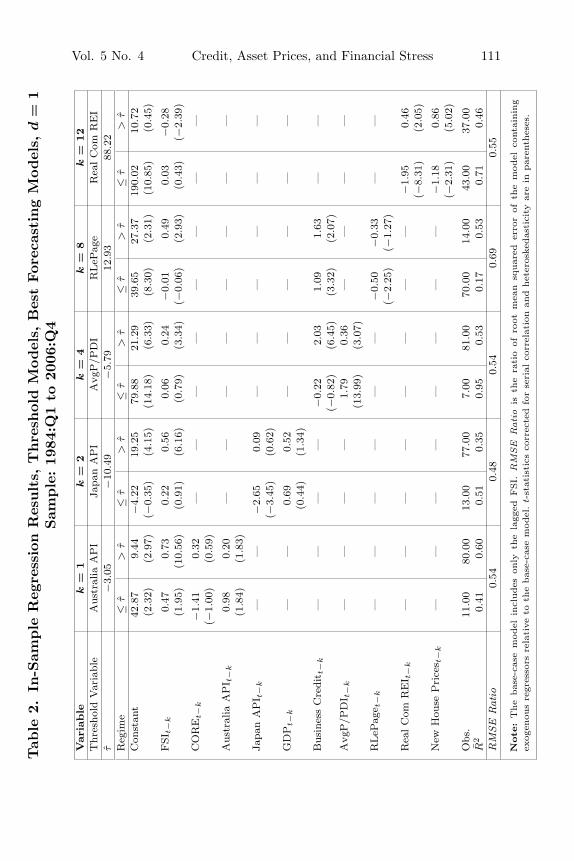
Vol. 5 No. 4 Credit, Asset Prices, and Financial Stress 111
Tab
le2.
In-S
ample
Reg
ress
ion
Res
ults,
Thre
shol
dM
odel
s,B
est
For
ecas
ting
Model
s,d
=1
Sam
ple
:19
84:Q
1to
2006
:Q4
Var
iable
k=
1k
=2
k=
4k
=8
k=
12
Thr
esho
ldV
aria
ble
Aus
tral
iaA
PI
Japa
nA
PI
Avg
P/P
DI
RLeP
age
Rea
lC
omR
EI
τ−
3.05
−10
.49
−5.
7912
.93
88.2
2R
egim
e≤
τ>
τ≤
τ>
τ≤
τ>
τ≤
τ>
τ≤
τ>
τ
Con
stan
t42
.87
9.44
−4.
2219
.25
79.8
821
.29
39.6
527
.37
190.
0210
.72
(2.3
2)(2
.97)
(−0.
35)
(4.1
5)(1
4.18
)(6
.33)
(8.3
0)(2
.31)
(10.
85)
(0.4
5)
FSI
t−k
0.47
0.73
0.22
0.56
0.06
0.24
−0.
010.
490.
03−
0.28
(1.9
5)(1
0.56
)(0
.91)
(6.1
6)(0
.79)
(3.3
4)(−
0.06
)(2
.93)
(0.4
3)(−
2.39
)
CO
RE
t−k
−1.
410.
32—
——
——
——
—(−
1.00
)(0
.59)
Aus
tral
iaA
PI t
−k
0.98
0.20
——
——
——
——
(1.8
4)(1
.83)
Japa
nA
PI t
−k
——
−2.
650.
09—
——
——
—(−
3.45
)(0
.62)
GD
Pt−
k—
—0.
690.
52—
——
——
—(0
.44)
(1.3
4)
Bus
ines
sC
redi
t t−
k—
——
—−
0.22
2.03
1.09
1.63
——
(−0.
82)
(6.4
5)(3
.32)
(2.0
7)A
vgP
/PD
I t−
k—
——
—1.
790.
36—
——
—(1
3.99
)(3
.07)
RLeP
age t
−k
——
——
——
−0.
50−
0.33
——
(−2.
25)
(−1.
27)
Rea
lC
omR
EI t
−k
——
——
——
——
−1.
950.
46(−
8.31
)(2
.05)
New
Hou
seP
rice
s t−
k—
——
——
——
—−
1.18
0.86
(−2.
31)
(5.0
2)
Obs
.11
.00
80.0
013
.00
77.0
07.
0081
.00
70.0
014
.00
43.0
037
.00
R2
0.41
0.60
0.51
0.35
0.95
0.53
0.17
0.53
0.71
0.46
RM
SERat
io0.
540.
480.
540.
690.
55
Note
:T
he
bas
e-ca
sem
odel
incl
udes
only
the
lagg
edFSI.
RM
SE
Rat
iois
the
rati
oof
root
mea
nsq
uar
eder
ror
ofth
em
odel
cont
ainin
gex
ogen
ous
regr
esso
rsre
lati
veto
the
bas
e-ca
sem
odel
.t-
stat
isti
csco
rrec
ted
for
seri
alco
rrel
atio
nan
dhet
eros
kedas
tici
tyar
ein
par
enth
eses
.

112 International Journal of Central Banking December 2009
the model that allows for the threshold effect in CR/Y and includesI/Y as an additional explanatory variable, etc.
The key features of the results at given horizon k, are as follows:
• k = 1, 2: No single variable appears to universally performwell at forecasting the FSI at very short horizons, as evidencedby the large number of black bars in one-quarter-ahead fore-casting models. The situation improves noticeably two quar-ters ahead, but in both cases, the forecast performance variesaccording to the specific combinations of variables that areretained, as well as the choice of the threshold variable. Thebest forecasting equations at these horizons retain core infla-tion and GDP, with international asset price indices (Aus-tralia, Japan) identified as threshold variables (table 2). Thermr at these horizons is quite low, indicating a significantimprovement in forecast performance relative to the base-casemodel.
• k = 4, 8: At these horizons, both business credit andasset prices emerge as significant predictors of financial stress(table 2). In both cases, a variable related to housing pricesappears as a significant threshold variable. The rmr in bothspecifications remains quite low, indicating improvements inthe forecast performance. For k = 8, the equation shows thatwhen house prices rise by more than 13 percent during a quar-ter, the impact of additional business credit on the FSI risesfrom 1.1 to 1.6, so business credit expansion during a housingboom can add additional financial stress two years later.
• k = 12: At the longer horizons, we observe that few vari-ables retain any forecasting power, the notable exception beingthe commercial real estate variable. At this horizon, commer-cial real estate investment is the regime-change trigger, whilenew house prices is retained as a significant regressor. Regimeeffects are quite pronounced for this equation, as the signs onboth parameters actually change depending on which regimewe are in. Furthermore, the number of observations in eachregime are almost equal. When commercial real estate invest-ment is low, increases in this variable and in new house priceslower stress; when commercial real estate investment is high,increases in these variables increase stress.

Vol. 5 No. 4 Credit, Asset Prices, and Financial Stress 113
Figure 4. Actual and Fitted FSI
Finally, to provide a sense of how these models track the actualdata, we plot in figure 4 the actual and fitted values of the bestlinear and threshold forecasting models for k = 4, a horizon whichcould be of interest to policymakers. In both cases, business credit is

114 International Journal of Central Banking December 2009
retained as a regressor and we see that, in general, both models per-form reasonably well in tracking the trend and turning points of theFSI. The improvement of the threshold model relative to the linearmodel centers on the seven observations early in the sample, wherethe threshold model succeeds in picking up a few extreme move-ments of the FSI. One would therefore conclude that at this horizonbusiness credit offers some hope in forecasting the FSI, regardless ofthe specification used.
5. Robustness Checks
To verify whether credit and asset prices are useful predictors offinancial stress more generally, we first assess whether some of themore promising variables are good predictors of stress in Japan andthe United States; second, we consider how these variables movedprior to the 2007–08 financial crisis.
5.1 The Crisis of 2007–08
In August 2007, the FSI increased sharply, pointing to consider-able stress in the Canadian financial system. Indeed, the FSI in therecent episode reached its historical high, indicating that this is themost stressful episode since 1985. To assess the predictive powerof the best forecasting model identified in the previous section, wehave extended the sample to 2008:Q2 and performed a forecast-ing exercise along the lines described in the previous section. Theresults are shown in figure 5. The results show that whereas thebest forecasting model does generate an increase in the FSI, themagnitude of that increase underestimates the increase in the FSIby a large margin. This is not surprising, given that the increasein stress captured by the FSI was largely triggered by exogenousevents (collapse of the U.S. subprime market), but an analysis ofthe behavior of the explanatory variables can provide additionalinsights.
A look at the two key explanatory variables retained in the bestthreshold specification (figure 6) reveals that while both variablespeaked in 2007:Q2, neither was anywhere near their historical highs.This may be an important contributing factor to the relatively good

Vol. 5 No. 4 Credit, Asset Prices, and Financial Stress 115
Figure 5. 2007–08 Crisis
Figure 6. Behavior of the Explanatory Variables

116 International Journal of Central Banking December 2009
health of the Canadian system and its resilience to date. Of course,the impact of a shock on the system is a function of the magnitudeof the shock as well, and the peak in the FSI in spite of the goodhealth of the system indicates that this is a large shock, by historicalstandards.
5.2 Results for Japan and the United States
We begin by constructing financial stress indexes for Japan andthe United States that are as comparable as possible to the onewe use for Canada.13 We choose these two countries since theirfinancial systems are quite different and have experienced differentshocks over the last several years, so the degree of predictability offinancial stress by credit and asset prices for these two countriescan be informative with regard to their robustness as indicators.We notice in figures 7 and 8 that the movements in the U.S. FSIare generally similar to that of Canada’s, with notable peaks in2001 and 2008, while the Japan FSI experienced more independentmovements.
To assess the usefulness of credit and asset prices in predictingthe FSIs in these countries, we focus solely on the case of d = 1 andk = 8 (the eight-quarter forecast horizon). In this context, we foundfor Canada that the lowest forecast errors could be obtained usinghousing prices and business credit, with the former serving as thethreshold variable. The Japan and U.S. variables that most closelymatched the Canadian definitions of these variables are residentialland prices14 (from the Japanese Real Estate Institute) and totalprivate-sector credit (from the International Monetary Fund) forJapan, and housing prices (Case-Shiller composite ten-city index)and total business credit (from the Federal Reserve bank of St.Louis’s FRED database) for the United States. The threshold vari-able is land/housing prices. The out-of-sample forecasted values forthe period 1998 to 2008 are presented in figures 7 and 8, allowing
13Details about the FSIs for Japan and the United States are available fromthe authors upon request.
14Land prices are the key driver of housing prices in Japan, so this is why weuse this variable to capture real estate prices in Japan.

Vol. 5 No. 4 Credit, Asset Prices, and Financial Stress 117
Figure 7. Forecasting the FSI for Japan
Figure 8. Forecasting the FSI for the United States

118 International Journal of Central Banking December 2009
us to assess whether such variables could have predicted the recentspike in the U.S. FSI.
For Japan, although its FSI is somewhat more volatile than thatof the United States and Canada, land prices and credit growthpredicted some peaks and troughs relatively well; for example, thecycle from early 2002 to mid-2004 was captured quite accuratelyeight quarters in advance. Other episodes, such as the financial stressspike in 2006, were not captured by these variables. This suggeststhat financial stress was being driven by other factors in this period,so forecasters should consider additional predictors of financial stressfor Japan.15
In the United States (figure 8) we observe that the forecastedvalues generally captured the level and volatility of actual FSI untilabout 2003, but from 2004 to 2007 it overpredicted stress, and itunderpredicted stress in 2008. Most recently, housing and creditgrowth predicted a sharp increase in stress in late 2007, whichmaterialized, but the subsequent stress actually overshot the pre-dicted values. Given that housing prices are known to have increaseddramatically until 2007 and then suffered a serious correction, theextent of the bubble characteristics of the U.S. housing market wasonly partially captured by the simple threshold relationship that weconsider.
In short, credit growth and housing prices appear to predict thedirection of the FSI relatively well eight quarters in advance. Thechallenge appears to obtain better predictions of the level of stress.To this end, although the threshold model that we use can capturesome of the “bubble” features of asset prices, in future work onemay wish to consider models with richer nonlinear dynamics. In themost recent episode, housing prices experienced a long and sustainedbuildup and then suffered a dramatic crash. Since our model over-predicted stress during the buildup phase, forecasters may wish tofocus their attention on building models that more adequately cap-ture the dynamics between asset prices and financial stress in suchperiods.
15Our last observation for the Japan FSI is 2007:Q3, so it predates the mostrecent global financial crisis.

Vol. 5 No. 4 Credit, Asset Prices, and Financial Stress 119
6. Conclusion
The literature on financial stress typically equates financial stresswith the occurrence of financial crises, and attempts to forecast thelatter using different sets of macroeconomic variables. This proce-dure runs into difficulties when applied to countries where financialcrises are rare or non-existent events, and this is evident especiallywhen the analysis is constrained by data availability to the lasttwenty-five to thirty years. The absence of financial crises, however,does not imply that a country has not been subjected to financialstress in the past, or that accumulated financial imbalances couldnot result in financial crises in the future.
To deal with the problem of measurement of financial stress inthe absence of financial crises, Illing and Liu (2006) constructeda financial stress index for Canada. The question we asked in thispaper is whether a set of explanatory variables commonly consideredin the macroprudential literature could help forecast financial stress.To do this we have considered both linear and threshold models andassessed their performance by comparing them with the benchmarkmodel in which the future value of the FSI is predicted using onlyits lagged value.
We find that, in line with the macroprudential literature, somecombination of credit and asset price variables are important pre-dictors of financial stress, although the results depend on the typeof model used (linear or threshold) and the forecast horizon. As ageneral rule, we find that these indicators offer greater value addedat forecasting the FSI than the benchmark model as the forecasthorizon increases. A specific indicator worthy of being highlightedis business credit, which emerges as the prominent leading indi-cator in both linear and nonlinear models at the one- and two-year horizons. A combination of this variable with a threshold ina housing-sector asset price leads to significant improvements inperformance over the same horizon. At shorter horizons, the fed-eral funds rate emerges as a predictor of financial stress in linearmodels. In general, however, international variables seem to playa smaller role than one would expect they would in a small openeconomy.
At the one-year horizon, which could be of interest to forward-looking policymakers, in practical terms there is little to distinguish

120 International Journal of Central Banking December 2009
the linear and threshold specifications, as both models track the FSIrelatively well at this horizon. What matters most is the monitoringof business credit, which emerges as an important leading indicatoramong all variables considered in our study.
The empirical results reported here are country specific, anda more in-depth comparative study of determinants of financialstress in countries with few or no financial crises would be instruc-tive. The methodology proposed in our work is well suited for thattask.
Appendix
Figure 9. Linear Models, Forecast Performance, d = 4

Vol. 5 No. 4 Credit, Asset Prices, and Financial Stress 121
Figure 10. Threshold Models, Forecast Performance,d = 4
References
Berg, A., and C. A. Pattillo. 1998. “Are Currency Crises Pre-dictable? A Test.” IMF Working Paper No. 98/154.
Bordo, M., B. Eichengreen, D. Klingebiel, and M. S. Martinez-Peria.2001. “Is the Crisis Problem Growing More Severe?” EconomicPolicy 16 (32): 51–82.
Borio, C., and P. Lowe. 2002. “Asset Prices, Financial and Mon-etary Stability: Exploring the Nexus.” BIS Working Paper No.114 (July).
Frankel, J. A., and A. K. Rose. 1996. “Currency Crashes in Emerg-ing Markets: An Empirical Treatment.” Journal of InternationalEconomics 41 (3–4): 351–66.

122 International Journal of Central Banking December 2009
Goldstein, M., and J. Hawkins. 1998. “The Origin of the AsianFinancial Turmoil.” Reserve Bank of Australia Research Discus-sion Paper No. 980 (May).
Hanschel, E., and P. Monnin. 2005. “Measuring and ForecastingStress in the Banking Sector: Evidence from Switzerland.” InBIS Papers No. 22: Investigating the Relationship Between theFinancial and Real Economy, 431–49. Bank for InternationalSettlements.
Hansen, B. E. 2000. “Sample Splitting and Threshold Estimation.”Econometrica 68 (3): 575–603.
Hayek, F. A. 1932. “Monetary Theory and the Trade Cycle.” InPrices & Production and Other Works (2008), ed. J. T. Salerno.Ludwig von Mises Institute.
Illing, M., and Y. Liu. 2006. “Measuring Financial Stress in a Devel-oped Country: An Application to Canada.” Journal of FinancialStability 2 (3): 243–65.
Kaminsky, G. L., and C. M. Reinhart. 1999. “The Twin Crises: TheCauses of Banking and Balance-of-Payments Problems.” Amer-ican Economic Review 89 (3): 473–500.
Kindleberger, C. P., and R. Aliber. 2005. Manias, Panics, andCrashes: A History of Financial Crises. 5th ed. John Wiley &Sons.
McCracken, M. W. 2004. “Asymptotics for Out-of-Sample Tests ofGranger Causality.” Working Paper, University of Missouri.
Misina, M., and D. Tessier. 2008. “Non-linearities, Model Uncer-tainty, and Macro Stress Testing.” Bank of Canada WorkingPaper No. 2008–30.
Rodrik, D., and A. Velasco. 1999. “Short-Term Capital Flows.”NBER Working Paper No. 7364.
Sachs, J. D., A. Tornell, and A. Velasco. 1996. “Financial Crisesin Emerging Markets: The Lessons from 1995.” In BrookingsPapers on Economic Activity, 1:1996, ed. W. C. Brainard andG. L. Perry, 147–215. Washington, DC: Brookings Institution.
Schumpeter, J. A. 1954. History of Economic Analysis. OxfordUniversity Press.
Shiller, R. J. 2005. Irrational Exuberance. 2nd ed. New York: Dou-bleday.
Sorge, M. 2004. “Stress-Testing Financial Systems: An Overviewof Current Methodologies.” BIS Working Paper No. 165(December).