Creativity Under Fire:

The Effects of Competition on Creative Production

Daniel P. Gross∗

NBER and Harvard Business School

August 1, 2015

Abstract:

Though fundamental to innovation and essential to numerous occupations and industries, the creative acthas received limited attention in economics and has historically proven difficult to study. This paper studiesthe incentive effects of competition on individuals’ creative production. Using a sample of commerciallogo design competitions, and a novel, content-based measure of originality, I find that competition has aninverted-U effect on creativity: some competition is necessary to induce agents to explore radically novel,untested ideas over incrementally tweaking their existing work, but heavy competition drives them to stopinvesting altogether. The results are consistent with economic theory and reconcile conflicting evidencefrom an extensive literature on the effects of competition on innovation, with implications for R&D policy,competition policy, and organizations in creative or research industries.

JEL Classification: D81, D82, D83, L4, M52, M55, O31, O32

Keywords: Creativity; Incentives; Tournaments; Competition;Radical vs. incremental innovation

∗Address: Harvard Business School, Soldiers Field Road, Boston, MA 02163, USA; email: dgross@hbs.edu. I am indebted tomy PhD committee members Ben Handel, Barry Eichengreen, John Morgan, and Steve Tadelis for their wisdom, guidance, andsupport, and especially to John, whose conversation provided much of the inspiration for this paper. I also thank Gustavo Mansoand Noam Yuchtman for feedback at critical junctures in this project, colleagues at the UC Berkeley Department of Economicsand Haas School of Business, and seminar audiences at UC Berkeley (Economics, Haas, and Fung Institute), Carnegie MellonUniversity, Columbia Business School, Harvard Business School, Indiana Kelley School of Business, Northwestern Kellogg Schoolof Management, Microsoft Research, Rensselaer Polytechnic Institute, The Federal Reserve Board of Governors, University ofChicago Booth School of Business, University of Toronto Mississauga/Rotman, and Washington University in St. Louis OlinBusiness School. The participation of human subjects in this study was exempted from human subjects review by the UCBerkeley Committee for the Protection of Human Subjects. This research was supported by an NSF Graduate ResearchFellowship Grant No. DGE-1106400 and an EHA Fellowship. All errors are my own.

The creative act is among the most important yet least understood phenomena in economics and the social

and cognitive sciences. Technological progress – the wellspring of lasting, long-run economic growth – at its

heart consists of creative solutions to familiar problems. Millions of workers in the U.S. alone are employed

in creative fields ranging from research, to software development, to media and the arts, and surveys show

that CEOs’ top concerns consistently include creativity and innovation in the firm. Despite its importance to

innovation, in the workplace, and in everyday life, the creative act itself has received only limited attention

in economics and has historically proven difficult to study, due to a dearth of data on creative behavior and

exogenous variation in incentives that can be used to understand what drives it.

In this paper, I study the incentive effects of competition on creative production, exploiting a unique setting

where creative activity and competition can be precisely measured and related: tournaments for the design

of commercial graphics, logos, and branding. Using image comparison tools to measure originality, I provide

causal evidence that competition can both create and destroy incentives for individuals to innovate. I show

that some competition is necessary for high-performing agents to prefer developing novel, untested ideas over

tweaking their previous work, but that heavy competition discourages effort of either kind. These patterns

are driven by risk-return tradeoffs inherent to innovation, which I show to be high-risk, high-return. The

implication of these results is an inverted-U shaped effect of competition on creativity, with incentives for

producing new ideas greatest in the presence of one high-quality competitor.

The challenge of motivating creativity can be naturally cast as a principal-agent problem.1 Suppose a firm

would like its workers to experiment with new, potentially better (lower cost or higher quality) product

designs, but the firm cannot measure creative choices and can only reward workers on the quality of their

output. In this setting, failed experimentation is indistinguishable from shirking. Workers who are risk-

averse or face decreasing returns to improvement, as they do in this paper, may then prefer exploiting

existing solutions over exploring new ones if the existing method reliably yields an acceptable result – even

if creative and routine effort are equally expensive. Motivating creativity will be even more difficult when

creative effort is more costly than routine effort, as is often the case in practice.

To better understand the economics of this problem, the paper begins by developing a model of a winner-

take-all innovation tournament.2 In the model, a principal seeks a high-value product design from a pool of

1Psychology defines creativity as “the process of producing something that is both original and worthwhile” (Sternberg 2008, p.468, citing several other papers in the field). This process requires not only cognitive effort, but also a deliberate choice to beoriginal, which is the focus of this paper. I use the term “creative effort” to refer to such a choice. Although experimentationis necessary to discover the most worthwhile ideas, the behavior studied here is more calculated and less indiscriminate thandrawing lots, which is how experimentation is typically characterized and understood.

2The model in this paper is most closely related to Taylor (1995), Che and Gale (2003), Fullerton and McAfee (1999), andTerwiesch and Xu (2008) but differs in that it injects an explore-exploit dilemma into the agents’ choice set: whereas existingwork models competing agents who must choose how much effort to exert, the agents in this paper must also choose whetherto build off of an old idea or try a new one, much like a choice between incremental versus radical innovation. The model alsohas ties to recent work on tournaments with feedback (e.g., Ederer 2010), bandit problems in single-agent settings (Manso2011), and models of competing firms’ choice over R&D project risk (Cabral 2003, Rosen 1991).

1

workers and solicits ideas through a tournament mechanism, awarding a prize to the best entry. Workers

compete for the prize by entering designs in turns. At each turn, a worker must choose between developing

an original design, tweaking an existing design, or declining to invest any further. Each submission receives

immediate, public feedback on its quality, and at the end of the contest, the sponsor selects the winner.

The model establishes an inverted-U effect of competition on creative behavior, with agents’ incentives for

generating original designs maximized at intermediate levels of competition.3

I then bring the theoretical intuition to a sample of logo design competitions similar to the model’s setting,

using a sample of contests from a popular online platform.4 In these contests, a firm (“sponsor”) solicits

custom designs from a community of freelance designers (“players”) in exchange for a winner-take-all prize.

The contests in the sample offer prizes of a few hundred dollars and on average attract around 35 players and

100 designs. An important feature of this setting is that the sponsor can provide interim feedback on players’

designs in the form of 1- to 5-star ratings. These ratings allow players to gauge the quality of their own work

and the level of competition they face. Most importantly, the dataset also includes the designs themselves,

enabling the study of creative choices over the course of a contest: I use image comparison algorithms similar

to those used by commercial content-based image retrieval software (e.g., Google Image Search) to calculate

similarity scores between pairs of images in a contest, which I then use to quantify the originality of each

design relative to prior submissions both by that player and by her competitors.

This setting presents a unique opportunity to directly observe the creative process in the field. Although

commercial advertising is important in its own right – advertising is a $165 billion industry in the U.S. and a

$536 billion industry worldwide5 – the design process observed here is similar to that in other settings where

new products are developed, tested, and refined. It also has parallels to the experimentation with inputs

and production techniques responsible for productivity improvements in firms, including those not strictly

in the business of producing cutting-edge ideas: Hendel and Spiegel (2014) study plant-level productivity at

a steel mill and suggest that a large fraction of its unexplained TFP growth results from the accumulation

of changes to its production process that are tested and implemented over time.

The sponsors’ ratings are critical in this paper as a source of variation in the information that both I and the

players have about the state of the competition. Using these ratings, I am able to directly estimate a player’s

probability of winning, and the results establish that ratings are meaningful: a five-star design generates the

same increase in a player’s win probability as 10 four-star designs, 100 three-star designs, and nearly 2,000

3These results concord with previous results from the tournament literature finding that asymmetries discourage effort (e.g.,Baik 1994, Brown 2011). The contribution of this model is to inject an explore-exploit problem into the problem, effectivelyadding a new margin along which effort may vary. Interestingly, the empirical evidence breaks slightly with this prediction:while distant laggards do reduce their investment, distant leaders are more likely to tweak than abandon.

4The empirical setting is conceptually similar to coding competitions studied by Boudreau et al. (2011), Boudreau et al. (2014),and Boudreau and Lakhani (2014), though the opportunity to measure originality is unique.

5Data from Magna Global Advertising Forecast for 2015, available at http://news.magnaglobal.com/.

2

one-star designs. Data on the time at which designs are entered by players and rated by sponsors enables

me to determine what every participant knows at each point in time – and what they have yet to find out.

To obtain causal estimates of the effects of feedback and competition, I exploit naturally-occurring, quasi-

random variation in the timing of sponsors’ ratings, and identify the effects of ratings that the designers can

observe. The empirical strategy effectively compares players’ responses to information they observe at the

time of design against that which has not yet been provided.

I find that feedback and competition have large effects on creative choices. In the absence of competition,

positive feedback causes players to cut back sharply on experimentation: players with the top rating enter

designs that are one full standard deviation more similar to their previous work than those who have only

low ratings. The effect is strongest when a player receives her first five-star rating in a contest – her next

design will be a near replica of the high-rated design, on average three standard deviations more similar to it

– and attenuates at each rung down the ratings ladder. But these effects are significantly reversed (by half

or more) when high-quality competition is present. Intense competition and negative feedback also drive

players to stop investing in a contest, as their work is unlikely to win: the probability of doing so increases

with each high-rated competitor. In both reduced-form regressions and a choice model, I find that high-

performers are most likely to experiment when facing one high-quality competitor.

For players with poor ratings, the data show that starting down a new path clearly dominates imitation of

their poor-performing work. But why would a top contender ever deviate from her winning formula? The

model suggests that even top contenders may wish to do so when competition is present, provided original

designs will in expectation outperform tweaks. To evaluate whether it pays to be creative, I recruit a panel

of professional designers to provide independent ratings on all five-star designs in my sample and correlate

their responses with these designs’ originality. I find that original designs on average receive higher ratings

than incremental tweaks but that the distribution of opinion also has higher variance. The results reinforce

one of the standard assumptions in the innovation literature – that innovation is high-risk and high-reward

– which is the required condition for competition to motivate creativity.

To my knowledge, this paper provides the most direct view into the creative act to-date in the economics

literature. The phenomenon is a classic example of a black box: we can see the inputs and outputs, but we

have little evidence or understanding of what happens in between. Reflecting these data constraints, empirical

research has opted to measure innovation in terms of inputs (R&D spending) and outcomes (patents), when

innovation is at heart about what goes on in between: individual acts of exploration and discovery. Because

experimentation choices cannot be inferred from R&D inputs alone, and because patent data only reveal the

successes – and only the subset that are patentable and its owners are willing to disclose – we may know far

3

less about innovation than commonly believed. This paper is an effort to fill this gap.

Although creativity has only recently begun to receive attention in economics,6 social psychology has a rich

tradition in studying the effects of intrinsic and extrinsic motivators on creativity. The consensus from this

literature is that creativity is inspired by intrinsic “enjoyment, interest, and personal challenge” (Hennessey

and Amabile 2010), and that extrinsic pressures of reward, supervision, evaluation, and competition tend

to undermine intrinsic motivation by causing workers to “feel controlled by the situation.” The implication

is that creativity cannot be managed: any attempts to incentivize creative effort will backfire. Although

intrinsic motivation is undoubtedly important to creativity, this paper challenges the rejection of extrinsic

motivators with evidence that creative choices respond strongly to incentives.

The evidence that incentives for exploring new ideas are greatest under moderate competition has broader

implications for R&D policy, competition policy, and management of organizations in creative and research

industries, which I discuss at the end of the paper. The results also provide a partial resolution to the long-

standing debate on the effects of competition on innovation, which is summarized by Gilbert (2006) and

Cohen (2010). Since Schumpeter’s contention that monopoly is most favorable to innovation, researchers

have produced explanations for and empirical evidence of positive, negative, and inverted-U relationships

between competition and innovation. The confusion results from disagreements of definition and measure-

ment; ambiguity in the type of competition being studied; problems with econometric identification; and

institutional differences, such as whether innovation is appropriable. This paper addresses these issues by

establishing clear and precise measures of competition and innovation, identifying the causal effects of infor-

mation about competition on innovation, and focusing the analysis on a setting with a fixed, winner-take-all

prize and copyright protections. Moreover, as Gilbert (2006) notes, the literature has largely ignored that

individuals are the source of innovation (“discoveries come from creative people”), even if patents get filed

by corporations. It is precisely this gap that I seek to fill with the present paper.

The paper proceeds as follows. Section 1 presents the model. Section 2 introduces the empirical setting

and describes the identification strategy. Section 3 estimates the effects of competition on originality and

participation. Section 4 establishes that innovation in this setting is high-risk, high-return, confirming the

driving assumption of the model. In Section 5, I unify these results and show that creativity is greatest

with one high-quality competitor. Section 6 concludes with discussion of the implications of these results for

policy, management, and future research on creativity and innovation.

6For example, Weitzman (1998) and Azoulay et al. (2011). Akcigit and Liu (2014) and Halac et al. (2014) study problems moresimilar to the one in this paper: Akcigit and Liu embed an explore-exploit problem into a two-player patent race, as risky andsafe lines of research, and study the efficiency consequences of private information; Halac et al. study the effects of variousdisclosure and prize-sharing policies on effort in contests to achieve successful innovation. Charness and Grieco (2014) findthat financial incentives can elicit “closed” (targeted) creativity but not “open” (blue-sky) thinking. Mokyr (1990) provides afascinating history of technological creativity at the societal level, dating back to classical antiquity.

4

1 Creative Effort in Innovation Tournaments

Suppose a risk-neutral principal seeks a new product design. Because R&D is risky, and designs are difficult

to value, the principal cannot contract on absolute performance. It instead sponsors a tournament to solicit

prototypes from J risk-neutral players, who enter designs sequentially and receive immediate, public feedback

on their quality. Each design can be either an original submission or adapted from the blueprints of previous

entries; players who choose to continue working on a given design post-feedback can re-use the blueprint

to create variants, with the original version remaining in contention. At a given turn, the player must

choose whether to continue participating and if so, whether to create an original design or tweak an earlier

submission. At the end of the tournament, the sponsor awards a fixed, winner-take-all prize P to its favorite

entry. The sponsor seeks to maximize the value of the winning design.

To hone intuition, suppose each player enters at most two designs. Let each design be characterized by latent

value νjt, which is sponsor-specific and only the sponsor observes:

νjt = ln (βjt) + εjt, εjt ∼ i.i.d. Type-I E.V. (1)

where j indexes players and t indexes designs. In this model, βjt represents the design’s quality, which may

not be known ex-ante and is revealed by the sponsor’s feedback. The design’s value to the sponsor, νjt, is

increasing and concave in its quality, and the design with the highest ν wins the contest.7 The εjt term is

an i.i.d. random shock (luck), which may arise due to idiosyncracies in the sponsor’s tastes at the time a

winner is chosen. Player j’s probability of winning takes the following form:

Pr (player j wins) =βj1 + βj2∑

k 6=j (βk1 + βk2) + βj1 + βj2=

βj1 + βj2µj + βj1 + βj2

(2)

where µj ≡∑k 6=j (βk1 + βk2) is the competition that player j faces in the contest. This function is concave

in the player’s own quality and decreasing in the quality of her competition.

Players develop and submit designs one at a time, in turns, and immediately receive public feedback that

reveals βjt. It is assumed that property protections are in place to prevent idea theft by competitors. Every

player’s first design in the contest is thus novel to that contest, and at their subsequent turn, players have

three options: they can exploit (tweak, or adapt) the existing design, explore (experiment with) a radically

different design, or abandon the contest altogether. I elaborate on each option:

7The decision to model νjt as logarithmic in βjt is taken for analytical convenience but also supported by the intuition ofdecreasing returns to quality. νjt could also be linear in βjt and the core inverted-U result of this paper would obtain, sincethe feature of the model driving the results is the concavity of the success function.

5

1. Exploitation costs c > 0 and yields a design of the same quality as the one being exploited. A player

who exploits will tweak her first design, which has quality βj1, resulting in a second-round design with

βj2 = βj1 and increasing her probability of winning accordingly.

After exploitation, the player’s expected probability of winning is:

E [Pr (player j wins | exploit)] =βj1 + βj1

µj + βj1 + βj1(3)

2. Exploration costs d ≥ c and can yield a high- or low-quality design, each with positive probability.

Define α ≥ 1 as the exogenous degree of experimentation under this option (conversely, 1α ∈ [0, 1] can

be interpreted as the similarity of the exploratory design to the player’s first design). With probability

q, exploration will yield a high-quality design with βHj2 = αβj1; with probability (1− q) it will yield

a low-quality design with βLj2 = 1αβj1. I assume q > 1

1+α , which implies that a design’s expected

quality under exploration (E[βj2|Explore]) is greater than that under exploitation (βj1). As speci-

fied, exploitation is a special case of exploration, with α = 1.8

After exploration, the player’s expected probability of winning is:

E [Pr (player j wins | explore)] = q ·

(βj1 + βHj2

µj + βj1 + βHj2

)+ (1− q) ·

(βj1 + βLj2

µj + βj1 + βLj2

)(4)

While its quality may be uncertain, a novel design’s content is not arbitrary: it is the result of a player’s

deliberate choices and discretion in her attempt to produce a winning idea. Players with a track record

of success can thus leverage this experience into higher-quality original work (in expectation) – as they

are observed to do in the data. This feature subtly differentiates the phenomenon modeled here from

pure experimentation as previously studied in other settings.

3. Abandonment is costless: the player can always walk away. Doing so leaves the player’s probability

of winning unchanged, as her previous work remains in contention.

After abandonment, the player’s probability of winning will be:

E [Pr (player j wins | abandon)] =βj1

µj + βj1(5)

From equations 3 to 5, it is clear that feedback has three effects: it informs each player about her first design’s

quality, helps her improve and set expectations over her second design, and reveals the level of competition

8In this model, I assume α and q are fixed. When α is endogenized and costless, the (risk-neutral) player’s optimal α is infinite,since the experimental upside would then be unlimited and the downside bounded at zero. A natural extension to this modelwould be to relax experimentation costs d (·) and/or the probability of a successful experiment q (·) to vary with α. Such amodel is considerably more difficult to solve and beyond the scope of this paper.

6

she faces. Players use this information to decide (i) whether to continue participating and (ii) whether to do

so by exploring a new design or re-using a previous one, which is a choice over which kind of effort to exert:

creative or rote. The model thus characterizes incentives for creativity.

In the remainder of this section, I examine a player’s incentives to explore, exploit, or abandon the competi-

tion. Section 1.1 studies the conditions required for the player to prefer exploration over the alternatives and

shows that these conditions lead to an inverted-U relationship between competition and creativity (proofs in

Appendix A). Section 1.2 contextualizes this result in the existing literature. To simplify the mathematics, I

assume the level of competition µj is known to player j, though the results are general to other assumptions

about players’ beliefs over the competition they will face, including competitors’ best responses. The model

can also be extended to allow players to enter an arbitrary number of designs, and the results will hold as

long as players do not choose exploration for its option value.

1.1 Incentives for Exploration

To simplify notation, let F (β2) = F (β2|β1, µ) denote player j’s probability of winning with a second design

of quality β2, given β1 and µ (omitting the j subscript). The model permits four values of β2: βH2 , βL2 , β1,

and 0. The first two values result from exploration, and the latter two from exploitation and abandonment,

respectively. For player j to develop a new design, she must prefer doing so over both tweaking an existing

design (incentive compatibility) and abandoning (individual rationality):

[qF(βH2)

+ (1− q)F(βL2)]· P − d︸ ︷︷ ︸

E[π|explore]

> F (β1) · P − c︸ ︷︷ ︸E[π|exploit]

(IC)

[qF(βH2)

+ (1− q)F(βL2)]· P − d︸ ︷︷ ︸

E[π|explore]

> F (0) · P︸ ︷︷ ︸E[π|abandon]

(IR)

These conditions can be rearranged to be written as follows:

qF(βH2)

+ (1− q)F(βL2)− F (β1) >

d− cP

(IC)

qF(βH2)

+ (1− q)F(βL2)− F (0) >

d

P(IR)

In words, the probability gains from exploration over exploitation or no action must exceed the cost differ-

ential, normalized by the prize. These conditions are less likely to be met as the cost of exploration rises,

but the consideration of cost in players’ decision-making is mitigated in tournaments with large prizes that

dwarf the cost of a new design. As written, they will generate open intervals for µ ∈ R+ in which players

7

will degenerately prefer one of exploration, exploitation, or abandonment. If costs were stochastic – taking

a distribution, as is likely the case in practice – the conditions would similarly generate intervals in which

one action is more likely than (rather than preferred to) the others.

1.1.1 Exploration versus Abandonment (IR)

At what values of µ are the payoffs to exploration greatest relative to abandonment? I answer this question

with the following lemma that characterizes the shape of these payoffs as a function of µ, and a proposition

establishing the existence of a unique value that maximizes this function.

Lemma 1. Payoffs to exploration over abandonment. The gains to exploration over abandonment are

increasing and concave in µ when µ is small and decreasing and convex when µ is large. The gains are zero

when µ = 0 and approach zero from above as µ −→∞, holding β1 fixed.

Proposition 1. For all values of q, there exists a unique level of competition µ∗1 at which the gains to

exploration, relative to abandonment, are maximized.

According to Lemma 1, a player becomes likely to abandon the tournament when there is either very little

competition (µ � β1) or very much competition (µ � β1). This result constitutes the first empirically

testable prediction of the model. The level of competition µ∗1 at which the benefits to exploration relative

to abandonment are greatest is implicitly defined by the following first-order condition:

q

(− (1 + α)β1

((1 + α)β1 + µ∗1)2

)+ (1− q)

(−(1 + 1

α

)β1((

1 + 1α

)β1 + µ∗1

)2)

+β1

(β1 + µ∗1)2 = 0

1.1.2 Exploration versus Exploitation (IC)

I now ask the counterpart question: at what values of µ are the payoffs to exploration greatest relative to

exploitation? I answer this question with a similar lemma and proposition.

Lemma 2. Payoffs to exploration over exploitation. When q ∈ ( 11+α ,

12 ), the gains to exploration over

exploitation are decreasing and convex in µ for small µ, increasing and concave for intermediate µ, and

decreasing and convex for large µ. When q ∈(

12 ,

3α+14α+1

), they are increasing and convex for small µ and

decreasing and convex for large µ. When q > 3α+14α+1 , they are increasing and concave for small µ and

decreasing and convex for large µ. When q < 11+α , they are decreasing and convex for small µ and increasing

and concave for large µ. In every case, the gains are zero when µ = 0; when q > 11+α (q < 1

1+α), they

approach zero from above (below) as µ −→∞, holding β1 fixed.

Proposition 2. When q > 11+α , there exists a unique level of competition µ∗2 at which the gains to explo-

ration, relative to exploitation, are maximized.

Corollary. When q < 11+α , exploration will never be preferred to exploitation.

8

A player’s incentive to explore over exploit depends on her relative position in the contest. Provided q > 11+α ,

in regions where incentive compatibility binds, a player will prefer exploration when she lags sufficiently far

behind her competition, and she will prefer exploitation when she is sufficiently far ahead. These results

naturally lead to a second empirical prediction: positive feedback is expected to increase players’ tendency

to exploit their existing work rather than explore new ideas, but this effect will be offset by high-quality

competition. The level of competition µ∗2 at which the benefits to exploration are maximized relative to

exploitation is defined by the first-order condition for the IC constraint:

q

(− (1 + α)β1

((1 + α)β1 + µ∗2)2

)+ (1− q)

(−(1 + 1

α

)β1((

1 + 1α

)β1 + µ∗2

)2)

+2β1

(2β1 + µ∗2)2 = 0

1.1.3 Tying it together: Exploration vs. the next-best alternative

Proposition 3. At very low and very high µ, the IR constraint binds: the next-best alternative to exploration

is abandonment. At intermediate µ, the IC constraint binds: the next-best alternative is exploitation.

As µ increases from zero to infinity, the player’s preferred action will evolve from abandonment, to exploita-

tion, to exploration, to abandonment again. Figure 1 plots the absolute payoffs to each as the degree of

competition increases for an example parametrization. Note that the region in which players stop investing

due to a lack of competition is very narrow, and effectively occurs only under pure monopoly.

[Figure 1 about here]

Putting the first three propositions together, the implication is an inverted-U shaped effect of competition on

creativity. Provided that exploration is on average higher-quality than exploitation, incentives for originality

are maximized at a unique, intermediate level of competition, and this optimum will be attainable as long

as the cost of exploration is not so large as to make it completely infeasible for the player. This inverted-U

pattern is plotted in Figure 2 for the same parametrization as in Figure 1.

Proposition 4. When q > 11+α , there exists a unique level of competition µ∗ ∈ [µ∗1, µ

∗2] at which the gains

to exploration are maximized relative to the player’s next-best alternative.

[Figure 2 about here]

The origins of this result can be traced directly to the incentive compatibility and participation constraints.

Though increasing competition makes experimentation more attractive relative to incremental tweaks, doing

so eventually reduces the returns to effort of either kind. At low levels of competition, incentive compatibility

binds, such that increasing competition increases exploration. As competition intensifies, the participation

9

constraint begins to bind, and further increases reduce exploration. Incentives for creativity generally peak

at the point where the participation constraint becomes binding.

At the heart of this model is the player’s choice between a gamble and a safe outcome. The concavity of the

success function implies that players may prefer the certain outcome to the gamble, forgoing expected quality

improvements, even though they are risk-neutral. The inverted-U result is therefore robust to risk-aversion,

which only increases the concavity of the payoffs. Note that while the inverted-U result for players’ incentives

for creativity is not sensitive to the precise specification of the model, the sponsor’s desire for creativity is,

as it depends on both the specification and the parametrization.

While these results speak most directly to the incentives of the player who moves last, Appendix A shows

that they also apply to inframarginal players, either in partial equilibrium or internalizing competitors’ best

responses: a player with an inordinate lead or deficit has no reason to continue, one with a solid lead can

compel her competitors to quit by exploiting, and one in a neck-and-neck state or slightly behind will be

most inclined to explore a new idea to have a fighting chance at winning.

1.2 Remarks and Relation to Previous Literature

The inverted-U effect of competition on creative effort is intuitive. With minimal or extreme competition, the

returns are too low to justify continued participation – a pattern which is consistent with existing theoretical

and empirical results from the tournament literature, which has argued that asymmetries will reduce effort

from both leaders and laggards (e.g. Baik 1994, Brown 2011). The contribution of the model is to consider

participation jointly with the bandit dilemma, which introduces a new layer to the problem. At intermediate

levels of competition, continued participation is justified, but developing new ideas may not be: with only

limited competition, the player is sufficiently well-served by exploiting her previous work. Only at greater

levels of competition will the player have an incentive to experiment.9

The model introduces a new explanation of an inverted-U pattern to the literature on competition and

innovation – one that is distinct from yet complementary to Aghion et al. (2005), who study the effects of

product market competition (PMC) on stepwise innovation. In the Aghion et al. setting, two firms can be

technologically level or unlevel. If level, both firms enter the product market, with profits determined by the

9It is tempting to also draw comparisons against models of patent races, in which firms compete to be the first to arrive at asuccessful innovation, with the threshold for quality fixed and time of arrival unknown. In innovation contests such as the onemodeled here, firms compete to create the highest-quality innovation prior to a deadline. Although Baye and Hoppe (2003)establish an isomorphism between the two, it requires that players are making i.i.d. draws with each experiment. A player’sprobability of winning in either model is then determined by the number of draws they make – their “effort.” This assumptionquite clearly does not carry over to the present setting, where designs are drawn from distributions varying across playersand over time. Some of the intuition from patent race models nevertheless applies, such as predictions that firms that arehopelessly behind will abandon the competition (Fudenberg et al. 1983).

10

(exogenous) intensity of price competition; if unlevel, the leader earns monopoly rents. When PMC is very

low, firms tend towards a leveled state, since pre-innovation rents are already large under collusion. When

PMC is very high, one firm will live in a state of permanent technological leadership, because post-innovation

rents are insufficient to motivate the laggard to innovate up to competing in the product market. Incentives

for ongoing, back-and-forth innovation are therefore greatest in between.

Though the Aghion et al. (2005) result is prima facie similar to the one in this section, it is quite different

in its origins. The main point of departure is that I study R&D competition for a fixed prize rather than

price competition in the product market. To crystallize the distinction, notice that whereas competitive

product markets will result in a permanent technological leader, the most cutthroat contests will be those

in which players are technologically similar. A second key distinction is the possibility of preemption and

leapfrogging: in the Aghion et al. model, firms cannot be more than one technological step ahead or advance

more than one step at a time. The two models are thus complementary, demonstrating that creativity and

innovation respond non-monotonically to competition of various types.

2 Graphic Design Contests

I collected a randomly-drawn sample of 122 logo design contests from a widely-used online platform to

study how creative effort responds to competition.10 The platform from which the data were collected hosts

hundreds of contests each week in several categories of commercial graphic design, including logos, business

cards, t-shirts, product packaging, book/magazine covers, website/app mockups, and others. Logo design is

the modal design category on this platform and is thus a natural choice for analysis. A firm’s choice of logo

is also nontrivial, since it is the defining feature of its brand, which can be one of the firm’s most valuable

assets and is how consumers will recognize and remember the firm for years to come.

In these contests, a firm (the sponsor; typically a small business or non-profit organization) solicits custom

designs from a community of freelance designers (players) in exchange for a fixed prize awarded to its favorite

entry. The sponsor publishes a design brief describing its business, its customers, and what it likes and seeks

to communicate with its logo; specifies the prize structure; sets a deadline for submissions; and opens the

contest to competition. While the contest is active, players can enter (and withdraw) as many designs as

they want, at any time they want, and sponsors can provide players with private, real-time feedback on their

submissions in the form of 1- to 5-star ratings and written commentary. Players see a gallery of competing

designs and the distribution of ratings on these designs, but not the ratings on specific competing designs.

10The sample consists of all logo design contests with public bidding that began the week of Sept. 3-9, 2013 and every threeweeks thereafter through the week of Nov. 5-11, 2013, excluding those with multiple prizes or mid-contest rule changes suchas prize increases or deadline extensions. Appendix B describes the sampling procedures in greater detail.

11

Copyright is enforced.11 At the end of the contest, the sponsor picks the winning design and receives the

design files and full rights to their use. The platform then transfers payment to the winner.

For each contest in the sample, I observe the design brief, which includes a project title and description,

the sponsor’s industry, and any specific elements that must be included in the logo; the contest’s start and

end dates; the prize amount; and whether the prize is committed.12 While multiple prizes are possible, the

sample is restricted to contests with a single, winner-take-all prize. I also observe every submitted design,

the identity of the designer, his or her history on the platform, the time at which the design was entered,

the rating it received (if any), the time at which the rating was given, and whether it won the contest. I

also observe when players withdraw designs from the competition, but I assume withdrawn entries remain in

contention, as sponsors can request that any withdrawn design be reinstated. Since I do not observe written

feedback, I assume the content of written commentary is fully summarized by the rating.13

The player identifiers allow me to track players’ activity over the course of each contest. I use the precise

timing information to reconstruct the state of the contest at the time each design is submitted. For every

design, I calculate the number of preceding designs in the contest of each rating. I do so both in terms of the

prior feedback available (observed) at the time of submission as well as the feedback eventually provided.

To account for the lags required to produce a design, I define preceding designs to be those entered at least

one hour prior to a given design, and I similarly require that feedback be provided at least one hour prior to

the given design’s submission to be considered observed at the time it is made.

The dataset also includes the designs themselves. I invoke image comparison algorithms commonly used in

content-based image retrieval software (similar to Google Image’s Search by Image feature) to quantify the

originality of each design entered into a contest relative to preceding designs by the same and other players.

I use two mathematically distinct procedures to compute similarity scores for image pairs, one of which is

a preferred measure (the “perceptual hash” score) and the other of which is reserved for robustness checks

(the “difference hash” score). Appendix B explains exactly how they work. Each one takes a pair of digital

11Though players can see competing designs, the site requires that all designs be original and actively enforces copyrightprotections. Players have numerous opportunities to report violations if they believe a design has been copied or misused inany way. Violators are permanently banned from the site. The site also prohibits the use of stock art and has a strict policyon the submission of overused design concepts. These mechanisms seem to be effective at limiting abuses.

12The sponsor may optionally retain the option of not awarding the prize to any entries if none are to its liking.13One of the threats to identification throughout the empirical section is that the effect of ratings may be confounded by

unobserved, written feedback: what seems to be a response to a rating could be a reaction to explicit direction provided bythe sponsor that I do not observe. This concern is substantially mitigated by evidence from the dataset in Gross (2015),collected from the same platform, in which written feedback is occasionally made publicly available after a contest ends. Incases where it is observed, written feedback is only given to a small fraction of designs in a contest (on average, 12 percent),far less than are rated, and typically echoes the rating given, with statements such as “I really like this one” or “This is onthe right track.” This written feedback is also not disproportionately given to higher- or lower-rated designs: the frequency ofeach rating among designs receiving comments is approximately the same as in the data at large. Thus, although the writtencommentary does sometimes provide players with explicit suggestions or include expressions of (dis)taste for a particularelement such as a color or font, the infrequency and irregularity with which it is provided suggests that it does not supersedethe role of the 1- to 5-star ratings in practice or confound the estimation in this paper.

12

images as inputs, summarizes them in terms of a specific, structural feature, and returns a similarity index

in [0,1], with a value of one indicating a perfect match and a zero indicating total dissimilarity. This index

effectively measures the absolute correlation of two images’ structural content.

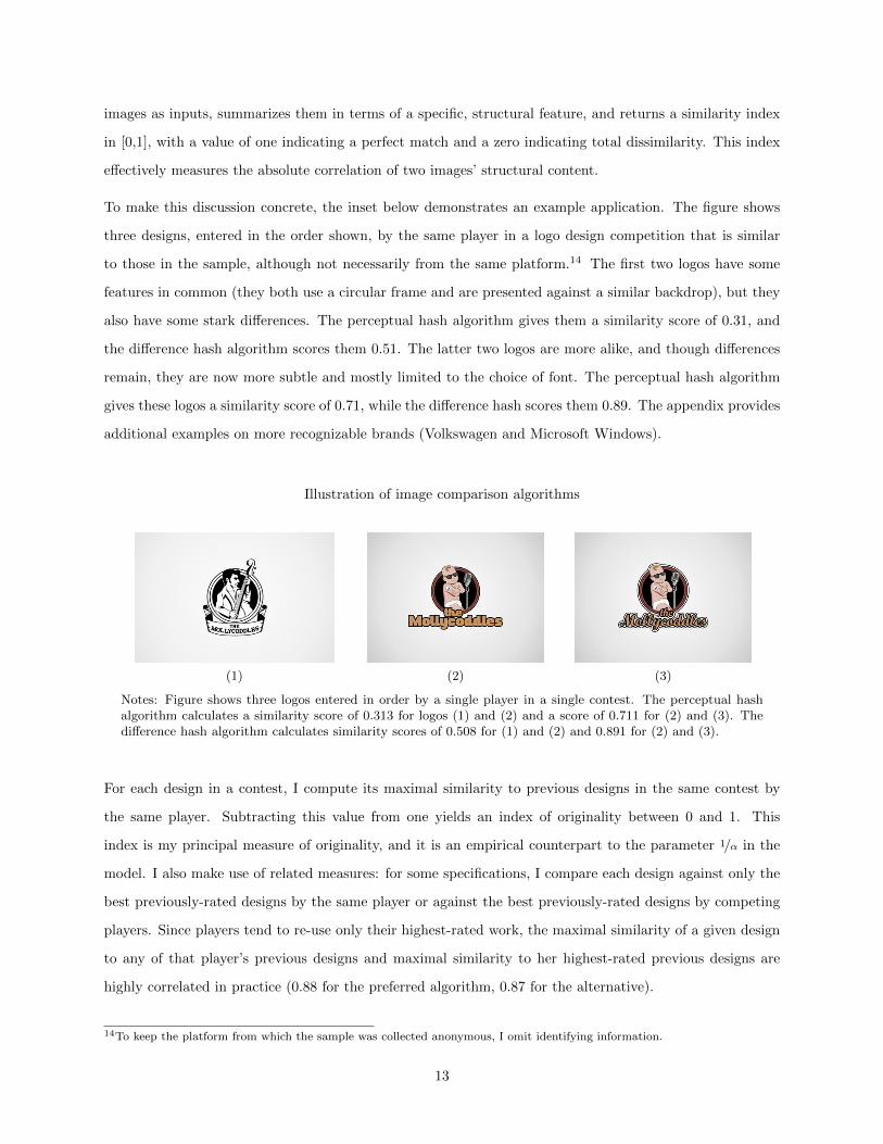
To make this discussion concrete, the inset below demonstrates an example application. The figure shows

three designs, entered in the order shown, by the same player in a logo design competition that is similar

to those in the sample, although not necessarily from the same platform.14 The first two logos have some

features in common (they both use a circular frame and are presented against a similar backdrop), but they

also have some stark differences. The perceptual hash algorithm gives them a similarity score of 0.31, and

the difference hash algorithm scores them 0.51. The latter two logos are more alike, and though differences

remain, they are now more subtle and mostly limited to the choice of font. The perceptual hash algorithm

gives these logos a similarity score of 0.71, while the difference hash scores them 0.89. The appendix provides

additional examples on more recognizable brands (Volkswagen and Microsoft Windows).

Illustration of image comparison algorithms

(1) (2) (3)

Notes: Figure shows three logos entered in order by a single player in a single contest. The perceptual hashalgorithm calculates a similarity score of 0.313 for logos (1) and (2) and a score of 0.711 for (2) and (3). Thedifference hash algorithm calculates similarity scores of 0.508 for (1) and (2) and 0.891 for (2) and (3).

For each design in a contest, I compute its maximal similarity to previous designs in the same contest by

the same player. Subtracting this value from one yields an index of originality between 0 and 1. This

index is my principal measure of originality, and it is an empirical counterpart to the parameter 1/α in the

model. I also make use of related measures: for some specifications, I compare each design against only the

best previously-rated designs by the same player or against the best previously-rated designs by competing

players. Since players tend to re-use only their highest-rated work, the maximal similarity of a given design

to any of that player’s previous designs and maximal similarity to her highest-rated previous designs are

highly correlated in practice (0.88 for the preferred algorithm, 0.87 for the alternative).

14To keep the platform from which the sample was collected anonymous, I omit identifying information.

13

Creativity can manifest in other ways. For example, players sometimes create and enter several designs at

once, and when doing so they can make each one similar to or distinct from the others. To capture this

phenomenon, I define “batches” of proximate designs entered into the same contest by a single player and

compute the maximum intra-batch similarity as a measure of creativity in batch work. Two designs are

proximate if they are entered within 15 minutes of each other, and a batch is a set of designs in which every

design in the set is proximate to another in the same set. Intra-batch similarity is an alternative – and

arguably better – measure of creative experimentation, reflecting players’ tendency to try minor variants of

the same concept or multiple concepts over a short period of time.

These measures are not without drawbacks or immune to debate. One drawback is that these algorithms

require substantial dimensionality reduction and thus provide only a coarse comparison between designs.

Concerns on this front are mitigated by the fact that the empirical results throughout the paper are similar

in sign, significance, and magnitude under two distinct algorithms. One might also question how well these

algorithms emulate human perception. The example here and in the appendix assuage this concern; more

generally, I have found these algorithms to be especially good at detecting designs that are plainly tweaks

to earlier work (by my perception) versus those that are not, which is the margin that matters most for this

paper. Appendix B discusses these and other related issues in greater detail.

2.1 Characteristics of the Sample

The average contest in the data lasts eight days, offers a $250 prize, and attracts 96 designs from 33 players

(Table 1). On average, 64 percent of designs are rated; less than three receive the top rating.

[Table 1 about here]

Among rated designs, and the median and modal rating is three stars (Table 2). Though fewer than four

percent of rated designs receive a 5-star rating, over 40 percent of all winning designs are rated five stars,

suggesting that these ratings convey substantial information about a design’s quality and odds of success.15

The website also provides formal guidance on the meaning of each star rating, which generates consistency

in their interpretation and use across different sponsors and contests.

[Table 2 about here]

Table 3 characterizes the similarity measures used in the empirical analysis. For each design in the sample,

I measure its maximal similarity to previous designs by the same player, previously-rated designs by the

15Another 33 percent of winning designs are rated 4 stars, and 24 percent are unrated.

14

same player, and previously-rated designs by the player’s competitors (all in the same contest). For every

design batch, I calculate the maximal similarity of any two designs in that batch. Note that the analysis of

intra-batch similarity is restricted to batches that are not missing any image files.

[Table 3 about here]

The designs themselves are available for 96 percent of submissions in the sample. The table shows that new

entries are on average more similar to that player’s own designs than her competitors’ designs, and that

designs in the same batch tend to be more similar to each other than to previous designs by even the same

player. But these averages mask more important patterns at the extremes. At the upper decile, designs

can be very similar to previous work by the same player (≈0.75 under the perceptual hash algorithm) or to

other designs in the same batch (0.91), but even the designs most similar to competing work are not all that

similar (0.27). At the lower end, designs can be original by all of these measures.

2.1.1 Correlations of contest characteristics with outcomes

To shed light on how these contests operate and how assorted levers affect outcomes of interest, Appendix

Table C.1 explores the relationship of contest outcomes with prize value, feedback, and other features. The

table borrows the large-sample data of Gross (2015), which uses a similar (but much larger) sample of logo

design contests from the same platform to study the effects of feedback on tournament outcomes. Though

the Gross (2015) dataset lacks the image files, it includes most of the other variables for these contests. As

the appendix also shows, this sample is broadly similar to that of the present paper.

The estimates in this table suggest that an extra $100 in prize value on average attracts an additional 13.3

players, 47.7 designs, and 0.1 designs per player and increases the odds that a retractable prize will be

awarded by 1.6 percent at the mean of all covariates. There is only a modest incremental effect of committed

prize dollars, likely because the vast majority of uncommitted prizes are awarded anyway. The effects of

feedback are also powerful: a sponsor who rates a high fraction of the designs in the contest will typically

see fewer players enter but receive more designs from the participating players and have a much higher

probability of finding a design it likes enough to award the prize. The effect of full feedback (relative to no

feedback) on the probability the prize is awarded is greater than that of a $1000 increase in the prize – a

more than quadrupling of the average and median prize in the sample.

15

2.1.2 Do ratings predict contest success? Estimating the success function

With the right data, the success function can be directly estimated. Recall from equation (1) that a design’s

latent value is a function of its rating and an i.i.d. extreme value error. In the data, there are five possible

ratings. This latent value can thus be flexibly specified with fixed effects for each rating (or no rating). The

success function can then be structurally estimated as a conditional logit model, using the observed win-lose

outcomes of every design in a large sample of contests. To formalize the empirical success function, let Rijk

denote the rating on design i by player j in contest k, and (in a slight abuse of notation) let Rijk = ∅ when

design ijk is unrated. The value of each design, νijk, can be written as follows:

νijk = γ∅1(Rijk = ∅) + γ11(Rijk = 1) + . . .+ γ51(Rijk = 5) + εijk ≡ ψijk + εijk (6)

This specification is closely related to the theoretical success function in equation (1), with the main difference

being a restricted, discrete domain for the feedback. As in the theoretical model, the sponsor is assumed to

select as winner the design with the highest value. In estimating the γ parameters, each sponsor’s choice

set of designs is assumed to satisfy I.I.A.; in principle, the submission of a design of any rating in a given

contest will reduce competing designs’ chances of winning proportionally. For contests with an uncommitted

prize, the choice set also includes an outside option of not awarding the prize, with value normalized to zero.

Letting Ijk be the set of designs by player j in contest k, and Ik be the set of all designs entered into that

same contest k, the empirical success function for player jk takes the following form:

Pr(j wins k) =

∑i∈Ijk e

ψijk∑i∈Ik e

ψik + 1(Uncommitted prize)

Gross (2015) estimates this model by maximum likelihood using a sample of 496,401 designs entered in 4,294

contests from the same setting. The results are reproduced in Appendix Table C.2.

Several patterns emerge from the exercise. The fixed effects are precisely estimated, and the estimated

value of a design is monotonically increasing in its rating. Only a 5-star design is on average preferred to

the outside option. To produce the same change in the success function generated by a five-star design, a

player would need 12 four-star designs, 137 three-star designs, or nearly 2,000 one-star designs, such that

competition at the top effectively only comes from other five-star designs. As a measure of fit, the model

correctly “predicts” the true winner relatively well, with the odds-on favorite winning almost half of all

contests in the sample. These results demonstrate that this simple model fits the data quite well and in

an intuitive way, suggesting that ratings provide considerable information about a player’s probability of

winning. The strong fit of the model also justifies the assumption that players can accurately assess these

16

odds: though players do not observe the ratings on specific competing designs, they are provided with the

distribution of ratings on their competitors’ designs, which makes it possible for players to invoke a simple

heuristic model such as the one estimated here in their decision-making.

2.2 Empirical Methods and Identification

I exploit variation in the level and timing of the sponsor’s ratings to estimate the effects of competition on

players’ creative choices. With timestamps on all activity, I can determine exactly what a player knows at

each point in time about the sponsor’s preference for her work and the competition she faces, and identify

the effects of ratings observed at the time of design. Identification is achieved by harnessing variation in the

information that players possess about their own and their competitors’ performance.

Formally, the identifying assumption is that there are no omitted factors correlated with observed feedback

that also affect choices. This assumption is supported by two pieces of evidence. First, the arrival of ratings

is unpredictable, such that the set of ratings observed at any point in time is effectively random: sponsors

are erratic, and it is difficult to know exactly when or how often a sponsor will log onto the site to rate

new entries, much less any single design. More importantly, players’ choices are uncorrelated with ratings

that were unobserved at the time, including forthcoming ratings and ratings on specific competing designs.

The thought experiment is to compare the actions of a player with a 5-star design under her belt before

learning the rating versus after, or with latent 5-star competition before finding out versus after – noting

that empirically, undisclosed information is as good as no information.16

To establish that feedback provision is unpredictable, I explore the relationship between feedback lags and

the rating given. In concept, sponsors may be quicker to rate the designs they like the most, to keep these

players engaged and improving their work, in which case players might infer the eventual ratings on their

designs from the time elapsed without any feedback. Players may also react to uncertainty generated by

delays in the provision of feedback, and if this uncertainty is related to the rating given, it would confound

my estimates. Empirical assessment of this question (in unreported results) reveals that this is not the case:

whether measured in hours or as a percent of the total contest duration, the lag between when a design is

entered and rated is statistically unrelated to its rating. The probability that a rated design was rated before

versus after the contest ends is similarly uncorrelated with the rating granted.

Evidence that choices are uncorrelated with unobserved feedback is presented in Section 3. As a first

check, I estimate the effects of observed ratings on originality both with and without controls for the player’s

16Though this setting may seem like a natural opportunity for a controlled experiment, the variation of interest is in the 5-starratings, which are sufficiently rare that a controlled intervention would require either unrealistic manipulation or an infeasiblylarge sample. I therefore exploit naturally-occurring variation for this study.

17

forthcoming ratings and find the results unchanged. For further evidence, I estimate the relationship between

forthcoming ratings and originality, finding that it is indistinguishable from zero. I also examine players’

tendency to imitate highly-rated competing designs and find no such patterns – either due to the copyright

protection mechanism or, more likely, because players simply do not know which competing designs are

highly rated (and thus which ones to imitate). The results collectively confirm that players respond only to

information they can access at the time of design and suggest that there are no omitted factors correlated

with feedback that would confound those effects.

3 Competition and Creative Choices

The theoretical predictions can now be put to the test. Section 3.1 (as well as Appendices D to F) provides a

battery of evidence that conditional on continued participation, competition induces high-performing players

to enter more original work than they otherwise would. The primary estimating equation in this part of the

paper is the following specification, with variants estimated throughout the analysis:

Similarityijk = β0 + β5 · 1(R̄ijk = 5) + β5c · 1(R̄ijk = 5) · 1(R̄−ijk = 5) + β5p · 1(R̄ijk = 5) · Pk

+

4∑r=2

βr · 1(R̄ijk = r) + γ · 1(R̄−ijk = 5) + Tijkλ+Xijkθ + ζk + ϕj + εijk

where Similarityijk is the maximal similarity of design ijk to any previous designs by player j in contest k;

R̄ijk is the highest rating player j has received in contest k prior to design ijk; R̄−ijk is the highest rating

player j’s competitors have received prior to design ijk; Pk is the prize in contest k (measured in $100s); Tijk

is fraction of the contest elapsed at the time design ijk is entered; Xijk is a vector of design-level controls,

consisting of the number of previous designs by the same player and competing players, and days remaining

in the contest; and ζk and ϕj are contest and player fixed effects, respectively.

It may be helpful to provide a roadmap to this part of the analysis in advance. In the first set of regressions,

I estimate the specification above. In the second set, I replace the dependent variable with the similarity to

that player’s best, previously-rated designs, and then within-batch similarity. The third set of regressions

examines the change in similarity to previously-rated designs, as a function of newly-received feedback.

The fourth set of regressions tests the aforementioned identifying assumption that players are not acting

on forthcoming information. The fifth set of regressions tests whether players imitate high-performing

competitors, which they should not be able to discern from the available information.

Section 3.2 provides the counterpart analysis examining the effects of competition on players’ tendency to

18

continue participating in or abandon the contest. The evidence substantiates the model’s second prediction:

that increasing competition can drive players to quit. The specifications in this section are similar to those

of the regressions testing originality. I estimate variants of the following model:

Abandonijk = β0 +

5∑r=1

βr · 1(R̄ijk = r) +

5∑r=1

δr · 1(R̄ijk = r) ·N−ijk

+ N−ijkδ + Tijkλ+Xijkθ + ζk + ϕj + εijk

where Abandonijk indicates that player j entered no additional designs in contest k after design ijk; N−ijk

is the number of five-star designs by player j’s competitors in contest k at the time of design ijk; and R̄ijk,

R̄−ijk, Tijk, Xijk, ζk, and ϕj retain their previous definitions. The precise moment at which each player

makes a decision to stop investing is impossible to measure, and I thus use inactivity as a proxy. In general,

this measure does not distinguish between a “wait and see” approach that ends with abandonment versus

abandonment immediately following design ijk. Since the end result is the same, the distinction is immaterial

for the purposes of this paper. Standard errors throughout the following subsections are clustered by player

to account for any within-player correlation in the error term.

3.1 Competition and Originality

3.1.1 Similarity of new designs to a player’s previous designs

I begin by studying players’ tendency to tweak any of their previous work in a contest. Table 4 provides

estimates from regressions of the maximal similarity of each design to previous designs by the same player on

indicators for the highest rating that player had previously received. All specifications include interactions of

the indicator for having received the top rating with (i) the prize value (in $100s) and (ii) a variable indicating

the presence of top-rated competition, as well as the fraction of the contest elapsed and contest and player

fixed effects. The even-numbered columns add the controls, which serve as alternative characterizations

of the contest’s progression. Columns (3) and (4) additionally control for future feedback on the player’s

earlier work; if players have contest-specific ability or other information unobserved by the researcher (e.g.,

sponsors’ written comments), it will be accounted for by these regressions.

[Table 4 about here]

The results are consistent across all specifications in the table. Players with the top rating enter designs

that are 0.3 points, or roughly one full standard deviation, more similar to previous work than players who

19

have only low feedback (or no feedback). Roughly one third of this effect is shaved off by the presence of

high-rated competition. With a highest observed rating of four stars, new designs are on average around 0.1

points more similar to previous work. This effect further attenuates as the best observed rating declines,

and it is indistinguishable from zero at a best observed rating of two stars.

In practice, players tend to tweak only their highest-rated designs. Table 5, columns (1) and (2) estimate a

variant on the first two columns of Table 4, regressing each design’s maximal similarity to the highest-rated

preceding designs by the same player on the same set of explanatory variables. Columns (3) and (4) invoke

the sample of design batches and the alternative measure of creativity: the maximal similarity of any two

designs in each batch. Columns (5) and (6) repeat this latter exercise, weighting observations of batches by

their size. All specifications control for contest and player fixed effects, and the table shows variants of the

regressions with versus without design- and batch-level covariates.

[Table 5 about here]

The results for the design-level regressions (Columns 1 and 2) are similar to but slightly stronger than those

of the previous table. Players with the top rating enter designs that are 0.35 points, or about 1.3 standard

deviations, more similar to their highest-rated work in that contest, but this effect is reduced by more than

half when there is top-rated competition. Players’ tendency to make tweaks on their best designs is again

monotonically decreasing in their highest prior rating.

Columns (3) to (6) demonstrate that competition has similar effects on originality within batches of designs.

When entering multiple designs at one time, the maximal similarity of any two designs in the batch declines

0.3 points, or approximately one standard deviation, for players with a top rating who face top-rated com-

petition, relative to those who do not. Top players facing competition are thus more likely to experiment

not only across batches but also within them. The consistency of the results demonstrates that they are not

sensitive to inclusion of controls or weighting batches by their size.

The regressions in Tables 4 and 5 use contest and player fixed effects to control for factors that are constant

within contests, across players or within players, across contests, but they do not control for factors that are

constant throughout a given contest for a given player, as doing so leaves too little variation for me to identify

the effects of feedback and competition. Such factors may nevertheless be confounding omitted variables.

For example, if players can sense their match to a particular contest, and change their behavior accordingly

throughout the contest, the estimated effects may be confounded by this unobserved self-selection – though

such concerns are in part relieved by the consistency of results in Table 4 controlling for forthcoming ratings.

The estimates in the previous tables additionally mask potential heterogeneity that may be present in players’

reactions to feedback and competition over the course of a contest.

20

Table 6 addresses these issues with a model in first differences. The dependent variable is the change in

designs’ similarity to the player’s best previously-rated work. This variable can take values in [-1,1], where

a value of 0 indicates that the given design is as similar to the player’s best preceding design as was the last

one she entered; a value of 1 indicates that the player transitioned fully from pioneering to recycling; and

a value of -1, the converse. The independent variables are changes in indicators for the highest rating the

player has received, with the usual interactions of the top rating with the prize and the presence of top-rated

competition. I estimate this model with assorted configurations of contest fixed effects, player fixed effects,

and controls to account for other reasons why players’ inclination to experiment may change over time,

though the results are not statistically different across these specifications.

[Table 6 about here]

The results provide the strongest evidence thus far on the effects of feedback and competition on creative

choices. When a player receives her first 5-star rating, her next design will be a near replica. The degree of

similarity increases by nearly 0.9 points, or three standard deviations. Top-rated competition shaves nearly

half of this effect. Given their magnitudes, these effects will be plainly visible to the naked eye (see the

earlier inset for an example of what they look like in practice). The effects of a new, best rating of 4-, 3-,

and 2-stars on originality attenuate monotonically, similar to previous results.

Interestingly, these regressions also find that new recipients of the top rating can also be induced to try new

designs with larger prizes. The model of Section 1 suggests a natural explanation for this result: large prizes

moderate the role of potentially higher costs in players’ decision-making. If original designs are more costly

(take more time or effort) than incremental tweaks, they may only be worth doing when the prize is large.

This is particularly the case for players with highly-rated work in the contest, given how the shape of and

movement along a player’s success function depends on the quality of her designs.

The appendix provides robustness checks and supplementary analysis. To confirm that these patterns are

not an artifact of the perceptual hash algorithm, Appendix D re-estimates the regressions in the preceding

tables using the difference hash algorithm to calculate similarity scores. The results are statistically and

quantitatively similar. In Appendix E, I split out the effects of competition by the number of top-rated

competing designs, finding no statistical differences between the effects of one versus more than one: all

effects of competition on originality are achieved by one high-quality competitor.

This latter result is especially important for ruling out an information-based story. The fact that other designs

received a 5-star rating might indicate that the sponsor has diverse preferences and that experimentation has

a higher likelihood of success than the player might otherwise believe. If this were the case, then originality

21

should continue to increase as 5-star competitors are revealed. That this is not the case suggests that the

effect is in fact the result of variation in incentives from competition.

The model suggests that similar dynamics should arise for players with 4-star ratings facing 4-star competition

when no higher ratings are granted, since only relative performance matters – though this result may only

arise towards the end of a contest, when the absence of higher ratings approaches finality. Appendix F tests

this prediction, finding similar patterns for 4-on-4 competition that strengthen over the course of a contest.

In unreported regressions, I also look for effects of 5-star competition on originality for players with only

4-star designs, and find attenuated effects that are negative but not significantly different from zero. I also

explore the effect of prize commitment on originality, since the sponsor’s outside option of not awarding the

prize is itself a competing alternative – one which according to the conditional logit estimates in Table C.2

is on average preferred to all but the highest-rated designs. The effect of prize commitment is not estimated

to be different from zero. I similarly test for effects of the presence of four-star competition on originality

for players with five-star designs, finding none. These results reinforce the perception that competition

effectively comes from designs with a contest’s highest rating.

3.1.2 Similarity of new designs to a player’s not-yet-rated designs

The identifying assumptions require that players are not acting on information that correlates with feedback

but is unobserved in the data. As a simple validation exercise, the regressions in Table 7 perform a placebo

test of whether originality is related to impending feedback. If an omitted determinant of creative choices

is correlated with the feedback, then it would appear as if originality responds to forthcoming ratings, but

if the identifying assumptions hold, we should only find zeros.

[Table 7 about here]

The specification in Column (1) regresses a design’s maximal similarity to the player’s best designs that have

not yet been but will eventually be rated on indicators for the ratings they later receive. I find no evidence

that designs’ originality is related to forthcoming ratings. Because a given design’s similarity to an earlier,

unrated design can be incidental if both are tweaks on a third design, Column (2) adds controls for similarity

to the best already-rated design. Column (3) allows these controls to vary with the rating received. As

a final check, I isolate the similarity to the unrated design that cannot be explained by similarity to the

third design in the form of a residual, and in Column (4) I regress these residuals on the same independent

variables. In all cases, I find no evidence that players systematically tweak designs with higher forthcoming

ratings. Feedback only relates to choices when observed in advance.

22

3.1.3 Imitation of competing designs

Though players can see a gallery of competing designs in the same contest, they see only the distribution of

feedback these designs have received – not the ratings provided to specific, competing entries – and should

therefore not be able to use this information to imitate highly-rated competitors. The regressions in Table

8 test this assumption by examining players’ tendency to imitate competitors.

The first two columns of the table provide estimates from regressions of similarity to the highest-rated design

by competing players on indicators for its rating. As in previous specifications, the top-rating indicator is

interacted with the prize and with an indicator for whether the player herself also has a top-rated design in

the contest. The latter columns repeat the exercise with first-differenced variants of the same specifications.

There is little evidence in this table that players imitate highly-rated competitors in any systematic way –

likely because they are simply unable to identify which competing designs are highly-rated. In unreported

results, I replace the left-hand side with imitation of any competing design and similarly find no effect. The

results establish that “creativity” in the presence of competition is not just imitation of competitors’ designs.

Appendix Table D.5 provides counterpart estimates using the difference hash algorithm, which suggest that

if anything, players tend to deviate away from competitors’ highly-rated work.

[Table 8 about here]

3.2 Competition and Abandonment

It remains to be seen how competition affects players’ decision to continue investing in the contest. In Table

9 I estimate the probability that a given design is a player’s final submission on the feedback and competition

that was observed at the time. As previously discussed, this measure of abandonment could reflect either

a simultaneous choice to abandon the project or a “wait and see” strategy that yields no further action –

although according to one designer who participates on this platform, it is often the case that players will

enter their final design knowing it is their final design and never look back. The specifications in the table

regress this measure of abandonment on indicators for the highest rating the player previously received,

interactions with the number of 5-star competing designs, the latter as a distinct regressor, the fraction of

the contest elapsed (a crucial control here), and other controls from previous tables.

[Table 9 about here]

Columns (1) to (3) estimate linear specifications with contest, player, and contest and player fixed effects.

Linear specifications are used in order to control for these fixed effects (especially player fixed effects), which

23

may not be estimated consistently in practice and could thus render the remaining estimates inconsistent in

a binary outcome model. Column (4) estimates a logit model with only the contest fixed effects. The linear

model with two-way fixed effects (in Column 3) is the preferred specification.

In all specifications, I find that players with higher ratings are more likely to continue investing than those

with lower ratings, but that high-rated competition drives them away. In the preferred linear probability

model in Column (3), I find that players with a top-rated design are more likely to subsequently enter more

designs, but this effect is offset by the presence of only a few 5-star competitors.

4 Does it Really Pay to Be Creative?

Why do the designers in these contests respond to competition by exploring new directions? In conversations

with creative professionals – including the panelists hired for the exercise below – many have asserted that

competition means that they need to “be bold” or “bring the ‘wow’ factor,” and that it induces them to

take creative risks. Gambling on a more radical, untested idea is thus a calculated and intentional choice.

The implicit assumption motivating this type of creative risk-taking both in the model and in practice is

that developing a new idea is a high-risk, high-return endeavor – the upside to doing so is what makes it

worthwhile. This assumption is common not only in research, but also in the public discourse on innovation

and entrepreneurship. Whether or not it is true is ultimately an empirical question.

A natural approach to answering this question in the setting of this paper is to examine the distribution of

sponsors’ ratings on original versus tweaked designs in the sample. To do so, I categorize designs as tweaks

if they have similarity to any earlier designs by the same player of 0.7 or higher and record the rating of the

design they are most similar to; I classify designs as original if their maximal similarity to earlier designs

by that player is 0.3 or below and record the highest rating the player had previously received.17 I then

compare the distribution of sponsors’ ratings on this subsample, conditioning on the rating of the tweaked

design (for tweaks) or the highest rating previously given to that player (for originals). The evidence suggests

that original designs outperform tweaks to designs with low ratings, but underperform tweaks of top-rated

designs, raising the question of why a player would deviate from her top-rated work.

The problem with this approach is that the observed outcomes are censored: it is impossible to observe the

fruits of a player’s creativity beyond the 5-star rating. With this top-code in place, original designs will

necessarily appear to underperform tweaks of 5-star designs – the sponsor’s rating can only go down. The

data are thus inadequate for evaluating the benefits to exploration for players at the top. To circumvent

17A player’s intentions are more ambiguous at intermediate values, which I accordingly omit from the exercise.

24

the top-code, I hired a panel of five professional graphic designers to independently assess all 316 designs

in my sample that were rated five stars by contest sponsors, and I look to the panelists’ ratings to evaluate

whether exploration is in fact high-risk, high-return.

Results from a Panel of Professional Designers

For this exercise, I hired five professional graphic designers at their regular rates to evaluate each design on

an extended scale. These ratings were collected though a custom web-based application in which designs

were presented in random order and panelists were limited to 100 ratings per day. With each design, the

panelist was provided the project title and client industry (excerpted from the source data) and instructed

to rate the “quality and appropriateness” of the given logo on a scale of 1 to 10.

Appendix G provides more detail on the survey procedure and shows the distribution of ratings from all

five panelists. One panelist (“Rater 5”) was particularly critical with his/her ratings and frequently ran up

against the lower bound. The mass around the lower bound was apparent after the first day of the survey

(i.e., after 100 ratings), and though I provide the results from this panelist in the appendix for the sake of

disclosure, the decision was made at that time to exclude these ratings from subsequent analysis. The results

are nevertheless robust to including ratings from this panelist above the lower bound.

To account for differences in the remaining panelists’ austerity, I first normalize their ratings by demeaning,

in essence removing rater fixed effects. For each design, I then compute summary statistics of the panelists’

ratings (mean, median, maximum, and s.d.). As an alternative approach to aggregating panelists’ ratings,

I also calculate each design’s score along the first principal component generated by a principal component

analysis. Collectively, these summary statistics characterize the distribution of opinion on a given design.

One way to think about them is as follows: if contest sponsors were randomly drawn from this population,

then the realized rating on the design would be a random draw from this distribution.

I identify designs as being tweaks or originals using the definitions above and then compare the level and

heterogeneity in panelists’ ratings on designs of each type. Table 10 provides the results. Designs classified

as tweaks are typically rated below-average, while those classified as original are typically above-average.

These patterns manifest for the PCA composite, mean, and median panelist ratings; the difference in all

three cases is on the order of around half of a standard deviation and is significant at the one percent level.

The maximum rating that a design receives from any of the panelists is also greater for originals, with the

difference significant at the one percent level. Yet so is the level of disagreement: the standard deviation

across panelists’ ratings on a given design is significantly greater for original designs than for tweaks. The

25

evidence thus appears to support the popular contention that radical innovation is both higher mean and

higher variance than incremental innovation, even at the top.18

[Table 10 about here]

5 When is Creativity Most Likely?

The reduced-form results establish that while competition can motivate high performers to experiment with

new ideas, too much competition will drive them out of the market altogether. How much is “too much”?

Given that the full effect of competition on originality is achieved by a single, high-quality competitor, and

that players are increasingly likely to stop investing as competition intensifies, it would be natural to conclude

that incentives for continued creativity peak in the presence of one top-rated competitor – just enough to

ensure that competition exists without further eroding returns to effort.

To formalize an answer to this question, I estimate a choice model in which with each submission, a player

selects from the three basic behaviors I observe in the data: (i) tweak and enter more designs, (ii) experiment

and enter more designs, and (iii) do either and subsequently abandon the contest. As before, I classify each

design as a tweak if its similarity to any earlier design by the same player is 0.7 or higher and original if its

maximal similarity to earlier designs by that player is 0.3 or lower.

Each action in this choice set is assumed to have latent utility uaijk, where i indexes submissions by player

j in contest k. I model this latent utility as a function of the player’s own ratings, her competitors’ ratings,

the fraction of the contest transpired, additional controls, and a logit error term:

uaijk = βa0 +

5∑r=1

βar · 1(R̄ijk = r) +

5∑r=1

γar · 1(R̄−ijk = r)

+ δa1 · 1(R̄ijk = 5)1(N−ijk = 1)

+ δa2 · 1(R̄ijk = 5)1(N−ijk = 2)

+ δa3 · 1(R̄ijk = 5)1(N−ijk ≥ 3)

+ Tijkλa +Xijkθ

a + εaijk, εaijk ∼ i.i.d. Type-I E.V.

The explanatory variables are defined as before: R̄ijk is the highest rating player j has received in contest k

prior to ijk, R̄−ijk is the highest rating on competing designs, N−ijk is the number of top-rated competing

designs, Tijk is the fraction of the contest already elapsed, and Xijk are controls.

18If anything, these differences may be understated. If a player enters the same design twice, the first would first be classifiedin this exercise as an original, and the second as a tweak, but they would receive the same rating from panelists. Excludingdesigns that are either tweaks of or tweaked by others in the sample does not affect the results.

26

I estimate the parameters by maximum likelihood using observed behavior. I then use the results to estimate

the probability that a player with a 5-star design takes each of the three actions near the end of a contest,

and to evaluate how these probabilities vary as the number of top-rated competitors increases from zero to

three or more (for the case of no 5-star competitors, I assume the highest rating on any competing design

is 4 stars). These probabilities are shown in Figure 3. Panel A plots the probability that the player tweaks;

Panel B, the probability that she experiments; and Panel C, the probability that she abandons the contest.

Bars around each point provide the associated 95 percent confidence interval.

[Figure 3 about here]

The probability that a high-performer tweaks one of her previous submissions (Panel A) peaks at 52 percent

when there are no 5-star competitors and is significantly lower with non-zero competition, with all differences

significant at the one percent level. The probability that the player actively experiments (Panel B) peaks at

52 percent with one 5-star competitor and is significantly lower with zero, two, or three 5-star competitors

(differences against zero and three significant at the one percent level; difference against two significant at

the ten percent level). Panel C shows that the probability of abandonment increases monotonically in the

level of competition, approaching 80 percent under heavy competition.

The inverted-U pattern can also be unearthed by other means. Taking advantage of the richness of the data,

an alternative is to model the same discrete choice as a function of a player’s contemporaneous probability

of winning, which can be computed using the conditional logit estimates in Table C.2, and the standard

controls. Figure 4 plots the results. The probability that a player tweaks her previous work (Panel A) is

maximized at around 0.7 when she is a strong favorite to win, and declines monotonically to zero as her

odds decline. The probability that the player experiments (Panel B) follows a distinct and highly significant

inverted-U pattern, peaking at approximately a one-half odds of winning. Finally, the probability that she

abandons (Panel C) increases from zero to around 0.8 as her odds of winning decline.

[Figure 4 about here]

Observed behavior thus appears to conform to the predictions of economic theory: when competition is low,

players are on the margin between exploration and exploitation, whereas when competition is high, they

straddle the margin between exploration and abandonment. The results of this execise also agree with the

reduced-form evidence, in finding that high-rated players are most likely to be creative when they encounter

precisely one highly-rated competitor. Panel B of each figure directly illustrates the inverted-U effect of

competition on creativity and serves as an empirical counterpart to Figure 2.

27

6 Implications and Conclusion

This paper combines theory, data from a sample of commercial logo design competitions, and new tools for

measuring the content of ideas to show that individuals’ incentives for creativity are greatest at intermediate

levels of competition. The results tie together literatures in bandit decision models and tournament compe-

tition, and they provide what is to my knowledge the most direct evidence yet available on how incentives

influence the intensity and direction of individuals’ creative production.

The results have direct implications for policies and programs meant to incentivize creativity, both in and

outside of the workplace. The foremost result is that the sharp incentives of prize competition can motivate

creative effort in a work environment, but that doing so requires striking a delicate balance in the intensity

of competition. In designing contracts for creative workers, managers would be keen to offer incentives for

high-quality work relative to that of peers or colleagues, in addition to the traditional strategy of establishing

a work environment with intrinsic motivators such as intellectual freedom, flexibility, and challenge. Another

advantage of the tournament-style incentive structure is that it incorporates tolerance for failure by allowing

players to recover from unsuccessful experimentation, which has been shown to be an important feature of

contracts for motivating innovation (e.g., Manso 2011, Ederer and Manso 2013).

In practice, the ‘Goldilocks’ level of competition preferred by a principal may be difficult to achieve, much

less determine. Finding it would likely require experimentation with the mechanism itself on the part of the

principal, such as by varying the prize, subsidizing or restricting entry, or eliminating non-preferred players

midway through the contest. In this paper, one high-quality competitor was found to be sufficient to induce

another high-quality player to explore new directions, and further increases in competition have the effect

of driving players away. As a rule of thumb for other settings, a good approximation may be to assume that

one competitor of similar ability is enough to elicit fresh thinking, but that having more than a few such

competitors is likely more harmful than helpful for motivating creative workers.

The results also have bearing on design of public incentives for R&D, which is itself a creative endeavor, and

the implementation of other policies (such as antitrust policy) undertaken with the intent of incentivizing

innovation. Although this paper is fundamentally about individuals, the theoretical framework can be

interpreted as firms competing in a winner-take-all market. This interpretation is not without some peril,

as markets are inherently more complex and dynamic than the model allows. The results nevertheless shed

light on the forces that define the relationship between competition and innovation, particularly in settings

where post-innovation rents are far larger than participants’ pre-existing rents.

Three concrete policy implications follow. The first is support for prize competition as a mechanism for gen-

erating innovation. While the focus of this paper is graphic design for marketing materials, it is conceivable

28

to think that similar forces might be at work in other settings, including R&D. For example, Scotchmer

(2004) recounts that in the 1970s, the U.S. Air Force issued an RFP for a fighter jet design whereby rival

companies were required to build prototypes and fly them in competitive demonstrations, with the top per-

former winning a contract – a process which ultimately led to the F-16 and F-18 fighter jets.19 This context

is particularly relevant today, as governments, private foundations, and firms are increasingly contracting

through R&D prizes and institutionalizing prize competition.20 The U.S. federal government now operates

a platform (Challenge.gov) where agencies can solicit creative solutions to technical and non-technical prob-

lems from the public; as of February 2014, the site listed hundreds of open competitions with prizes ranging

from status only (non-monetary) to upwards of 15 million dollars.

The second implication is an argument for monopoly and perfect competition potentially being equally

harmful to innovation in markets. According to the U.S. Horizontal Merger Guidelines (2010), “competition

often spurs firms to innovate,” and projected post-merger changes in the level of innovation is one of the

government’s criteria for evaluating mergers. The results of this paper suggest that a transition from no

competition to some competition increases incentives for radical innovation over more modest, incremental

improvements to existing technologies, but that returns to innovation can decline to zero in crowded or overly

competitive markets, leaving participants content with the status quo.

A final implication of the results in this paper is that contrary to the conventional wisdom that duplicated

R&D efforts are wasteful, simultaneous duplication may be ex-ante efficient: the competition of a horserace

may induce greater ingenuity, whose fruits might compensate for the deadweight loss of duplicated effort.

From a social welfare perspective, institutional policies prohibiting joint support of dueling research programs

would then be doing more harm than good. This corollary requires testing, but if true, it suggests not only

a fresh look at existing research on the welfare impacts of R&D, but potentially important changes to both

R&D policy and strategies for managing innovation in the firm.

19Looking further back in history, Brunt, Lerner, and Nicholas (2012) and Moser and Nicholas (2013) show that prize compe-titions by the Royal Agricultural Society of England in the 19th and 20th centuries and the 1851 Crystal Palace Exhibition(respectively) had a significant impact on the level and direction of inventive activity for years to come.

20See Williams (2012) for examples and an in-depth review of the literature on innovation inducement prizes.

29

References

Aghion, Philippe, Nick Bloom, Richard Blundell, Rachel Griffith, and Peter Howitt,

“Competition and Innovation: An Inverted-U Relationship,” Quarterly Journal of Economics, 2005,

120 (2), 701–728.

Akcigit, Ufuk and Qingmin Liu, “The Role of Information in Innovation and Competition,” 2014.

Working Paper.

Arrow, Kenneth J., “Economic Welfare and the Allocation of Resources for Invention,” in “The Rate

and Direction of Inventive Activity: Economic and Social Factors,” Princeton: Princeton University

Press, 1962.

Azoulay, Pierre, Joshua S. Graff Zivin, and Gustavo Manso, “Incentives and Creativity:

Evidence from the Academic Life Sciences,” RAND Journal of Economics, 2011, 42 (3), 527–554.

Baik, Kyung Hwan, “Effort Levels in Contests with Two Asymmetric Players,” Southern Economic

Journal, 1994, pp. 367–378.

Baye, Michael R. and Heidrun C. Hoppe, “The Strategic Equivalence of Rent-seeking, Innovation,

and Patent-race Games,” Games and Economic Behavior, 2003, 44 (2), 217–226.

Boudreau, Kevin J. and Karim R. Lakhani, “‘Open’ Disclosure of Innovations, Incentives and

Follow-on Reuse: Theory on Processes of Cumulative Innovation and a Field Experiment in Com-

putational Biology,” Research Policy, 2015, 44 (1).

, , and Michael Menietti, “Performance Responses To Competition Across Skill-Levels In Rank

Order Tournaments: Field Evidence and Implications For Tournament Design,” RAND Journal of

Economics. Forthcoming.

, Nicola Lacetera, and Karim R. Lakhani, “Incentives and Problem Uncertainty in Innovation

Contests: An empirical analysis,” Management Science, 2011, 57 (5), 843–863.

Brown, Jennifer, “Quitters Never Win: The (adverse) incentive effects of competing with superstars,”

Journal of Political Economy, 2011, 119 (5), 982–1013.

Brunt, Liam, Josh Lerner, and Tom Nicholas, “Inducement Prizes and Innovation,” Journal of

Industrial Economics, 2012, 60 (4), 657–696.

Cabral, Luis, “R&D Competition When Firms Choose Variance,” Journal of Economics & Manage-

ment Strategy, 2003, 12 (1), 139–150.

Charness, Gary and Daniela Grieco, “Creativity and Financial Incentives,” 2014. Working Paper.

Che, Yeon-Koo and Ian Gale, “Optimal Design of Research Contests,” American Economic Review,

2003, 93 (3), 646–671.

Cohen, Wesley M., “Fifty Years of Empirical Studies of Innovative Activity and Performance,”

Handbook of the Economics of Innovation, 2010, 1, 129–213.

Ederer, Florian, “Feedback and Motivation in Dynamic Tournaments,” Journal of Economics &

Management Strategy, 2010, 19 (3), 733–769.

30

and Gustavo Manso, “Is Pay-for-Performance Detrimental to Innovation?,” Management Science,

2013, 59 (7), 1496–1513.

Fudenberg, Drew, Richard Gilbert, Joseph Stiglitz, and Jean Tirole, “Preemption, Leapfrog-

ging, and Competition in Patent Races,” European Economic Review, 1983, 22 (1), 3–31.

Fullerton, Richard L. and R. Preston McAfee, “Auctioning Entry into Tournaments,” Journal

of Political Economy, 1999, 107 (3), 573–605.

Gilbert, Richard, “Looking for Mr. Schumpeter: Where are we in the competition-innovation de-

bate?,” in Adam B. Jaffe, Josh Lerner, and Scott Stern, eds., Innovation Policy and the Economy,

Volume 6, Cambridge: The MIT Press, 2006.

Gross, Daniel P., “Interim Feedback in Tournaments for Ideas: Trading Off Participation for Qual-

ity,” 2015. Working Paper.

Halac, Marina, Navin Kartik, and Qingmin Liu, “Contests for Experimentation,” 2015. Working

Paper.

Hendel, Igal and Yossi Spiegel, “Small Steps for Workers, a Giant Leap for Productivity,” American

Economic Journal: Economic Policy, 2014, 6 (1), 73–90.

Hennessey, Beth A. and Teresa M. Amabile, “Creativity,” Annual Review of Psychology, 2010,

61, 569–598.

Manso, Gustavo, “Motivating Innovation,” The Journal of Finance, 2011, 66 (5), 1823–1860.

Mokyr, Joel, The Lever of Riches: Technological Creativity and Economic Progress, New York:

Oxford University Press, 1990.

Moser, Petra and Tom Nicholas, “Prizes, Publicity and Patents: Non-monetary Awards as a

Mechanism to Encourage Innovation,” Journal of Industrial Economics, 2013, 61 (3), 763–788.

Rosen, Richard J., “Research and Development with Asymmetric Firm Sizes,” RAND Journal of

Economics, 1991, 22 (3), 411–429.

Schumpeter, Joseph A., Capitalism, Socialism, and Democracy, New York: Harper, 1942.

Sternberg, Robert J., Cognitive Psychology, 5th ed., Belmont: Wadsworth, 2008.

Taylor, Curtis R., “Digging for Golden Carrots: An analysis of research tournaments,” The American

Economic Review, 1995, pp. 872–890.

Terwiesch, Christian and Yi Xu, “Innovation Contests, Open Innovation, and Multiagent Problem

Solving,” Management Science, 2008, 54 (9), 1529–1543.

U.S. Dept. of Justice and Federal Trade Commission, Horizontal Merger Guidelines 2010.

Available at: http://www.justice.gov/atr/public/guidelines/hmg-2010.html.

Weitzman, Martin, “Hybridizing Growth Theory,” American Economic Review: Papers and Pro-

ceedings, 1996, 86 (2), 207–212.

, “Recombinant Growth,” Quarterly Journal of Economics, 1998, 113 (2), 331–360.

Williams, Heidi, “Innovation Inducement Prizes: Connecting Research to Policy,” Journal of Policy

Analysis and Management, 2012, 31 (3), 752–776.

31

Figure 1: Payoffs to each of exploration, exploitation, and abandonment (example)

0 20 40 60 80 100 1200

0.2

0.4

0.6

0.8

1

1.2

1.4

1.6

1.8

2x 10

6

Competition (µj)

Exp

ecte

d p

ayo

ff (

$s)

Abandonment preferred Exploration preferred

Exploitation preferred

Abandonment preferred

ExplorationExploitationAbandonment

Notes: Figure plots the payoffs to each of exploration, exploitation, and abandonment asa function of µj for the following parametrization:

βj1 = 10, q = 0.33, α = 9, c = 200k, d = 300k, P = 2m.

Figure 2: Payoff to exploration over next-best option (example)

0 20 40 60 80 100 120−3

−2.5

−2

−1.5

−1

−0.5

0

0.5

1x 10

5

Competition (µj)

Re

lative

pa

yo

ffs (

$s)

Region where exploration preferred

Exploration vs.abandonment Exploration vs.exploitation Exploration vs.next−best

Notes: Figure plots the incremental payoff to exploration over the next-best alternativeat each value of µj for the same parametrization as the previous figure. The inverted-Ueffect shown here is the core theoretical result of the paper.

32

Figure 3: Probability of tweaking, experimenting, and abandoning as a function of 5-star competition

0.0

0.2

0.4

0.6

0.8

1.0

0 1 2 3+

Num. 5−star competing designs

Tweak

Panel A

0.0

0.2

0.4

0.6

0.8

1.0

0 1 2 3+

Num. 5−star competing designs

Experiment

Panel B

0.0

0.2

0.4

0.6

0.8

1.0

0 1 2 3+

Num. 5−star competing designs

Abandon

Panel C

Notes: Figure plots the probability that a player who has at least one 5-star rating in a contest doesone of the following on (and after) a given submission: tweaks and then enters more designs (PanelA), experiments and then enters more designs (Panel B), or abandons the contest (Panel C). Thebars around each point provide the associated 95 percent confidence interval.

The figure establishes that experimentation follows an inverted-U pattern over competition in thedata. This non-monotonicity appears to arise due to dynamics posited by the theory: when theprobability of winning is high, players are on the margin between tweaks and experimentation (theincentive compatibility constraint, Panels A and B); when it is low, they are on the margin betweenexperimentation and abandonment (participation constraint, Panels B and C).

Figure 4: Probability of tweaking, experimenting, and abandoning as a function of Pr(Win)

0.0

0.2

0.4

0.6

0.8

0.00.20.40.60.81.0

Win probability

Tweak

Panel A

0.0

0.2

0.4

0.6

0.8

0.00.20.40.60.81.0

Win probability

Experiment

Panel B

0.0

0.2

0.4

0.6

0.8

0.00.20.40.60.81.0

Win probability

Abandon

Panel C

Notes: Figure plots the probability that a player does one of the following on (and after) a givensubmission, as a function of their contemporaneous win probability: tweaks and then enters moredesigns (Panel A), experiments and then enters more designs (Panel B), or abandons the contest(Panel C). These probabilities are estimated as described in the text, and the bars around eachpoint provide the associated 95 percent confidence interval.

33

Table 1: Characteristics of contests in the sample

Variable N Mean SD P25 P50 P75

Contest length (days) 122 8.52 3.20 7 7 11Prize value (US$) 122 247.57 84.92 200 200 225No. of players 122 33.20 24.46 19 26 39No. of designs 122 96.38 80.46 52 74 107

5-star designs 122 2.59 4.00 0 1 44-star designs 122 12.28 12.13 3 9 183-star designs 122 22.16 25.33 6 16 282-star designs 122 17.61 25.82 3 10 221-star designs 122 12.11 25.24 0 2 11Unrated designs 122 29.62 31.43 7 19 40

Number rated 122 66.75 71.23 21 50 83Fraction rated 122 0.64 0.30 0.4 0.7 0.9Prize committed 122 0.56 0.50 0.0 1.0 1.0Prize awarded 122 0.85 0.36 1.0 1.0 1.0

Notes: Table reports descriptive statistics for the contests. “Fraction rated” refers to thefraction of designs in each contest that gets rated. “Prize committed” indicates whetherthe contest prize is committed to be paid (vs. retractable). “Prize awarded” indicateswhether the prize was awarded. The fraction of contests awarded awarded subsumes thefraction committed, since committed prizes are always awarded.

Table 2: Distribution of ratings (rated designs only)

1-star 2-star 3-star 4-star 5-star Total

Count 1,478 2,149 2,703 1,498 316 8,144Percent 18.15 26.39 33.19 18.39 3.88 100

Notes: Table tabulates rated designs by rating. 69.3 percent of designsin the sample are rated by sponsors on a 1-5 scale. The site providesguidance on the meaning of each rating, which introduces consistencyin the interpretation of ratings across contests.

Table 3: Similarity to preceding designs by same player and competitors, and intra-batch similarity

Panel A. Using preferred algorithm: Perceptual HashVariable N Mean SD P10 P50 P90

Max. similarity to any of own preceding designs 5,075 0.32 0.27 0.05 0.22 0.77Max. similarity to best of own preceding designs 3,871 0.28 0.27 0.03 0.17 0.72Max. similarity to best of oth. preceding designs 9,709 0.14 0.1 0.04 0.13 0.27Maximum intra-batch similarity 1,987 0.45 0.32 0.05 0.41 0.91

Panel B. Using alternative algorithm: Difference HashVariable N Mean SD P10 P50 P90

Max. similarity to any of own preceding designs 5,075 0.58 0.28 0.16 0.62 0.94Max. similarity to best of own preceding designs 3,871 0.52 0.3 0.09 0.54 0.93Max. similarity to best of oth. preceding designs 9,709 0.33 0.21 0.09 0.29 0.63Maximum intra-batch similarity 1,987 0.69 0.28 0.23 0.77 0.98

Notes: Table reports summary statistics on designs’ similarity to previously entered designs (both own andcompeting). Pairwise similarity scores are calculated as described in the text and available for all designswhose digital image could be obtained (96% of entries; refer to the text for an explanation of missing images).The “best” preceding designs are those with the most positive feedback provided prior to the given design.Intra-batch similarity is calculated as the similarity of designs in a given batch to each other, where a designbatch is defined to be a set of designs entered by a single player in which each design was entered within 15minutes of another design in the set. This grouping captures players’ tendency to submit multiple designs atonce, which are often similar with minor variations on a theme.

34

Table 4: Similarity to any of player’s previous designs

(1) (2) (3) (4)Player’s prior best rating==5 0.286*** 0.277*** 0.288*** 0.276***

(0.085) (0.087) (0.084) (0.087)* 1+ competing 5-stars -0.110* -0.118** -0.105* -0.109*

(0.058) (0.059) (0.058) (0.058)* prize value ($100s) -0.011 -0.021 -0.013 -0.025

(0.028) (0.028) (0.028) (0.028)Player’s prior best rating==4 0.100*** 0.077*** 0.100*** 0.076***

(0.017) (0.017) (0.017) (0.018)Player’s prior best rating==3 0.039*** 0.029** 0.039*** 0.027*

(0.014) (0.014) (0.014) (0.014)Player’s prior best rating==2 -0.004 -0.009 -0.003 -0.011

(0.020) (0.020) (0.020) (0.020)One or more competing 5-stars -0.011 -0.016 -0.010 -0.017

(0.021) (0.022) (0.021) (0.022)Pct. of contest elapsed 0.037 -0.097 0.037 -0.096

(0.028) (0.073) (0.028) (0.073)Constant 0.295 0.414** 0.293 0.407**

(0.179) (0.195) (0.179) (0.196)N 5075 5075 5075 5075R2 0.47 0.47 0.47 0.47Controls No Yes No YesContest FEs Yes Yes Yes YesPlayer FEs Yes Yes Yes YesForthcoming ratings No No Yes Yes

Notes: Table shows the effects of feedback on originality. Observations are designs. Depen-dent variable is a continuous measure of a design’s maximal similarity to previous entries inthe same contest by the same player, taking values in [0,1], where a value of 1 indicates thedesign is identical to another. The mean value of this variable is 0.32 (s.d. 0.27). Columns(2) and (4) control for days remaining and number of previous designs by the player and hercompetitors. Columns (3) and (4) additionally control for the best forthcoming rating on theplayer’s not-yet-rated designs. Similarity scores in this table are calculated using a percep-tual hash algorithm. Preceding designs/ratings are defined to be those entered/provided atleast 60 minutes prior to the given design. *, **, *** represent significance at the 0.1, 0.05,and 0.01 levels, respectively. Standard errors clustered by player in parentheses.

35

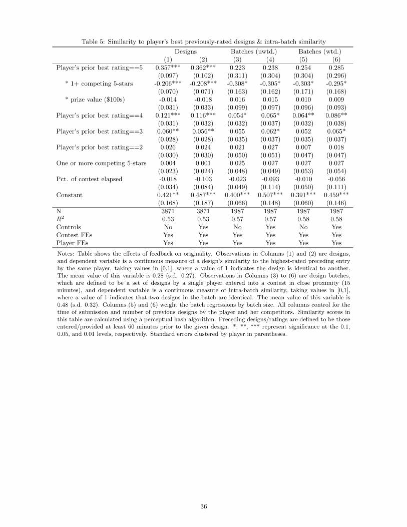
Table 5: Similarity to player’s best previously-rated designs & intra-batch similarity

Designs Batches (uwtd.) Batches (wtd.)(1) (2) (3) (4) (5) (6)

Player’s prior best rating==5 0.357*** 0.362*** 0.223 0.238 0.254 0.285(0.097) (0.102) (0.311) (0.304) (0.304) (0.296)

* 1+ competing 5-stars -0.206*** -0.208*** -0.308* -0.305* -0.303* -0.295*(0.070) (0.071) (0.163) (0.162) (0.171) (0.168)

* prize value ($100s) -0.014 -0.018 0.016 0.015 0.010 0.009(0.031) (0.033) (0.099) (0.097) (0.096) (0.093)

Player’s prior best rating==4 0.121*** 0.116*** 0.054* 0.065* 0.064** 0.086**(0.031) (0.032) (0.032) (0.037) (0.032) (0.038)

Player’s prior best rating==3 0.060** 0.056** 0.055 0.062* 0.052 0.065*(0.028) (0.028) (0.035) (0.037) (0.035) (0.037)

Player’s prior best rating==2 0.026 0.024 0.021 0.027 0.007 0.018(0.030) (0.030) (0.050) (0.051) (0.047) (0.047)

One or more competing 5-stars 0.004 0.001 0.025 0.027 0.027 0.027(0.023) (0.024) (0.048) (0.049) (0.053) (0.054)

Pct. of contest elapsed -0.018 -0.103 -0.023 -0.093 -0.010 -0.056(0.034) (0.084) (0.049) (0.114) (0.050) (0.111)

Constant 0.421** 0.487*** 0.400*** 0.507*** 0.391*** 0.459***(0.168) (0.187) (0.066) (0.148) (0.060) (0.146)

N 3871 3871 1987 1987 1987 1987R2 0.53 0.53 0.57 0.57 0.58 0.58Controls No Yes No Yes No YesContest FEs Yes Yes Yes Yes Yes YesPlayer FEs Yes Yes Yes Yes Yes Yes

Notes: Table shows the effects of feedback on originality. Observations in Columns (1) and (2) are designs,and dependent variable is a continuous measure of a design’s similarity to the highest-rated preceding entryby the same player, taking values in [0,1], where a value of 1 indicates the design is identical to another.The mean value of this variable is 0.28 (s.d. 0.27). Observations in Columns (3) to (6) are design batches,which are defined to be a set of designs by a single player entered into a contest in close proximity (15minutes), and dependent variable is a continuous measure of intra-batch similarity, taking values in [0,1],where a value of 1 indicates that two designs in the batch are identical. The mean value of this variable is0.48 (s.d. 0.32). Columns (5) and (6) weight the batch regressions by batch size. All columns control for thetime of submission and number of previous designs by the player and her competitors. Similarity scores inthis table are calculated using a perceptual hash algorithm. Preceding designs/ratings are defined to be thoseentered/provided at least 60 minutes prior to the given design. *, **, *** represent significance at the 0.1,0.05, and 0.01 levels, respectively. Standard errors clustered by player in parentheses.

36

Table 6: Change in similarity to player’s best previously-rated designs

(1) (2) (3) (4) (5) (6)∆(Player’s best rating==5) 0.878*** 0.927*** 0.914*** 0.885*** 0.929*** 0.924***

(0.170) (0.203) (0.205) (0.171) (0.202) (0.205)* 1+ competing 5-stars -0.412*** -0.418*** -0.427*** -0.414*** -0.418*** -0.429***

(0.125) (0.144) (0.152) (0.125) (0.144) (0.152)* prize value ($100s) -0.094** -0.114** -0.107** -0.096** -0.114** -0.110**

(0.039) (0.049) (0.047) (0.040) (0.049) (0.048)∆(Player’s best rating==4) 0.282*** 0.268*** 0.276*** 0.283*** 0.270*** 0.279***

(0.065) (0.073) (0.079) (0.065) (0.073) (0.079)∆(Player’s best rating==3) 0.151*** 0.135** 0.137** 0.151*** 0.136** 0.138**

(0.058) (0.065) (0.069) (0.058) (0.065) (0.069)∆(Player’s best rating==2) 0.082* 0.063 0.059 0.082* 0.063 0.059

(0.046) (0.052) (0.056) (0.046) (0.053) (0.057)One or more competing 5-stars -0.003 -0.003 0.004 -0.002 -0.004 0.003

(0.015) (0.014) (0.025) (0.015) (0.014) (0.026)Pct. of contest elapsed 0.009 0.017 0.004 -0.035 0.007 -0.048

(0.018) (0.024) (0.030) (0.043) (0.048) (0.074)Constant -0.017* -0.022 0.029 0.025 -0.015 0.060

(0.010) (0.014) (0.059) (0.040) (0.037) (0.077)N 2694 2694 2694 2694 2694 2694R2 0.05 0.11 0.14 0.05 0.11 0.14Controls No No No Yes Yes YesContest FEs Yes No Yes Yes No YesPlayer FEs No Yes Yes No Yes Yes

Notes: Table shows the effects of feedback on originality. Observations are designs. Dependent variable is acontinuous measure of the change in designs’ similarity to the highest-rated preceding entry by the same player,taking values in [-1,1], where a value of 0 indicates that the player’s current design is as similar to her bestpreceding design as was her previous design, and a value of 1 indicates that the player transitioned fully fromexperimenting to copying (and a value of -1, the converse). The mean value of this variable is 0.00 (s.d. 0.23).Columns (4) to (6) control for days remaining and number of previous designs by the player and competitors.Similarity scores in this table are calculated using a perceptual hash algorithm. Preceding designs/ratings aredefined to be those entered/provided at least 60 minutes prior to the given design. *, **, *** represent significanceat the 0.1, 0.05, and 0.01 levels, respectively. Standard errors clustered by player in parentheses.

37

Table 7: Similarity to player’s best not-yet-rated designs (placebo test)

Similarity to forthcoming Residual(1) (2) (3) (4)

Player’s best forthcoming rating==5 0.007 -0.084 -0.105 -0.113(0.169) (0.136) (0.151) (0.122)

* 1+ competing 5-stars -0.094 0.032 0.027 0.035(0.099) (0.056) (0.066) (0.062)

* prize value ($100s) -0.003 0.015 0.021 0.018(0.031) (0.025) (0.027) (0.025)

Player’s best forthcoming rating==4 0.039 0.051 0.049 0.034(0.066) (0.096) (0.094) (0.095)

Player’s best forthcoming rating==3 0.080 0.049 0.051 0.036(0.052) (0.088) (0.088) (0.088)

Player’s best forthcoming rating==2 0.030 -0.010 -0.007 -0.014(0.049) (0.093) (0.094) (0.095)

One or more competing 5-stars -0.080 -0.013 -0.010 -0.013(0.097) (0.110) (0.117) (0.119)

Pct. of contest elapsed 0.016 -0.502 -0.466 -0.468(0.242) (0.478) (0.462) (0.497)

Constant 0.223 0.637 0.716 0.299(0.321) (0.559) (0.619) (0.532)

N 1147 577 577 577R2 0.68 0.83 0.83 0.67Controls Yes Yes Yes YesContest FEs Yes Yes Yes YesPlayer FEs Yes Yes Yes Yes

Notes: Table provides a placebo test of the effects of future feedback on originality. Obser-vations are designs. Dependent variable in Columns (1) to (3) is a continuous measure of adesign’s similarity to the best design that the player has previously entered that has yet tobut will eventually be rated, taking values in [0,1], where a value of 1 indicates that the twodesigns are identical. The mean value of this variable is 0.26 (s.d. 0.25). Under the identify-ing assumption that future feedback is unpredictable, current choices should be unrelated toforthcoming ratings. Note that a given design’s similarity to an earlier, unrated design canbe incidental if they are both tweaks on a rated third design. To account for this possibility,Column (2) controls for the given and unrated designs’ similarity to the best previously-rateddesign. Column (3) allows these controls to vary with the highest rating previously received.Dependent variable in Column (4) is the residual from a regression of the dependent variablein the previous columns on these controls. These residuals will be the subset of a given de-sign’s similarity to the unrated design that is not explained by jointly-occurring similarity toa third design. All columns control for days remaining and number of previous designs by theplayer and her competitors. Similarity scores in this table are calculated using a perceptualhash algorithm. Preceding designs/ratings are defined to be those entered/provided at least 60minutes prior to the given design. *, **, *** represent significance at the 0.1, 0.05, and 0.01levels, respectively. Standard errors clustered by player in parentheses.

38

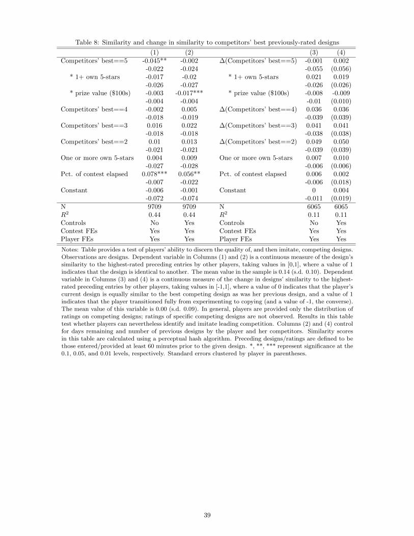
Table 8: Similarity and change in similarity to competitors’ best previously-rated designs

(1) (2) (3) (4)Competitors’ best==5 -0.045** -0.002 ∆(Competitors’ best==5) -0.001 0.002

-0.022 -0.024 -0.055 (0.056)* 1+ own 5-stars -0.017 -0.02 * 1+ own 5-stars 0.021 0.019

-0.026 -0.027 -0.026 (0.026)* prize value ($100s) -0.003 -0.017*** * prize value ($100s) -0.008 -0.009

-0.004 -0.004 -0.01 (0.010)Competitors’ best==4 -0.002 0.005 ∆(Competitors’ best==4) 0.036 0.036

-0.018 -0.019 -0.039 (0.039)Competitors’ best==3 0.016 0.022 ∆(Competitors’ best==3) 0.041 0.041

-0.018 -0.018 -0.038 (0.038)Competitors’ best==2 0.01 0.013 ∆(Competitors’ best==2) 0.049 0.050

-0.021 -0.021 -0.039 (0.039)One or more own 5-stars 0.004 0.009 One or more own 5-stars 0.007 0.010

-0.027 -0.028 -0.006 (0.006)Pct. of contest elapsed 0.078*** 0.056** Pct. of contest elapsed 0.006 0.002

-0.007 -0.022 -0.006 (0.018)Constant -0.006 -0.001 Constant 0 0.004

-0.072 -0.074 -0.011 (0.019)N 9709 9709 N 6065 6065R2 0.44 0.44 R2 0.11 0.11Controls No Yes Controls No YesContest FEs Yes Yes Contest FEs Yes YesPlayer FEs Yes Yes Player FEs Yes Yes

Notes: Table provides a test of players’ ability to discern the quality of, and then imitate, competing designs.Observations are designs. Dependent variable in Columns (1) and (2) is a continuous measure of the design’ssimilarity to the highest-rated preceding entries by other players, taking values in [0,1], where a value of 1indicates that the design is identical to another. The mean value in the sample is 0.14 (s.d. 0.10). Dependentvariable in Columns (3) and (4) is a continuous measure of the change in designs’ similarity to the highest-rated preceding entries by other players, taking values in [-1,1], where a value of 0 indicates that the player’scurrent design is equally similar to the best competing design as was her previous design, and a value of 1indicates that the player transitioned fully from experimenting to copying (and a value of -1, the converse).The mean value of this variable is 0.00 (s.d. 0.09). In general, players are provided only the distribution ofratings on competing designs; ratings of specific competing designs are not observed. Results in this tabletest whether players can nevertheless identify and imitate leading competition. Columns (2) and (4) controlfor days remaining and number of previous designs by the player and her competitors. Similarity scoresin this table are calculated using a perceptual hash algorithm. Preceding designs/ratings are defined to bethose entered/provided at least 60 minutes prior to the given design. *, **, *** represent significance at the0.1, 0.05, and 0.01 levels, respectively. Standard errors clustered by player in parentheses.

39

Table 9: Abandonment after a given design, as function of feedback and competition

Dependent variable: Abandon after given design(1) (2) (3) (4)

Linear Linear Linear LogitPlayer’s prior best rating==5 -0.013 -0.169*** -0.146*** -0.062

(0.034) (0.055) (0.044) (0.175)* competing 5s 0.012* 0.023*** 0.023*** 0.059**

(0.007) (0.009) (0.008) (0.030)Player’s prior best rating==4 -0.056*** -0.114*** -0.091*** -0.233***

(0.016) (0.023) (0.023) (0.082)* competing 5s 0.015*** 0.022*** 0.021*** 0.087***

(0.005) (0.008) (0.008) (0.026)Player’s prior best rating==3 -0.026* -0.029 -0.004 -0.060

(0.015) (0.019) (0.019) (0.071)* competing 5s 0.014** 0.022*** 0.018** 0.066**

(0.007) (0.008) (0.008) (0.028)Player’s prior best rating==2 -0.023 0.011 0.029 -0.052

(0.022) (0.026) (0.027) (0.107)* competing 5s 0.009 0.031** 0.026* 0.044

(0.010) (0.014) (0.013) (0.044)Player’s prior best rating==1 -0.027 0.050 0.059 -0.077

(0.035) (0.038) (0.038) (0.168)* competing 5s -0.025* -0.009 -0.018 -0.113*

(0.013) (0.019) (0.019) (0.065)Competing 5-star designs 0.009** -0.006* 0.003 0.046**

(0.004) (0.003) (0.005) (0.018)Pct. of contest elapsed 0.214*** 0.401*** 0.383*** 1.022***

(0.049) (0.042) (0.058) (0.229)Constant 0.222*** 0.085** 0.021 -1.423***

(0.044) (0.034) (0.100) (0.334)N 11758 11758 11758 11758R2 0.07 0.26 0.28Controls Yes Yes Yes YesContest FEs Yes No Yes YesPlayer FEs No Yes Yes No

Notes: Table shows the effects of feedback and competition at the time a design is entered onthe probability that player subsequently continues to participate (by entering more designs) versusabandons the contest. Observations are designs. Dependent variable in all columns is an indicatorfor whether the player stops participating. Columns (1) to (3) estimate linear models with fixedeffects; Column (4) estimates a logit model without player fixed effects, which could render theresults inconsistent. All columns control for days remaining and number of previous designs by theplayer and her competitors. Results are qualitatively similar under a proportional hazards model.*, **, *** represent significance at the 0.1, 0.05, and 0.01 levels, respectively. Standard errorsclustered by player in parentheses.

40

Table 10: Normalized panelist ratings on tweaks vs. original designs

Outcomes for: Diff. inMetric Tweaks Originals means

PCA score of -0.45 0.18 0.64***panelist ratings (0.21) (0.15) p=0.008

Average rating -0.45 0.22 0.67***by panelists (0.20) (0.14) p=0.004

Median rating -0.46 0.23 0.69***by panelists (0.21) (0.15) p=0.005

Max rating 1.08 1.99 0.91***by panelists (0.22) (0.17) p=0.001

Disagreement (s.d.) 1.34 1.59 0.25**among panelists (0.10) (0.07) p=0.019

Notes: Table compares professional graphic designers’ ratings ontweaks and original designs that received a top rating from contestsponsors. Panelists’ ratings were demeaned prior to analysis. ThePCA score refers to a design’s score along the first component froma principal component component analysis of panelists’ ratings. Theother summary measures are the mean, median, max, and s.d. of pan-elists’ ratings on a given design. A design is classified as a tweak ifits maximal similarity to any previous design by that player is greaterthan 0.7 and as original if it is less than 0.3. Standard errors in paren-theses are provided below each mean, and results from a one-sidedtest of equality of means is provided to the right. *, **, *** indicatesignificance at the 0.1, 0.05, and 0.01 levels, respectively. Similarityscores calculated using perceptual hash algorithm. Results are robustto both algorithms and alternative cutoffs for originality.

41

Appendix for Online Publication

A Proofs of Theorems and Additional Figures

Lemma 1: The agent’s gains to exploration over abandonment are increasing and concave in µ when µ is small

and decreasing and convex when µ is large. The gains are zero when µ = 0 and approach zero from above as

µ→∞, holding β1 fixed.

Proof:

Part (i): Low µ. As µ −→ 0:

qF(βH2)

+ (1− q)F(βL2)− F (0) = q

((1 + α)β1

(1 + α)β1 + µ

)+ (1− q)

( (1 + 1

α

)β1(

1 + 1α

)β1 + µ

)−(

β1β1 + µ

)

−→ q

((1 + α)β1(1 + α)β1

)+ (1− q)

((1 + 1

α

)β1(

1 + 1α

)β1

)−(β1β1

)= q + (1− q)− 1 = 0

∂

∂µ

[qF(βH2)

+ (1− q)F(βL2)− F (0)

]= q

(− (1 + α)β1

((1 + α)β1 + µ)2

)+ (1− q)

(−(1 + 1

α

)β1((

1 + 1α

)β1 + µ

)2)

+β1

(β1 + µ)2

−→ q

(−1

(1 + α)β0

)+ (1− q)

(−1(

1 + 1α

)β0

)+

1

β0

=−q(1 + 1

α

)− (1− q) (1 + α) + (1 + α)

(1 + 1

α

)(1 + α)

(1 + 1

α

)β1

=−(q + 1

αq)− (1− q + α− αq) +

(1 + α+ 1

α + 1)

(1 + α)(1 + 1

α

)β1

=αq − 1

αq + α+ 1α

(1 + α)(1 + 1

α

)β1

=

(α2 − 1

)q +

(1 + α2

)(1 + α)

2β1

−→ 0+

∂2

∂µ2

[qF(βH2)

+ (1− q)F(βL2)− F (0)

]= q

(2 (1 + α)β1

((1 + α)β1 + µ)3

)+ (1− q)

(2(1 + 1

α

)β1((

1 + 1α

)β1 + µ

)3)− 2β1

(β1 + µ)3 ,

numerator −→(q · (1 + α)

(1 + 1

α

)3+ (1− q) ·

(1 + 1

α

)(1 + α)

3 − (1 + α)3 (

1 + 1α

)3)2β7

1 < 0

1

Part (ii): High µ. As µ −→∞:

qF(βH2)

+ (1− q)F(βL2)− F (0) = q

((1 + α)β1

(1 + α)β1 + µ

)+ (1− q)

( (1 + 1

α

)β1(

1 + 1α

)β1 + µ

)−(

β1β1 + µ

)−→ 1

µ

(q (1 + α)β1 + (1− q)

(1 +

1

α

)β1 − β1

)=

1

µβ1

(αq − 1

αq +

1

α

)=

1

αµβ1((α2 − 1

)q + 1

)−→ 0+

∂

∂µ

[qF(βH2)

+ (1− q)F(βL2)− F (0)

]= q

(− (1 + α)β1

((1 + α)β1 + µ)2

)+ (1− q)

(−(1 + 1

α

)β1((

1 + 1α

)β1 + µ

)2)

+β1

(β1 + µ)2

−→ 1

µ2

(−q (1 + α)β1 − (1− q)

(1 +

1

α

)β1 + β1

)=

1

µ2β1

(− (q + αq)−

(1− q +

1

α− 1

αq

)+ 1

)=

1

µ2β1

(−αq +

1

αq − 1

α

)=

1

αµ2β1(−(α2 − 1

)q − 1

)−→ 0−

∂2

∂µ2

[qF(βH2)

+ (1− q)F(βL2)− F (0)

]= q

(2 (1 + α)β1

((1 + α)β1 + µ)3

)+ (1− q)

(2(1 + 1

α

)β1((

1 + 1α

)β1 + µ

)3)− 2β1

(β1 + µ)3 ,

numerator −→(q · (1 + α) + (1− q) ·

(1 + 1

α

)− 1)

2β1µ6 > 0

Taken together, these asymptotics generate a curve with the shape described.

Proposition 1: For all values of q, there exists a unique level of competition µ∗1 at which the gains to exploration,

relative to abandonment, are maximized.

Proof: Existence follows from lemma and continuity of the success function. Since the difference of the success

function under exploration and abandonment is quadratic in µ, it has at most two real roots, one of which is shown

below to be zero, the other of which is shown to be negative. Given the shape described by the lemma, the value

at which this difference is maximized must be unique.

2

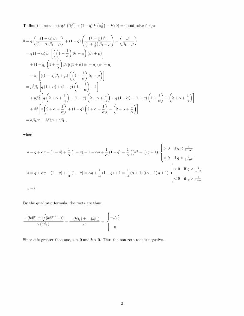
To find the roots, set qF(βH2)

+ (1− q)F(βL2)− F (0) = 0 and solve for µ:

0 = q

((1 + α)β1

(1 + α)β1 + µ

)+ (1− q)

( (1 + 1

α

)β1(

1 + 1α

)β1 + µ

)−(

β1β1 + µ

)= q (1 + α)β1

[((1 +

1

α

)β1 + µ

)(β1 + µ)

]+ (1− q)

(1 +

1

α

)β1 [((1 + α)β1 + µ) (β1 + µ)]

− β1[((1 + α)β1 + µ)

((1 +

1

α

)β1 + µ

)]= µ2β1

[q (1 + α) + (1− q)

(1 +

1

α

)− 1

]+ µβ2

1

[q

(2 + α+

1

α

)+ (1− q)

(2 + α+

1

α

)+ q (1 + α) + (1− q)

(1 +

1

α

)−(

2 + α+1

α

)]+ β3

1

[q

(2 + α+

1

α

)+ (1− q)

(2 + α+

1

α

)−(

2 + α+1

α

)]= aβ1µ

2 + bβ21µ+ cβ3

1 ,

where

a = q + αq + (1− q) +1

α(1− q)− 1 = αq +

1

α(1− q) =

1

α

((α2 − 1

)q + 1

) > 0 if q < 1

1−α2

< 0 if q > 11−α2

b = q + αq + (1− q) +1

α(1− q) = αq +

1

α(1− q) + 1 =

1

α(α+ 1) ((α− 1) q + 1)

> 0 if q < 1

1−α

< 0 if q > 11−α

c = 0

By the quadratic formula, the roots are thus:

−(bβ2

1

)±√

(bβ21)

2 − 0

2 (aβ1)=− (bβ1)±− (bβ1)

2a=

−β1 ba

0

Since α is greater than one, a < 0 and b < 0. Thus the non-zero root is negative.

3

Lemma 2: When q ∈ ( 11+α ,

12 ), the gains to exploration over exploitation are decreasing and convex in µ for small

µ, increasing and concave for intermediate µ, and decreasing and convex for large µ. When q ∈(

12 ,

3α+14α+1

), they

are increasing and convex for small µ and decreasing and convex for large µ. When q > 3α+14α+1 , they are increasing

and concave for small µ and decreasing and convex for large µ. When q < 11+α , they are decreasing and convex

for small µ and increasing and concave for large µ. In every case, the gains are zero when µ = 0; when q > 11+α

(q < 11+α ), they approach zero from above (below) as µ→∞, holding β1 fixed.

Proof:

Part (i): Low µ. As µ −→ 0:

qF(βH2)

+ (1− q)F(βL2)− F (β1) = q

((1 + α)β1

(1 + α)β1 + µ

)+ (1− q)

( (1 + 1

α

)β1(

1 + 1α

)β1 + µ

)−(

2β12β1 + µ

)

−→ q

((1 + α)β1(1 + α)β1

)+ (1− q)

((1 + 1

α

)β1(

1 + 1α

)β1

)−(

2β12β1

)= q + (1− q)− 1 = 0

∂

∂µ

[qF(βH2)

+ (1− q)F(βL2)− F (β1)

]= q

(− (1 + α)β1

((1 + α)β1 + µ)2

)+ (1− q)

(−(1 + 1

α

)β1((

1 + 1α

)β1 + µ

)2)

+2β1

(2β1 + µ)2

−→ q

(−1

(1 + α)β0

)+ (1− q)

(−1(

1 + 1α

)β0

)+

1

2β0

=−2q

(1 + 1

α

)− 2 (1− q) (1 + α) + (1 + α)

(1 + 1

α

)2 (1 + α)

(1 + 1

α

)β1

=−2(q + 1

αq)− 2 (1− q + α− αq) +

(1 + α+ 1

α + 1)

2 (1 + α)(1 + 1

α

)β1

=2αq − 2 1

αq − α+ 1α

2 (1 + α)(1 + 1

α

)β1

=

(α2 − 1

)(2q − 1)

2 (1 + α)2β1

−→

0+ if q > 1

2

0− if q < 12

∂2

∂µ2

[qF(βH2)

+ (1− q)F(βL2)− F (β1)

]= q

(2 (1 + α)β1

((1 + α)β1 + µ)3

)+ (1− q)

(2(1 + 1

α

)β1((

1 + 1α

)β1 + µ

)3)− 4β1

(2β1 + µ)3 ,

numerator−→(q · 4 (1 + α)

(1 + 1

α

)3+ (1− q) · 4

(1 + 1

α

)(1 + α)

3 − (1 + α)3 (

1 + 1α

)3)4β7

0

> 0 if q < 3α+1

4(α+1)

< 0 if q > 3α+14(α+1)

4

Part (ii): High µ. As µ −→∞:

qF(βH2)

+ (1− q)F(βL2)− F (β1) = q

((1 + α)β1

(1 + α)β1 + µ

)+ (1− q)

( (1 + 1

α

)β1(

1 + 1α

)β1 + µ

)−(

2β12β1 + µ

)−→ 1

µ

(q (1 + α)β1 + (1− q)

(1 +

1

α

)β1 − 2β1

)=

1

µβ1

(αq − 1

αq − 1 +

1

α

)=

1

αµβ1((α2 − 1

)q − (α− 1)

)

=α− 1

αµβ1 ((1 + α) q − 1) −→

0+ if q > 1

1+α

0− if q < 11+α

∂

∂µ

[qF(βH2)

+ (1− q)F(βL2)− F (β1)

]= q

(− (1 + α)β1

((1 + α)β1 + µ)2

)+ (1− q)

(−(1 + 1

α

)β1((

1 + 1α

)β1 + µ

)2)

+2β1

(2β1 + µ)2

−→ 1

µ2

(−q (1 + α)β1 − (1− q)

(1 +

1

α

)β1 + 2β1

)=

1

µ2β1

(− (q + αq)−

(1− q +

1

α− 1

αq

)+ 2

)=

1

µ2β1

(−αq +

1

αq + 1− 1

α

)=

1

αµ2β1(−(α2 − 1

)q + (α− 1)

)

=α− 1

αµ2β1 (− (1 + α) q + 1)β1 −→

0+ if q < 1

1+α

0− if q > 11+α

∂2

∂µ2

[qF(βH2)

+ (1− q)F(βL2)− F (β1)

]= q

(2 (1 + α)β1

((1 + α)β1 + µ)3

)+ (1− q)

(2(1 + 1

α

)β1((

1 + 1α

)β1 + µ

)3)− 4β1

(2β1 + µ)3 ,

numerator −→(q · (1 + α) + (1− q) ·

(1 + 1

α

)− 2)

2β1µ6

> 0 if q > 1

1+α

< 0 if q < 11+α

Taken together, these asymptotics generate a curve with the shape described.

5

Proposition 2: When q > 11+α , there exists a unique level of competition µ∗2 at which the gains to exploration,

relative to exploitation, are maximized.

Proof: Existence follows from lemma and continuity of the success function. Since the difference of the success

function under exploration and exploitation is quadratic in µ, it has at most two real roots, one of which is shown

below to be zero, the other of which is shown to be positive if q ∈(

11+α ,

12

)and negative otherwise. Given the

shape described by the lemma, the value at which this difference is maximized must be unique.

To find the roots, set qF(βH2)

+ (1− q)F(βL2)− F (β1) = 0 and solve for µ:

0 = q

((1 + α)β1

(1 + α)β1 + µ

)+ (1− q)

( (1 + 1

α

)β1(

1 + 1α

)β1 + µ

)−(

2β12β1 + µ

)= q (1 + α)β1

[((1 +

1

α

)β1 + µ

)(2β1 + µ)

]+ (1− q)

(1 +

1

α

)β1 [((1 + α)β1 + µ) (2β1 + µ)]

− 2β1

[((1 + α)β1 + µ)

((1 +

1

α

)β1 + µ

)]= µ2β1

[q (1 + α) + (1− q)

(1 +

1

α

)− 2

]+ µβ2

1

[q

(2 + α+

1

α

)+ (1− q)

(2 + α+

1

α

)+ 2q (1 + α) + 2 (1− q)

(1 +

1

α

)− 2

(2 + α+

1

α

)]+ β3

1

[2q

(2 + α+

1

α

)+ 2 (1− q)

(2 + α+

1

α

)− 2

(2 + α+

1

α

)]= aβ1µ

2 + bβ21µ+ cβ3

1 ,

where

a = q + αq + (1− q) +1

α(1− q)− 2 = αq +

1

α(1− q)− 1 =

1

α(α− 1) ((1 + α) q − 1)

> 0 if q > 1

1+α

< 0 if q < 11+α

b = 2q + 2αq + 2 (1− q) + 21

α(1− q)−

(2 + α+

1

α

)=

1

α

(α2 − 1

)(2q − 1)

> 0 if q > 1

2

< 0 if q < 12

c = 0

6

By the quadratic formula, the roots are thus:

−(bβ2

1

)±√

(bβ21)

2 − 0

2 (aβ1)=− (bβ1)±− (bβ1)

2a=

−β1 ba

0

When q < 11+α , a < 0 and b < 0, and the non-zero root is negative. When q ∈

(1

1+α ,12

), a > 0 and b < 0, and the

non-zero root is positive. When q > 12 , a > 0 and b > 0, and the non-zero root is negative.

Corollary: When q < 11+α , exploration will never be preferred to exploitation.

Proof: Follows from lemma, continuity of the success function, and results from the previous proof showing that

when q < 11+α , there is no positive root for the difference of the success function for exploration and exploitation,

such that this difference never becomes positive.

Proposition 3: At very low and very high µ, the IR constraint binds: the next-best alternative to exploration is

abandonment. At intermediate µ, the IC constraint binds: the next-best alternative is exploitation.

Proof: Lemma 1 can be used to characterize the shape of the gains to exploration versus abandonment and

exploitation versus abandonment, since in this model, exploitation is a special case of exploration, with α = 1.

The proof to Lemma 1 establishes that the gains to exploitation are zero when µ = 0, increasing for small µ,

decreasing for large µ, and approach zero from above as µ→∞. Provided the prize-normalized cost of exploitation

is not greater than the maximum of this function, the payoffs to exploitation will begin negative, turn positive, and

finish negative, implying that abandonment (the IR constraint) is binding to exploration at low and high µ and

exploitation (the IC constraint) is binding at intermediate µ.

Proposition 4: When q > 11+α , there exists a unique level of competition µ∗ ∈ [µ∗1, µ

∗2] at which the gains to

exploration are maximized relative to the player’s next-best alternative.

Proof: Result follows from the first three propositions.

7

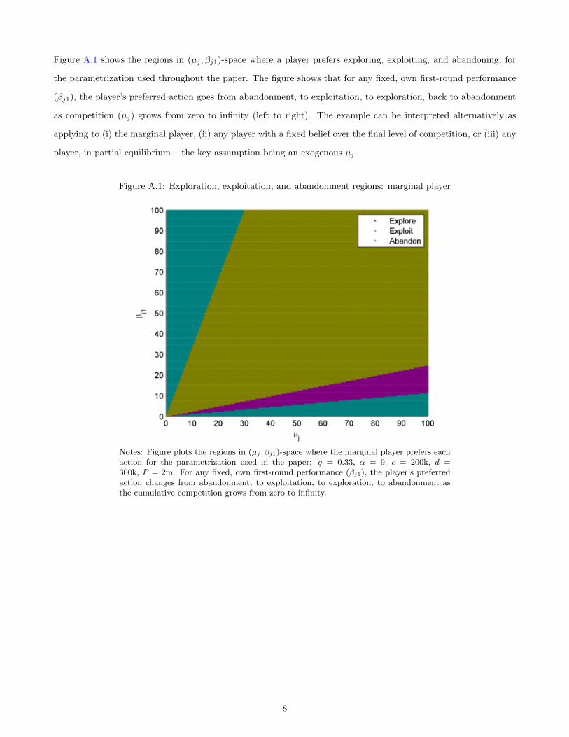
Figure A.1 shows the regions in (µj , βj1)-space where a player prefers exploring, exploiting, and abandoning, for

the parametrization used throughout the paper. The figure shows that for any fixed, own first-round performance

(βj1), the player’s preferred action goes from abandonment, to exploitation, to exploration, back to abandonment

as competition (µj) grows from zero to infinity (left to right). The example can be interpreted alternatively as

applying to (i) the marginal player, (ii) any player with a fixed belief over the final level of competition, or (iii) any

player, in partial equilibrium – the key assumption being an exogenous µj .

Figure A.1: Exploration, exploitation, and abandonment regions: marginal player

Notes: Figure plots the regions in (µj , βj1)-space where the marginal player prefers eachaction for the parametrization used in the paper: q = 0.33, α = 9, c = 200k, d =300k, P = 2m. For any fixed, own first-round performance (βj1), the player’s preferredaction changes from abandonment, to exploitation, to exploration, to abandonment asthe cumulative competition grows from zero to infinity.

8

Figure A.2 performs a similar exercise for a strategic second-to-last player who takes into account the next player’s

best response. Panel (A) shows a simulation where the remaining competitors first-round performance comprises 5

percent of cumulative competition; Panel (B), 10 percent; Panel (C), 20 percent; and Panel (D), 40 percent. The

sequence of preferred actions as competition increases is the same as that in the previous igure, provided that the

remaining competitor is a fraction of the cumulative competition.

Figure A.2: Exploration, exploitation, and abandonment regions: inframarginal player

Panel (A) Panel (B)

Panel (C) Panel (D)

Notes: Figure plots the regions in (µj , βj1)-space where the player with the second-to-last move prefers eachaction for the parametrization used in the paper (q = 0.33, α = 9, c = 200k, d = 300k, P = 2m), takinginto account the next player’s best response. Panel (A) plots the case where the remaining competitor’sfirst-round performance is five percent of the cumulative competition; Panel (B), 10 percent; Panel (C), 20percent; and Panel (D), 40 percent. The incentives are similar to those for marginal or non-strategic playersprovided that the remaining competitor is a fraction of the cumulative competition.

9

B Dataset Construction

Data were collected on all logo design contests with open (i.e., public) bidding that launched the week of

September 3 to 9, 2013, and every three weeks thereafter through the week of November 5 to 11, 2013.

Conditional on open bidding, this sample is effectively randomly drawn. The sample used in the paper is

further restricted to contests with a single, winner-take-all prize and with no mid-contest rule changes such

as prize increases, deadline extensions, and early endings. The sample also excludes one contest that went

dormant and resumed after several weeks, as well as a handful of contests whose sponsors simply stopped

participating and were never heard from again. These restrictions cause 146 contests to be dropped from

the sample. The final dataset includes 122 contests, 4,050 contest-players, and 11,758 designs.

To collect the data, I developed an automated script to scan these contests once an hour for new submissions,

save a copy of each design for analysis, and record their owners’ identity and performance history from a player

profile. I successfully obtained the image files for 96 percent of designs in the final sample. The remaining

designs were entered and withdrawn before they could be observed (recall that players can withdraw designs

they have entered into a contest, though this option is rarely exercised and can be reversed at the request

of a sponsor). All other data were automatically acquired at the conclusion of each contest, once the prize

was awarded or the sponsor exercised its outside option of a refund.

B.1 Variables

The dataset includes information on the characteristics of contests, contest-players, and designs:

• Contest-level variables include: the contest sponsor, features of the project brief (title, description,

sponsor industry, materials to be included in logo), start and end dates, the prize amount (and whether

committed), and the number of players and designs of each rating.

• Contest-player-level variables include: the player’s self-reported country, his/her experience in previous

contests on the platform (number of contests and designs entered, contests won), and that player’s

participation and performance in the given contest.

• Design-level variables include: the design’s owner, its submission time and order of entry, the feedback

it received, the time at which this feedback was given, and whether it was eventually withdrawn. For

designs with images acquired, I calculate originality using the procedures described in the next section.

The majority of the analysis occurs at the design level.

Note that designs are occasionally re-rated: five percent of all rated designs are re-rated an average of 1.2

times each. Of these, 14 percent are given their original rating, and 83 percent are re-rated within 1 star of

10

the original rating. I treat the first rating on each design to be the most informative, objective measure of

quality, since research suggests first instincts tend to be most reliable and ratings revisions are likely made

relative to other designs in the contest rather than an objective benchmark.

B.2 Image Comparison Algorithms

This paper uses two distinct algorithms to calculate pairwise similarity scores. One is a perceptual hash

algorithm, which creates a digital signature (hash) for each image from its lowest frequency content. As

the name implies, a perceptual hash is designed to imitate human perception. The second algorithm is a

difference hash, which creates the hash from pixel intensity gradients.

I implement the perceptual hash algorithm and calculate pairwise similarity scores using a variant of the

procedure described by the Hacker Factor blog.1 This requires six steps:

1. Resize each image to 32x32 pixels and convert to grayscale.

2. Compute the discrete cosine transform (DCT) of each image. The DCT is a widely-used transform

in signal processing that expresses a finite sequence of data points as a linear combination of cosine

functions oscillating at different frequencies. By isolating low frequency content, the DCT reduces a

signal (in this case, an image) to its underlying structure. The DCT is broadly used in digital media

compression, including MP3 and JPEG formats.

3. Retain the upper-left 16x16 DCT coefficients and calculate the average value, excluding first term.

4. Assign 1s to grid cells with above-average DCT coefficients, and 0s elsewhere.

5. Reshape to 256 bit string; this is the image’s digital signature (hash).

6. Compute the Hamming distance between the two hashes and divide by 256.

The similarity score is obtained by subtracting this fraction from one. In a series of sensitivity tests, the

perceptual hash algorithm was found to be strongly invariant to transformations in scale, aspect ratio,

brightness, and contrast, albeit not rotation. As described, the algorithm will perceive two images that

have inverted colors but are otherwise identical to be perfectly dissimilar. I make the algorithm robust to

color inversion by comparing each image against the regular and inverted hash of its counterpart in the pair,

taking the maximum similarity score, and rescaling so that the scores remain in [0,1]. The resulting score is

approximately the absolute value correlation of two images’ content.

1See http://www.hackerfactor.com/blog/archives/432-Looks-Like-It.html.

11

I follow a similar procedure outlined by the same blog2 to implement the difference hash algorithm and

calculate an alternative set of similarity scores for robustness checks:

1. Resize each image to 17x16 pixels and convert to grayscale.

2. Calculate horizontal gradient as the change in pixel intensity from left to right, returning a 16x16 grid

(note: top to bottom is an equally valid alternative)

3. Assign 1s to grid cells with positive gradient, 0s to cells with negative gradient.

4. Reshape to 256 bit string; this is the image’s digital signature (hash).

5. Compute the Hamming distance between the two hashes and divide by 256.

The similarity score is obtained by subtracting this fraction from one. In sensitivity tests, the difference hash

algorithm was found to be highly invariant to transformations in scale and aspect ratio, potentially sensitive

to changes in brightness and contrast, and very sensitive to rotation. I make the algorithm robust to color

inversion using a procedure identical to that described for the perceptual hash.

Though the perceptual and difference hash algorithms are both conceptually and mathematically distinct,

and the resulting similarity scores are only modestly correlated (ρ = 0.38), the empirical results of Section 3

are qualitatively and quantitatively similar under either algorithm. This consistency is reassurance that the

patterns found are not simply an artifact of an arcane image processing algorithm; rather, they appear to

be generated by the visual content of the images themselves.

B.3 Why use algorithms?

There are three advantages to using algorithms over human judges. The first is that the algorithms provide

a consistent, objective measure of similarity, whereas individuals can have significantly different, subjective

perceptions of similarity in practice (Tirilly et al. 2012). This conclusion is supported by a pilot study I

attempted using Amazon Mechanical Turk, in which I asked participants to rate the similarity of pairs of

images they were shown; the results (not provided here) were generally very noisy, except in cases of nearly

identical images, in which case the respondents tended to agree. The second advantage to algorithms over

human judges is that algorithms can be directed to evaluate specific features of an image (in this case, the

low frequency content or pixel intensity gradient), while human judges will see what they choose to see, and

may be attuned to different features in different comparisons. The final advantage of algorithms is more

obvious: they are cheap, taking only seconds to execute a comparison.

2See http://www.hackerfactor.com/blog/archives/529-Kind-of-Like-That.html.

12

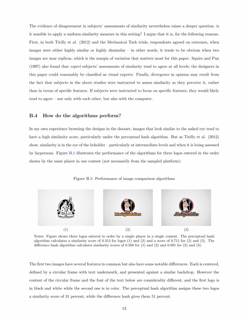
The evidence of disagreement in subjects’ assessments of similarity nevertheless raises a deeper question: is

it sensible to apply a uniform similarity measure in this setting? I argue that it is, for the following reasons.

First, in both Tirilly et al. (2012) and the Mechanical Turk trials, respondents agreed on extremes, when

images were either highly similar or highly dissimilar – in other words, it tends to be obvious when two

images are near replicas, which is the margin of variation that matters most for this paper. Squire and Pun

(1997) also found that expert subjects’ assessments of similarity tend to agree at all levels; the designers in

this paper could reasonably be classified as visual experts. Finally, divergence in opinion may result from

the fact that subjects in the above studies were instructed to assess similarity as they perceive it, rather

than in terms of specific features. If subjects were instructed to focus on specific features, they would likely

tend to agree – not only with each other, but also with the computer.

B.4 How do the algorithms perform?

In my own experience browsing the designs in the dataset, images that look similar to the naked eye tend to

have a high similarity score, particularly under the perceptual hash algorithm. But as Tirilly et al. (2012)

show, similarity is in the eye of the beholder – particularly at intermediate levels and when it is being assessed

by laypersons. Figure B.1 illustrates the performance of the algorithms for three logos entered in the order

shown by the same player in one contest (not necessarily from the sampled platform):

Figure B.1: Performance of image comparison algorithms

(1) (2) (3)

Notes: Figure shows three logos entered in order by a single player in a single contest. The perceptual hashalgorithm calculates a similarity score of 0.313 for logos (1) and (2) and a score of 0.711 for (2) and (3). Thedifference hash algorithm calculates similarity scores of 0.508 for (1) and (2) and 0.891 for (2) and (3).

The first two images have several features in common but also have some notable differences. Each is centered,

defined by a circular frame with text underneath, and presented against a similar backdrop. However the

content of the circular frame and the font of the text below are considerably different, and the first logo is

in black and white while the second one is in color. The perceptual hash algorithm assigns these two logos

a similarity score of 31 percent, while the difference hash gives them 51 percent.

13

In contrast, the second two images appear much more similar. They again have similar layouts, but now they

share the same color assignments and the same content in the frame. Lesser differences remain, primarily

with respect to the font style, but the logos appear broadly similar. The perceptual hash algorithm assigns

these two logos a similarity score of 71 percent; the difference hash, 89 percent.

The algorithms thus pass the gut check in this example, which is not particularly unique: further examples

using better-known brands are provided below. In light of this evidence, and the consistency of the paper’s

results, I believe that these algorithms provide empirically valid measures of experimentation.

Figure B.2: Volkswagen logo in 1937, 1967, 1995, 1999

(1937) (1967) (1995) (1999)

Notes: Figure shows the evolution of Volkswagen logos since 1937. The perceptual hash algorithmcalculates similarity scores of 0.055 for the 1937 and 1967 logos, 0.430 for the 1967 and 1995 logos,and 0.844 for the 1995 and 1999 logos. The difference hash algorithm calculates similarity scores of0.195, 0.539, and 0.953, respectively.

Figure B.3: Microsoft Windows 95, XP, 7, and 8 logos

(Windows 95) (Windows XP) (Windows 7) (Windows 8)

Notes: Figure shows a sequence of Windows logos. The perceptual hash algorithm calculatessimilarity scores of 0.195 for the Windows 95 and XP logos, 0.531 for the Windows XP and 7 logos,and 0.148 for the Windows 7 and 8 logos. The difference hash algorithm calculates similarity scoresof 0.055, 0.563, and 0.117, respectively. The reason why the similarity of the Windows XP and 7logos is not evaluated to be even higher is because the contrast generated by the latter’s spotlightand shadow changes the structure of the image (for example, it changes the intensity gradientcalculated by the difference hash algorithm).

Appendix References:

[1] Tirilly, Pierre, Chunsheng Huang, Wooseob Jeong, Xiangming Mu, Iris Xie, and Jin Zhang. 2012. “Image

Similarity as Assessed by Users: A Quantitative Study.” Proceedings of the American Society for Information

Science and Technology, 49(1), pp. 1-10.

[2] Squire, David and Thierry Pun. 1997. “A Comparison of Human and Machine Assessments of Image

Similarity for the Organization of Image Databases.” Proceedings of the Scandinavian Conference on Image

Analysis, Lappeenranta, Finland.

14

C Contest Characteristics: Evidence from Gross (2015)

To highlight some of the basic features and relationships in these logo design contests, I reproduce a subset

of the results in Gross (2015), which uses a larger sample from the same setting. Table C.1 estimates the

relationship between contest characteristics such as the prize, frequency of feedback, and other characteristics

with key outcomes, and Table C.2 estimates the relationship between a design’s rating and its probability

of being selected. The results are discussed in greater detail in the body of the paper.

Table C.1: Correlations of contest outcomes with their characteristics

(1) (2) (3) (4)Players Designs Designs/Player Awarded

Total Prize Value ($100s) 13.314*** 47.695*** 0.050*** 0.101***(0.713) (2.930) (0.016) (0.027)

Committed Value ($100s) 2.469** 8.674* 0.038(1.205) (4.932) (0.025)

Fraction Rated -7.321*** 15.195*** 1.026*** 1.121***(0.813) (3.098) (0.041) (0.102)

Contest Length 0.537*** 2.109*** 0.013*** 0.021**(0.073) (0.283) (0.004) (0.010)

Words in Desc. (100s) 0.130 3.228*** 0.063*** -0.143***(0.092) (0.449) (0.006) (0.013)

Attached Materials -0.943*** -1.884*** 0.048*** -0.021(0.173) (0.692) (0.013) (0.015)

Prize Committed 1.398 4.539 -0.007(3.559) (14.552) (0.087)

Constant -2.445 -63.730*** 1.916*** 1.085***(2.309) (9.045) (0.072) (0.155)

N 4294 4294 4294 3298R2 0.57 0.54 0.22

Notes: Table shows the estimated effect of contest attributes on overall participation andthe probability that the prize is awarded, using the extended sample of Gross (2015).The final specification is estimated as a probit on contests without a committed prize.*, **, *** represent significance at the 0.1, 0.05, and 0.01 levels, respectively. Monthlyfixed effects included but not shown. Robust SEs in parentheses.

Table C.2: Conditional logit of win-lose outcomes on ratings

Model: Latent design value νijk = γ5 + γ4 + γ3 + γ2 + γ1 + γ∅ + εijk

Fixed effect Est. S.E. t-stat Implied β (eqs. 1-2)Rating==5 1.53 0.07 22.17 4.618Rating==4 -0.96 0.06 -15.35 0.383Rating==3 -3.39 0.08 -40.01 0.034Rating==2 -5.20 0.17 -30.16 0.006Rating==1 -6.02 0.28 -21.82 0.002No rating -3.43 0.06 -55.35 0.032

Notes: Table provides results from a conditional logit estimation of the win-loseoutcome of each design as a function of its rating, using the extended sample ofGross (2015). Outside option is not awarding the prize, with utility normalizedto zero. The results can be used to approximate a player’s probability ofwinning a contest as a function of her ratings. As a measure of fit, the designpredicted by this model as the odds-on favorite wins roughly 50 percent ofcontests. See Gross (2015) for further discussion.

15

Table C.3 below sheds more light on the source of the conditional logit estimates, which are difficult to

interpret directly without a model.3 The table shows a cross-tabulation of contests, by the highest rating

granted (columns) and the rating of the winning design (rows).

Table C.3: Frequency of contests, by highest rating and winning rating

Rating of Highest rating in contestwinner Unrated 1-star 2-star 3-star 4-star 5-star Total

Not awarded 66 4 12 92 202 85 461Unrated 142 5 10 59 347 276 8391-star . . . 3 6 5 142-star . . 3 11 16 8 383-star . . . 43 146 53 2424-star . . . . 836 379 1,2155-star . . . . . 1,485 1,485

Total 208 9 25 208 1,553 2,291 4,294

Notes: Table shows the frequency of contests in Gross (2015) by the highest rating grantedand the rating of the winning design.

Evidence that the samples are comparable

The dataset in Gross (2015) consists of nearly all logo design contests with open bidding completed on the

platform between July 1, 2010 and June 30, 2012, excluding those with zero prizes, multiple prizes, mid-

contest rule changes, or otherwise unusual behavior, and it includes nearly all of the same information as

the sample in this paper – except for the designs themselves. Although this sample comes from a slightly

earlier time period than the one in the present paper (which was collected in the fall of 2013), both cover

periods well after the platform was created and its growth had begun to stabilize.

Table C.4 compares characteristics of contests in the two samples. The contests in the Gross (2015) sample

period are on average slightly longer, offer larger prizes, and attract a bit more participation relative to the

sample of the present paper, but otherwise, the two samples are similar on observables. These differences

are mostly due to the presence of a handful of outlying large contests in the Gross (2015) data. Interestingly,

although the total number of designs is on average higher in the Gross (2015) sample, the number of designs

of each rating is on average the same; the difference in total designs is fully accounted for by an increase in

unrated entries. The most notable difference between the two samples is in the fraction of contests with a

committed prize (23 percent vs. 56 percent). This discrepancy is explained by the fact that prize commitment

only became an option on the platform halfway through the Gross (2015) sample period. Interestingly, the

fraction of contests awarded is nevertheless nearly the same in these two samples.

3I thank Jonah Rockoff for suggesting this table.

16

Table C.4: Comparing Samples: Contest characteristics

Gross (2015) This paperSample size 4,294 122Contest length (days) 9.15 8.52Prize value (US$) 295.22 247.57No. of players 37.28 33.20No. of designs 115.52 96.38

5-star designs 3.41 2.594-star designs 13.84 12.283-star designs 22.16 22.162-star designs 16.04 17.611-star designs 10.94 12.11Unrated designs 49.14 29.62

Number rated 66.38 66.75Fraction rated 0.56 0.64Prize committed 0.23 0.56Prize awarded 0.89 0.85

Tables C.5 and C.6 compare the distribution of ratings and batches in the two samples. The tables demon-

strate that individual behavior is consistent across samples: sponsors assign each rating, and players enter

designs, at roughly the same frequency. The main differences between the two samples are thus isolated to

a handful of the overall contest characteristics highlighted in the previous table.

Table C.5: Comparing Samples: Distribution of ratings

Gross (2015) This paperSample size 285,052 8,1441 star (in percent) 16.48 18.152 stars 24.16 26.393 stars 33.38 33.194 stars 20.84 18.395 stars 5.13 3.88

100.00 100.00

Table C.6: Comparing Samples: Design batches by size of batch

Gross (2015) This paperSample size 335,016 8,0721 design (in percent) 72.46 71.842 designs 17.04 18.623 designs 5.75 5.574 designs 2.50 2.195+ designs 2.25 1.77

100.00 100.00

17

D Robustness Checks (1)

The following tables provide variants of the tables in Section 3 estimating the effects of feedback and com-

petition on experimentation, using the difference hash algorithm instead of the preferred, perceptual hash

algorithm. These estimates serve as robustness checks to the principal empirical results of the paper, demon-

strating that they are not sensitive to the procedure used to calculate similarity scores.

Table D.1 is a robustness check on Table 4; Table D.2, on Table 5; Table D.3, on Table 6; Table D.4, on

Table 7; and Table D.5, on Table 8. The results in these appendix tables are qualitatively and quantitatively

similar to those in the body of the paper.

Table D.1: Similarity to any of player’s previous designs (diff. hash)

(1) (2) (3) (4)Player’s prior best rating==5 0.268*** 0.253*** 0.266*** 0.248***

(0.086) (0.087) (0.086) (0.085)* 1+ competing 5-stars -0.128** -0.141** -0.132** -0.139**

(0.058) (0.056) (0.059) (0.056)* prize value ($100s) -0.037 -0.047* -0.036 -0.049*

(0.026) (0.027) (0.026) (0.026)Player’s prior best rating==4 0.056*** 0.025 0.054*** 0.021

(0.020) (0.021) (0.020) (0.021)Player’s prior best rating==3 0.027 0.011 0.025 0.007

(0.017) (0.017) (0.017) (0.016)Player’s prior best rating==2 -0.004 -0.012 -0.007 -0.017

(0.020) (0.020) (0.020) (0.020)One or more competing 5-stars -0.012 -0.022 -0.012 -0.023

(0.023) (0.024) (0.023) (0.024)Pct. of contest elapsed 0.041 -0.018 0.039 -0.020

(0.029) (0.072) (0.029) (0.073)Constant 0.455*** 0.454*** 0.456*** 0.449***

(0.141) (0.160) (0.141) (0.161)N 5075 5075 5075 5075R2 0.48 0.48 0.48 0.48Controls No Yes No YesContest FEs Yes Yes Yes YesPlayer FEs Yes Yes Yes YesForthcoming ratings No No Yes Yes

Notes: Table shows the effects of feedback on originality. Observations are designs. Depen-dent variable is a continuous measure of a design’s maximal similarity to previous entries inthe same contest by the same player, taking values in [0,1], where a value of 1 indicates thedesign is identical to another. The mean value of this variable is 0.58 (s.d. 0.28). Columns(2) and (4) control for days remaining and number of previous designs by the player and hercompetitors. Columns (3) and (4) additionally control for the best forthcoming rating on theplayer’s not-yet-rated designs. Similarity scores in this table are calculated using a differencehash algorithm. Preceding designs/ratings are defined to be those entered/provided at least60 minutes prior to the given design. *, **, *** represent significance at the 0.1, 0.05, and0.01 levels, respectively. Standard errors clustered by player in parentheses.

18

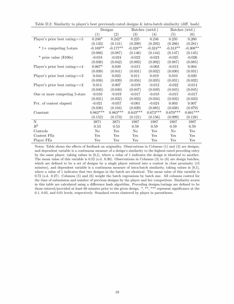
Table D.2: Similarity to player’s best previously-rated designs & intra-batch similarity (diff. hash)

Designs Batches (uwtd.) Batches (wtd.)(1) (2) (3) (4) (5) (6)

Player’s prior best rating==5 0.246* 0.242* 0.225 0.246 0.235 0.260(0.133) (0.141) (0.299) (0.293) (0.286) (0.281)

* 1+ competing 5-stars -0.169** -0.177** -0.328** -0.324** -0.313** -0.308**(0.086) (0.087) (0.146) (0.144) (0.147) (0.145)

* prize value ($100s) -0.018 -0.024 -0.022 -0.023 -0.025 -0.026(0.038) (0.042) (0.093) (0.092) (0.087) (0.085)

Player’s prior best rating==4 0.067* 0.049 -0.015 -0.003 -0.013 0.004(0.039) (0.041) (0.031) (0.032) (0.030) (0.031)

Player’s prior best rating==3 0.044 0.033 0.011 0.019 0.010 0.020(0.038) (0.039) (0.034) (0.035) (0.031) (0.032)

Player’s prior best rating==2 0.014 0.007 -0.019 -0.012 -0.022 -0.014(0.040) (0.040) (0.047) (0.049) (0.045) (0.045)

One or more competing 5-stars -0.010 -0.019 -0.017 -0.018 -0.015 -0.017(0.031) (0.032) (0.033) (0.034) (0.032) (0.033)

Pct. of contest elapsed -0.021 -0.057 -0.001 -0.024 0.003 0.007(0.038) (0.104) (0.039) (0.085) (0.038) (0.079)

Constant 0.862*** 0.863*** 0.643*** 0.673*** 0.670*** 0.661***(0.152) (0.173) (0.121) (0.156) (0.099) (0.128)

N 3871 3871 1987 1987 1987 1987R2 0.53 0.53 0.59 0.59 0.59 0.59Controls No Yes No Yes No YesContest FEs Yes Yes Yes Yes Yes YesPlayer FEs Yes Yes Yes Yes Yes Yes

Notes: Table shows the effects of feedback on originality. Observations in Columns (1) and (2) are designs,and dependent variable is a continuous measure of a design’s similarity to the highest-rated preceding entryby the same player, taking values in [0,1], where a value of 1 indicates the design is identical to another.The mean value of this variable is 0.52 (s.d. 0.30). Observations in Columns (3) to (6) are design batches,which are defined to be a set of designs by a single player entered into a contest in close proximity (15minutes), and dependent variable is a continuous measure of intra-batch similarity, taking values in [0,1],where a value of 1 indicates that two designs in the batch are identical. The mean value of this variable is0.72 (s.d. 0.27). Columns (5) and (6) weight the batch regressions by batch size. All columns control forthe time of submission and number of previous designs by the player and her competitors. Similarity scoresin this table are calculated using a difference hash algorithm. Preceding designs/ratings are defined to bethose entered/provided at least 60 minutes prior to the given design. *, **, *** represent significance at the0.1, 0.05, and 0.01 levels, respectively. Standard errors clustered by player in parentheses.

19

Table D.3: Change in similarity to player’s best previously-rated designs (diff. hash)

(1) (2) (3) (4) (5) (6)∆(Player’s best rating==5) 0.658*** 0.679*** 0.688** 0.659*** 0.693*** 0.693***

(0.218) (0.256) (0.268) (0.217) (0.256) (0.267)* 1+ competing 5-stars -0.349** -0.375* -0.364* -0.350** -0.379* -0.368*

(0.175) (0.207) (0.218) (0.174) (0.206) (0.218)* prize value ($100s) -0.048 -0.059 -0.062 -0.048 -0.063 -0.064

(0.046) (0.055) (0.057) (0.046) (0.055) (0.057)∆(Player’s best rating==4) 0.262*** 0.236*** 0.232*** 0.262*** 0.237*** 0.232***

(0.070) (0.081) (0.086) (0.070) (0.081) (0.086)∆(Player’s best rating==3) 0.192*** 0.170** 0.162** 0.192*** 0.169** 0.162**

(0.062) (0.073) (0.077) (0.063) (0.073) (0.077)∆(Player’s best rating==2) 0.133** 0.110 0.104 0.131** 0.110 0.104

(0.058) (0.068) (0.071) (0.058) (0.067) (0.071)One or more competing 5-stars -0.002 0.002 -0.001 0.001 0.000 -0.001

(0.017) (0.017) (0.028) (0.018) (0.016) (0.029)Pct. of contest elapsed -0.007 -0.011 -0.014 -0.067 -0.073 -0.104

(0.020) (0.029) (0.036) (0.062) (0.064) (0.110)Constant -0.009 -0.008 -0.238*** 0.058 0.038 -0.169**

(0.010) (0.017) (0.036) (0.050) (0.047) (0.072)N 2694 2694 2694 2694 2694 2694R2 0.04 0.10 0.13 0.04 0.10 0.13Controls No No No Yes Yes YesContest FEs Yes No Yes Yes No YesPlayer FEs No Yes Yes No Yes Yes

Notes: Table shows the effects of feedback on originality. Observations are designs. Dependent variable isa continuous measure of the change in designs’ similarity to the highest-rated preceding entry by the sameplayer, taking values in [-1,1], where a value of 0 indicates that the player’s current design is as similar toher best preceding design as was her previous design, and a value of 1 indicates that the player transitionedfully from experimenting to copying (and a value of -1, the converse). The mean value of this variable is-0.01 (s.d. 0.25). Columns (4) to (6) control for days remaining and number of previous designs by the playerand competitors. Similarity scores in this table are calculated using a difference hash algorithm. Precedingdesigns/ratings are defined to be those entered/provided at least 60 minutes prior to the given design. *, **,*** represent significance at the 0.1, 0.05, and 0.01 levels, respectively. Standard errors clustered by playerin parentheses.

20

Table D.4: Similarity to player’s best not-yet-rated designs (placebo test; using diff. hash)

Similarity to forthcoming Residual(1) (2) (3) (4)

Player’s best forthcoming rating==5 0.203 0.069 0.022 0.060(0.241) (0.116) (0.127) (0.119)

* 1+ competing 5-stars -0.040 -0.024 0.000 -0.023(0.145) (0.073) (0.080) (0.079)

* prize value ($100s) -0.064 -0.009 -0.001 -0.006(0.042) (0.028) (0.032) (0.029)

Player’s best forthcoming rating==4 0.023 0.051 0.059 0.045(0.074) (0.066) (0.064) (0.067)

Player’s best forthcoming rating==3 0.043 0.069 0.069 0.055(0.050) (0.055) (0.055) (0.053)

Player’s best forthcoming rating==2 0.031 0.025 0.026 0.025(0.048) (0.051) (0.051) (0.049)

One or more competing 5-stars -0.077 -0.089 -0.087 -0.085(0.076) (0.115) (0.119) (0.124)

Pct. of contest elapsed -0.210 0.033 0.093 0.023(0.261) (0.442) (0.422) (0.469)

Constant 0.826** 0.491 0.515 0.060(0.357) (0.412) (0.472) (0.507)

N 1147 577 577 577R2 0.69 0.87 0.88 0.69Controls Yes Yes Yes YesContest FEs Yes Yes Yes YesPlayer FEs Yes Yes Yes Yes

Notes: Table provides a placebo test of the effects of future feedback on originality. Obser-vations are designs. Dependent variable in Columns (1) to (3) is a continuous measure of adesign’s similarity to the best design that the player has previously entered that has yet tobut will eventually be rated, taking values in [0,1], where a value of 1 indicates that the twodesigns are identical. The mean value of this variable is 0.50 (s.d. 0.29). Under the identify-ing assumption that future feedback is unpredictable, current choices should be unrelated toforthcoming ratings. Note that a given design’s similarity to an earlier, unrated design canbe incidental if they are both tweaks on a rated third design. To account for this possibility,Column (2) controls for the given and unrated designs’ similarity to the best previously-rateddesign. Column (3) allows these controls to vary with the highest rating previously received.Dependent variable in Column (4) is the residual from a regression of the dependent variablein the previous columns on these controls. These residuals will be the subset of a given design’ssimilarity to the unrated design that is not explained by jointly-occurring similarity to a thirddesign. All columns control for days remaining and number of previous designs by the playerand her competitors. Similarity scores in this table are calculated using a difference hash algo-rithm. Preceding designs/ratings are defined to be those entered/provided at least 60 minutesprior to the given design. *, **, *** represent significance at the 0.1, 0.05, and 0.01 levels,respectively. Standard errors clustered by player in parentheses.

21

Table D.5: Similarity and change in similarity to competitors’ best previously-rated designs (diff. hash)

(1) (2) (3) (4)Competitors’ best==5 -0.199*** -0.127*** ∆(Competitors’ best==5) -0.06 -0.058

-0.046 -0.048 -0.11 (0.110)* 1+ own 5-stars -0.016 -0.022 * 1+ own 5-stars -0.006 -0.011

-0.034 -0.035 -0.066 (0.066)* prize value ($100s) 0.029*** 0.005 * prize value ($100s) 0.001 -0.001

-0.009 -0.009 -0.02 (0.020)Competitors’ best==4 0.018 0.033 ∆(Competitors’ best==4) 0.07 0.070

-0.035 -0.035 -0.084 (0.085)Competitors’ best==3 0.032 0.045 ∆(Competitors’ best==3) 0.069 0.070

-0.034 -0.034 -0.084 (0.084)Competitors’ best==2 -0.057 -0.052 ∆(Competitors’ best==2) 0.014 0.016

-0.04 -0.04 -0.085 (0.085)One or more own 5-stars -0.005 0.005 One or more own 5-stars 0.015 0.020

-0.027 -0.03 -0.012 (0.013)Pct. of contest elapsed 0.133*** 0.138*** Pct. of contest elapsed -0.004 0.021

-0.014 -0.04 -0.01 (0.027)Constant 0.431*** 0.045 Constant 0.04 0.017

-0.103 -0.101 -0.066 (0.071)N 9709 9709 N 6065 6065R2 0.54 0.54 R2 0.14 0.15Controls No Yes Controls No YesContest FEs Yes Yes Contest FEs Yes YesPlayer FEs Yes Yes Player FEs Yes Yes

Notes: Table provides a test of players’ ability to discern the quality of, and then imitate, competing designs.Observations are designs. Dependent variable in Columns (1) and (2) is a continuous measure of the design’ssimilarity to the highest-rated preceding entries by other players, taking values in [0,1], where a value of 1indicates that the design is identical to another. The mean value in the sample is 0.33 (s.d. 0.21). Dependentvariable in Columns (3) and (4) is a continuous measure of the change in designs’ similarity to the highest-rated preceding entries by other players, taking values in [-1,1], where a value of 0 indicates that the player’scurrent design is equally similar to the best competing design as was her previous design, and a value of 1indicates that the player transitioned fully from experimenting to copying (and a value of -1, the converse).The mean value of this variable is 0.00 (s.d. 0.15). In general, players are provided only the distribution ofratings on competing designs; ratings of specific competing designs are not observed. Results in this tabletest whether players can nevertheless identify and imitate leading competition. Columns (2) and (4) controlfor days remaining and number of previous designs by the player and her competitors. Similarity scoresin this table are calculated using a difference hash algorithm. Preceding designs/ratings are defined to bethose entered/provided at least 60 minutes prior to the given design. *, **, *** represent significance at the0.1, 0.05, and 0.01 levels, respectively. Standard errors clustered by player in parentheses.

22

E Robustness Checks (2)

In additional robustness checks, I show that competition has a constant effect on high-performing players’

tendency to experiment. Tables E.1 to E.3 demonstrate this result with the perceptual hash similarity

measures, and Tables E.4 to E.6 do so with the difference hash measures. In all cases, I estimate differential

effects for one vs. multiple top-rated, competing designs and find no differential effect.

Table E.1: Similarity to any of player’s previous designs (p. hash)

(1) (2) (3) (4)Player’s prior best rating==5 0.287*** 0.280*** 0.288*** 0.278***

(0.086) (0.088) (0.085) (0.088)* 1+ competing 5-stars -0.157* -0.158* -0.155* -0.153*

(0.093) (0.089) (0.094) (0.089)* 2+ competing 5-stars 0.060 0.052 0.063 0.056

(0.111) (0.098) (0.110) (0.096)* prize value ($100s) -0.012 -0.022 -0.014 -0.026

(0.028) (0.028) (0.028) (0.028)Player’s prior best rating==4 0.099*** 0.076*** 0.099*** 0.074***

(0.017) (0.017) (0.017) (0.018)Player’s prior best rating==3 0.039*** 0.028* 0.039*** 0.026*

(0.014) (0.014) (0.014) (0.014)Player’s prior best rating==2 -0.004 -0.009 -0.003 -0.011

(0.020) (0.020) (0.020) (0.020)One or more competing 5-stars 0.006 0.005 0.006 0.005

(0.032) (0.032) (0.032) (0.032)Two or more competing 5-stars -0.024 -0.035 -0.024 -0.035

(0.035) (0.037) (0.035) (0.037)Pct. of contest elapsed 0.039 -0.095 0.040 -0.094

(0.028) (0.073) (0.028) (0.073)Constant 0.292 0.408** 0.290 0.400**

(0.180) (0.196) (0.180) (0.197)N 5075 5075 5075 5075R2 0.47 0.47 0.47 0.47Controls No Yes No YesContest FEs Yes Yes Yes YesPlayer FEs Yes Yes Yes YesForthcoming ratings No No Yes Yes

Notes: Table shows the effects of feedback on originality. Observations are designs. Depen-dent variable is a continuous measure of a design’s maximal similarity to previous entries inthe same contest by the same player, taking values in [0,1], where a value of 1 indicates thedesign is identical to another. The mean value of this variable is 0.32 (s.d. 0.27). Columns(2) and (4) control for days remaining and number of previous designs by the player and hercompetitors. Columns (3) and (4) additionally control for the best forthcoming rating on theplayer’s not-yet-rated designs. Similarity scores in this table are calculated using a percep-tual hash algorithm. Preceding designs/ratings are defined to be those entered/provided atleast 60 minutes prior to the given design. *, **, *** represent significance at the 0.1, 0.05,and 0.01 levels, respectively. Standard errors clustered by player in parentheses.

23

Table E.2: Similarity to player’s best previously-rated designs & intra-batch similarity (p. hash)

Designs Batches (uwtd.) Batches (wtd.)(1) (2) (3) (4) (5) (6)

Player’s prior best rating==5 0.358*** 0.362*** 0.213 0.240 0.245 0.285(0.098) (0.103) (0.312) (0.307) (0.302) (0.294)

* 1+ competing 5-stars -0.225** -0.226** -0.437** -0.433** -0.475** -0.469**(0.093) (0.093) (0.217) (0.214) (0.203) (0.200)

* 2+ competing 5-stars 0.025 0.023 0.180 0.177 0.237 0.238(0.094) (0.092) (0.236) (0.232) (0.223) (0.218)

* prize value ($100s) -0.014 -0.018 0.020 0.015 0.013 0.009(0.031) (0.033) (0.099) (0.099) (0.095) (0.093)

Player’s prior best rating==4 0.122*** 0.116*** 0.055* 0.066* 0.065** 0.086**(0.031) (0.032) (0.032) (0.037) (0.032) (0.038)

Player’s prior best rating==3 0.061** 0.056** 0.056 0.062* 0.052 0.065*(0.028) (0.028) (0.035) (0.037) (0.035) (0.037)

Player’s prior best rating==2 0.026 0.024 0.023 0.029 0.009 0.020(0.030) (0.030) (0.049) (0.050) (0.047) (0.047)

One or more competing 5-stars 0.002 0.002 0.083 0.086 0.076 0.078(0.037) (0.037) (0.063) (0.063) (0.063) (0.063)

Two or more competing 5-stars 0.004 0.000 -0.094 -0.100 -0.080 -0.086(0.042) (0.044) (0.072) (0.076) (0.074) (0.076)

Pct. of contest elapsed -0.019 -0.103 -0.016 -0.102 -0.005 -0.064(0.034) (0.084) (0.049) (0.115) (0.050) (0.112)

Constant 0.422** 0.487*** 0.392*** 0.504*** 0.385*** 0.457***(0.168) (0.187) (0.066) (0.149) (0.061) (0.148)

N 3871 3871 1987 1987 1987 1987R2 0.53 0.53 0.58 0.58 0.58 0.58Controls No Yes No Yes No YesContest FEs Yes Yes Yes Yes Yes YesPlayer FEs Yes Yes Yes Yes Yes Yes

Notes: Table shows the effects of feedback on originality. Observations in Columns (1) and (2) are designs,and dependent variable is a continuous measure of a design’s similarity to the highest-rated preceding entryby the same player, taking values in [0,1], where a value of 1 indicates the design is identical to another.The mean value of this variable is 0.28 (s.d. 0.27). Observations in Columns (3) to (6) are design batches,which are defined to be a set of designs by a single player entered into a contest in close proximity (15minutes), and dependent variable is a continuous measure of intra-batch similarity, taking values in [0,1],where a value of 1 indicates that two designs in the batch are identical. The mean value of this variable is0.48 (s.d. 0.32). Columns (5) and (6) weight the batch regressions by batch size. All columns control forthe time of submission and number of previous designs by the player and her competitors. Similarity scoresin this table are calculated using a perceptual hash algorithm. Preceding designs/ratings are defined to bethose entered/provided at least 60 minutes prior to the given design. *, **, *** represent significance at the0.1, 0.05, and 0.01 levels, respectively. Standard errors clustered by player in parentheses.

24

Table E.3: Change in similarity to player’s best previously-rated designs (p. hash)

(1) (2) (3) (4) (5) (6)∆(Player’s best rating==5) 0.879*** 0.934*** 0.921*** 0.886*** 0.934*** 0.928***

(0.166) (0.194) (0.200) (0.167) (0.193) (0.200)* 1+ competing 5-stars -0.487*** -0.534*** -0.504*** -0.489*** -0.532*** -0.505***

(0.133) (0.150) (0.160) (0.134) (0.150) (0.161)* 2+ competing 5-stars 0.099 0.162 0.108 0.099 0.158 0.107

(0.111) (0.123) (0.127) (0.112) (0.123) (0.127)* prize value ($100s) -0.093** -0.115*** -0.108** -0.095** -0.114** -0.110**

(0.037) (0.044) (0.044) (0.038) (0.044) (0.045)∆(Player’s best rating==4) 0.285*** 0.274*** 0.281*** 0.287*** 0.276*** 0.284***

(0.065) (0.071) (0.077) (0.065) (0.071) (0.077)∆(Player’s best rating==3) 0.154*** 0.141** 0.141** 0.154*** 0.142** 0.142**

(0.057) (0.063) (0.067) (0.057) (0.063) (0.067)∆(Player’s best rating==2) 0.085* 0.069 0.064 0.084* 0.069 0.063

(0.046) (0.052) (0.056) (0.046) (0.052) (0.056)One or more competing 5-stars 0.002 -0.018 -0.014 0.003 -0.019 -0.013

(0.026) (0.031) (0.044) (0.026) (0.032) (0.043)Two or more competing 5-stars -0.006 0.021 0.031 -0.006 0.022 0.029

(0.025) (0.032) (0.041) (0.026) (0.034) (0.043)Pct. of contest elapsed 0.009 0.014 -0.003 -0.036 0.008 -0.050

(0.018) (0.023) (0.029) (0.043) (0.048) (0.074)Constant -0.017* -0.021 0.029 0.024 -0.014 0.058

(0.010) (0.014) (0.061) (0.040) (0.037) (0.078)N 2694 2694 2694 2694 2694 2694R2 0.05 0.11 0.14 0.05 0.11 0.14Controls No No No Yes Yes YesContest FEs Yes No Yes Yes No YesPlayer FEs No Yes Yes No Yes Yes

Notes: Table shows the effects of feedback on originality. Observations are designs. Dependent variable is acontinuous measure of the change in designs’ similarity to the highest-rated preceding entry by the same player,taking values in [-1,1], where a value of 0 indicates that the player’s current design is as similar to her bestpreceding design as was her previous design, and a value of 1 indicates that the player transitioned fully fromexperimenting to copying (and a value of -1, the converse). The mean value of this variable is 0.00 (s.d. 0.23).Columns (4) to (6) control for days remaining and number of previous designs by the player and competitors.Similarity scores in this table are calculated using a perceptual hash algorithm. Preceding designs/ratings aredefined to be those entered/provided at least 60 minutes prior to the given design. *, **, *** represent significanceat the 0.1, 0.05, and 0.01 levels, respectively. Standard errors clustered by player in parentheses.

25

Table E.4: Similarity to any of player’s previous designs (d. hash)

(1) (2) (3) (4)Player’s prior best rating==5 0.267*** 0.250*** 0.266*** 0.245***

(0.087) (0.087) (0.086) (0.085)* 1+ competing 5-stars -0.103 -0.110 -0.105 -0.108

(0.086) (0.080) (0.088) (0.080)* 2+ competing 5-stars -0.033 -0.039 -0.036 -0.040

(0.094) (0.080) (0.095) (0.080)* prize value ($100s) -0.036 -0.046* -0.036 -0.048*

(0.026) (0.027) (0.026) (0.026)Player’s prior best rating==4 0.058*** 0.027 0.056*** 0.023

(0.020) (0.021) (0.020) (0.021)Player’s prior best rating==3 0.028* 0.013 0.026 0.008

(0.017) (0.017) (0.017) (0.017)Player’s prior best rating==2 -0.004 -0.012 -0.007 -0.017

(0.020) (0.020) (0.020) (0.020)One or more competing 5-stars -0.043 -0.044 -0.043 -0.045

(0.037) (0.038) (0.037) (0.038)Two or more competing 5-stars 0.049 0.036 0.048 0.035

(0.037) (0.040) (0.037) (0.040)Pct. of contest elapsed 0.035 -0.020 0.034 -0.022

(0.028) (0.073) (0.028) (0.073)Constant 0.461*** 0.460*** 0.461*** 0.454***

(0.141) (0.160) (0.141) (0.161)N 5075 5075 5075 5075R2 0.48 0.48 0.48 0.48Controls No Yes No YesContest FEs Yes Yes Yes YesPlayer FEs Yes Yes Yes YesForthcoming ratings No No Yes Yes

Notes: Table shows the effects of feedback on originality. Observations are designs. Depen-dent variable is a continuous measure of a design’s maximal similarity to previous entries inthe same contest by the same player, taking values in [0,1], where a value of 1 indicates thedesign is identical to another. The mean value of this variable is 0.58 (s.d. 0.28). Columns(2) and (4) control for days remaining and number of previous designs by the player and hercompetitors. Columns (3) and (4) additionally control for the best forthcoming rating on theplayer’s not-yet-rated designs. Similarity scores in this table are calculated using a differencehash algorithm. Preceding designs/ratings are defined to be those entered/provided at least60 minutes prior to the given design. *, **, *** represent significance at the 0.1, 0.05, and0.01 levels, respectively. Standard errors clustered by player in parentheses.

26

Table E.5: Similarity to player’s best previously-rated designs & intra-batch similarity (d. hash)

Designs Batches (uwtd.) Batches (wtd.)(1) (2) (3) (4) (5) (6)

Player’s prior best rating==5 0.242* 0.234* 0.239 0.271 0.252 0.285(0.134) (0.141) (0.317) (0.312) (0.300) (0.295)

* 1+ competing 5-stars -0.144 -0.149 -0.329** -0.328** -0.328** -0.327**(0.140) (0.138) (0.144) (0.142) (0.132) (0.131)

* 2+ competing 5-stars -0.033 -0.036 0.007 0.009 0.025 0.030(0.143) (0.134) (0.189) (0.186) (0.173) (0.172)

* prize value ($100s) -0.017 -0.022 -0.026 -0.031 -0.030 -0.033(0.039) (0.042) (0.100) (0.099) (0.092) (0.090)

Player’s prior best rating==4 0.068* 0.050 -0.015 -0.002 -0.012 0.004(0.039) (0.041) (0.031) (0.032) (0.030) (0.031)

Player’s prior best rating==3 0.044 0.033 0.012 0.019 0.011 0.020(0.038) (0.039) (0.034) (0.035) (0.031) (0.032)

Player’s prior best rating==2 0.013 0.006 -0.018 -0.011 -0.020 -0.012(0.040) (0.040) (0.047) (0.048) (0.044) (0.045)

One or more competing 5-stars -0.048 -0.050 0.037 0.038 0.030 0.030(0.045) (0.045) (0.042) (0.042) (0.038) (0.038)

Two or more competing 5-stars 0.059 0.052 -0.089* -0.096* -0.076 -0.082(0.049) (0.051) (0.051) (0.055) (0.048) (0.051)

Pct. of contest elapsed -0.030 -0.062 0.006 -0.037 0.008 -0.007(0.037) (0.105) (0.040) (0.085) (0.039) (0.080)

Constant 0.866*** 0.870*** 0.636*** 0.677*** 0.665*** 0.666***(0.152) (0.174) (0.120) (0.156) (0.098) (0.128)

N 3871 3871 1987 1987 1987 1987R2 0.53 0.54 0.59 0.59 0.59 0.59Controls No Yes No Yes No YesContest FEs Yes Yes Yes Yes Yes YesPlayer FEs Yes Yes Yes Yes Yes Yes

Notes: Table shows the effects of feedback on originality. Observations in Columns (1) and (2) are designs,and dependent variable is a continuous measure of a design’s similarity to the highest-rated preceding entryby the same player, taking values in [0,1], where a value of 1 indicates the design is identical to another.The mean value of this variable is 0.52 (s.d. 0.30). Observations in Columns (3) to (6) are design batches,which are defined to be a set of designs by a single player entered into a contest in close proximity (15minutes), and dependent variable is a continuous measure of intra-batch similarity, taking values in [0,1],where a value of 1 indicates that two designs in the batch are identical. The mean value of this variable is0.72 (s.d. 0.27). Columns (5) and (6) weight the batch regressions by batch size. All columns control forthe time of submission and number of previous designs by the player and her competitors. Similarity scoresin this table are calculated using a difference hash algorithm. Preceding designs/ratings are defined to bethose entered/provided at least 60 minutes prior to the given design. *, **, *** represent significance at the0.1, 0.05, and 0.01 levels, respectively. Standard errors clustered by player in parentheses.

27

Table E.6: Change in similarity to player’s best previously-rated designs (d. hash)

(1) (2) (3) (4) (5) (6)∆(Player’s best rating==5) 0.657*** 0.684*** 0.695*** 0.657*** 0.695*** 0.695***

(0.218) (0.253) (0.265) (0.217) (0.253) (0.264)* 1+ competing 5-stars -0.401* -0.452* -0.428* -0.400* -0.456* -0.429*

(0.211) (0.236) (0.255) (0.211) (0.236) (0.256)* 2+ competing 5-stars 0.070 0.108 0.090 0.068 0.109 0.088

(0.154) (0.167) (0.184) (0.155) (0.167) (0.185)* prize value ($100s) -0.047 -0.059 -0.064 -0.047 -0.062 -0.063

(0.046) (0.053) (0.055) (0.045) (0.053) (0.055)∆(Player’s best rating==4) 0.264*** 0.240*** 0.236*** 0.264*** 0.241*** 0.237***

(0.070) (0.081) (0.086) (0.070) (0.081) (0.085)∆(Player’s best rating==3) 0.195*** 0.174** 0.166** 0.194*** 0.173** 0.166**

(0.063) (0.073) (0.077) (0.063) (0.074) (0.077)∆(Player’s best rating==2) 0.135** 0.115* 0.108 0.133** 0.114* 0.108

(0.058) (0.068) (0.071) (0.058) (0.068) (0.071)One or more competing 5-stars -0.011 -0.018 -0.028 -0.008 -0.018 -0.026

(0.030) (0.035) (0.049) (0.029) (0.036) (0.048)Two or more competing 5-stars 0.012 0.029 0.044 0.015 0.026 0.046

(0.027) (0.037) (0.046) (0.028) (0.038) (0.048)Pct. of contest elapsed -0.009 -0.013 -0.023 -0.067 -0.072 -0.107

(0.019) (0.028) (0.034) (0.062) (0.065) (0.110)Constant -0.008 -0.007 -0.238*** 0.059 0.040 -0.171**

(0.010) (0.016) (0.036) (0.049) (0.046) (0.073)N 2694 2694 2694 2694 2694 2694R2 0.04 0.10 0.13 0.04 0.10 0.13Controls No No No Yes Yes YesContest FEs Yes No Yes Yes No YesPlayer FEs No Yes Yes No Yes Yes

Notes: Table shows the effects of feedback on originality. Observations are designs. Dependent variable isa continuous measure of the change in designs’ similarity to the highest-rated preceding entry by the sameplayer, taking values in [-1,1], where a value of 0 indicates that the player’s current design is as similar toher best preceding design as was her previous design, and a value of 1 indicates that the player transitionedfully from experimenting to copying (and a value of -1, the converse). The mean value of this variable is-0.01 (s.d. 0.25). Columns (4) to (6) control for days remaining and number of previous designs by the playerand competitors. Similarity scores in this table are calculated using a difference hash algorithm. Precedingdesigns/ratings are defined to be those entered/provided at least 60 minutes prior to the given design. *, **,*** represent significance at the 0.1, 0.05, and 0.01 levels, respectively. Standard errors clustered by playerin parentheses.

28

F Robustness Checks (3)

The basic fact documented in this paper is the differential tendency for high-performing agents to try new

ideas in the absence versus presence of other high-quality competition. Though the body of the paper focuses

on variation in 5-star ratings, a natural question to ask is whether the same patterns arise for players with

4-star ratings, particularly when that is the highest rating in the contest. In other words: does heart of the

matter have to do with having a 5-star rating, or having the best rating?

Table F.1 explores this question. The table runs regressions similar to those in Table 4, restricted to

observations where there are not yet any 5-star designs in the same contest. The specifications regress the

maximal similarity of the given design to previous entries by the same player on indicators for the player’s

highest rating, interacting the 4-star indicator with 4-star competition. Since the importance of the 4-star

ratings grows towards the end of a contest, as it becomes clear that no higher ratings will be granted, the

table breaks the results out for all submissions (Cols. 1 and 4), submissions in the 2nd half of a contest

(Cols. 2 and 5), and submissions in the 4th quarter (Cols. 3 and 6). The latter three columns in the table

add controls for a player’s highest forthcoming rating, as in the body of the paper.

The evidence suggests the results are general to 4-on-4 competition. In Columns (1) to (3), players whose

highest rating is 4-stars enter designs that are significantly more similar to their previous work than those with

lower ratings, but these effects are reversed by 4-star competition, with both effects growing in magnitude

over the course of a contest – though by the final quarter of a contest, reduced cell sizes cause the standard

errors to rise, such that the estimates become marginally significant or not statistically different from zero.

The results with controls, in the latter three columns, are identical in magnitude and statistical significance.

Table F.2 repeats the exercise using the difference hash algorithm.

29

Table F.1: Similarity to any of player’s previous designs: 4-vs-4 (p. hash)

(1) (2) (3) (4) (5) (6)Player’s prior best rating==4 0.185*** 0.382** 0.564* 0.184*** 0.391** 0.516*

(0.069) (0.190) (0.299) (0.069) (0.196) (0.283)* 1+ competing 4-stars -0.121** -0.323* -0.315 -0.122** -0.325* -0.280

(0.051) (0.181) (0.248) (0.051) (0.185) (0.226)* prize value ($100s) -0.011 -0.006 -0.045 -0.012 -0.010 -0.039

(0.020) (0.033) (0.097) (0.020) (0.033) (0.092)Player’s prior best rating==3 0.006 0.042 -0.029 0.004 0.043 -0.035

(0.023) (0.041) (0.088) (0.024) (0.041) (0.090)Player’s prior best rating==2 -0.016 -0.046 0.040 -0.017 -0.042 0.050

(0.032) (0.057) (0.097) (0.032) (0.055) (0.098)One or more competing 4-stars 0.060** 0.076 0.091 0.059** 0.071 0.098

(0.028) (0.092) (0.169) (0.029) (0.084) (0.152)Pct. of contest elapsed -0.091 -0.638** 0.828 -0.088 -0.631** 0.750

(0.119) (0.274) (0.755) (0.121) (0.271) (0.756)Constant 0.457** 0.948*** -0.956 0.448** 0.900*** -0.410

(0.209) (0.317) (0.742) (0.209) (0.309) (0.905)N 2926 1557 879 2926 1557 879R2 0.52 0.60 0.67 0.52 0.60 0.68Controls Yes Yes Yes Yes Yes YesContest FEs Yes Yes Yes Yes Yes YesPlayer FEs Yes Yes Yes Yes Yes YesForthcoming No No No Yes Yes YesRestriction All 2nd half 4th qtr All 2nd half 4th qtr

Notes: Table shows the effects of 4-star feedback and competition on originality when no player has a 5-starrating. Observations are designs. Dependent variable is a continuous measure of a design’s maximal similarityto previous entries in the same contest by the same player, taking values in [0,1], where a value of 1 indicatesthe design is identical to another. All columns include contest and player fixed effects and control for thetime of submission and number of previous designs by the player and her competitors. Columns (4) to (6)additionally control for the best forthcoming rating on the player’s not-yet-rated designs. The second andthird columns in each block restrict the sample to submissions in the second half or fourth quater of a contest,when the absence of 5-star ratings may be more meaningful and is increasingly likely to be final. Similarityscores in this table are calculated using a perceptual hash algorithm. *, **, *** represent significance at the0.1, 0.05, and 0.01 levels, respectively. Standard errors clustered by player in parentheses.

30

Table F.2: Similarity to any of player’s previous designs: 4-vs-4 (d. hash)

(1) (2) (3) (4) (5) (6)Player’s prior best rating==4 0.087 0.221* 0.745*** 0.084 0.238** 0.715***

(0.068) (0.122) (0.253) (0.068) (0.120) (0.238)* 1+ competing 4-stars -0.105** -0.190** -0.304 -0.107** -0.201** -0.295

(0.047) (0.084) (0.201) (0.047) (0.079) (0.186)* prize value ($100s) 0.006 -0.007 -0.162* 0.006 -0.012 -0.152*

(0.020) (0.037) (0.084) (0.020) (0.036) (0.080)Player’s prior best rating==3 -0.014 -0.009 -0.048 -0.020 -0.010 -0.047

(0.023) (0.039) (0.070) (0.024) (0.040) (0.074)Player’s prior best rating==2 -0.016 0.049 0.058 -0.021 0.049 0.056

(0.026) (0.053) (0.097) (0.026) (0.050) (0.097)One or more competing 4-stars 0.045* 0.109 0.111 0.047* 0.111 0.136

(0.025) (0.081) (0.177) (0.025) (0.077) (0.168)Pct. of contest elapsed -0.006 -0.394 1.045 -0.010 -0.412 1.056

(0.101) (0.267) (0.864) (0.100) (0.265) (0.859)Constant 0.517*** 1.033*** -1.077 0.513*** 1.021*** -1.084

(0.168) (0.294) (0.834) (0.169) (0.292) (0.825)N 2926 1557 879 2926 1557 879R2 0.55 0.61 0.70 0.55 0.61 0.71Controls Yes Yes Yes Yes Yes YesContest FEs Yes Yes Yes Yes Yes YesPlayer FEs Yes Yes Yes Yes Yes YesForthcoming No No No Yes Yes YesRestriction All 2nd half 4th qtr All 2nd half 4th qtr

Notes: Table shows the effects of 4-star feedback and competition on originality when no player has a 5-starrating. Observations are designs. Dependent variable is a continuous measure of a design’s maximal similarityto previous entries in the same contest by the same player, taking values in [0,1], where a value of 1 indicates thedesign is identical to another. All columns include contest and player fixed effects and control for the time ofsubmission and number of previous designs by the player and her competitors. Columns (4) to (6) additionallycontrol for the best forthcoming rating on the player’s not-yet-rated designs. The second and third columns ineach block restrict the sample to submissions in the second half or fourth quater of a contest, when the absenceof 5-star ratings may be more meaningful and is increasingly likely to be final. Similarity scores in this tableare calculated using a difference hash algorithm. *, **, *** represent significance at the 0.1, 0.05, and 0.01levels, respectively. Standard errors clustered by player in parentheses.

31

G Collection of Professional Ratings

The panelists that participated in the ratings exercise were recruited through the author’s personal and

professional networks and hired at their freelance rates. All have formal training and experience in commercial

graphic design, and they represent a diverse swath of the profession: three panelists work at advertising

agencies, and two others are employed in-house for a client and primarily as a freelancer (respectively).

Ratings were collected though a web-based application created and managed on Amazon Mechanical Turk.

Designs were presented in random order and panelists were limited to 100 ratings per day. With each design,

the panelist was provided the project title and client industry (as they appear in the design brief in the

source data) and instructed to rate the “quality and appropriateness” of the given logo on a scale of 1 to

10. Panelists were asked to rate each logo “objectively, on its own merits” and not to “rate logos relative to

others.” Figure G.1 provides the distribution of ratings from each of the five panelists and the average.

Figure G.1: Panelists’ ratings on subsample of sponsors’ top-rated designs

Notes: Figure shows the distribution of professionals’ ratings on all 316 designs in the dataset thatreceived the top rating from contest sponsors. Professional graphic designers were hired at regularrates to participate in this task. Each professional designer provided independent ratings on everydesign in the sample rated 5 stars by a contest sponsor. Ratings were solicited on a scale of 1-10,in random order, with a limit of 100 ratings per day.

It can be seen in the figure that one panelist (“Rater 5”) amassed over a quarter of her ratings at the lower

bound, raising questions about the reliability of these assessments: it is unclear what the panelist intended

with these ratings, why such a high proportion was given the lowest rating, and whether the panelist would

have chosen an even lower rating had the option been available. The panelist’s tendency to assign very low

ratings became apparent after the first day of her participation, and in light of the anomaly, the decision to

omit this panelist’s ratings from the analysis was made at that time. The results of the paper are nevertheless

robust to including ratings from this panelist that lie above the lower bound.

32

H Discussion of Social Welfare

Continued experimentation is always in the sponsor’s best interest. But the implications for players’ welfare

and social welfare are ambiguous: the social benefits to innovation can exceed the private benefits, and the

social costs will always be greater than the individual designer’s cost, due to the negative externalities from

competitive business stealing. In this appendix, I elaborate on the welfare implications of prize competition

as a mechanism for procuring innovation, focusing on the model of Section 1.

Whether a player’s effort is socially optimal depends on the incremental value it generates and the cost of

the effort incurred. By this criterion, even tweaks can be desirable, since they come with a new draw of the

stochastic component (ε) of the innovation’s value. To formalize the argument, let Vjt be the value of the

most valuable design to-date prior to the t-th design by player j, and let νjt = ln (βjt) + εjt continue to

denote the value of design jt, as in the body of the paper. A new design will only be socially optimal if it is

higher-value than Vjt, which occurs with probability Pr (νjt > Vjt); otherwise, it will be discarded. Letting

ΠS denote social welfare, we can write the expected welfare gains as follows:

E[∆ΠS

]= E [νjt − Vjt | νjt > Vjt] · Pr (νjt > Vjt)︸ ︷︷ ︸

Expected incremental value of an upgrade

+ 0 · Pr (νjt ≤ Vjt)︸ ︷︷ ︸Design discarded

− cost of effort

= E [ln (βjt) + εjt − Vjt | εjt > Vjt − ln (βjt)] · Pr (εjt > Vjt − ln (βjt))− cost ,

which may be greater than or less than zero. Note that this expression omits the change in each players’

expected earnings, which offset each other – the net effect is strictly a function of the beneficiary’s gains

and the player’s private costs. The condition for a socially optimal decision-rule thus reduces to whether the

innovation value exceeds the private cost of innovating, be it radical or incremental.

Private choices can deviate from the social optimum under a multitude of circumstances. Because the private

benefits are bounded at the dollar prize, whereas the social benefits are unbounded – and potentially quite

large, if the fruits of innovation are enjoyed by an entire society – innovation can be inefficiently low unless

the prize fully reflects the social value of the innovation. This is more likely to occur in explicit tournaments

than in market settings, where the prize is monopoly rents, the size of which are dynamically determined

by the level and shape of demand. On the other hand, rent-seeking motives may encourage players to exert

effort that increases their expected earnings but yields no net value. A more precise understanding of social

welfare would require a specific empirical example or parametrization.

33