creating probability forecasts of binary events from ensemble predictions and prior information - a...
TRANSCRIPT

Creating probability forecasts of binary events from ensemble
predictions and prior information - A comparison of methods
Cristina Primo
Institute Pierre Simon Laplace (IPSL)
Ian Jolliffe, Chris A. T. Ferro and David B. Stephenson
Climate Analysis Group Department of Meteorology
University of Reading

2
Outline:
How to improve probabilistic forecasts of a binary event?
- Use prior information: Bayesian methods.
- Calibrate the model: Logistic regression.
Illustration of methods with an example:- 3-day ahead precipitation in Reading (UK)- 5-month ahead forecast of Dec. Niño 3.4 Index
Conclusions

3
tY
Aim: Forecast a binary event at a future time
1 if the event is observed to occur
0 otherwise
NOTATION:
Number of members that forecast the event.
Numerical models provide an ensemble of forecasts for time : ensemble size
mttt XXX ,...,, 21 m
m
imtt Xn
1
1 if the -th member forecast the event at time
0 otherwiseitX
i t

4
How to estimate the probability of the event?
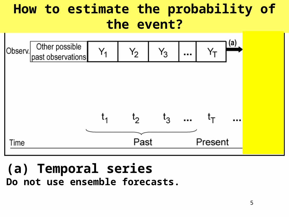
5
How to estimate the probability of the event?
(a) Temporal seriesDo not use ensemble forecasts.

6
How to estimate the probability of the event?
(b) Frequentist approach Just use ensemble forecasts (do not use past observations).

7
How to estimate the probability of the event?
(c) Bayesian approachUse ensemble forecasts and prior information about past data, expert opinion or a combination between them.

8
How to estimate the probability of the event?
(d) Calibration approachIncorporate the relationship between past observations and past ensemble forecasts.

9
• Easy to obtain.
• When and , the forecaster issues probabilities of 0 and 1 (event completely impossible or completely certain to occur).
• There is no estimate of uncertainty on the predicted probability.
• The probabilities take only a finite set of discrete values.
It is unlikely the forecaster really believes this statement !!
0tn mnt
1) Frequentist approach The probability is estimated by the relative frequency:
m
n|n(Y|np ttttt )1Prˆ
= Probability that the event is observed to occur (unknown).

10
2) Bayesian approach : provides us with a posterior distribution of the predicted probability.
• Estimate a distribution a priori including the uncertainty in the parameters: )(Fpt
• Model uncertainty of the ensemble forecasts (likelihood) as a conditional distribution: )Pr( tt|pn
)|Pr()Pr()|Pr( ttttt pnpnp • Obtain a posterior distribution (Bayes’ theorem):
)|(~| tttt npBernY
)(~ tt pBerY
Davison A. C.,Cambridge University Press (2003)
)|()1Pr( tttt npE|nY
If the model is perfectly calibrated, the probability that an ensemble member forecast the event is also . ),(~| ttt pmBinpntp

11
2) Beta approach Observations
Beta(0.5,0.5) Beta(1,1) Beta(2,2) Beta(10,20)
Katz and Ehrendorfer, Weather and Forecasting (2005).
Forecasts
+
choose a Prior distribution likelihood
p.d
.f.
Bet
a(
,)
),(~ Betapt ),(~| ttt pmBinpn
Posterior distribution
Bayes´ theorem ),(~| tttt nmnBetanp
But both and are unknown !!
m
nt
)|(ˆ tttt npE|np

12
How to choose the prior distribution?
2) Calculate:
• a central point:
• a measure of the spread:
= weight, = Number of past observations
The weight gives different importance to prior belief and model forecasts and is chosen to minimize the logarithmic score.
wmT
wnYT|n(Y ttt
)1Pr
m
nnYP ttt )|1(
Y
?
Rajagopalan et al. (2002) method is a particular case, where: w
T
w T
= = 0 . This is equivalent to the frequentist approach.
= climatology
13
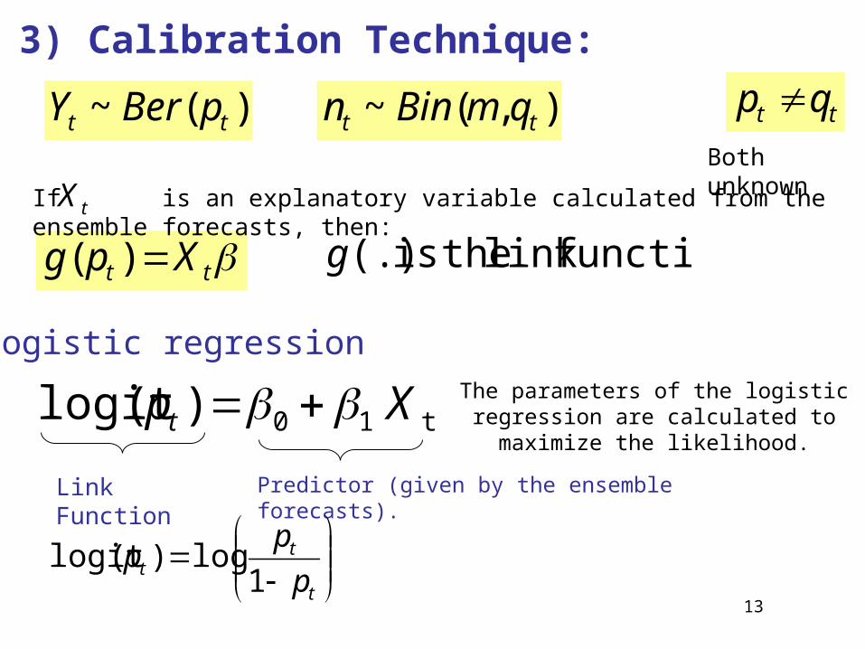
3) Calibration Technique:
Both unknown
)(~ tt pBerY ),(~ tt qmBinn tt qp
Predictor (given by the ensemble forecasts).Link Function
The parameters of the logistic regression are calculated to maximize the likelihood.
t
tt p
pp
1log)(logit
t10 )(logit Xpt Logistic regression
tt Xpg )( functionlink theis (.)g
If is an explanatory variable calculated from the ensemble forecasts, then:tX
14
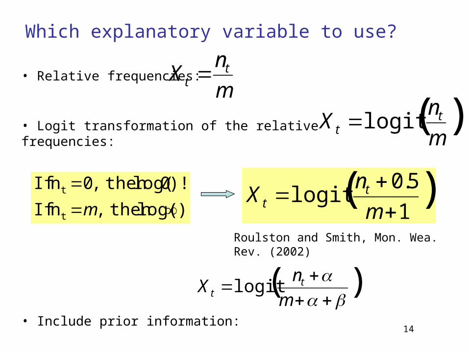
• Relative frequencies:
• Logit transformation of the relative frequencies:
• Include prior information:
Which explanatory variable to use?
Roulston and Smith, Mon. Wea. Rev. (2002)
)!log( then ,n If
)!0log( then ,0n If
t
t
m
)( logitm
nX tt
)( 1
5.0logit
m
nX tt
m
nX tt
)(logit
m
nX tt

15
1)Relative frequencies
2) Beta approach
Rajagopalan et al. (2002)
3) Logistic Regression
Summary of methods
m
n|np ttt ˆ
m
n|np tttˆ
Twm
YTwn|np ttt
ˆ
)ˆˆexp(1
)ˆˆexp(ˆ
10
10
t
ttt
X
X|np
' , mY

16
Example: Daily winter precipitation at Reading (UK)
Forecasts: 3-day ahead 50-member forecasts of daily total precipitation from Ensemble Prediction System (EPS) at ECMWF for a grid point near Reading (UK) forecast
Period: Dec-Jan-Feb from 1997 to 2006.
n= 812 daily observations
m x n = 50 x 812 = 40600 forecasts
Binary event: precipitation above a threshold.
Observations: total daily precipitation observed at the University of Reading atmospheric observatory.

17
)(nsObservatio mm
Precipitation in Reading:
The model is not perfectly calibrated
0.1 mm (WMO def.of wet day)
2 mm (perc= 75.6%)
10 mm (perc.=97%, extreme event).

180.0 0.2 0.4 0.6 0.8 1.0
0.0
0.2
0.4
0.6
0.8
1.0
pt
pt^ |
n t
climFreq.RZLLog.Reg. qtLog.Reg.logit(qt)
0.0 0.2 0.4 0.6 0.8 1.0
0.0
0.2
0.4
0.6
0.8
1.0
pt
pt^ |
n t
climFreq.RZLLog.Reg. qtLog.Reg.logit(qt)
0.0 0.2 0.4 0.6 0.8 1.0
0.0
0.2
0.4
0.6
0.8
1.0
pt
pt^ |
n t
climFreq.RZLLog.Reg. qtLog.Reg.logit(qt)
Th
resh
old
=0
.1m
mT
hre
sho
ld=
10
mm
Th
resh
old
=2
mm
The predicted probability can be expressed as a function of the frequency approach:
F is a lineal function in the RLZ method and non linear in the Logistic Regression approach.
tt|np̂
)(ˆm
nF|np t
tt
mnt /
mnt / mnt /

19
BRIER SCORE 0.1 mm 2 mm 10 mm
Climatology 0.249 0.185 0.0390
Frequencies 0.265 0.117 0.0367
Bayesian approach (RLZ) 0.218 0.111 0.0319
Log. Reg. (Xt = qt) 0.189 0.109 0.0318
Log. Reg. (Xt = logit qt) 0.189 0.108 0.0312
Brier Score:
T
ttt Yp
TBS
1
2)ˆ(1
All the BS improve the frequencies one ( =0.05).

20
Example 2: Niño-3.4 SST index
Observations: Niño-3.4 SST index
Forecasts: 5-month ahead 9-member ensemble forecasts of Niño 3.4 SST index from the coupled ECMWF model ( DEMETER).
Period: hindcasts for December started in the 1st of August of each year from 1958 to 2001.
n = 44 observations
m x n = 9 x 44 = 396 forecasts
(Palmer et al. Bull. Am. Meteorol. Soc., 2004)
Binary event: Index above the median.
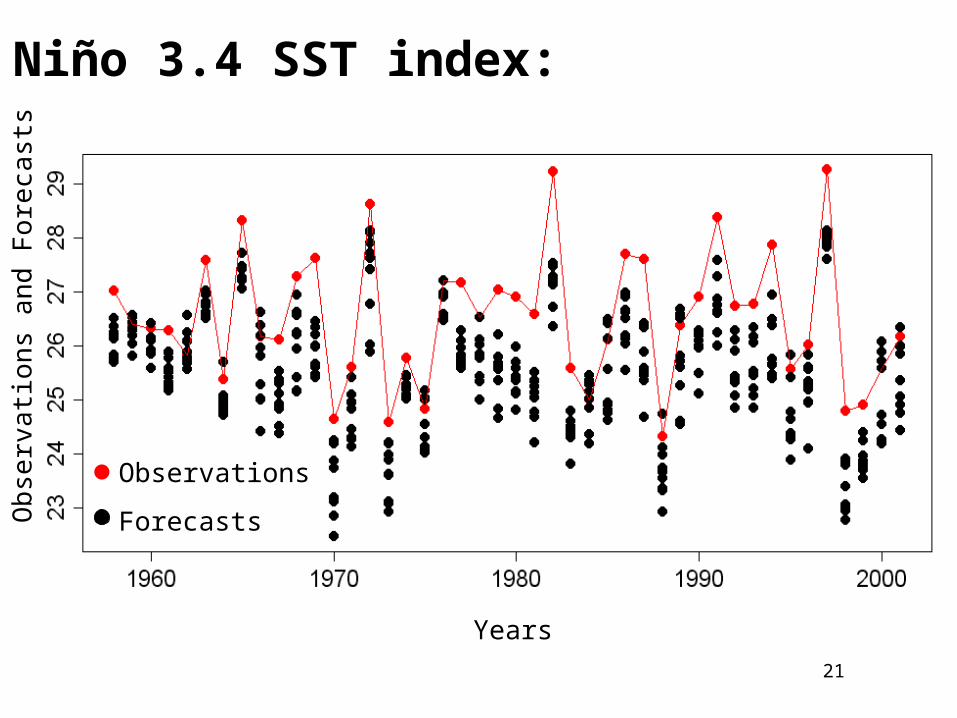
21
Years
Ob
serv
atio
ns a
nd F
ore
cast
s
Niño 3.4 SST index:
Observations
Forecasts

2222 23 24 25 26 27 28 29
22
23
24
25
26
27
28
29
Observations (mm)
Fo
reca
sts
(mm
)
Niño 3.4 SST index:
90% perc.
75% perc.
median
Median 75% 90%
We calibrate the data when we codify them.

23
Brier Score:
T
ttt Yp
TBS
1
2)ˆ(1
BRIER SCORE 0.1 mm 2 mm 10 mm
Climatology 0.5 0.187 0.1007
Frequencies 0.156 0.091 0.0171
Bayesian approach (RLZ) 0.150 0.090 0.0171
Log. Reg. (Xt = qt) 0.151 0.093 0.0114

24
Conclusions based on this example:
- Use of prior information via the Beta distribution gives forecasts that have more skill than the frequentist ones
- Calibration using logistic regression gives forecasts that have more skill than the frequentist ones
- A combination of Beta technique and calibration improves each technique separately.
Work is still necessary to choose the best predictor for the logistic regression and the best way to combine both techniques.
[email protected]://www.met.rdg.ac.uk/~sws05cp/

25
END

26