creasingbehaviourof corrugatedboard - materials … · 2006-04-24 · creasingbehaviourof...
TRANSCRIPT

Creasing behaviour ofcorrugated board
An experimental and numerical approach
L.G.J. GoorenReport MT06.06
Master’s thesis
Coach: Dr.Ir. R.H.J. Peerlings
Supervisor: Prof.Dr.Ir. M.G.D. Geers
Technische Universiteit EindhovenDepartment Mechanical EngineeringMaterials Technology
Eindhoven, February 2006


Abstract
The present study focusses on the creasing behaviour of corrugated board. To fold a board in aproper way, crease lines are applied to define the folding line and to reduce the necessary momentfor folding. The purpose of this study is to understand and predict cracking of corrugated boardduring the creasing process by means of experiments with microscopic techniques combined withnumerical simulations.
A test set-up is designed which allows one to perform creasing on small samples of paperboard inthe field of view of an Optical Microscope or a Scanning Electron Microscope (SEM). The basisfor the setup is formed by a Micro-Tensile Stage which fits in the vacuum chamber of the SEM.Special tools have been manufactured for this stage, which mimic flatbed-creasing as performed inan industrial environment. In this report we consider only the case in which the creaser is orientedin the cross direction, i.e. perpendicular to the machine direction. This orientation is the mostcritical in practice.
In the experiments no cracking is observed. However, it is observed that the inside liner is damaged,depending on the position of the creaser with respect to the flute.
Numerical simulations are used to provide insight in the stress and strain distribution. An or-thotropic (hypo-)elasticity model, as well as an anisotropic yield criterion due to Hill48, is em-ployed. Tensile tests are performed in order to determine the material properties. Due to measure-ment difficulties the out-of-plane properties are not determined experimentally, instead empiricrelations are used.
The deformations predicted by the finite element (FE) model show a good agreement with theexperiments. However, the load-displacement response predicted by the model deviates from thatin experiments. The lack of compressibility of the Hill48 yield criterion and the out-of-plane shearstress and shear yield stress have a significant influence on the creasing reaction force. The reactionforce is mainly governed by the fluting stiffness.
It is demonstrated that creasing exactly between two peaks of the fluting is the most critical case.The stress in machine direction is again influenced by the value of the out-of-plane properties,therefore a realistic stress distribution can not be given. The washboard effect, i.e. the wavinessof the liner, appear to reduces the stress in the inside liner.
i

ii
Samenvatting
Dit rapport beschrijft het rilgedrag van golfkarton. Een ril wordt gemaakt in golfkarton om eenvouwlijn aan te brengen en om het benodigde vouwmoment te verlagen. Het doel van dit onderzoekis het begrijpen van het rilgedrag en vervolgens het voorspellen van het scheuren van golfkarton.Hiervoor zijn microscopische technieken in combinatie met numerieke simulaties gebruikt.
Een experimentele opstelling is bedacht waarmee kleine proefstukjes gerild kunnen worden in hetzichtveld van een optische of een elektronen microscoop (SEM). Een op de industriële gebaseerderilsimulator is ontworpen waarmee deze rilproeven op kleine schaal uitgevoerd kunnen worden.Als basis is een Micro-Tensile Stage genomen welke in de SEM geplaatst kan worden. De toolkan op een Micro-Tensile Stage gemonteerd worden. In dit rapport zal alleen gefocust worden oprillen in de dwars richting van het papier, met andere woorden haaks op de machine richting. Inde praktijk is dit de meest kritische ril.
Daadwerkelijk scheuren is niet geconstateerd tijdens de experimenten. Desalniettemin, laat hetrillen duidelijk meer vrijgekomen vezels op de rillijn zien, wat de groei van schade impliceert.
Numerieke simulaties zijn gebruikt om inzicht te krijgen in de spanning- en rekdistributie. Een or-thotroop (hypo-)elastisch met een anisotroop vloeicriterium volgens Hill48 is gebruikt. Trekproevenzijn uitgevoerd om de materiaal eigenschappen te bepalen. Omdat de materiaal eigenschappen indikte richting moeilijk te bepalen zijn, zijn hiervoor empirische relaties gebruikt.
De vervormingen van het eindige elementen (EE) model tonen een goede overeenkomst met deexperimenten. Echter, de kracht-verplaatsing respons wijkt aanzienlijk af van de experimenten.Het ontbreken van compressibiliteit van het Hill48 vloeicriterium en de invloed van de afschuif-modulus en de afschuifvloeigrens beïnvloeden het verloop van de reactie kracht. De reactie krachtwordt voornamelijk bepaald door de stijfheid van de golf.
Het is aangetoond dat rillen tussen twee golftoppen het meest kritisch is. De spanning in machinerichting wordt mede bepaald door de materiaal eigenschappen in dikte richting. Hierdoor kan geenrealistisch beeld van spanning worden gegeven. Het zogenaamde wasbordeffect, de golving van deliner, blijkt een positieve invloed te hebben op de spanning in de liner.
iii

iv

Nomenclature
Roman symbols
Symbol Description
4C elasticity tensorD deformation rate tensorE Young’s modulusF deformation gradient tensorF,G,H,L,M,N Hill48 yield surface constantsf yield functionG shear modulusL velocity gradient tensorR ratio of yield in orthotropic direction and σref
T corrugated board thicknesstf flute thicknesstl liner thickness~x position vector~v velocity vector
Greek symbols
Symbol Description
α angleδ creaser displacementγ plastic multiplierε linear strain tensorΛ attachment lengthλ period of the flutingνij Poisson’s ratio of axial strain and lateral strainσ Cauchy stress tensorσ equivalent stressσref reference yield stressΩ spin tensor
v

General subscripts and superscripts
Symbol Description
(.)e elastic part(.)ii component in i-direction(.)ij component in ij-direction(.)p plastic part(.)ref reference state
Operators
Symbol Description
[.] components of a tensor in matrix formx material time derivative of xa · b single tensor contractionA : B double tensor contraction~∇x gradient of x
Abbreviations
Symbol Description
CD cross directionDIC digital image correlationMD machine directionZD thickness direction
vi

Contents
Abstract i
Samenvatting iii
Nomenclature v
Contents vii
1 Introduction 11.1 Corrugated board . . . . . . . . . . . . . . . . . . . . . . . . . . . . . . . . . . . . . 11.2 Creasing of corrugated board . . . . . . . . . . . . . . . . . . . . . . . . . . . . . . 21.3 Aims and scope . . . . . . . . . . . . . . . . . . . . . . . . . . . . . . . . . . . . . . 3
2 Mechanical behaviour of paper 52.1 Paper as a fibrous material . . . . . . . . . . . . . . . . . . . . . . . . . . . . . . . 52.2 Bonds in paper . . . . . . . . . . . . . . . . . . . . . . . . . . . . . . . . . . . . . . 62.3 Stress-strain response . . . . . . . . . . . . . . . . . . . . . . . . . . . . . . . . . . 7
2.3.1 In-plane behaviour . . . . . . . . . . . . . . . . . . . . . . . . . . . . . . . . 72.3.2 Out-of-plane behaviour . . . . . . . . . . . . . . . . . . . . . . . . . . . . . 8
3 Constitutive model 113.1 Kinematics . . . . . . . . . . . . . . . . . . . . . . . . . . . . . . . . . . . . . . . . 113.2 The constitutive model . . . . . . . . . . . . . . . . . . . . . . . . . . . . . . . . . . 12
3.2.1 Elastic deformation . . . . . . . . . . . . . . . . . . . . . . . . . . . . . . . . 123.2.2 Elasto-plastic deformation . . . . . . . . . . . . . . . . . . . . . . . . . . . . 12
3.3 Hill48 yield criterion . . . . . . . . . . . . . . . . . . . . . . . . . . . . . . . . . . . 13
4 Experimental identification of the orthotropic material constants 174.1 Tensile test set-up and preparation . . . . . . . . . . . . . . . . . . . . . . . . . . . 174.2 In-plane behaviour . . . . . . . . . . . . . . . . . . . . . . . . . . . . . . . . . . . . 18
4.2.1 Elastic parameters . . . . . . . . . . . . . . . . . . . . . . . . . . . . . . . . 194.2.2 Plastic parameters . . . . . . . . . . . . . . . . . . . . . . . . . . . . . . . . 20
4.3 Out-of-plane behaviour . . . . . . . . . . . . . . . . . . . . . . . . . . . . . . . . . . 214.3.1 Elastic parameters . . . . . . . . . . . . . . . . . . . . . . . . . . . . . . . . 214.3.2 Plastic parameters . . . . . . . . . . . . . . . . . . . . . . . . . . . . . . . . 21
4.4 Summary of material constants . . . . . . . . . . . . . . . . . . . . . . . . . . . . . 224.5 Numerical in-plane tensile test . . . . . . . . . . . . . . . . . . . . . . . . . . . . . 22
vii

CONTENTS
5 Creasing experiments 255.1 Creasing in real-life and experimental creasing . . . . . . . . . . . . . . . . . . . . . 255.2 Creasing set-up . . . . . . . . . . . . . . . . . . . . . . . . . . . . . . . . . . . . . . 265.3 Experimental creasing . . . . . . . . . . . . . . . . . . . . . . . . . . . . . . . . . . 26
5.3.1 Position I . . . . . . . . . . . . . . . . . . . . . . . . . . . . . . . . . . . . . 275.3.2 Position II . . . . . . . . . . . . . . . . . . . . . . . . . . . . . . . . . . . . . 275.3.3 Position III . . . . . . . . . . . . . . . . . . . . . . . . . . . . . . . . . . . . 28
5.4 Creasing with liner plate . . . . . . . . . . . . . . . . . . . . . . . . . . . . . . . . . 29
6 Confrontation of simulations vs experiments 356.1 Model definition . . . . . . . . . . . . . . . . . . . . . . . . . . . . . . . . . . . . . 356.2 Simulations with reference parameters . . . . . . . . . . . . . . . . . . . . . . . . . 36
6.2.1 Position I . . . . . . . . . . . . . . . . . . . . . . . . . . . . . . . . . . . . . 376.2.2 Position II . . . . . . . . . . . . . . . . . . . . . . . . . . . . . . . . . . . . . 386.2.3 Position III . . . . . . . . . . . . . . . . . . . . . . . . . . . . . . . . . . . . 39
6.3 Comparison of inner liner stress . . . . . . . . . . . . . . . . . . . . . . . . . . . . . 396.4 Influence of material and geometric properties . . . . . . . . . . . . . . . . . . . . . 40
6.4.1 Material properties . . . . . . . . . . . . . . . . . . . . . . . . . . . . . . . . 406.4.2 Geometric properties . . . . . . . . . . . . . . . . . . . . . . . . . . . . . . . 42
6.5 Influence of boundary conditions . . . . . . . . . . . . . . . . . . . . . . . . . . . . 436.6 Summary of observations . . . . . . . . . . . . . . . . . . . . . . . . . . . . . . . . 44
7 Conclusion and recommendations 47
Bibliography 49
Appendices 51
A Hill48 detailed calculations 53
B Calculation of in-plane shear 55
C Crease simulations overview 57
Dankwoord 59
viii

Chapter 1
Introduction
1.1 Corrugated board
We all know corrugated board as used in boxes, but its origin is surprisingly different. In the19th century, hand-cranked corrugated roller presses were used to generate corrugated paper.Corrugated paper replaced the plain paper which was used to keep the shape of the tall, stiff hatsworn by gentlemen. The new cylinder was stronger than plain paper. Later, corrugated paperwas first used to wrap bottles and slowly the first boxes were introduced. These boxes were muchlighter and less expensive than the original ones made out of solid board.
Nowadays, paper and paperboard are commonly used materials in nearly every industry. World-wide about 300 million metric tons of paper and paperboard are produced each year. Probablythe most important structural application are corrugated containers. Corrugated packaging is aversatile, economic, light, robust, recyclable, practical and yet appealing form of packaging. It istypically lightweight and inexpensive, with high stiffness-to-weight and strength-to-weight ratios.In figure 1.1 a piece of corrugated board is presented.
Figure 1.1: An example of a cardboard box at different scales
Corrugated board panels are sandwich structures consisting of two flat sheets, called liners, whichare separated by a wave shaped core, called the fluting. These three layers of paper are assembledaccording the procedure presented in figure 1.2. Its specific structure gives the board a muchbetter resistance against bending than that of each distinct layer.
1

CHAPTER 1. INTRODUCTION
Figure 1.2: The manufacturing of a single wall corrugated board [1].
1.2 Creasing of corrugated board
Creasing of corrugated board is an important technique used in the production of e.g. boxes. Tofold a board in a proper way, crease lines are applied to define the folding line and to reduce thenecessary moment to create a fold.
When board is creased by a creaser, permanent deformation is induced. Locally it decreasesthe stiffness and the board is easily bent along the crease line. The local deformation causes anincrease of stress and eventually may result in cracking of the board. Figure 1.3 shows a part ofan unfolded box which contains a crack in the inside liner.
Cracking of the outside liner also occurs. This is not caused by the creasing process. It occursafter the folding process. Board sheets are folded in a way to minimize storage space, so 180degrees folds are commonly applied. When board sheets are piled up, the 180 degrees folds maycause cracking of the outside liner.
Both failures are not desired, because they strongly decrease the stiffness of the structure [1].Humidity and temperature vary during the seasons in the papermaking process. In practice it isnoticed that this influences the mechanical behaviour of paper and causes more cracking duringthe winter season.
Figure 1.3: A piece of corrugated board with creases and cuts. Cracking has occurred in the creasein the inside liner. The problem mainly occurs normal to the fluting. MD and CD representrespectively the machine direction and the cross direction.
2

CHAPTER 1. INTRODUCTION
1.3 Aims and scope
This project is carried out as a part of the project ’Lightweight Paper and Board’ which aims atreducing the necessary grammage for paper and board for packaging applications. This will bedone by focussing on the parameters which influence the creasing and folding of the board andthe influence of the microstructure of the paper.
The present study focusses on the creasing behaviour of corrugated board. The purpose of thisstudy is to understand and predict cracking of corrugated board during the creasing process bymeans of experiments with microscopic techniques combined with numerical simulations. Withthe use of microscopic techniques the creasing process can be visualized, thus providing insightin the process at various scales. The numerical simulations are used to model the experiments.Varying the parameters of the numerical model reveals the relevant parameters of its creasingprocess.
This report starts with an extensive introduction into the mechanical behaviour of paper (chapter2). First paper is presented as a fibrous material. The structure and bonding of paper is explained.Subsequently, stress-strain curves are shown to provide insight in the mechanical behaviour.
Chapter 3 starts with the necessary kinematics and describes the constitutive model used in thesimulations. The model combines orthotropic elasticity and orthotropic plasticity. Tensile testare performed in order to obtain the material constants. Chapter 4 describes the experimentaltechniques used to obtain the constants.
Chapter 5 describes the crease experiments which are carried out to provide insight in the process.In order to enable direct observations at various scales a creasing tool is designed, which allowsone to perform creasing operations on small samples of corrugated board in the field of view of aScanning Electron Microscope (SEM).
Finite element simulations are conducted to model the experiments in chapter 6. The simulationsare compared with the experimental creasing tests in order to investigate the ability of the modelto capture the experimentally observed response.
In chapter 7, finally, conclusions are drawn based on a confrontation of experimental and compu-tational results.
3

CHAPTER 1. INTRODUCTION
4

Chapter 2
Mechanical behaviour of paper
This chapter describes the mechanical behaviour of paper. This behaviour is of importance forthe constitutive modelling of the paper layers in the corrugated board. First, the (molecular)structure and bonding of paper is presented. Subsequently, its stress-strain response is discussed.
2.1 Paper as a fibrous material
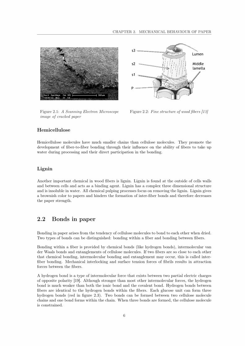
Paper mainly consists of wood fibers; however nonfiberous materials are added to provide addi-tional properties. Figure 2.1 shows a Scanning Electron Micrograph of fibers in a cracked papersheet. The precise composition depends on the grade of paper being manufactured. Wood pulpsare classified according to their method of manufacture and the wood species used. These twofactors determine the chemical composition, structure, and condition of the pulp fibers which, inturn, influence the properties of paper produced from the fibers.
Wood pulp is by far the most important source of fibers. Two main groups can be specified:softwoods (or conifers) and hardwoods (or deciduous trees). They differ in their structure, suchas fiber length. Softwoods and hardwoods have fiber lengths of respectively 3-5 mm and 1-2 mmand are respectively 20 - 80 µm and less than 20 µm in diameter [2]. Fibers in softwood providestrength and conduct fluids. Hardwood species gain strength from fibers, but have other elementsto conduct fluids (called vessel elements). Hardwood and softwood fibers have similar shapes.
Figure 2.2 shows the structure of a wood fiber. The fiber wall consists of four layers. Layer P(primary wall), layer S1 (secondary 1 layer), S2 (usually the thickest layer) and S3. The hole inthe middle is called lumen. The region surrounding the fiber is the middle lamella. In the S2 layerfibrils spiral around the fiber axis. Fibrils are small bundles of primarily cellulose molecules.
Wood fibers consist mainly of three classes materials: cellulose, hemicellulose and lignin.
Cellulose
Wood fibers are mainly built of cellulose (C6H10O5)n. Cellulose is a polymer which is madeof a linear repetition (about 5000 to 10000 times) of the monomer glucose (β-glucose). Theattraction between cellulose molecules in different fiber surfaces is the principal source of fiber-to-fiber bonding in paper.
5
CHAPTER 2. MECHANICAL BEHAVIOUR OF PAPER
Figure 2.1: A Scanning Electron Microscopeimage of cracked paper
Figure 2.2: Fine structure of wood fibers [13]
Hemicellulose
Hemicellulose molecules have much smaller chains than cellulose molecules. They promote thedevelopment of fiber-to-fiber bonding through their influence on the ability of fibers to take upwater during processing and their direct participation in the bonding.
Lignin
Another important chemical in wood fibers is lignin. Lignin is found at the outside of cells wallsand between cells and acts as a binding agent. Lignin has a complex three dimensional structureand is insoluble in water. All chemical pulping processes focus on removing the lignin. Lignin givesa brownish color to papers and hinders the formation of inter-fiber bonds and therefore decreasesthe paper strength.
2.2 Bonds in paper
Bonding in paper arises from the tendency of cellulose molecules to bond to each other when dried.Two types of bonds can be distinguished: bonding within a fiber and bonding between fibers.
Bonding within a fiber is provided by chemical bonds (like hydrogen bonds), intermolecular vander Waals bonds and entanglements of cellulose molecules. If two fibers are so close to each otherthat chemical bonding, intermolecular bonding and entanglement may occur, this is called inter-fiber bonding. Mechanical interlocking and surface tension forces of fibrils results in attractionforces between the fibers.
A hydrogen bond is a type of intermolecular force that exists between two partial electric chargesof opposite polarity [19]. Although stronger than most other intermolecular forces, the hydrogenbond is much weaker than both the ionic bond and the covalent bond. Hydrogen bonds betweenfibers are identical to the hydrogen bonds within the fibers. Each glucose unit can form threehydrogen bonds (red in figure 2.3). Two bonds can be formed between two cellulose moleculechains and one bond forms within the chain. When three bonds are formed, the cellulose moleculeis constrained.
6
CHAPTER 2. MECHANICAL BEHAVIOUR OF PAPER
CH OH2
C
C
C C
H
H
H
HOH
OH
O
C
O O
CH OH2
C
C
C C
H
H
H
HOH
OH
O
C
O
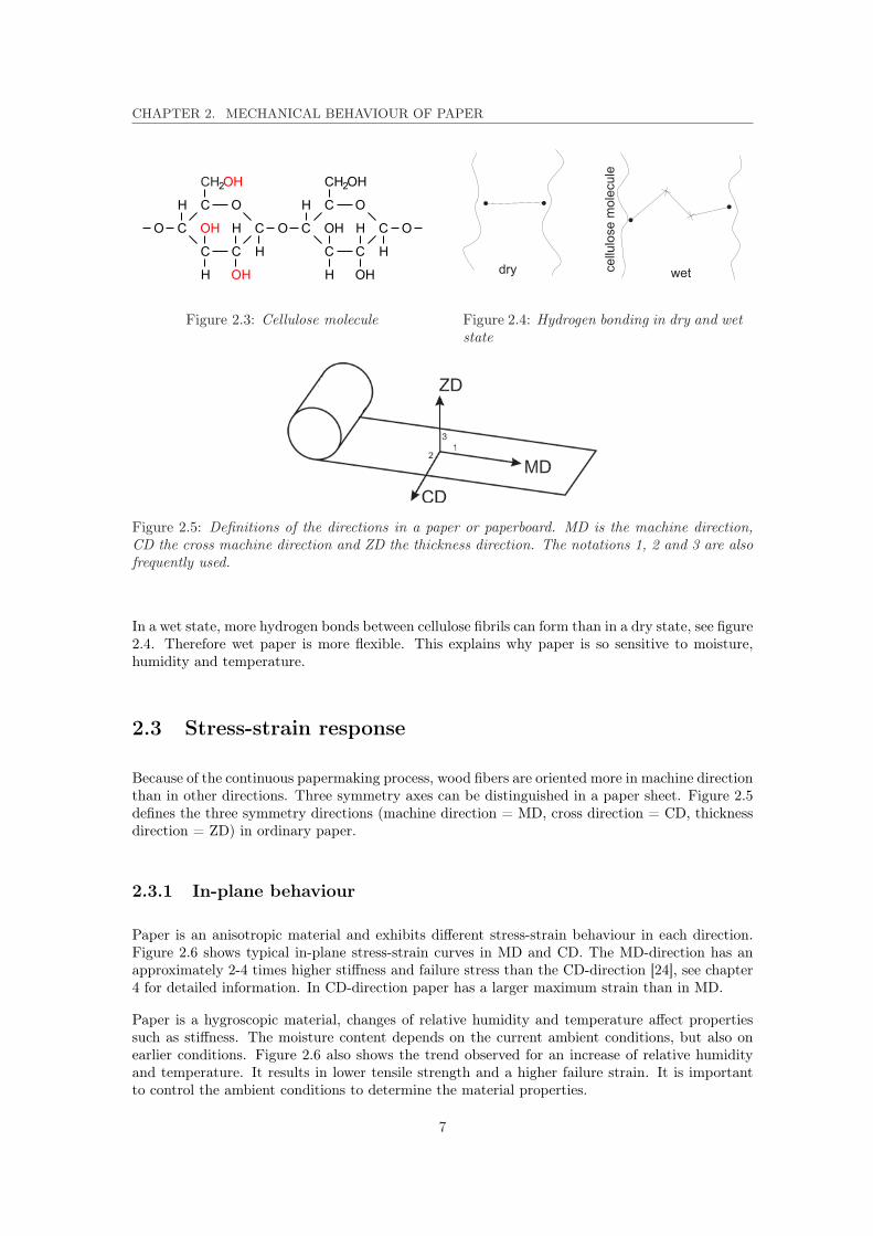
Figure 2.3: Cellulose molecule Figure 2.4: Hydrogen bonding in dry and wetstate
Figure 2.5: Definitions of the directions in a paper or paperboard. MD is the machine direction,CD the cross machine direction and ZD the thickness direction. The notations 1, 2 and 3 are alsofrequently used.
In a wet state, more hydrogen bonds between cellulose fibrils can form than in a dry state, see figure2.4. Therefore wet paper is more flexible. This explains why paper is so sensitive to moisture,humidity and temperature.
2.3 Stress-strain response
Because of the continuous papermaking process, wood fibers are oriented more in machine directionthan in other directions. Three symmetry axes can be distinguished in a paper sheet. Figure 2.5defines the three symmetry directions (machine direction = MD, cross direction = CD, thicknessdirection = ZD) in ordinary paper.
2.3.1 In-plane behaviour
Paper is an anisotropic material and exhibits different stress-strain behaviour in each direction.Figure 2.6 shows typical in-plane stress-strain curves in MD and CD. The MD-direction has anapproximately 2-4 times higher stiffness and failure stress than the CD-direction [24], see chapter4 for detailed information. In CD-direction paper has a larger maximum strain than in MD.
Paper is a hygroscopic material, changes of relative humidity and temperature affect propertiessuch as stiffness. The moisture content depends on the current ambient conditions, but also onearlier conditions. Figure 2.6 also shows the trend observed for an increase of relative humidityand temperature. It results in lower tensile strength and a higher failure strain. It is importantto control the ambient conditions to determine the material properties.
7

CHAPTER 2. MECHANICAL BEHAVIOUR OF PAPER
0 0.005 0.01 0.015 0.02 0.025 0.03 0.035 0.04 0.0450
5
10
15
20
25
30
35
40
45
strain [−]
stre
ss [M
Pa]
MD
CD
increase of RH and T
σf
σf
E2
E1
0 100 200 300 400 5000
5
10
15
20
25
30
35
40
displacement [µm]
forc
e [N
]
MD
CD
Figure 2.6: Typical in-plane stress-straincurves of paper. Ei indicates stiffness mod-ulus in i-direction, σf is the failure strength.The arrows and dashed curves show thetrend observed for an increase in humidityor temperature.
Figure 2.7: Initial non-linearity of the load-displacement curves
Near the origin, the curves exhibit non-linearity, figure 2.7. During the initial phase of the tensiletest not all the fibers are under tension. Gradually all the fibers are loaded and the load increasesaccording to a more or less constant slope. It is advised to pre-tension a tensile specimen to removethis effect [10].
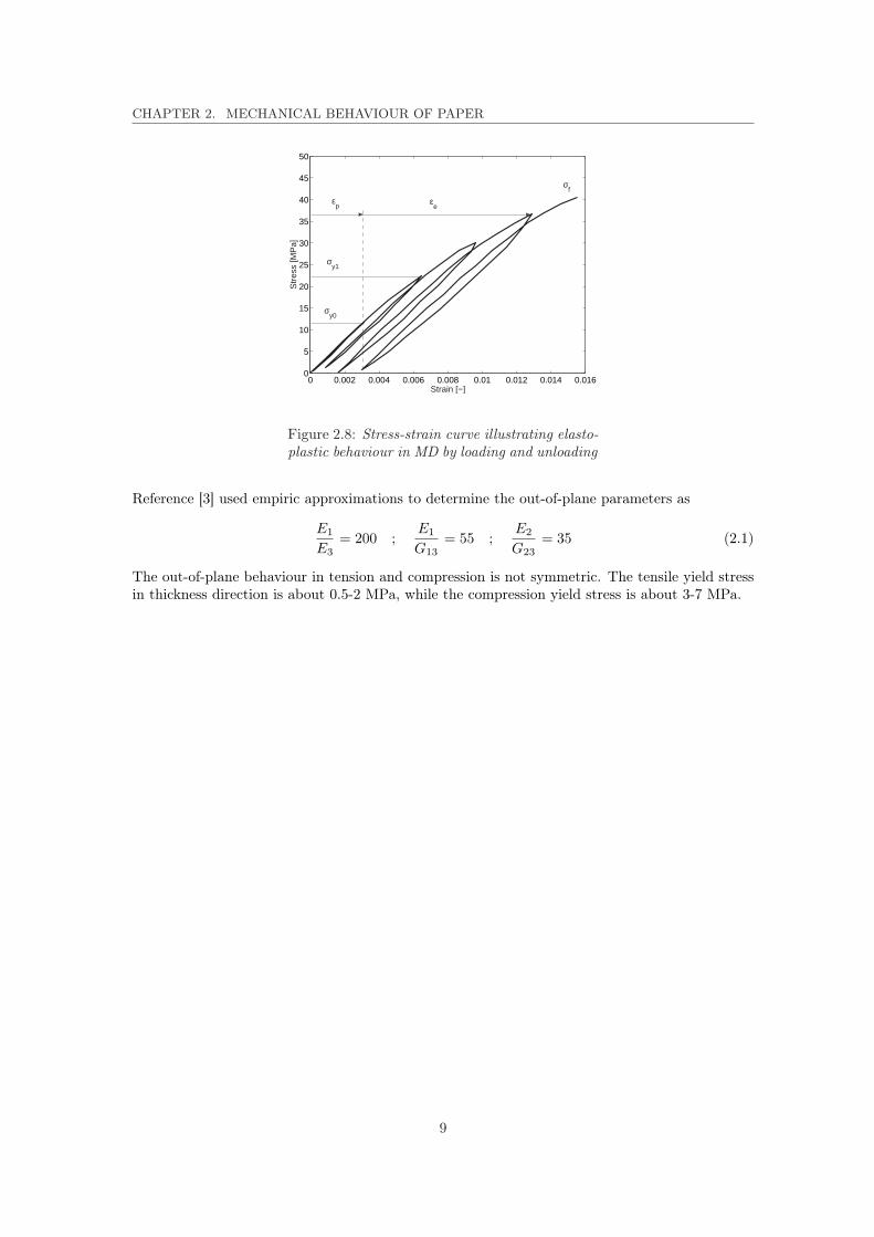
Linearity at the beginning of the stress-strain curves can be noticed. After a certain point thestress-strain curve gradually deviates from the initial slope. After the yielding point non-linearplasticity is invoked, see figure 2.8. The figure shows a stress-strain curve in MD with sequentialloading and unloading of the tensile specimen. The figure shows that paper exhibits no clear yieldpoint. Instead, the stress-strain curve gradually deviates from the initial slope. The tensile curvescan be decomposed in an elastic and plastic part (ε = εe + εp). The plastic strain and the yieldstress, σy, increase with ongoing tensile loading.
Yielding in paper is not symmetric in tension and compression. In compression, paper is less stiffthan in tension [24] and exhibits about 65% and 25% of the tensile yield stress in, respectively,MD and CD.
Paper material is strain rate dependent. It is stiff and brittle at high strain rates and weak andductile at low strain rates. However, [7] shows that in case of creasing the influence of strain ratecan be neglected.
2.3.2 Out-of-plane behaviour
The in-plane tensile properties of paper are relatively easy to determine by tensile tests. Due tothe small thickness of paper sheets, the out-of-plane properties are harder to obtain.
Reference [21] shows that the Young’s modulus in ZD-direction is about 200 times lower thanthe MD-direction. [22] observed that the amount of lateral in-plane strain generated during thethrough-thickness tensile loading is negligible. Poisson’s ratios ν31 and ν32 therefore are close tozero.
8
CHAPTER 2. MECHANICAL BEHAVIOUR OF PAPER
0 0.002 0.004 0.006 0.008 0.01 0.012 0.014 0.0160
5
10
15
20
25
30
35
40
45
50
Strain [−]
Str
ess
[MP
a]
σf
εp ε
e
σy0
σy1
Figure 2.8: Stress-strain curve illustrating elasto-plastic behaviour in MD by loading and unloading
Reference [3] used empiric approximations to determine the out-of-plane parameters as
E1
E3= 200 ;
E1
G13= 55 ;
E2
G23= 35 (2.1)
The out-of-plane behaviour in tension and compression is not symmetric. The tensile yield stressin thickness direction is about 0.5-2 MPa, while the compression yield stress is about 3-7 MPa.
9

CHAPTER 2. MECHANICAL BEHAVIOUR OF PAPER
10
Chapter 3
Constitutive model
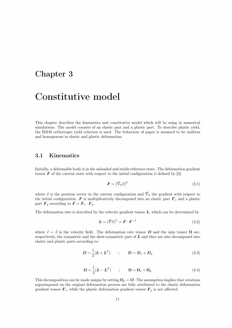
This chapter describes the kinematics and constitutive model which will be using in numericalsimulations. The model consists of an elastic part and a plastic part. To describe plastic yield,the Hill48 orthotropic yield criterion is used. The behaviour of paper is assumed to be uniformand homogenous in elastic and plastic deformation.
3.1 Kinematics
Initially, a deformable body is in the unloaded and stable reference state. The deformation gradienttensor F of the current state with respect to the initial configuration is defined by [5]:
F = (~∇0~x)T (3.1)
where ~x is the position vector in the current configuration and ~∇0 the gradient with respect tothe initial configuration. F is multiplicatively decomposed into an elastic part F e and a plasticpart F p according to F = F e · F p.
The deformation rate is described by the velocity gradient tensor L, which can be determined by
L = (~∇~v)T = F · F−1 (3.2)
where ~v = ~x is the velocity field. The deformation rate tensor D and the spin tensor Ω are,respectively, the symmetric and the skew-symmetric part of L and they are also decomposed intoelastic and plastic parts according to:
D =12(L + LT ) ; D = De + Dp (3.3)
Ω =12(L−LT ) ; Ω = Ωe + Ωp (3.4)
This decomposition can be made unique by setting Ωp = O. The assumption implies that rotationssuperimposed on the original deformation process are fully attributed to the elastic deformationgradient tensor F e, while the plastic deformation gradient tensor F p is not affected.
11

CHAPTER 3. CONSTITUTIVE MODEL
3.2 The constitutive model
The constitutive model consists of two parts, an elastic and a plastic part. In the initial state, onlyelastic deformation can occur. While the stress rises a yield criterion, f , indicates the transition toplasticity. Kuhn-Tucker relations are used to decide whether elastic or elasto-plastic deformationoccurs.
(f < 0) ∨ (f = 0 ∧ f < 0) → elastic deformation(f = 0) ∧ (f = 0) → elasto-plastic deformation (3.5)
3.2.1 Elastic deformation
When the deformation is purely elastic, Dp = 0, so De = D. The objective Jaumann rate of theCauchy stress tensor is related to the elastic deformation rate De by
σ= 4C : De (3.6)
4C is the fourth order stiffness tensor.
As argued in chapter 2, paper is made of oriented wood fibers and elastic stiffness and strengthare therefore anisotropic. If we assume the fiber distribution to be symmetric, the stiffness prop-erties are orthotropic. The orthotropic linear elastic stiffness tensor is defined (in compact matrixnotation) as
C =
E−11 −ν21E
−12 −ν31E
−13 0 0 0
−ν12E−11 E−1
2 −ν32E−13 0 0 0
−ν13E−11 −ν23E
−12 E−1
3 0 0 00 0 0 G−1
12 0 00 0 0 0 G−1
23 00 0 0 0 0 G−1
31
−1
(3.7)
Due to the symmetry of C, the material parameters must obey the three Maxwell relationsν12
E1=
ν21
E2;
ν23
E2=
ν32
E3;
ν31
E3=
ν13
E1(3.8)
νij is equal to minus the ratio of the transverse strain in the j -direction and the axial strainin the i -direction when the material is uniaxially stressed in i -direction. Additionally, positivedefiniteness of C requires [26]
E1, E2, E3, G12, G23, G31 > 0
|ν12| <(
E1E2
) 12
|ν13| <(
E1E3
) 12
|ν23| <(
E2E3
) 12
1− ν12ν21 − ν23ν32 − ν31ν13 − 2ν21ν32ν12 > 0
(3.9)
The orthotropic elasticity tensor now contains nine independent parameters, E1, E2, E3, ν12, ν13,ν23, G12, G13, G23, which have to be measured.
3.2.2 Elasto-plastic deformation
In elasto-plastic material models a yield function defines whether the response is elastic or elasto-plastic. As long as the stress state has not reached the threshold f = 0 defined by the yield
12

CHAPTER 3. CONSTITUTIVE MODEL
function f (σ, εp) the behaviour is elastic. f is defined as
f (σ, εp) = σ2 − σ2y(εp) (3.10)
with σ2 a quadratic form of the stress tensor and σy the yield stress defined as
σy = σy(σy0, εp) (3.11)
The hardening modulus H is defined as
∂σy
∂εp= H(εp) (3.12)
The yield stress increases due to hardening as the plastic deformation continues and is thereforerelated to the effective plastic strain εp:
εp =∫ t
τ=0
εpdτ ; εp =
√23Dp : Dp (3.13)
Plastic flow is assumed to obey normality, i.e. we use the associative flow rule:
Dp = γ∂f
∂σ(3.14)
Dp is characterized by the plastic multiplier, γ. In order to obtain the plastic multiplier theconsistency condition for plasticity (f = 0) is used.
3.3 Hill48 yield criterion
Several material models to describe paper have been developed in the past years, [3] [21] [24]. Apopular criterion which describes orthotropic plasticity is the Hill48 quadratic yield criterion.
Hill [11] proposed an orthotropic yield function as an extension of the Von Mises yield function.This yield criterion is commonly applied in sheet metal applications and is insensitive to hydrostaticpressure, or mean stress. The plastic strain rate is normal to the yield surface and therefore noplastic volume change is invoked. Hill48 does not distinguish between tension and compression,so tensile and compressive yield occur at ±σiiy.
[21] and [24] propose a model with orthotropic elastic behaviour and an orthotropic yield surfaceconstructed from sub-surfaces with orthotropic hardening. An extended Hill48 criterion whichallows volume change during plastic deformation is proposed. Each proposed model assumesuniform and homogenous elastic and plastic deformation.
Hill48 is provided as an option in MSC.MARC/MENTAT 2005 and is used as a first approximationfor describing orthotropic yield. The general yield criterion can be written as [11] [15]
f = F(σ22 − σ33)2 + G(σ33 − σ11)2 +H(σ11 − σ22)2 + 2Lσ2
23 + 2Mσ231 + 2Nσ2
12 − 1 (3.15)
where the subscript ii indicates the stress and ij indicates the shear stress in the principal directionsof orthotropy. F, G, H, L, M and N characterize the anisotropy of the material. Note that bytaking F, G and H equal to 1 and L, M and N equal to 3, the Hill function degenerates to the
13

CHAPTER 3. CONSTITUTIVE MODEL
Von Mises yield function. The constants F, G, H, L, M and N are defined as
2F =1
σ222y
+1
σ233y
− 1σ2
11y
; 2L =1
σ223y
2G =1
σ211y
+1
σ233y
− 1σ2
22y
; 2M =1
σ231y
(3.16)
2H =1
σ211y
+1
σ222y
− 1σ2
33y
; 2N =1
σ212y
with σijy the yield stress values in ij-direction. Rearranging (3.16) gives
1σ2
11y
= G + H ;1
σ222y
= F + H ;1
σ233y
= F + G (3.17)
It is clear that the constants F-N must satisfy
(F + G), (G + H), (F + H) > 0, L, M, N > 0 (3.18)
[12] also shows that the constant have to obey
FG + GH + HF > 0 (3.19)
in order for the yield surface to be convex. Note that this condition leaves open the possibilitythat one of F, G and H may be negative.
Instead of the constants of (3.16) MSC.MARC/MENTAT 2005 uses ratios, Rij (see appendix Afor more details), of actual yield stress to isotropic yield stress, which are defined in the orthotropicdirections according to
R11 =σ11y
σref; R12 =
√3σ12y
σref
R22 =σ22y
σref; R13 =
√3σ13y
σref(3.20)
R33 =σ33y
σref; R23 =
√3σ23y
σref
where σref is the initial yield stress derived from the stress-strain curve in a preferential direction.Here we will use σref = σ11y, which implies that R11 = 1.
Hill48 limits the degree of orthotropy in three directions. For given σ11y and σ22y, σ33y dependson σ22y and cannot be chosen arbitrarily. By substituting (3.16) and (3.21) in (3.19), rewritingthe result in terms of Rii and setting R11 = 1 it can be shown that R33 has to satisfy (see alsoappendix B)
R22
(1 + R22)< R33 <
R22
(1−R22)(3.21)
Figure 3.1 shows a range of R22 with the limitations imposed on R33 by these inequalities.
14

CHAPTER 3. CONSTITUTIVE MODEL
0 0.2 0.4 0.6 0.8 10
0.1
0.2
0.3
0.4
0.5
0.6
0.7
0.8
0.9
1
R22
R33
Figure 3.1: Limitations on R33, when R11 = 1and R22 is known. For a high degree of or-thotropy, i.e. small R11, we have R22 ≈ R33.
15

CHAPTER 3. CONSTITUTIVE MODEL
16
Chapter 4
Experimental identification of theorthotropic material constants
The previous chapters described the material response of paper and proposed a constitutive modelto characterize it. This model contains several material constants which are to be determinedin this chapter. First the test set-up and preparation are described. The material constantsidentification is divided into elastic and plastic properties. The plastic hardening is also derivedfrom the tensile tests. The in-plane parameters are used in the material model and compared withthe experiments.
4.1 Tensile test set-up and preparation
A single-wall corrugated board with B flute is considered. This type of board consists of threedifferent papers. Although the three papers are not entirely identical, it was found that thereis little difference in their tensile response. Therefore only the inside liner is used for parameteridentification and the results are also used for the flute and outside liner. The specimens werekindly provided by Kappa Containerboard.
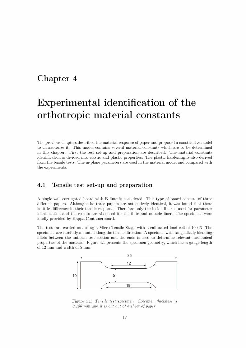
The tests are carried out using a Micro Tensile Stage with a calibrated load cell of 100 N. Thespecimens are carefully mounted along the tensile direction. A specimen with tangentially blendingfillets between the uniform test section and the ends is used to determine relevant mechanicalproperties of the material. Figure 4.1 presents the specimen geometry, which has a gauge lengthof 12 mm and width of 5 mm.
Figure 4.1: Tensile test specimen. Specimen thickness is0.186 mm and it is cut out of a sheet of paper
17
CHAPTER 4. EXPERIMENTAL IDENTIFICATION OF THE ORTHOTROPIC MATERIALCONSTANTS
The strain in the gauge section is determined by dividing the clamp displacement by an effectivegauge length of 18 mm. According to international standards for paper testing, tests have to beperformed at a constant 23oC, a constant relative humidity of 50% and a constant elongation rateof 20 mm/min ± 5 mm/min.
Since the creasing tests which we aim to model are done in a SEM, the tensile tests are also donein the SEM. One should notice that the climate in the sample chamber of the SEM will be differentfrom the international standards. The condition in the SEM is approximately 30oC and RH 0%.The paper will respond to the vacuum by evaporating all moisture.
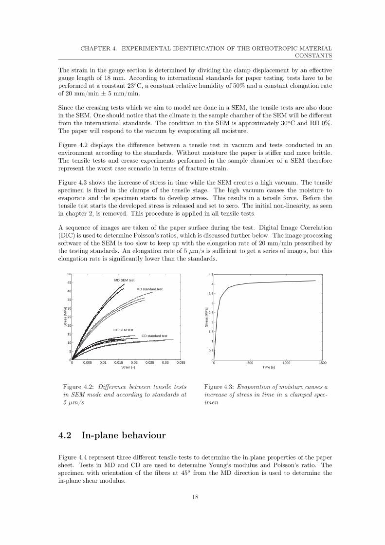
Figure 4.2 displays the difference between a tensile test in vacuum and tests conducted in anenvironment according to the standards. Without moisture the paper is stiffer and more brittle.The tensile tests and crease experiments performed in the sample chamber of a SEM thereforerepresent the worst case scenario in terms of fracture strain.
Figure 4.3 shows the increase of stress in time while the SEM creates a high vacuum. The tensilespecimen is fixed in the clamps of the tensile stage. The high vacuum causes the moisture toevaporate and the specimen starts to develop stress. This results in a tensile force. Before thetensile test starts the developed stress is released and set to zero. The initial non-linearity, as seenin chapter 2, is removed. This procedure is applied in all tensile tests.
A sequence of images are taken of the paper surface during the test. Digital Image Correlation(DIC) is used to determine Poisson’s ratios, which is discussed further below. The image processingsoftware of the SEM is too slow to keep up with the elongation rate of 20 mm/min prescribed bythe testing standards. An elongation rate of 5 µm/s is sufficient to get a series of images, but thiselongation rate is significantly lower than the standards.
0 0.005 0.01 0.015 0.02 0.025 0.03 0.0350
5
10
15
20
25
30
35
40
45
50
Strain [−]
Str
ess
[MP
a]
MD SEM test
CD SEM test
MD standard test
CD standard test
0 500 1000 15000
0.5
1
1.5
2
2.5
3
3.5
4
4.5
Time [s]
Str
ess
[MP
a]
Figure 4.2: Difference between tensile testsin SEM mode and according to standards at5 µm/s
Figure 4.3: Evaporation of moisture causes aincrease of stress in time in a clamped spec-imen
4.2 In-plane behaviour
Figure 4.4 represent three different tensile tests to determine the in-plane properties of the papersheet. Tests in MD and CD are used to determine Young’s modulus and Poisson’s ratio. Thespecimen with orientation of the fibres at 45o from the MD direction is used to determine thein-plane shear modulus.
18

CHAPTER 4. EXPERIMENTAL IDENTIFICATION OF THE ORTHOTROPIC MATERIALCONSTANTS
Figure 4.4: Experimental method to define the in-plane properties.The horizontal lines indicate the fiber orientation. δ is the applieddisplacement and F is the measured reaction force.
The uniaxial stress-strain curves for the MD, CD and orientation of the fibres at 45o from the MDdirection are plotted in figure 4.5. The stress is determined as the load divided by the initial areaof the cross section. Strain is determined as the elongation divided by the effective gauge length.These measures are thus engineering stress and strain and we limit ourselves to a geometricallylinear analysis.
The curves in figure 4.5 clearly show the expected anisotropic behaviour of paper. There is afactor 2-3 difference between Young’s modulus in MD and CD direction. The failure stress σf forMD is 3-4 times higher than that for CD. The yield stress and hardening in MD is higher thanthat in CD. The Young’s modulus, flow stress and hardening for 45o are between the two otherdirections.
0 0.005 0.01 0.015 0.02 0.0250
5
10
15
20
25
30
35
40
45
50
Strain [−]
Str
ess
[MP
a]
σf
σf
σf
MD
45o MD−CD
CD
0 0.005 0.01 0.015 0.02 0.025−10
−9
−8
−7
−6
−5
−4
−3
−2
−1
0x 10
−3
Axial strain [−]
Late
ral s
trai
n [−
]
ν21
ν12
Figure 4.5: In-plane tensile stress-straincurves.
Figure 4.6: Lateral strain vs. axial strain fortensile loading in the MD and CD.
4.2.1 Elastic parameters
The Young’s moduli E1 and E2 are directly determined by measuring the initial slope of thestress-strain curves, which are in MD and CD respectively 3950 MPa and 1650 MPa.
The Digital Image Correlation (DIC) method is used to determine the Poisson’s ratios. DIC isbased on the correlation of gray values of digital images of the undeformed and the deformed
19

CHAPTER 4. EXPERIMENTAL IDENTIFICATION OF THE ORTHOTROPIC MATERIALCONSTANTS
specimen. Using the change of gray values DIC can compute local strain.
Once the specimens are in the SEM and the tensile test starts, a sequence of images are taken ofthe paper surface. These images are used to compute local strain fields. DIC is a time-consumingprocedure. The computed strain is averaged in each direction over the total image and plotted infigure 4.6. This figure shows lateral strain vs. axial strain data for tensile loading in the MD andCD; the slopes of the curves fitted through the data are ν12 and ν21 respectively. The Maxwellrelation (3.8) holds for the values of ν12 and ν21. ν12 and ν21 are determined at respectively 0.65and 0.27 (solid lines).
With the above four known parameters, the shear modulus is deduced from the 45o curve. Usingelasticity theory and the assumption of plane stress, G12 is determined at 760 MPa, see appendixB.
4.2.2 Plastic parameters
A clear yield point is not visible in figure 4.5 because the deviation from the linear path growsgradually as the strain increases. One way to determine the yield point is to identify the stress atwhich the smooth curve deviates from a straight line beyond a certain percentage. Another way isby loading and unloading a specimen and inspecting whether there is any remaining deformationat zero stress, see figures 4.7 and 4.8. Both methods have been used and the yield stresses areapproximated at σ11y0 = 13 MPa and σ22y0 = 4 MPa. A small deviation of the yield stress canbe compensated in the hardening relation without affecting the total stress-strain response.
0 0.005 0.01 0.015 0.020
5
10
15
20
25
30
35
40
45
50
Strain [−]
Str
ess
[MP
a]
σy
0 0.005 0.01 0.015 0.020
2
4
6
8
10
12
14
16
18
20
Strain [−]
Str
ess
[MP
a]
σy
Figure 4.7: Stress-strain curve illustratingelastoplastic behaviour in MD under loadingand unloading
Figure 4.8: Stress-strain curve illustratingelastoplastic behaviour in CD under loadingand unloading
The yield stress of 45o tensile test, σ45y, can be used to determine σ12y. Using σ45y in equationA.1 for f = 0 results σ12y, see appendix B. σ12y is determined at approximately 5.6 MPa.
Figure 4.9 shows a stress-strain curve for the tensile test in MD direction. The total strain can bedecomposed as εe + εp. The yield stress as a function of the plastic strain, figure 4.10, is obtainedby the elastic strain
εp = ε− σ
E1(4.1)
Paper exhibits non-linear hardening behaviour. An exponential relation between the yield stress
20

CHAPTER 4. EXPERIMENTAL IDENTIFICATION OF THE ORTHOTROPIC MATERIALCONSTANTS
0 0.005 0.01 0.015 0.020
5
10
15
20
25
30
35
40
45
strain [−]
stre
ss [M
Pa]
E1
0 0.005 0.01 0.015 0.020
5
10
15
20
25
30
35
40
45
plastic strain [−]
stre
ss [M
Pa]
σ11y0
Figure 4.9: Elastic strain and total strain(εp = ε− εe)
Figure 4.10: Yield stress vs plastic strain
and the effective plastic strain describes this post-yield behaviour (in MD) very well:
σy = σy0(1 + Aεp)m (4.2)
with A = 3900 and m = 0.37. To simulate the most critical case, equation (4.2) is fitted tothe stress-strain curve with the lowest failure strength in figure 4.5. This equation is used inMSC.MARC/MENTAT 2005.
4.3 Out-of-plane behaviour
As described in chapter 2 it is difficult to measure the mechanical behaviour in thickness directionof the paper. In our creasing experiments the load in ZD will be mainly compressive. Reference[21] provides insight in the out-of-plane behaviour of paper, in tension and compression for similarpaper.
4.3.1 Elastic parameters
Recalling the empiric relations (2.1) [3] gives us approximated values for E3 = 20 MPa, G13 = 71MPa and G23 = 47 MPa.
DIC is used to determine the Poisson’s ratios ν13 and ν23. However, the results are not reliable. Thepaper sheet thickness is too small to apply DIC. Focussing at smaller scales with a SEM providesmore surface to apply DIC, but the strain field becomes too localized to get global results.
[22] observed that the amount of lateral in-plane strain generated during through-thickness tensileloading is negligible. Poisson’s ratios ν31 and ν32 are close to zero.
4.3.2 Plastic parameters
The out-of-plane shear yield stress σ23y and σ31y are not determined. In the literature typical shearyield stress of 0.3-1.1 MPa can be found [21]. However, as a first approximation R31 = R23 = 1 isapplied, for which we have σ31y = 7.5 MPa.
21

CHAPTER 4. EXPERIMENTAL IDENTIFICATION OF THE ORTHOTROPIC MATERIALCONSTANTS
Table 4.1: The reference parametersParameter Value S.I. unit Parameter Value Unit
E1 3950 MPa σ11y 13 MPaE2 1650 MPa σ22y 4 MPaE3 20 MPa σ33y 4 MPaν12 0.65 - σ12y 5.6 MPaν31 0.0035 - σ23y 7.5 MPaν32 0.0055 - σ31y 7.5 MPaG12 760 MPa A 3900 -G23 47 MPa m 0.37 -G31 71 MPa
Section 3.3 introduced the Hill48 yield criterion for describing yield in orthotropic materials.Equation (3.21) displays the stress coefficients which are used by MSC.MARC/MENTAT 2005.They form the ratio between yield stress in one direction and the reference yield stress. The yieldstress in MD direction is chosen as reference yield stress.
Since σ11y and σ22y have been determined, R11 and R22 are known. As discussed in chapter 3,R33 must obey equation (3.21). This restriction implies
3.06 < σ33y < 5.78 MPa (4.3)
In the literature typical values σ33y of 1-2 MPa in tension and 5-7 MPa in compression are found.Because of the uncertainty, σ33y is chosen to be equal to σ22y as a first estimate.
4.4 Summary of material constants
All material parameters are now determined and are summarized in table 4.1. It is emphasisedone more that the out-of-plane parameters are hard to determine. The influence these parametersin the creasing simulations will be investigated in chapter 6. The reference material parametersare recapitulated in table 4.1.
4.5 Numerical in-plane tensile test
The uniaxial tension data in MD, CD and for 45o has been used to fit the material properties, asdescribed before. In order to validate these fits, comparisons of the experiments and the simulatedstress-strain curves for uniaxial tensile tests in MD, CD, 45o are shown in figure 4.11. Figure4.12 displays experimental and simulated lateral strain vs. axial strain curves for MD and CDtension. A single four-node isoparametric quadrilateral element is used. The in-plane tensile testsare simulated assuming plane stress (σ33 = σ23 = σ13 = 0) and homogeneous deformation. Thisassumption invokes only the in-plane constants.
Note that the computational lateral strain vs axial strain curve for the CD (upper dashed curvein figure 4.12) deviates somewhat from the experimental data. This deviation starts at the onsetof plastic flow and is caused by the fact that the constants F −H of the Hill48 model, togetherwith incompressibility, fix this ratios and it cannot be defined independently.
The results demonstrate that the proposed model can describe the material behaviour of paper
22

CHAPTER 4. EXPERIMENTAL IDENTIFICATION OF THE ORTHOTROPIC MATERIALCONSTANTS
0 0.005 0.01 0.015 0.02 0.0250
5
10
15
20
25
30
35
40
45
50
Strain [−]
Str
ess
[MP
a]
MD
CD
45o MD−CD
0 0.005 0.01 0.015 0.02 0.025−10
−9
−8
−7
−6
−5
−4
−3
−2
−1
0x 10
−3
Axial strain [−]
Late
ral s
trai
n [−
]
ν21
ν12
Figure 4.11: Tensile test in several loadingcases. The solid lines represent the experi-mental curves and the dashed lines are fromthe numerical model
Figure 4.12: Comparison of experimentaland simulated lateral strain vs. axial strainfor MD and CD tension
over the full range of stress-strain in in-plane tension. The compression curve will be exactlythe opposite of the tension curve, because incompressibility is invoked in the Hill48 criterion. Inreality this is not true.
23

CHAPTER 4. EXPERIMENTAL IDENTIFICATION OF THE ORTHOTROPIC MATERIALCONSTANTS
24

Chapter 5
Creasing experiments
After the material properties have been determined, crease experiments are performed. Thischapter describes the crease tests which are carried out to verify the simulations presented furtheron in this report. A creasing set-up is designed, which allows one to perform creasing operationson small samples of paperboard in the field of view of a Scanning Electron Microscope (SEM) inorder to enable direct observations at various scales.
5.1 Creasing in real-life and experimental creasing
A certain force is needed to crease a board panel. The reaction force depends on the orientationof the creaser with respect to the corrugated board. Here we consider only the case in whichthe creaser is oriented in the CD and a more or less two-dimensional deformation pattern is thusobtained. This orientation is usually the most critical in practice.
During the manufacturing process of board there is no factor that regulates the position of thecrease line with respect to the fluting. The reaction force is different at each location and onelocation may be more damaging in terms of cracking than another. Several experiments aretherefore carried out at different positions. Three positions of the creaser with respect to theperiod of the fluting are considered:
Position I Exactly between two peaks of the flutingPosition II At the peak of the flutingPosition III Exactly between the peak and the valley
Figure 5.1: Creasing of corrugated board at three positions, with α as angle and δ as crease depth.
In [8] an extensive study on failure and crease depth of the liner with a similar fluting is performed.
25

CHAPTER 5. CREASING EXPERIMENTS
By increasing the crease depth δ, the angle α as indicated in figure 5.1 becomes larger and thestress in the inside liner increases.
If the fluting is infinitely stiff a crease at position III would be the most critical, because it leads tothe largest α and therefore the largest strain in the liner. In practice the flute has a finite stiffnessand may collapse. [7] already suggested that the flute around the crease zone must collapse toprevent failure of the liner. Then creasing at position I is the most critical crease, according [8].In that case cracking of the liner occurs at a depth of approximately 0.57 mm.
5.2 Creasing set-up
The creaser tool and the corrugated board which is to be creased are presented in figure 5.2. Thetool is mounted on a Micro Tensile Stage which can be placed in the vacuum chamber of a SEM.The anvil (1) and creaser (2) are each mounted on one clamp of a micro tensile tester, which canbe moved towards each other. Moving the clamps to each other forces the board (4) (dimensionshxl = 20x40 mm) against the anvil, resulting in local deformation of the board. A crease is thusmade.
In real-life creasing the board panel has a certain width which prevents folding of the board. Inthe experiments the specimens are too small to resist bending and down holders are added to thecreaser tool (3). Pieces of corrugated board are placed between the pins and the board specimento prevent folding. Another test is performed with use of a liner plate (5). The liner plate is aportal, i.e. a plate with a cut-away in the middle through which the creaser freely moves. Bothends of the inside liner are fixated with double sided tape on the liner plate. The liner plate modelsthe stiffening influence of the board panel from which the sample has been cut.
The creaser is based on a commercially used tip with a radius of 0.5 mm. The crease tests areperformed by a Micro-Tensile Stage with a calibrated load cell (6) of 100 N. The extensiometer (9)measures the displacement of both traverses (7). According to [7] the influence of creasing velocityis negligible. The load is applied through a uniform displacement of 5 µm/s. At the start of eachexperiment the specimen is carefully placed between the crease tip and the anvil. The creaser isdisplaced until the board is fully creased.
All the tests are performed in the field of view of a (E)SEM to visualize creasing at various scales.If the electron microscope is used in environmental mode, ESEM or low vacuum, we can use thechamber as a sort of a climate chamber and reach the recommended environment. However thefield of view is limited to approximately 500 µm, which is insufficient compared with the heightof the corrugated board. In SEM mode the field of view is sufficient and therefore high vacuummode is used.
5.3 Experimental creasing
Figure 5.3 shows the load-displacement curves for crease tests at three different positions. The loadis defined as the reaction force divided by the specimen height, 20 mm. The curves represent creaseexperiments with use of the down holders. Each experiment is repeated three times. Without thedown holders the board specimen folds, which results in lower a reaction force. This situation isnot considered any further.
One can notice different maximum displacements in the diagrams of figure 5.3. This is partiallycaused by the fact that locally the board thickness varies due to the washboard effect of the liner,
26

CHAPTER 5. CREASING EXPERIMENTS
Figure 5.2: Creasing set-up with corrugated board specimen mounted in an Scanning ElectronMicroscope
see figure 5.4. This effect is generated when joining the fluting and the liners during the productionprocess. It appears on both sides, but is more severe on the inside liner. This explains that positionI creases have less creaser displacement than position II creases. Folding of the fluting hindersfurther displacement during creasing at position III.
5.3.1 Position I
Figure 5.5 shows four stages of the creasing process at position I, which correspond with stagesA-D in the top diagram of figure 5.3. Initially, the fluting has little resistance against deformationwhile δ increases. At about 800 µm the fluting buckles and unwinds itself along the lower liner,figure 5.5, image B. Beyond this point several mechanisms have been observed, which influencethe reaction force. In image C and D of figure 5.5 the flute remains straight under approximately90 degrees. In another case the flute collapsed in an S shape. In that case the reaction forcewould be higher. Image C also shows released fibers. The high tension stress at the outside of theliner causes failure of the bonding of the fibers and fiber ends are released from the fiber network.The decreasing number of bonds in the liner results in a rapid decrease of stiffness and the linerwill crack. In this experiment no further crack propagation was noticed. This is discussed furtherbelow.
5.3.2 Position II
Figure 5.6 displays SEM images of a crease at the top of the fluting. The corresponding diagram offigure 5.3 shows three distinguished peaks. One may notice similarity with a classical Flat CrushTest, where a board piece is compressed between two parallel surfaces. The response of the boardis not symmetrical. During the creasing process it slants to one direction. In an exceptional casethe deformation is symmetrical. The first 200 µm the load increases at an approximately linearslope. Then the first peak is reached. The flute starts to buckle and this fixates the flute into thelower liner. Then the load slowly decreases until the next peak is reached at 900-1000 µm. The
27

CHAPTER 5. CREASING EXPERIMENTS
0 500 1000 1500 2000 25000
1000
2000
3000
load
[N/m
]
0 500 1000 1500 2000 25000
1000
2000
3000
load
[N/m
]
0 500 1000 1500 2000 25000
1000
2000
3000
displacement [µm]
load
[N/m
]
position I
position II
position III
A
B
C D
A
B C
D
D C B
A
Figure 5.3: N/m vs displacement curves of crease tests at three dif-ferent positions
Figure 5.4: An optical microscope image at the side of corrugated board. Noticethe washboard effect of the liner, which causes sagging and crushing of thefluting.
fluting is buckled and fixated between the upper and lower liner like a strut. The second buckle ofimage C unwinds itself along the upper liner and displaces itself. Delamination of the flute is alsoencountered (not shown). The reaction force decreases again and then starts to increase until theother half of the flute buckles. The increasing tensile stress in the inside liner exceeds the bucklelimit of the flute top alongside the center top and forces the flute to participate in the deformation.The load decreases a bit, but shortly after that the top of the flute contacts the lower liner andthe experiment ends.
No cracking or released fibers are encountered in position II creasing. α is not large enough toreach the critical stresses.
5.3.3 Position III
The third diagram of figure 5.3 displays the response for creasing between the peak and the lowestpoint. Figure 5.7 shows SEM images of the crease experiment. Initially, the stiffness is a bithigher than at position II, but it deviates shortly after the start of the experiment. The flute
28

CHAPTER 5. CREASING EXPERIMENTS
Figure 5.5: Four different SEM images during a creasing experiment at position I
buckles and unwinds itself along the lower liner. The reaction force remains constant until 1000µm. The third image shows the start of delamination. The now nearly vertical flute part comesunder pressure. Finally, it buckles and more delamination is caused. Delamination in position IIIis encountered more often than in the other positions. In position III creasing released fibers arealso encountered, see image C.
5.4 Creasing with liner plate
Despite the presence of down holders the previous experiments exhibit a little folding of thespecimen, which is believed to be largely absent in practice. As a consequence, no cracking wasobserved. Creasing with a liner plate prevents this effect. The main difference between creasingwith and without liner plate is the free displacement of the inner liner. While creasing, the insideliner wraps itself around the creaser and it deforms the fluting. In creasing with a liner plate thedisplacement of the inner liner is restricted. If the flute is stiff enough to resist buckling, the insideliner will crack. The overall load-displacement curves are higher than the curves without the linerplate, see figure 5.8. The curves representing position I and III deviates shortly after the start.Especially position I creasing is sensitive to folding. The liner plate prevents this folding, so theliner is subjected more to stress.
The consequence of the higher stress is depicted in figures 5.9 and 5.10. They show a microscopic
29
CHAPTER 5. CREASING EXPERIMENTS
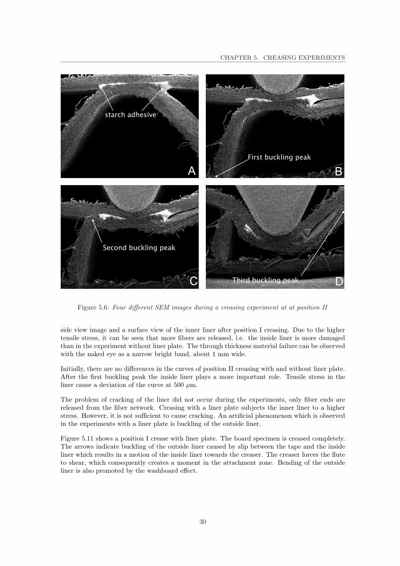
Figure 5.6: Four different SEM images during a creasing experiment at at position II
side view image and a surface view of the inner liner after position I creasing. Due to the highertensile stress, it can be seen that more fibers are released, i.e. the inside liner is more damagedthan in the experiment without liner plate. The through thickness material failure can be observedwith the naked eye as a narrow bright band, about 1 mm wide.
Initially, there are no differences in the curves of position II creasing with and without liner plate.After the first buckling peak the inside liner plays a more important role. Tensile stress in theliner cause a deviation of the curve at 500 µm.
The problem of cracking of the liner did not occur during the experiments, only fiber ends arereleased from the fiber network. Creasing with a liner plate subjects the inner liner to a higherstress. However, it is not sufficient to cause cracking. An artificial phenomenon which is observedin the experiments with a liner plate is buckling of the outside liner.
Figure 5.11 shows a position I crease with liner plate. The board specimen is creased completely.The arrows indicate buckling of the outside liner caused by slip between the tape and the insideliner which results in a motion of the inside liner towards the creaser. The creaser forces the fluteto shear, which consequently creates a moment in the attachment zone. Bending of the outsideliner is also promoted by the washboard effect.
30

CHAPTER 5. CREASING EXPERIMENTS
Figure 5.7: Four different SEM images during a creasing experiment at bat position III
31
CHAPTER 5. CREASING EXPERIMENTS
0 500 1000 1500 2000 25000
1000
2000
3000
load
[N/m
]
0 500 1000 1500 2000 25000
1000
2000
3000
load
[N/m
]
0 500 1000 1500 2000 25000
1000
2000
3000
displacement [µm]
load
[N/m
]
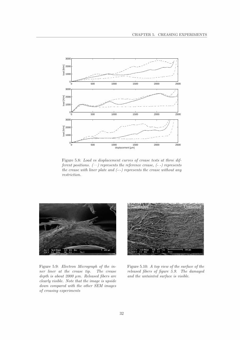
Figure 5.8: Load vs displacement curves of crease tests at three dif-ferent positions. (—) represents the reference crease, (- -) representsthe crease with liner plate and (-·-) represents the crease without anyrestriction.
Figure 5.9: Electron Micrograph of the in-ner liner at the crease tip. The creasedepth is about 2000 µm. Released fibers areclearly visible. Note that the image is upsidedown compared with the other SEM imagesof creasing experiments
Figure 5.10: A top view of the surface of thereleased fibers of figure 5.9. The damagedand the untainted surface is visible.
32

CHAPTER 5. CREASING EXPERIMENTS
Figure 5.11: A complete position I crease. Thearrows indicate buckling of the outside liner.
33

CHAPTER 5. CREASING EXPERIMENTS
34

Chapter 6
Confrontation of simulations vsexperiments
Finite element simulations are performed and compared with the experimental creasing tests inorder to investigate the ability of the model to capture the experimentally observed response.
6.1 Model definition
A close look at a piece of corrugated board shows that corrugated board has a non-symmetricalstructure and that the exact shape is not well defined. In Finite Element (FE) modelling thefluting is often approximated by a sine or a combination of arcs, [4] and [23]. In this study weadopt the sinusoidal shape. The so called washboard effect, i.e. non-flatness of the inner liner,is not included in the the models used initially. The influence of this effect is described furtherbelow.
The detailed FE model of a single wall corrugated board of type B is presented in figure 6.1. Theleft side is without the washboard effect, the right side includes this effect. The washboard effectis modelled as three arcs which are connected and is characterized by s, the amount of sagging ofthe liner. The flute period λ is 6.3 mm, the total height T is 3.0 mm, tl is 0.186 mm and tf is 0.155mm. The length on which the fluting and the liner are attached is represented by Λ = r, where ris the creaser tip radius; these connections are assumed to be rigid. The mechanical behaviour ofthe adhesive is not known and is neglected in this study. It is assumed that the drying procedurecauses no residual stress.
The corrugated board is modelled as a deformable body. The crease tip is modelled as a rigidcircular body with a radius of r=0.5 mm and undergoes a negative linear displacement, δ. Theanvil is also modelled as a rigid body and is constrained in each direction. The influence offriction is neglected. The down holders are placed 6.5 mm from the center line. The total modelis presented in figure 6.2.
The model assumes a plane strain state in CD direction, so ε22 = ε23 = ε12 = 0. Due tothis assumption the constants G12, G23, σ23y and σ12y do not influence the results. The fiberorientation is aligned with the elements as indicated in figure 6.1.
The simulation results presented in this chapter have all been obtained with the finite element
35

CHAPTER 6. CONFRONTATION OF SIMULATIONS VS EXPERIMENTS
Figure 6.1: Single wall corrugated board of type B. At the left side nowashboard effect is included. The right side includes the washboardeffect.
Figure 6.2: Loading and boundary conditions imposed on the finiteelement model
discretisation shown in figure 6.1. This discretisation has six linear quadrilateral elements acrossthe thickness. The total mesh consists of 11300 nodes and 9840. Refining the mesh did not resultin significant changes in the response, so that this mesh can be considered to be sufficiently fine.
6.2 Simulations with reference parameters
We will first present the results obtained with the reference material parameters as defined inchapter 5; the relevant reference parameters are recapitulated in table 6.1.
The simulated deformation of the board for the three creasing positions used in the experimentsare compared with images taken with an optical microscope, asumming that the influence ofdifferent ambient conditions (between optical and SEM) can be neglected. The model without thewashboard effect has been used for these simulations.
For each position, one representative experimental load-displacement curve has been plotted alongwith the corresponding simulation in figure 6.3. The important points in the figures are notedwith a roman character.
36

CHAPTER 6. CONFRONTATION OF SIMULATIONS VS EXPERIMENTS
0 500 1000 1500 2000 25000
1000
2000
3000
Load
[N/m
]
0 500 1000 1500 2000 25000
1000
2000
3000
Load
[N/m
]
0 500 1000 1500 2000 25000
1000
2000
3000
Displacement [µm]
Load
[N/m
]
A B
A B
A
B
position I
position II
position III
Figure 6.3: Experiments vs simulations at the three positions. (—)represent the experiments and (- -) represent the simulations
Table 6.1: Material parameters used in the reference simulationsParameter Value S.I. unit Parameter Value Unit
E1 3950 MPa G31 71 MPaE2 1650 MPa σ11y 13 MPaE3 20 MPa σ22y 4 MPaν12 0.65 - σ33y 4 MPaν31 0.0035 - σ31y 7.5 MPaν32 0.0055 -
Figures 6.4-6.6 show for each position the simulated and experimentally observed deformation atthe creaser displacements which have been marked in figure 6.3. The deformations predicted bythe FE model show a good agreement with the experiments. The stress in MD direction is alsodepicted in the deformation figures and will be discussed further below. Appendix C shows aoverview of creasing at the three positions. The results are discussed in more detail for each ofthe creaser positions below.
6.2.1 Position I
The top diagram in figure 6.3 shows the load-displacement curve at position I. The initial stiffnessfrom the simulation slightly deviates from the experiment. The experiment without down holdersalso show a lower initial stiffness. At (A) the flute collapses under the increasing stress, which isvisualized in figure 6.4.
In the experiments fixation of the flute between the inside and outside liner is observed. While thecreaser displacement proceeds the buckled flute unwinds itself along the inside and outside liner.Also delamination of the flute caused by the compressive load is observed. In the simulations, the
37

CHAPTER 6. CONFRONTATION OF SIMULATIONS VS EXPERIMENTS
Figure 6.4: Experimental vs simulation deformation at position I. σ11 is pre-sented in the numerical part of the image.
compressive load in the flute also initiates buckling. Once a buckle is initiated, however the flutethickness locally decreases and a plastic hinge is formed which can not unwind itself. As a result,the load continues to increase in the simulation, where it already decreases in the experiment.Delamination as encountered in the experiments weakens the flute compression stiffness. Sincethis is not included in the FE model an increase of creaser load is enforced.
Beyond point (B) the inside liner and fluting rotate around the plastic hinge, which preventsfixation and thus an increase of load. Fixation in position II is more important.
6.2.2 Position II
One can see a qualitative similarity between the experimental curve and the simulation curveof position II. In the simulation curve we can clearly distinguish the two buckling peaks of theexperimental curve which are associated with the two hinges that are formed in the flute (figure6.5. However, the buckling load is a factor two larger. The initial stiffness agree quite well, howevershortly after the start the simulated curve deviates for the experimental curve. The first bucklingpeak is reached after a displacement of 400 µm in the simulation whereas it occurs already atapproximately 150 µm in the experiment.
Next, the load increases and another buckle initiates which results in a decrease of load. Beyond(A) the creaser reaction force increases. Fixation of the flute is shown in figure 6.5 image B, seealso the displacement of the buckle in the experiment.
38
CHAPTER 6. CONFRONTATION OF SIMULATIONS VS EXPERIMENTS
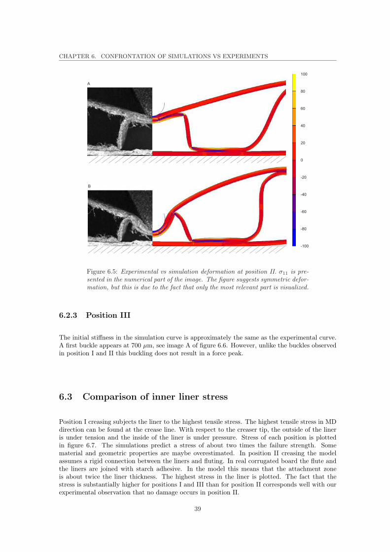
Figure 6.5: Experimental vs simulation deformation at position II. σ11 is pre-sented in the numerical part of the image. The figure suggests symmetric defor-mation, but this is due to the fact that only the most relevant part is visualized.
6.2.3 Position III
The initial stiffness in the simulation curve is approximately the same as the experimental curve.A first buckle appears at 700 µm, see image A of figure 6.6. However, unlike the buckles observedin position I and II this buckling does not result in a force peak.
6.3 Comparison of inner liner stress
Position I creasing subjects the liner to the highest tensile stress. The highest tensile stress in MDdirection can be found at the crease line. With respect to the creaser tip, the outside of the lineris under tension and the inside of the liner is under pressure. Stress of each position is plottedin figure 6.7. The simulations predict a stress of about two times the failure strength. Somematerial and geometric properties are maybe overestimated. In position II creasing the modelassumes a rigid connection between the liners and fluting. In real corrugated board the flute andthe liners are joined with starch adhesive. In the model this means that the attachment zoneis about twice the liner thickness. The highest stress in the liner is plotted. The fact that thestress is substantially higher for positions I and III than for position II corresponds well with ourexperimental observation that no damage occurs in position II.
39

CHAPTER 6. CONFRONTATION OF SIMULATIONS VS EXPERIMENTS
Figure 6.6: Experimental vs simulation deformation at position III. σ11 ispresented in the numerical part of the image.
6.4 Influence of material and geometric properties
The differences between the experiments and the simulations are in some cases quite large. Someparameters may have been overestimated. This section describes the influence and sensitivity ofthe known and unknown material parameters. This will help us to determine the governing set ofparameters of the crease process.
For this investigation the crease simulations are performed at position II. Cracking of the liner ismainly governed by the flute stiffness. The flute stiffness is best tested at this position. To reducecpu time the analysis is assumed to be symmetric with respect to the creaser displacement path.
6.4.1 Material properties
In our model orthotropic elasto-plasticity is assumed. Figure 6.8 shows the difference betweenisotropic elasto-plasticity and orthotropic elasto-plasticity. The used parameters are presentedin table 6.2. In case of isotropic elastic behaviour the initial structural stiffness is higher. Onlyone buckling peak can be noticed in the resulting curve. The rapid increase of load beyond 1200µm observed in the reference computation does not occur in case of isotropic elastic behaviour.No noticeable thickness reduction of the flute at the buckle zone is observed. No fixation of theflute between the liners occurs and while the creaser moves downward the fluting unwinds itselfalong the liners. There is little difference between ISO-ISO and ISO-ORTHO curves, but a largedifference with the reference curve, so the elastic parameters are important for the overall response,even in the plastic regime. Large plastic strains mainly occur in the fluting in the buckle zones.
40

CHAPTER 6. CONFRONTATION OF SIMULATIONS VS EXPERIMENTS
0 500 1000 1500 2000 2500−20
0
20
40
60
80
100
120
Displacement [µm]
σ 11 [M
Pa]
position I
position III
position II
0 500 1000 1500 20000
500
1000
1500
2000
2500
3000
3500
4000
Displacement [µm]
Load
[N/m
]
iso−iso
iso−ortho
reference
exp
Figure 6.7: The highest stress (σ11) of eachposition at the crease line at the bottom ofthe inside liner
Figure 6.8: Load-displacement curve ofisotropic and orthotropic elasto-plasticity;see table 6.2 for material data used.
Table 6.2: Parameters used for different material modelsmodel abbreviation parameters
isotropic elasto-plasticity iso-iso E = E1, ν = 0.33, Rii = 1, Rij = 1isotropic elasticity, orthotropic plasticity iso-ortho R11 = 1, R22 = R33 = 0.30, Rij = 1
orthotropic elasto-plasticity reference reference parameters
In the reference set there is a factor of 200 between E1 and E3 and a factor of 20 between theisotropic G31 (about 1400 MPa) and orthotropic G31. Simulations with an unrealistic E3 = E1
(the other parameters equal the reference parameters) exhibit a qualitatively similar shape asthe ISO-ISO case, yet at a somewhat lower reaction force. A simulation with an unrealisticG31 = 1400 MPa shows a qualitatively similar curve as the reference curve. The shape of theload-displacement curve is mainly governed by the buckling behaviour of the flute, which in turndepends predominantly on the out-of-plane elastic modulus E3.
Shortly after the start of the simulation curve the initial stiffness deviates from the experiments.This can be corrected by taking for G31 = 34 which can be found in literature [22]. This valueis about a factor of two lower than the shear modulus of the reference parameters. In figure 6.9these curve are presented. A more accurate stiffness is obtained with the lower shear modulus.Variations in shear stress mainly affect the flute when it is deformed.
As described in chapter 4 the out-of-plane Poission’s ratios ν are close to zero (ν31 = 0.0035 andν32 = 0.0055). Let us assume ν in thickness direction is zero. The result is also presented infigure 6.9. Little difference can be noticed in the curve. Thus the out-of-plane ν has no significantinfluence on the response.
Due to the incompressibility of the Hill48 yield criterion the yield stress is symmetric in tensionand compression. Since the fluting is mainly in compression, the yield stress is overestimated. [3]suggested to multiply the reference yield stress with 0.65 to approximate the compressive yieldstress. Figure 6.10 presents the curve with the adjusted reference yield stress, σref = 8.5 MPa, forthe flute only. Again a better initial stiffness and lower overall load is obtained. The first bucklingpeak is reached earlier.
As described before, in the reference simulation a first approximation of R31 = 1 is used, so
41

CHAPTER 6. CONFRONTATION OF SIMULATIONS VS EXPERIMENTS
0 500 1000 1500 20000
500
1000
1500
2000
2500
3000
3500
4000
Displacement [µm]
Load
[N/m
]
reference
G31
=35
ν32
=ν31
=0
exp
0 500 1000 1500 20000
500
1000
1500
2000
2500
3000
3500
4000
Displacement [µm]
Load
[N/m
]
exp
reference σ
ref=8.5
Figure 6.9: Variation of G31 and ν31 =ν32 = 0
Figure 6.10: Variation of reference yieldstress
σ31y = 7.5 MPa. In chapter 4 a typical shear yield stress of 1 MPa is stated. The obtained curveis presented in figure 6.11. Shortly after the start the curve deviates from the experimental curve.Only the first buckling peak is observed.
0 500 1000 1500 20000
500
1000
1500
2000
2500
3000
3500
4000
Displacement [µm]
Load
[N/m
] reference
exp σ
31y=1
0 500 1000 1500 20000
500
1000
1500
2000
2500
3000
3500
4000
Displacement [µm]
Load
[N/m
]
exp
reference washboard effect
Λ=0
Figure 6.11: Influence of shear yield stress Figure 6.12: Simulations with different ge-ometry compared with the experiments at po-sition II
6.4.2 Geometric properties
First the washboard effect is added to the model. The washboard effect decreases the first peakin the load-displacement response, see figure 6.12. The initial stiffness is not influenced by thewashboard effect. Initially, there is little resistance from the inside liner to the crushing of theflute. In fact, the washboard liner is longer than a straight liner. When the liner is fully stretchedthe liner starts to play a role, i.e. in the second peak. The length difference of the liner results ina postponed as well as a higher second peak.
The attachment length Λ is hard to measure, it differs along the board and the mechanical be-haviour of the adhesive is unknown. If it is set to Λ = 0 no noticeable first peak is obtained (figure6.12) and the initial stiffness is closer to the experimental value. The effect on the remainder ofthe load-displacement curve is similar to that of a longer inner liner: the second peak is again
42
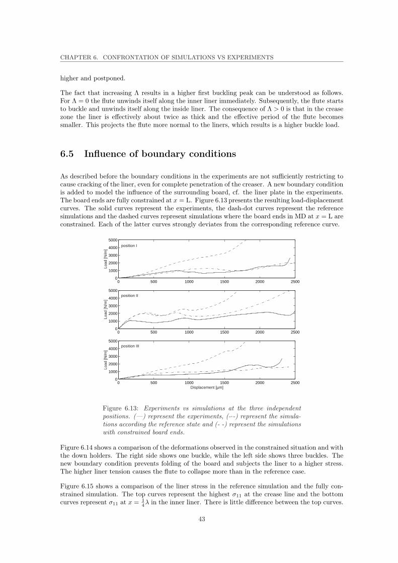
CHAPTER 6. CONFRONTATION OF SIMULATIONS VS EXPERIMENTS
higher and postponed.
The fact that increasing Λ results in a higher first buckling peak can be understood as follows.For Λ = 0 the flute unwinds itself along the inner liner immediately. Subsequently, the flute startsto buckle and unwinds itself along the inside liner. The consequence of Λ > 0 is that in the creasezone the liner is effectively about twice as thick and the effective period of the flute becomessmaller. This projects the flute more normal to the liners, which results is a higher buckle load.
6.5 Influence of boundary conditions
As described before the boundary conditions in the experiments are not sufficiently restricting tocause cracking of the liner, even for complete penetration of the creaser. A new boundary conditionis added to model the influence of the surrounding board, cf. the liner plate in the experiments.The board ends are fully constrained at x = L. Figure 6.13 presents the resulting load-displacementcurves. The solid curves represent the experiments, the dash-dot curves represent the referencesimulations and the dashed curves represent simulations where the board ends in MD at x = L areconstrained. Each of the latter curves strongly deviates from the corresponding reference curve.
0 500 1000 1500 2000 25000
1000
2000
3000
4000
5000
Load
[N/m
]
0 500 1000 1500 2000 25000
1000
2000
3000
4000
5000
Load
[N/m
]
0 500 1000 1500 2000 25000
1000
2000
3000
4000
5000
Displacement [µm]
Load
[N/m
]
position I
position II
position III
Figure 6.13: Experiments vs simulations at the three independentpositions. (—) represent the experiments, (-·-) represent the simula-tions according the reference state and (- -) represent the simulationswith constrained board ends.
Figure 6.14 shows a comparison of the deformations observed in the constrained situation and withthe down holders. The right side shows one buckle, while the left side shows three buckles. Thenew boundary condition prevents folding of the board and subjects the liner to a higher stress.The higher liner tension causes the flute to collapse more than in the reference case.
Figure 6.15 shows a comparison of the liner stress in the reference simulation and the fully con-strained simulation. The top curves represent the highest σ11 at the crease line and the bottomcurves represent σ11 at x = 1
4λ in the inner liner. There is little difference between the top curves.
43

CHAPTER 6. CONFRONTATION OF SIMULATIONS VS EXPERIMENTS
Figure 6.14: Deformation for constrained edge (left) and reference situationusing down holders (right) at position I
The stress here is mainly governed by bending of the inside liner. The sudden change in thedashed curve at 2000 µm is caused by the initiation of the second and third buckle in the flute.The bottom curves clearly show that the inside liner is subjected to a much higher stress in caseof the new boundary conditions. This corresponds well with the observation in the experimentsthat the more constrained configuration (using the liner plate) results in more damage.
0 500 1000 1500 2000 25000
20
40
60
80
100
120
Displacement [µm]
σ 11 [M
Pa]
at crease line (x=0)
at x=1/4 λ
Figure 6.15: Comparison of the highest stress atthe crease line for position I creasing. (—) rep-resents the reference simulation and (- -) repre-sents real-life creasing. The top curves representthe highest σ11 at the crease line and the bottomcurves represent σ11 at x = 1
4λ in the inner liner.
6.6 Summary of observations
The previous investigation of the material and geometric properties and boundary conditions canbe recapitulated as follows
• The deformations predicted by the finite element (FE) model show a qualitative good agree-ment with the experiments. However, a quantitative agreement cannot be given. The loadresponse deviates about max. a factor of two.
• Plasticity mainly occurs in the buckle zones. The buckles act as plastic hinges and can-not move. The low stiffness in thickness direction causes the buckling peaks. The lack ofcompressibility of the Hill48 yield criterion overestimates the stiffness.
44

CHAPTER 6. CONFRONTATION OF SIMULATIONS VS EXPERIMENTS
• Out-of-plane Poisson’s ratios have no significant influence on the load-displacement curve.
• The out-of-plane shear elastic and plastic parameters influence the load response.
• The attachment length influences the first buckling peak.
• The washboard effect has a positive effect on preventing cracking of the liner.
• Real-life creasing subjects the inside liner to a higher stress.
45

CHAPTER 6. CONFRONTATION OF SIMULATIONS VS EXPERIMENTS
46

Chapter 7
Conclusion and recommendations
The creasing behaviour of corrugated board has been studied by a combined experimental-numericalapproach. The crease simulations show a good qualitative agreement with the observed exper-imental deformation, buckling and load response. However, the quantitative agreement is lesssatisfactory. Difference in load of max. 100 % is encountered. This is caused by the lack ofcompressibility of the Hill yield criterion, the out-of-plane elastic and plastic components and de-lamination of the flute, which have a significant influence. The flute stiffness plays an importantrole in the deviation. A constitutive model which allows to model compressibility and delamina-tion should be applied and a method to determine the out-of-plane shear modulus and shear yieldstress has to be developed.
The present finite element model assumes a rigid connection between the flute and the liner. Thelength of this connection has a significant influence on the load response. Peel tests should becarried out in order to get insight in the strength of the joining of the liner and the flute andwhether the assumption of the connection being rigid is sufficient.
Cracking of the inside liner is not observed during the experiments, only some damage of the lineris encountered. If new boundary conditions which take the influence of the surrounding boardinto account are applied, the inner liner is subjected to a higher tensile stress. Experiments andsimulations confirm this. A new tool should be made which constrains the board ends. One wayto achieve this is to inject a hardening substance between the liners at the board ends, whichmakes it possible to clamp the ends.
An observation which may be of interest for the industrial practice is that the cracked board sheets(unfolded boxes including creases and cuts) provided by Kappa Containerboard exhibit crackingpredominantly near cuts. The cut ends are points where stress concentrates and which may causecracking. Cutter/creaser designs which avoid these concentrations, e.g. by punching a corner relief(a circular hole at the transition from a cut to a crease), may give rise to less cracking. A cornerrelief is often applied in sheet metal applications. In terms of further research, the influence ofa cut should be investigated, which implies that a two dimensional model is not sufficient and athree dimensional model must be developed.
47

CHAPTER 7. CONCLUSION AND RECOMMENDATIONS
48

Bibliography
[1] Allansson, A., (2001) Stability and collapse of corrugated board; Numerical and ExperimentalAnalysis, Structural Mechanics LTH, Sweden
[2] Bergen van, W.J.C., (1990) Het papierboek, Stam Technische Boeken, Culemborg (in Dutch)
[3] Beldie, L., (2001) Mechanics of paperboard packages, performance at short term static loading,Div. of Structural Mechanics, Lund university
[4] Biancolini, M. E., (2005) Evaluation of equivalent stiffness properties of corrugated board,Composite Structures 69 (3)
[5] Brekelmans, W.A.M., (2002) Mechanical Characterisation of Materials: Constitutive Mod-elling, dictaat 4797, TU/e Eindhoven
[6] Castro, J., Ostoja-Starzewski, M., (2003) Elasto-plasticity of paper, International Journal ofPlasticity, Volume 19, Issue 12, December 2003, Pages 2083-2098
[7] Dekker, J.C., Rilbaarheid, Rapport 2A, PRONTA, periode 1 oktober 1995 tot 1 januari 1996,15 januari 1996, ATO-DLO, Wageningen (in Dutch)
[8] Dekker, J.C., Rilbaarheid, Rapport 2B, PRONTA, periode 1 januari 1996 tot 1 juli 1996, 30juli 1996 ATO-DLO, Wageningen (in Dutch)
[9] Dekker, J.C., Rilbaarheid, Rapport 2C, PRONTA, periode 1 juli 1996 tot 1 januari 1997, 7april 1997 ATO-DLO, Wageningen (in Dutch)
[10] D828-97(2002) Standard Test Method for Tensile Properties of Paper and Paperboard UsingConstant-Rate-of-Elongation Apparatus, ASTM International
[11] Hill, R. (1950) The mathematical theory of plasticity, Oxford University Press, London
[12] Hill, R., Constitutive Modelling of Orthotropic Plasticity in Sheet Metals, J. Mech. Phys.Solids, 38 (1990), pp. 405-417.
[13] http://www4.ncsu.edu/ hubbe/FIBR.htm
[14] Mäkelä, P., Östlund, S., (2003) Orthotropic elasticŰplastic material model for paper materials,International Journal of Solids and Structures, Volume 40, Issue 21, October 2003, Pages5599-5620
[15] Meinders T., (2000) Developments in numerical simulations of the real life deep drawingprocess, Ph.D. Thesis , University of Twente, Enschede
[16] Nagasawa, S. (2003) Effect of crease depth and crease deviation on folding deformation char-acteristics of coated paperboard, Journal of Materials Processing Technology, Volume 140,Issues 1-3, 22 September 2003, Pages 157-162
49

BIBLIOGRAPHY
[17] Netz, E., (1998) Washboarding and print quality of corrugated board, Packaging Technologyand Science Volume 11, Issue 4, 1998. Pages 145-167
[18] Niskanen, K. (1998) Paper and paperboard converting, Fapet Oy, Helsinki
[19] Niskanen, K. (1998) Paper physics, Fapet Oy, Helsinki
[20] Scott, William E. (1995) Properties of paper, an introduction, TAPPI PRESS, Atlanta
[21] Stenberg, N., (2003) A model for the throug-thickness elastic-plastic behaviour of paper, In-ternational Journal of Solids and Structures 40, 7483-7498.
[22] Stenberg, N., Fellers C., Östlund, S. (2003) Plasticity in the thickness direction of paperboardunder combined shear and normal loading, Journal of Engineering Materials and Technology123(4) 184-190.
[23] Urbanik, T.J., (2001) Effect of Corrugated Flute Shape on Fibreboard Edgewise Crush Strengthand Bending Stiffness, J. Pulp and Pap. Sci. 27(10): 330-335.
[24] Xia, Q.S., Boyce, M.C., Parks, D.M., (2002) A constitutive model for the anisotropic elasticŰ-plastic deformation of paper and paperboard, International Journal of Solids and Structures39, 4053Ű4071.
[25] Xia, Q.S., (2002) Mechanics of inelastic deformation and delamination in paperboard, MIT-THESES:2002-381
[26] Xue, Z., Hutchinson, J.W., 2004. Constitutive model for quasi-static deformation of metallicsandwich cores, International Journal for Numerical Methods in Engineering. 61, 2205-2238.
50

Appendices
51


Appendix A
Hill48 detailed calculations
Hill48 in MSC.MARC/MENTAT 2005
The Hill48 yield function as provided in MSC.MARC/MENTAT 2005 reads
f =12[a1(σ22 − σ33)2 + a2(σ33 − σ11)2 +
a3(σ11 − σ22)2 + 6a4σ223 + 6a5σ
231 + 6a6σ
212
]− σ2ref (A.1)
The constants a1, a2, a3, a4, a5 and a6 are
a1 =1
R222
+1
R233
− 1R2
11
; a4 =1
R223
a2 =1
R211
+1
R233
− 1R2
22
; a5 =1
R231
(A.2)
a3 =1
R211
+1
R222
− 1R2
33
; a6 =1
R212
Limitation of orthotropy
Hill48 impedes a high degree of orthotropy in three directions. The constants must obey
FG + GH + HF > 0 (A.3)
Substituting
2F =1
σ222y
+1
σ233y
− 1σ2
11y
2G =1
σ211y
+1
σ233y
− 1σ2
22y
(A.4)
2H =1
σ211y
+1
σ222y
− 1σ2
33y
in equation (A.3) and rewriting it in terms of Rii with R11 = 1, results in
−(
1R2
33
)2
+ 2(
1 +1
R222
)1
R233
−(
1− 1R2
22
)2
> 0 (A.5)
53
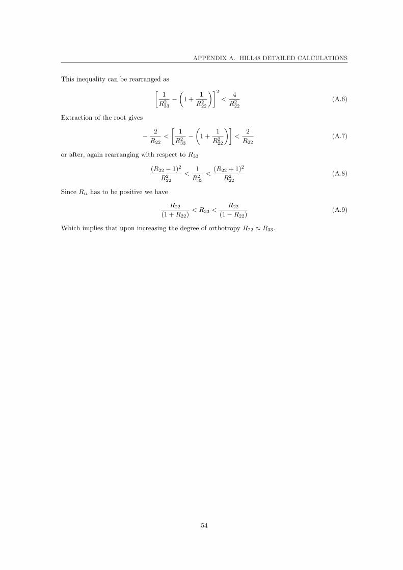
APPENDIX A. HILL48 DETAILED CALCULATIONS
This inequality can be rearranged as[
1R2
33
−(
1 +1
R222
)]2
<4
R222
(A.6)
Extraction of the root gives
− 2R22
<
[1
R233
−(
1 +1
R222
)]<
2R22
(A.7)
or after, again rearranging with respect to R33
(R22 − 1)2
R222
<1
R233
<(R22 + 1)2
R222
(A.8)
Since Rii has to be positive we have
R22
(1 + R22)< R33 <
R22
(1−R22)(A.9)
Which implies that upon increasing the degree of orthotropy R22 ≈ R33.
54

Appendix B
Calculation of in-plane shear
Shear modulus
With the use of elasticity theory, the assumption of plane stress and knowing E1, E2 and ν12 itis possible to extract G12 from the tensile test at 45o. The plane stress matrix representation ofHooke’s law is
ε˜ = Sσ˜ (B.1)
with
σ˜ =
σ11
σ22
σ12
ε˜ =
ε11
ε22
2ε12
S =
E−11 −ν21E
−12 0
−ν12E−11 E−1
2 00 0 G−1
12
(B.2)
The stress tensor σ is
σ =12σ(~e1 + ~e2)(~e1 + ~e2)
=12σ(~e1~e1 + ~e1~e2 + ~e2~e1 + ~e2~e2) (B.3)
where σ denotes the axial stress in loading direction. The normal strain ε of the strain tensorε = ε11~e1~e1 + ε12
(~e1~e2 + ~e2~e1
)+ ε22~e2~e2 along the normal vector ~n is determined as
ε = ~n · ε · ~n with ~n =1√2(~e1 + ~e2) (B.4)
Using (B.1, the normal strain can be expressed in terms of the stress components as
ε =12
(~e1 + ~e2
)·(ε11~e1~e1 + ε12
(~e1~e2 + ~e2~e1
)+ ε22~e2~e2
)·(~e1 + ~e2
)
=12
(ε11 + ε22 + 2ε12
)(B.5)
=12
(1
E1− ν21
E2+
1E2
− ν12
E1+
1G12
)12σ
=14
(1− ν12
E1+
1− ν21
E2+
1G12
)σ
The initial slope of the tensile test under 45o with respect to the machine direction in figure 4.5should thus equal the inverse of the compliance given by (B.5). Since E1, E2, ν12 and ν21 areknown, G12 can be determined from this relation.
55

APPENDIX B. CALCULATION OF IN-PLANE SHEAR
In-plane shear yield stress
The constant N can be determined from the tensile test of a specimen at 45o if only σ33y is known.For a plane stress state the yield criterion (3.15) reduces to
(G + H)σ211 − 2Hσ11σ22 + (F + H)σ2
22 + 2Nσ212 = 1 (B.6)
The previous section showed that σ11 = σ22 = σ12 = 12σ. At yield we have σ45y and equation
(B.6) thus further reduces to
14(F + G)σ2
45y +12Nσ2
45y = 1 (B.7)
(F + G) can be derived from a biaxial tensile test, σ11 = σ22 = σ. Note that (F + G)−1/2 is alsothe yield stress in thickness direction, see equation (3.17). Finally, N can be derived from
2N = 4σ−245y − (F + G) (B.8)
56

Appendix C
Crease simulations overview
Figure C.1: Creasing at different positions
57

APPENDIX C. CREASE SIMULATIONS OVERVIEW
58

Dankwoord
Bij deze wil ik graag iedereen bedanken voor de hulp tijdens en bij mijn afstuderen. Mijn oudersdie de eerste (en laatste) docenten zijn waar ik ooit onderricht van heb genoten en hun steun opeen diversiteit aan vlakken tijdens mijn leven en tijdens deze en vorige opleidingen.
Op het professioneel technische vlak wil ik graag mijn begeleider, Ron Peerlings, bedanken voorzijn begeleiding, hulp, correcties en tijd. Ook wil ik Marc van Maris bedanken voor zijn praktischeinput tijdens de experimenten.
Verder wil ik, ondanks de lange productietijd, de gemeenschappelijke technische dienst (GTD)bedanken voor het vervaardigen van de benodigde gereedschappen.
Ook mijn mede VKO-ers wil ik bedanken voor de gezellige momenten die ik de afgelopen tijd methen heb mogen beleven.
De TU/e heeft mij mijn basiskennis aanzienlijk verbreed voor de rest van mijn (werkzame) leven,doch was het niet de Britse natuurkundige Sir Isaac Newton die zei:
"Wat wij weten is een druppel, wat wij niet weten een oceaan."
Na de studies in mijn leven kan ik mijzelf niet geheel onttrekken aan het idee dat ik de wijsheidnog niet in pacht heb. Het gevoel dat mijn educatie nog lang niet ten einde is overheerst sterk.Desalniettemin is een spreekwoordelijke mijlpaal bereikt.
59