crc report no. e-123
TRANSCRIPT

COORDINATING RESEARCH COUNCIL INC 5755 NORTH POINT PARKWAY SUITE 265 ALPHARETTA GA 30022
CRC Report No E-123
ON-ROAD REMOTE SENSING OF AUTOMOBILE EMISSIONS IN THE
TULSA AREA FALL 2019
April 2020
The Coordinating Research Council Inc (CRC) is a non-profit
corporation supported by the petroleum and automotive
equipment industries CRC operates through the committees
made up of technical experts from industry and government
who voluntarily participate The four main areas of research
within CRC are air pollution (atmospheric and engineering
studies) aviation fuels lubricants and equipment
performance heavy-duty vehicle fuels lubricants and
equipment performance (eg diesel trucks) and light-duty
vehicle fuels lubricants and equipment performance (eg
passenger cars) CRCrsquos function is to provide the mechanism
for joint research conducted by the two industries that will
help in determining the optimum combination of petroleum
products and automotive equipment CRCrsquos work is limited to
research that is mutually beneficial to the two industries
involved The final results of the research conducted by or
under the auspices of CRC are available to the public
CRC makes no warranty expressed or implied on the
application of information contained in this report In
formulating and approving reports the appropriate committee
of the Coordinating Research Council Inc has not
investigated or considered patents which may apply to the
subject matter Prospective users of the report are responsible
for protecting themselves against liability for infringement of
patents
On-Road Remote Sensing of Automobile
Emissions in the Tulsa Area Fall 2019
Gary A Bishop
Department of Chemistry and Biochemistry
University of Denver
Denver CO 80208
April 2020
On-Road Remote Sensing in the Tulsa Area Fall 2019 3
EXECUTIVE SUMMARY
The University of Denver conducted a five-day remote sensing study in the Tulsa Oklahoma
area in September of 2019 The remote sensor used in this study measures the molar ratios of
CO HC NO SO2 NH3 and NO2 to CO2 in motor vehicle exhaust From these ratios we
calculate the percent concentrations of CO CO2 HC NO SO2 NH3 and NO2 in the exhaust that
would be observed by a tailpipe probe corrected for water and any excess oxygen not involved
in combustion Mass emissions per mass or volume of fuel can also be determined and are
generally the preferred units for analysis The system used in this study was configured to
determine the speed and acceleration of the vehicle and was accompanied by a video system to
record the license plate of the vehicle and from this record the vehiclersquos model year Since fuel
sulfur has been nearly eliminated in US fuels SO2 emissions have followed suit and while we
collected vehicle SO2 measurements we did not calibrate those readings and they are not
included in the discussion of the results
Five days of fieldwork September 9 ndash 13 2019 were conducted on the uphill interchange ramp
from westbound US64 (Broken Arrow Expressway) to southbound US169 This is the same
location previously used for measurements in the fall of 2003 2005 2013 2015 and 2017 A
database was compiled containing 23376 records for which the State of Oklahoma and the
Cherokee Nation provided registration information All of these records contained valid
measurements for at least CO and CO2 and most records contained valid measurements for the
other species as well The database as well as others compiled by the University of Denver can
be found online at wwwfeatbiochemduedu
The 2019 mean CO HC NO NH3 and NO2 emissions for the fleet measured in this study were
116 gCOkg of fuel (009) 19 gHCkg of fuel (69 ppm) 11 gNOkg of fuel (76 ppm) 034
gNH3kg of fuel (42 ppm) and 002 gkg of fuel (1 ppm) respectively When compared with
previous measurements from 2017 we find that mean CO (+5) and HC (+12) emissions
slightly increased though the differences are not statistically significant NO and NH3 emissions
in 2019 show statistically significant reductions when compared with the 2017 data with mean
NO emissions decreasing by 21 and NH3 emissions by 8 Figure ES1 shows the mean fuel
specific emissions for CO ( left axis) HC ( right axis) and NO ( right axis) versus
measurement year for all the data sets collected at the Tulsa site Uncertainties are standard error
of the mean calculated using the daily means Since 2003 the fuel specific CO emissions have
decreased by 66 HC by 41 and NO by 70 As seen in the plot the largest absolute
reductions occurred between the 2005 and 2013 measurements
The average Tulsa fleet age again increased by 01 years (20119) which is approximately 81
years old Fleet mean emissions are still dominated by a few high emitting vehicles and for the
2019 data set the highest emitting 1 of the measurements (99th
percentile) is responsible for
30 32 35 16 and 100 of the CO HC NO NH3 and NO2 emissions respectively
The Tulsa site was one of the first in which the University of Denver collected NH3 emissions
from light-duty vehicles in 2005 and now has one of the longest running NH3 measurement
On-Road Remote Sensing in the Tulsa Area Fall 2019 3
trends With this measurement campaign we have now collected 5 data sets with fuel specific
NH3 emissions and the means and standard error of the mean uncertainties are listed in Table
ES1
Ammonia emissions have experienced an overall 32 reduction in emissions over these fourteen
years (-12 year over year change) Figure ES2 compares the five Tulsa data sets versus vehicle
age where year 0 vehicles are 2020 2018 2016 2014 and 2006 models for the 2019 2017
2015 2013 and 2005 data sets The uncertainties plotted are standard error of the mean
calculated from distributing the daily means for each age groups data The lower rate of increase
in NH3 emissions as a function of vehicle age seen initially with the 2013 data set is still a
feature of the 2019 data Tier 3 vehicles phased into the vehicle fleet with the 2017 model year
and these vehicles appear to continue the trend of lower NH3 emissions in the 1 to 4 year old
Figure ES1 Tulsa area historical fuel specific fleet mean emissions for CO ( left axis) HC ( right
axis) and NO ( right axis) by measurement year Uncertainties are standard error of the mean
calculated using the daily measurements The fuel specific HC means have been adjusted as described in
the report
40
30
20
10
00
gH
C o
r gN
Ok
g o
f Fu
el
201820152012200920062003
Measurement Year
40
30
20
10
0
gC
Ok
g o
f F
uel
CO
HC (adjusted)
NO
Table ES1 Mean Fuel Specific Ammonia Emissions with Standard Error of the Mean
Uncertainties for the Five Tulsa Measurement Campaigns
Measurement Year Mean gNH3kg of Fuel
2005 05 plusmn 001
2013 043 plusmn 001
2015 037 plusmn 0001
2017 037 plusmn 0005
2019 034 plusmn 001
On-Road Remote Sensing in the Tulsa Area Fall 2019 4
vehicles For example NH3 emissions of one year old vehicles have declined by 47 (023 to
012 gNH3kg of fuel) since 2013 The location of the peak NH3 emissions is not possible to
definitively assign in the current data set but it has certainly been pushed beyond the 20 year
mark for an estimated 3-way catalyst lifetime
Over the same fourteen year period NO emissions have decreased by 62 (29 gNOkg of fuel in
2005 to 11 gNOkg of fuel in 2019) almost twice the decreases observed for NH3 It is not
understood why NO emissions have decreased more during this fourteen year period than NH3
since they have a common origination point in engine out NO emissions With the disparity in
these reductions NH3 is now the dominate reactive nitrogen compound emitted at the tailpipe
We again investigated potential differences between vehicles registered with the Cherokee
Nation and those registered in the State of Oklahoma The Cherokee Nation fleet observed at this
location is smaller making up only 68 of the overall matched plates but is more than a year
newer (mean model year of 20131 versus 20118) Because of its age the Cherokee Nation fleet
has lower mean emission for all of the species measured however they are accompanied with
larger uncertainties When the Oklahoma plated vehicles are age adjusted to match the age
distribution of the Cherokee Nation fleet the Oklahoma fleet turns out to have lower or similar
emissions for every species but NO and NH3
Figure ES2 Mean gNH3kg emissions plotted against vehicle age for the 2019 2017 2015 2013 and
2005 measurements at the Tulsa site The uncertainty bars plotted are the standard error of the mean
determined from the daily samples
12
10
08
06
04
02
00
gN
H3k
g o
f F
uel
2520151050
Vehicle Age
2005
201320152017
2019
On-Road Remote Sensing in the Tulsa Area Fall 2019 5
INTRODUCTION
Since the early 1970rsquos many heavily populated cities in the United States have violated the
National Air Quality Standards (NAAQS) that have been established by the Environmental
Protection Agency (EPA) pursuant to the requirements of the Federal Clean Air Act1 2
Carbon
monoxide (CO) levels become elevated primarily due to direct emission of the gas Ground-level
ozone a major component of urban smog is produced by the photochemical reaction of nitrogen
oxides (NOx) and hydrocarbons (HC) Ambient levels of particulate emissions can result either
from direct emissions of particles or semi-volatile species or from secondary reactions between
gaseous species such as ammonia and nitrogen dioxide (NO2) As of 2015 on-road vehicles
continued to be estimated as one of the larger sources for major atmospheric pollutants
contributing approximately 39 of the CO 14 of the volatile organic carbons 3 of the
ammonia (NH3) and 36 of the NOx to the national emission inventory3
The use of the internal combustion engine and the combustion of carbon based fuels as one of
our primary means of transportation accounts for it being a significant contributor of species
covered by the NAAQS For a description of the internal combustion engine and causes of
pollutants in the exhaust see Heywood4 Properly operating modern vehicles with three-way
catalysts are capable of partially (or completely) converting engine-out CO hydrocarbons (HC)
and nitric oxide (NO) emissions to carbon dioxide (CO2) water and nitrogen Control measures
to decrease mobile source emissions in non-attainment areas include inspection and maintenance
(IM) programs reformulated and oxygenated fuel mandates and transportation control
measures but the effectiveness of these measures are difficult to quantify Many areas remain in
non-attainment for ozone The further tightening of the federal eight-hour ozone standards (first
introduced by the EPA in 1997 subsequently lowered in 2008 and again in 2015) means that
many new locations are likely to have difficulty meeting the standards in the future5
Beginning in 1997 the University of Denver began conducting on-road tailpipe emission surveys
at selected sites to follow long-term vehicle emission trends A site northwest of Chicago IL in
Arlington Heights was the first to be established but over the years we have also collected
measurements in Los Angeles CA Denver CO Omaha NE Phoenix AZ Riverside CA and
Tulsa OK6 Following a protocol established by the Coordinating Research Council (CRC) as
part of the E-23 program the data collected have provided valuable information about the
changes in fleet average on-road emission levels and the data have been used by many
researchers to establish fleet emission trends and inventories7-13
Reflecting a desire to continue evaluating the historical and recent emissions trends several of
the previous E-23 sites were chosen for additional data collection in 2013 As part of the E-106
program two additional measurement campaigns were conducted in Tulsa OK in 2013 and 2015
CRC E-123 continues these measurements and this report describes the on-road emission
measurements collected in Tulsa OK area in the fall of 2019 Measurements were made on five
consecutive weekdays from Monday September 9 to Friday September 13 between the hours
of 700 and 1900 on the uphill interchange ramp from westbound US64 (Broken Arrow
Expressway) to southbound US169
On-Road Remote Sensing in the Tulsa Area Fall 2019 6
The Tulsa area was originally selected as a location to study vehicle emissions because it is one
of the larger metropolitan areas in the US that has never been required to have a vehicle
Inspection amp Maintenance program (IM) Tulsa is also geographically isolated from cities that
do have IM programs which helps to limit importation of IM failing vehicles For this reason a
program to conduct remote sensing emission measurements in Tulsa can provide a useful
baseline for comparison with similar data collected from other cities
MATERIALS AND METHODS
The FEAT remote sensor used in this study was developed at the University of Denver for
measuring the pollutants in motor vehicle exhaust and has previously been described in the
literature14-16
The instrument consists of a non-dispersive infrared (NDIR) component for
detecting CO CO2 and HC and twin dispersive ultraviolet (UV) spectrometers for measuring
oxides of nitrogen (NO and NO2) SO2 and NH3 (026 nmdiode resolution) The source and
detector units are positioned on opposite sides of the road in a bi-static arrangement Collinear
beams of infrared (IR) and UV light are passed across the roadway into the IR detection unit and
are then focused through a dichroic beam splitter which serves to separate the beams into their
IR and UV components The IR light is then passed onto a spinning polygon mirror which
spreads the light across the four infrared detectors CO CO2 HC and reference
The UV light is reflected from the surface of the dichroic mirror and is focused onto the end of a
quartz fiber bundle that is mounted to a coaxial connector on the side of the detector unit The
quartz fiber bundle is divided in half to carry the UV signal to two separate spectrometers The
first spectrometer was adapted to expand its UV range down to 200nm in order to measure the
peaks from SO2 and NH3 and continue to measure the 227nm peak from NO The absorbance
from each respective UV spectrum of SO2 NH3 and NO is compared to a calibration spectrum
using a classical least squares fitting routine in the same region in order to obtain the vehicle
emissions The second spectrometer measures only NO2 by measuring an absorbance band at
438nm in the UV spectrum and comparing it to a calibration spectrum in the same region17
Since the removal of sulfur from gasoline and diesel fuel in the US SO2 emissions have become
negligibly small and as such while SO2 measurements were collected as a part of this study they
will not be reported or discussed because the sensor was not calibrated for SO2 emissions
The exhaust plume path length and density of the observed plume are highly variable from
vehicle to vehicle and are dependent upon among other things the height of the vehiclersquos
exhaust pipe engine size wind and turbulence behind the vehicle For these reasons the remote
sensor only directly measures ratios of CO HC NO NH3 or NO2 to CO2 The molar ratios of
CO HC NO NH3 or NO2 to CO2 termed QCO
QHC
QNO
QNH3
and QNO2
respectively are
constant for a given exhaust plume and on their own are useful parameters for describing a
hydrocarbon combustion system This study reports measured emissions as molar CO HC
NO NH3 and NO2 in the exhaust gas corrected for water and excess air not used in
combustion The HC measurement is calibrated with propane a C3 hydrocarbon But based on
measurements using flame ionization detection (FID) of gasoline vehicle exhaust the remote
sensor is only half as sensitive to exhaust hydrocarbons on a per carbon atom basis as it is to
On-Road Remote Sensing in the Tulsa Area Fall 2019 7
propane on a per carbon atom basis as demonstrated by Singer et al18
To calculate mass
emissions as described below the HC values reported first have to be multiplied by 20 to
account for these ldquounseenrdquo hydrocarbons as shown below assuming that the fuel used is regular
gasoline These percent emissions can be directly converted into mass emissions by the equations
shown below
gm COgallon = 5506bullCO (15 + 0285bullCO + 2(287bullHC)) (1a)
gm HCgallon = 2(8644bullHC) (15 + 0285bullCO + 2(287bullHC)) (1b)
gm NOgallon = 5900bullNO (15 + 0285bullCO + 2(287bullHC)) (1c)
gm NH3gallon = 3343bullNH3 (15 + 0285bullCO + 2(287bullHC)) (1d)
gm NO2gallon = 9045bullNO2 (15 + 0285bullCO + 2(287bullHC)) (1e)
These equations show that the relationships between emission concentrations and mass
emissions are (a) linear for NO2 and NH3 (b) nearly linear for CO and NO and (c) linear at low
concentrations for HC Thus the percent difference in emissions calculated from the
concentrations of pollutants reported here is equivalent to a difference calculated from masses
Note that NO is reported as grams of NO while vehicle emission factors for NOx are normally
reported as grams of NO2 even when the actual compound emitted is close to 100 NO in the
case of gasoline fueled vehicles
Another useful relationship is the conversion from percent emissions to grams pollutant per
kilogram (gkg) of fuel This is directly achieved by first converting the pollutant ratio readings
to moles of pollutant per mole of carbon in the exhaust using the following equation
moles pollutant = pollutant = (pollutantCO2) = (QCO
2QHC
QNO
) (2)
moles C CO + CO2 + 6HC (COCO2) + 1 + 6(HCCO2) QCO
+ 1 + 6QHC
Next moles of pollutant are converted to grams by multiplying by molecular weight (eg 44
gmole for HC since propane is measured) and the moles of carbon in the exhaust are converted
to kilograms by multiplying (the denominator) by 0014 kg of fuel per mole of carbon in fuel
(this translates to 860 gCkg of fuel) assuming gasoline is stoichiometrically CH2 Again the
HCCO2 ratio must use two times the reported HC (see above) because the equation depends
upon carbon mass balance and the NDIR HC reading is about half a total carbon FID reading18
gm COkg = (28QCO
(1 + QCO
+ 6QHC
)) 0014 (3a)
gm HCkg = (2(44QHC
) (1 + QCO
+ 6QHC
)) 0014 (3b)
gm NOkg = (30QNO
(1 + QCO
+ 6QHC
)) 0014 (3c)
gm NH3kg = (17QNH3
(1 + QCO
+ 6QHC
)) 0014 (3d)
gm NO2kg = (46QNO2
(1 + QCO
+ 6QHC
)) 0014 (3e)
Quality assurance calibrations are performed twice daily in the field unless observed voltage
readings or meteorological changes are judged to warrant additional calibrations For the multi-
species instrument three calibration cylinders are needed The first contains CO CO2 propane
On-Road Remote Sensing in the Tulsa Area Fall 2019 8
and NO the second contains NH3 and propane and the final cylinder contains NO2 and CO2 A
puff of gas is released into the instrumentrsquos path and the measured ratios from the instrument are
then compared to those certified by the cylinder manufacturer (Air Liquide and PraxAir) These
calibrations account for day-to-day variations in instrument sensitivity and variations in ambient
CO2 levels caused by local sources atmospheric pressure and instrument path length Since
propane is used to calibrate the instrument all hydrocarbon measurements reported by the
remote sensor are reported as propane equivalents
Double blind studies sponsored by the California Air Resources Board and General Motors
Research Laboratories have shown that the remote sensor is capable of CO measurements that
are correct to within plusmn5 of the values reported by an on-board gas analyzer and within plusmn15
for HC19 20
The NO channel used in this study has been extensively tested by the University of
Denver but has not been subjected to an extensive double blind study and instrument inter-
comparison to have it independently validated Tests involving a late-model low-emitting vehicle
indicate a detection limit (3σ) of 25 ppm for NO with an error measurement of plusmn5 of the
reading at higher concentrations15
Comparison of fleet average emission by model year versus
IM240 fleet average emissions by model year show correlations between 075 and 098 for data
from Denver Phoenix and Chicago21
Appendix A gives a list of criteria for determining data
validity
The remote sensor is accompanied by a video system to record a freeze-frame image of the
license plate of each vehicle measured The emissions information for the vehicle as well as a
time and date stamp is also recorded on the video image The images are stored digitally so that
license plate information may be incorporated into the emissions database during post-
processing A device to measure the speed and acceleration of vehicles driving past the remote
sensor was also used in this study The system consists of a pair of infrared emitters and
detectors (Banner Industries) which generate two parallel infrared beams passing across the road
six feet apart and approximately two feet above the surface Vehicle speed is calculated (reported
to 01mph) from the time that passes between the front of the vehicle blocking the first and the
second beam To measure vehicle acceleration a second speed is determined from the time that
passes between the rear of the vehicle unblocking the first and the second beam From these two
speeds and the time difference between the two speed measurements acceleration is calculated
(reported to 0001 mphsec) Appendix B defines the database format used for the data set
RESULTS AND DISCUSSION
Measurements were made on five consecutive weekdays in 2019 from Monday September 9 to
Friday September 13 between the hours of 700 and 1900 on the uphill interchange ramp from
westbound US64 (Broken Arrow Expressway) to southbound US169 A schematic of the
measurement location is shown in Figure 1 and a photograph of the setup from a previous
measurement campaign is shown in Figure 2 Appendix C gives temperature and humidity data
for the study dates obtained from Tulsa International Airport approximately ten miles north of
the measurement site
On-Road Remote Sensing in the Tulsa Area Fall 2019 9
Figure 1 A schematic drawing of the ramp from Westbound US64 (Broken Arrow Expressway) to
Southbound US169 The location and safety equipment configuration was for all five days of
measurements
11
1
1
Broken Arrow Expressway US64
US
16
9 S
outh
bo
und
N
1 Winnebago
2 Detector
3 Light Source
4 SpeedAccel Sensors
5 Generator
6 Video Camera
7 Road Cones
8 Shoulder Work Ahead Sign
2
3
4
5
6
7
8
1
On-Road Remote Sensing in the Tulsa Area Fall 2019 10
The digital video images of the license plates were subsequently transcribed for license plate
identification Oklahoma license plates are issued by the state and at least 20 tribal nations
Plates were transcribed for Oklahoma and the Cherokee Nation which is the largest tribal plate
visiting this site The resulting 2019 database contains records (from Oklahoma and the
Cherokee Nation) with make and model year information and valid measurements for at least CO
and CO2 Most of these records also contain valid measurements for HC NO NH3 and NO2
This database and all previous databases compiled for CRC E-23 and E-106 campaigns can be
found online at wwwfeatbiochemduedu
The validity of the attempted measurements is summarized in Table 1 The table describes the
data reduction process beginning with the number of attempted measurements and ending with
the number of records containing both valid emissions measurements and vehicle registration
information An attempted measurement is defined as a beam block followed by a half second of
data collection If the data collection period is interrupted by another beam block from a closely
following vehicle that measurement attempt is aborted and an attempt is made at measuring the
second vehicle In this case the beam block from the first vehicle is not recorded as an attempted
measurement Invalid measurement attempts arise when the vehicle plume is highly diluted or
absent (elevated or electrichybrid engine off operation) or the reported error in the ratio of the
pollutant to CO2 exceeds a preset limit (see Appendix A) The greatest loss of data in this process
Figure 2 Tulsa monitoring site looking west toward downtown Tulsa
On-Road Remote Sensing in the Tulsa Area Fall 2019 11
occurs during the plate reading process when out-of-state vehicles vehicles with unreadable
plates (obscured missing dealer out of camera field of view) and non-Cherokee tribal plates are
omitted from the database Oklahoma has expanded the use of Qrsquos in its plates and combined
with Drsquos and Orsquos makes it difficult to successfully transcribe some plates To combat mistaken
matches we have visually rechecked the matched makes of all of the plates with Qrsquos Drsquos and Orsquos
in them and removed records where the matched makes are incorrect
Table 2 provides an analysis of the number of vehicles that were measured repeatedly and the
number of times they were measured Of the records used in this fleet analysis (529) were
contributed by vehicles measured only once and the remaining (471) records were from
vehicles measured at least twice
Table 3 summarizes the data for the current and all of the previous measurements collected at
this site in 2019 2017 2015 2013 2005 and 2003 The average HC values have been adjusted
for this comparison to remove an artificial offset in the measurements This offset restricted to
the HC channel has been reported in earlier CRC E-23-4 reports Calculation of the offset is
accomplished by computing the mode and means of the newest model year and vehicles and
Table 2 Number of measurements of repeat vehicles
Number of Times Measured Number of Vehicles
1 12364
2 2407
3 975
4 483
5 155
6 45
7 24
gt7 14
Table 1 Validity Summary
CO HC NO NH3 NO2
Attempted Measurements 31305
Valid Measurements
Percent of Attempts
29371
938
29296
936
29371
938
29347
937
28217
901
Submitted Plates
Percent of Attempts
Percent of Valid Measurements
23757
759
809
23707
757
809
23757
759
809
23741
758
809
22839
730
809
Matched Plates
Percent of Attempts
Percent of Valid Measurements
Percent of Submitted Plates
23376
747
796
984
23326
745
796
984
23376
747
796
984
23362
746
796
984
22479
718
797
984
On-Road Remote Sensing in the Tulsa Area Fall 2019 12
Table 3 Data Summary
Study Year
Location
Tulsa
2003
Tulsa
2005
Tulsa
2013
Tulsa
2015
Tulsa
2017
Tulsa
2019
Mean CO ()
(gkg of fuel)
027
(340)
027
(336)
011
(134)
011
(143)
009
(111)
009
(116)
Median CO () 006 011 0028 0046 0020 0025
Percent of Total CO from
the 99th
Percentile 219 208 312 262 307 296
Mean HC (ppm)a
(gkg of fuel)a
Offset (ppm)
85
(32)
30
61
(22)
10 -40b
57
(21)
0
64
(24)
60
44
(17)
19
69
(19)
20
Median HC (ppm)a
40
40
35 17 19 42
Percent of Total HC from
the 99th
Percentile 185 341 417 338 399 322
Mean NO (ppm)
(gkg of fuel)
265
(37)
202
(29)
109
(15)
96
(14)
100
(14)
76
(11)
Median NO (ppm) 53 33 5 2 8 3
Percent of Total NO from
the 99th
Percentile 123 139 251 278 29 351
Mean NH3 (ppm)
(gkg of fuel) NA
62
(05)
54
(043)
46
(037)
47
(037)
42
(034)
Median NH3 (ppm) NA 25 19 15 16 14
Percent of Total NH3 from
the 99th
Percentile NA 122 145 163 157 160
Mean NO2 (ppm)
(gkg of fuel) NA NA
6
(014)
6
(013)
1
(003)
1
(002)
Median NO2 (ppm) NA NA 3 3 0 0
Percent of Total NO2 from
the 99th
Percentile NA NA 497 296 100 100
Mean Model Year 19976 19993 20063 20082 20101 20119
Mean Fleet Agec 64 67 78 79 80 81
Mean Speed (mph) 241 244 243 242 242 234
Mean Acceleration (mphs) 006 -04 -001 -007 002 055
Mean VSP (kwtonne)
Slope (degrees)
78
26deg
53
26deg
77
27deg
72
27deg
78
27deg
103
27deg aIndicates values that have been HC offset adjusted as described in text
bThe offset changed on 923 and a separate -40ppm offset was applied for that day
cAssumes new vehicle model year starts September 1
On-Road Remote Sensing in the Tulsa Area Fall 2019 13
assuming that these vehicles emit negligible levels of hydrocarbons and that the median of these
groups emissions distribution should be very close to zero using the lowest of either of these
values as the offset The offset adjustment subtracts or adds this value to the hydrocarbon data
This normalizes each data set to a similar emissions zero point since we assume the cleanest
vehicles emit few hydrocarbons Such an approximation will err only slightly towards clean
because the true offset will be a value somewhat less than the average of the cleanest model year
and make This adjustment facilitates comparisons with the other E-23 sites andor different
collection years for the same site The offset adjustments have been performed where indicated
in the analyses in this report and an example of how it is calculated is included in Appendix D
The 2019 Tulsa measurements have again given indications that fleet average emissions are
reaching a leveling out point especially for CO and HC In 2015 mean emission levels for CO
and HC increased slightly for the first time only to be followed by modest reductions in 2017
Again in 2019 we see slight increases for CO (+5) and HC (+12) though the differences are
not statistically different from the 2017 means However both are still well below the 2015
means NO and NH3 emissions in 2019 show the largest reductions with mean NO emissions
decreasing by 21 and NH3 emissions by 8 Both of these reductions are statistically different
from the 2017 means The percent of emissions contributed by the highest emitting 1 of the
fleet (the 99th
percentile) moved opposite of the mean emissions and decreased for CO HC and
increased for NO and NH3
An inverse relationship between vehicle emissions and model year is shown in Figure 3 for the
five periods sampled in calendar years 2003 2005 2013 2015 2017 and 2019 The HC data
have been offset adjusted for comparison and the y-axis has been split for all species In general
for model years 2005 and older fleet model year emission averages have crept up slowly as the
age of those repeat model years has increased Note that there is considerable uncertainty in the
mean emission levels for model years 1995 and older in the latest data set because of the small
sample sizes (less than 58 measurements per model year) All three species graphed in Figure 3
show an increasing number of model years with emission levels that are not significantly
different from zero and that vary little for subsequent model years NO emissions are the
quickest to rise but the Tier 2 (2009 - 2016) and Tier 3 certified vehicles (2017 amp newer) have
now significantly reduced the fleet average NO emissions deterioration rate
Following the data analysis and presentation format originally shown by Ashbaugh et al22
the
vehicle emissions data by model year from the 2019 study were divided into quintiles and
plotted The results are shown in Figures 4 - 6 The bars in the top plot represent the mean
emissions for each model yearrsquos quintile but do not account for the number of vehicles in each
model year The middle graph shows the fleet fraction by model year for the newest 22 model
years that still shows the impacts the last recession had on car sales between 2009 and 2010 and
perhaps the effects of the oil and gas downturn on 2016 models Model years older than 1999
and not graphed account for 19 of the measurements and contribute between 107 (HC) and
168 (NO) of the total emissions The bottom graph for each species is the combination of the
top and middle figures These figures illustrate that at least the cleanest 60 of the vehicles
On-Road Remote Sensing in the Tulsa Area Fall 2019 14
Figure 3 Mean fuel specific vehicle emissions plotted as a function of model year for the five Tulsa data
sets 2003 (circles) 2005 (triangles) 2013 (diamonds) 2015 (squares) 2017 (inverted triangle) and 2019
(thin diamonds) HC data have been offset adjusted as described in the text and the y-axis have been split
175
150
125
100
75
50
25
0
gC
Ok
g o
f F
uel
300250200
20
15
10
5
0gH
Ck
g o
f F
uel
(A
dju
sted
)
4530 2003
20052013201520172019
15
10
5
0
gN
Ok
g o
f F
uel
201820142010200620021998199419901986
Model Year
30
20
On-Road Remote Sensing in the Tulsa Area Fall 2019 15
Figure 4 Mean gCOkg of fuel emissions by model year and quintile (top) fleet distribution (middle) and their
product showing the contribution to the mean gCOkg of fuel emissions by model year and quintile (bottom)
On-Road Remote Sensing in the Tulsa Area Fall 2019 16
Figure 5 Mean gHCkg of fuel emissions by model year and quintile (top) fleet distribution (middle) and their
product showing the contribution to the mean gHCkg of fuel emissions by model year and quintile (bottom)
On-Road Remote Sensing in the Tulsa Area Fall 2019 17
Figure 6 Mean gNOkg of fuel emissions by model year and quintile (top) fleet distribution (middle) and their
product showing the contribution to the mean gNOkg of fuel emissions by model year and quintile (bottom)
On-Road Remote Sensing in the Tulsa Area Fall 2019 18
regardless of model year make an essentially negligible contribution to the overall fleet mean
emissions The top and bottom graph for the NO emissions is perhaps the most striking As
previously mentioned the introduction of Tier 2 vehicles in 2009 and Tier 3 in 2017 has
essentially eliminated NO emission increases due to age This has resulted in prior model years
now responsible for the majority of fleet NO emissions (see top graph in Figure 6) The emission
levels of the highest emitting Tier 1 vehicles in the top quintile have expanded the y-axis so that
the contribution of all the model years in the first four quintiles appears insignificant (see bottom
graph in Figure 6) Selective catalytic reduction systems were introduced starting with 2009
diesel vehicles and one can see the differences in emission levels in the fifth quintile where those
vehicles first appeared
The accumulations of negative emissions in the first two quintiles are the result of continuing
decreases in emission levels Our instrument is designed such that when measuring true zero
emission plumes (a ratio of zero) a normal distribution around zero will occur with
approximately half of the readings negative and half positive As the lowest emitting segments of
the fleets continue to trend toward zero emissions the negative emission readings will continue
to grow toward half of the measurements This is best seen in the HC quintile plot where the
newest model years have essentially reached this distribution
The middle graph in Figures 4 ndash 6 shows the fleet fractions by model year for the 2019 Tulsa
database The impact of the 2008 recession and the resultant reduction in light-duty vehicle sales
is still visible in the 2019 data (for a review of this impact please see the 2013 Tulsa report and
other recent publications)23 24
The Tulsa fleet was more resilient at the time than either fleets in
Denver or West Los Angeles in resisting the large increases in vehicle fleet age In both Denver
and Los Angeles the 2008 recession increased average fleet ages by 2 full model years Table 3
shows that for Tulsa between 2005 and 2013 fleet age only increased a little more than one full
model year or about half of what the other two cities experienced However since the recession
the Tulsa fleet at this site has very slowly crept up in age with the 2019 fleetrsquos age increasing
again by 01 model years to 81 years old
While NH3 is not a regulated pollutant it is a necessary precursor for the production of
ammonium nitrate and sulfates which are often a significant component of secondary aerosols
found in urban areas25
Ammonia is most often associated with farming and livestock operations
but it can also be produced by 3-way catalyst equipped vehicles26
The production of exhaust
NH3 emissions is contingent upon a vehiclersquos enginersquos ability to produce NO in the presence of a
catalytic convertor that has enough hydrogen available to reduce that NO to NH3 The absence of
either NO or hydrogen precludes the formation of exhaust NH3 Dynamometer studies have
shown that these conditions can be met when acceleration events are preceded by a deceleration
event though not necessarily back to back27
Previous on-road ammonia emissions have been
reported by Baum et al for a Los Angeles site in 1999 by Burgard et al in 2005 from gasoline-
powered vehicles for sites in Denver and this site in Tulsa and by Kean et al in 1999 and 2006
from the Caldecott tunnel near Oakland28-31
In 2008 the University of Denver collected NH3
measurements at three sites in California San Jose Fresno and the West LA site and from a Van
On-Road Remote Sensing in the Tulsa Area Fall 2019 19
Nuys site in 201032 33
In addition air-borne measurements of ammonia were collected in 2010
over the South Coast Air Basin as part of the CalNex campaign11
Most recently we have
reported on ammonia emissions that we collected in 2013 from the West LA site Denver and
this Tulsa site34
With the collection of the 2019 data set we now have 5 Tulsa data sets that can be used to look at
the changes in NH3 emissions Figure 7 compares gNH3kg of fuel emissions collected at the
Tulsa site for all five measurement campaigns by model year The earliest data sets show the
characteristic shape with NH3 emissions increasing with model year until the vehicles reach an
age where the catalyst can no longer catalyze the reduction reaction and emissions start
decreasing One peculiar feature is the increased NH3 emissions that are associated with the 2008
and 2009 model year vehicles We have now observed this in the past four data sets for which
those model years are present which suggests it is a real difference and we currently have no
explanation for this observation
Because NH3 emissions are sensitive to vehicle age it often helps to plot the data against vehicle
age as opposed to model year Figure 8 compares the five Tulsa data sets in this way where year
0 vehicles are 2020 2018 2016 2014 and 2006 models for the 2019 2017 2015 2013 and 2005
data sets The uncertainties plotted are standard errors of the mean calculated from distributing
the daily means for each yearrsquos data
Figure 7 Mean gNH3kg of fuel emissions plotted against vehicle model year for the five measurement
data sets collected at the Tulsa site with a split y-axis
12
10
08
06
04
02
00
gN
H3k
g o
f F
uel
20202015201020052000199519901985
Model Year
20
15 2005
201320152017
2019
On-Road Remote Sensing in the Tulsa Area Fall 2019 20
The differences between the data sets in Figure 8 are more obvious The lower rate of increase in
NH3 emissions as a function of vehicle age seen initially with the 2013 data set is still a feature
of the 2019 data Tier 3 vehicles phased into the vehicle fleet with the 2017 model year and these
vehicles appear to continue the trend of lower NH3 emissions in the 1 to 4 year old vehicles For
example since 2013 NH3 emissions of one year old vehicles have declined by 47 (023 to 012
gNH3kg of fuel) Since NO emissions have also remained extremely low (see Figure 3) in these
models it suggests that control of engine out NO emissions have been further improved
While the rate of increase has slowed it appears that the average vehicle age at which NH3
emissions peak and then begin to decrease keeps getting older The unique shape of the NH3
emissions trend rising for a number of years and then retreating has been linked with the path
that the reducing capability of the three-way catalytic converters follow The period of increasing
NH3 emissions has grown with each successive measurement campaign since 2005 The 2005
data set rises for ~10 years (1996 models) and starts to decline at ~15 years (1991 models) The
2013 data set rises for ~17 years (1997 models) and then declines which is more consistent with
several other data sets collected at other sites since 200833
The 2015 and 2017 data sets appear
to not peak until at least ~19 year old vehicles though there is increased uncertainty about
assigning the exact point because the small sample sizes at these model years complicates that
determination It is debatable whether the 2019 data set has a peak emissions indicating catalyst
lifetimes well beyond 20 years Certainly declining fuel sulfur levels have improved the
Figure 8 Mean gNH3kg emissions plotted against vehicle age for the 2019 2017 2015 2013 and 2005
measurements at the Tulsa site The uncertainty bars plotted are the standard error of the mean
determined from the daily samples
12
10
08
06
04
02
00
gN
H3k
g o
f F
uel
2520151050
Vehicle Age
2005
201320152017
2019
On-Road Remote Sensing in the Tulsa Area Fall 2019 21
longevity of catalytic converters and sulfur levels were again decreased with the introduction of
Tier 3 fuels This undoubtedly is a contributing factor in these NH3 emission trends
With the 2019 measurement campaign we have now collected 5 data sets with fuel specific NH3
emissions and the means and standard error of the mean uncertainties are listed in Table 4
Ammonia emissions have experienced an overall 32 reduction in emissions over these fourteen
years This translates to a -12 year over year percent change in NH3 emissions During this
same time span NO emissions at this Tulsa site have decreased by 62 (29 gNOkg in 2005 to
11 gNOkg in 2019) It is not understood why NO emissions have decreased more during this
same time period than NH3 since they have a common origination point in engine out NO
emissions Unlike NO emissions NH3 emissions are not near zero in the newest vehicles (see
Figures 7 and 8) and with longer catalyst life more vehicles are contributing to the mean
emissions today Fuel changes might also be a contributing factor as fuel sulfur levels have
decreased significantly during this period but laboratory research on the fuel effects of NH3
emissions is contradictory due in part to the small number of vehicles tested26 35
Driving mode
and catalyst age and formulation are two additional factors discussed in the literature that impact
NH3 emissions and might be involved in the answer to this question27 35
Also as previously
mentioned NH3 emissions are not regulated while NO emissions are and we can only speculate
that engine operating conditions that minimize tailpipe NO emissions will be emphasized
An equation for determining the instantaneous power of an on-road vehicle has been proposed by
Jimenez36
which takes the form
VSP = 439bullsin(slope)bullv + 022bullvbulla + 00954bullv + 00000272bullv3 (4)
where VSP is the vehicle specific power in kWmetric tonne slope is the slope of the roadway
(in degrees) v is vehicle speed in mph and a is vehicle acceleration in mphs Derived from
dynamometer studies and necessarily an approximation the first term represents the work
required to climb the gradient the second term is the f = ma work to accelerate the vehicle the
third is an estimated friction term and the fourth term represents aerodynamic resistance Using
equation 4 VSP was calculated for all measurements in each of the six yearsrsquo databases This
equation in common with all dynamometer studies does not include any load effects arising
from road curvature The emissions data were binned according to vehicle specific power and
graphed in Figure 9 Each of the specific power bins contains at least 125 measurements except
Table 4 Mean Fuel Specific Ammonia Emissions with Standard Error of the Mean
Uncertainties for the Five Tulsa Measurement Campaigns
Measurement Year Mean gNH3kg of Fuel
2005 05 plusmn 001
2013 043 plusmn 001
2015 037 plusmn 0001
2017 037 plusmn 0005
2019 034 plusmn 001
On-Road Remote Sensing in the Tulsa Area Fall 2019 22
Figure 9 Vehicle emissions as a function of vehicle specific power for all of the Tulsa data sets
Uncertainties plotted are standard error of the mean calculated from the daily samples The solid line
without markers in the bottom graph is the vehicle count profile for the 2019 data
80
60
40
20
0
gC
Ok
g
12
9
6
3
0
gH
Ck
g
2003 20052013 20152017 2019
6
5
4
3
2
1
0
gN
Ok
g
302520151050-5
Vehicle Specific Power
8000
6000
4000
2000
0
Counts
On-Road Remote Sensing in the Tulsa Area Fall 2019 23
for the 25 VSP bin in 2005 which only contains 57 measurements and the -5 VSP bin in 2019
which contains 69 measurements and the HC data have been offset adjusted for this comparison
The uncertainty bars included in the plot are standard errors of the mean calculated from the
daily means These uncertainties were generated for these γ-distributed data sets by applying the
central limit theorem Each dayrsquos average emission for a given VSP bin was assumed to be an
independent measurement of the emissions at that VSP Normal statistics were then applied to
the daily means The solid line in the bottom graph is the frequency count distribution of vehicles
in the 2019 dataset sorted by specific power bin
Within each vehicle specific power bin there have been significant reductions in mean emissions
of CO and NO with the largest occurring between the 2003 and 2013 datasets Between VSP
bins 5 and 20 where the majority of the measurement occur there have been significantly
smaller reductions for CO since 2013 However NO has continued to see significant emission
reductions between these VSPrsquos that have lowered the rate of emission increases with increasing
VSP This can be seen in that even though the 2019 fleet had a 24 increase in mean VSP
driven by an increase in the average acceleration (see Table 3) mean NO emissions still
decreased There have been smaller reductions observed between the various HC data sets
To emphasize the small influence that VSP now has on mean emissions Table 5 compares the
mean emissions for the last 4 Tulsa campaigns Listed are the measured mean emissions for the
vehicles with a valid speed measurement and an adjusted mean that has been calculated to match
the driving mode observed in the 2013 campaign This makes the 2013 values equal since there
is no adjustment for that year In general all of the campaigns prior to 2019 had similar VSP
driving distributions and the adjusted mean emissions change little However despite the larger
change in VSP between the 2017 and 2019 campaigns the differences in the 2019 adjusted
means are all still less than 10 (43 CO 95 HC and 84 NO) and are not statistically
different from the measured means
Table 5 Vehicle specific power emissions with standard error of the mean calculated using
daily averages and means adjusted to the 2013 VSP distributiona
Year
Mean gCOkg
Measured
(Adjusted)
Mean gHCkga
Measured
(Adjusted)
Mean gNOkg
Measured
(Adjusted)
2013 132 plusmn 13
(132 plusmn 13)
21 plusmn 03
(21 plusmn 03)
14 plusmn 02
(14 plusmn 02)
2015 143 plusmn 13
(142 plusmn 13)
25 plusmn 08
(24 plusmn 08)
13 plusmn 02
(13 plusmn 02)
2017 109 plusmn 03
(109 plusmn 03)
17 plusmn 04
17 plusmn 04)
13 plusmn 02
(13 plusmn 02)
2019 116 plusmn 03
(111 plusmn 03)
19 plusmn 03
(21 plusmn 03)
095 plusmn 015
(087 plusmn 014) a2013 VSP distribution constructed combining all readings below -5 into the -5 bin and all
readings above 25 into the 25 bin (see Appendix E)
On-Road Remote Sensing in the Tulsa Area Fall 2019 24
The Cherokee Nation has kindly provided us with vehicle information in 2019 and we have
repeated the emission comparison with Oklahoma plates that was included in previous reports
Table 6 provides a summary of the number of measurements fleet statistics and mean emissions
with standard errors of the mean determined from the daily means The Cherokee Nation fleet is
smaller than the Oklahoma fleet making up only 68 of the matched plates and is newer Mean
fuel specific emissions are similar between the two fleets with all of the means except NO and
NOx being within the combined uncertainties despite the Cherokee Nation fleet being younger
This comparison changes when the Oklahoma plated vehicles are age adjusted so that they match
the age of the Cherokee fleet After the age adjustment the Oklahoma plated fleet has lower or
the same emissions for CO HC and NOx
In the manner described in the E-23 Phoenix Year 2 report instrument noise was evaluated
using the slope of the negative portion of a plot of the natural log of the binned emission
measurement frequency versus the emission level37
Such plots were constructed for the five
pollutants Linear regression gave best fit lines whose slopes correspond to the inverse of the
Laplace factor which describes the noise present in the measurements This factor must be
viewed in relation to the average measurement for the particular pollutant to obtain a description
of noise The Laplace factors were 63 39 015 004 and 022 for CO HC NO NH3 and NO2
respectively These values indicate standard deviations of 88 gkg (007) 55 gkg (124ppm)
022 gkg (17ppm) 0057 gkg (6ppm) and 032 gkg (14ppm) for individual measurements of
CO HC NO NH3 and NO2 respectively Noise levels for all species except NO2 increased from
the levels observed in the 2017 measurements However for CO and HC these levels still remain
lower than the low noise level discussed in the Phoenix report37
In terms of uncertainty in
average values reported here the numbers are reduced by a factor of the square root of the
number of measurements For example with averages of 100 measurements the uncertainty
reduces by a factor of 10 Thus the uncertainties in the averages of 100 measurements reduce to
06 gkg 04 gkg 002 gkg 0004 gkg and 002 gkg respectively
CONCLUSIONS
The University of Denver successfully completed the sixth year of a multi-year remote sensing
study in Tulsa Five days of fieldwork September 9 ndash 13 2019 were conducted on the uphill
interchange ramp from westbound US64 (Broken Arrow Expressway) to southbound US169 A
database was compiled containing 23376 records for which the State of Oklahoma and the
Cherokee Nation provided registration information All of these records contained valid
Table 6 Comparison of Vehicle Measurements by Nation of Registration
Nation Measurements
Mean
Model
Year
Unique
Vehicles
Mean
gCOkg
Mean
gHCkg
Mean
gNOkg
Mean
gNH3kg
Mean
gNOxkg
US 21779 20118 15288 117plusmn03 19plusmn01 11plusmn005 034plusmn001 17plusmn01
Cherokee 1597 20131 1597 107plusmn11 18plusmn02 07plusmn01 03plusmn001 12plusmn02
US Age Adjusted to Cherokee Fleet 90 17 076 031 12
On-Road Remote Sensing in the Tulsa Area Fall 2019 25
measurements for at least CO and CO2 and most records contained valid measurements for the
other species as well Of these measurements 12364 (529) were contributed by vehicles
measured only once and the remaining 11012 (471) records were from vehicles measured at
least twice
The mean CO HC NO NH3 and NO2 emissions for the fleet measured in this study were 116
gCOkg of fuel (009) 19 gHCkg of fuel (69 ppm) 11 gNOkg of fuel (76 ppm) 034
gNH3kg of fuel (42 ppm) and 002 gkg of fuel (1 ppm) respectively When compared with
previous measurements from 2017 we find that mean CO (+5) and HC (+12) emissions
increased while NO (-21) and NH3 (-8) emissions changed showed the largest year over year
decreases The average fleet age again increased by 01 model years (20119) which is
approximately 81 years old Fleet mean emissions are still dominated by a few high emitting
vehicles and for the 2017 data set the highest emitting 1 of the measurements (99th
percentile)
are responsible for 30 32 35 16 and 100 of the CO HC NO NH3 and NO2
emissions respectively
The Tulsa site was one of the first that the University of Denver collected NH3 emissions from
light-duty vehicles in 2005 and now has one of the longest running NH3 measurement trends
With the 2019 measurement campaign we have now collected 5 data sets (2005 2013 2015
2017 and 2019) and fuel specific NH3 emissions have experienced an overall 32 reduction in
emissions over these fourteen year (05 plusmn 001 to 034 plusmn 001 gNH3kg of fuel) This represents a
percent year over year reduction of 12 The peak NH3 emissions are difficult to detect in the
current data set but have certainly extended beyond the 20 year mark for estimated 3-way
catalyst lifetimes The NH3 reduction rates are much smaller than observed for the tailpipe NO
emissions which have decreased by 62 (29 to 11 gNOkg of fuel) over the same time period
We again investigated potential differences between vehicles registered with the Cherokee
Nation and those registered in the State of Oklahoma The Cherokee Nation fleet observed at this
location is smaller making up only 68 of the overall matched plates but is more than a year
newer (mean model year of 20131 versus 20118) Because of its age the Cherokee Nation fleet
has lower mean emission for all of the species measured however they are accompanied with
larger uncertainties When the Oklahoma plated vehicles are age adjusted to match the age
distribution of the Cherokee Nation fleet the Oklahoma fleet turns out to have lower or similar
emissions for every species but NO and NH3
ACKNOWLEDGEMENTS
The successful outcome of this project would not be possible without the assistance of the
Oklahoma Department of Transportation Ms Virginia Hames and the programmers of the
Oklahoma Tax Commission Ms Sharon Swepston and Steve Staten of the Cherokee Nation Tax
Commission and Mrs Annette Bishop for plate transcription Comments from the various
reviewers of this report were also invaluable
On-Road Remote Sensing in the Tulsa Area Fall 2019 26
LITERATURE CITED
1 U S Environmental Protection Agency Clean Air Act Text
httpwwwepagovaircaatexthtml
2 U S Environmental Protection Agency National Ambient Air Quality Standards
httpwwwepagovaircriteriahtml
3 U S Environmental Protection Agency Our Nations Air Status and trends through
2015 httpwwwepagovairtrendsreport2016
4 Heywood J B Internal combustion engine fundamentals McGraw Hill New York
1988
5 Cooper O R Langford A O Parrish D D Fahey D W Challenges of a lowered
US ozone standard Science 2015 348 (6239) 1096-1097
6 Bishop G A Stedman D H A decade of on-road emissions measurements Environ
Sci Technol 2008 42 (5) 1651-1656
7 Ban-Weiss G A McLaughlin J P Harley R A Lunden M M Kirchstetter T W
Kean A J Strawa A W Stevenson E D Kendall G R Long-term changes in emissions of
nitrogen oxides and particulate matter from on-road gasoline and diesel vehicles Atmos
Environ 2008 42 220-232
8 McDonald B C Dallmann T R Martin E W Harley R A Long-term trends in
nitrogen oxide emissions from motor vehicles at national state and air basin scales J Geophys
Res Atmos 2012 117 (D18) 1-11
9 Pollack I B Ryerson T B Trainer M Neuman J A Roberts J M Parrish D D
Trends in ozone its precursors and related secondary oxidation products in Los Angeles
California A synthesis of measurements from 1960 to 2010 Journal of Geophysical Research
[Atmospheres] 2013 118 1-19
10 Hassler B McDonald B C Frost G J Borbon A Carslaw D C Civerolo K
Granier C Monks P S Monks S Parrish D D Pollack I B Rosenlof K H Ryerson T
B von Schneidemesser E Trainer M C G L Analysis of long-term observations of NOx and
CO in megacities and application to constraining emissions inventories Geophys Res Lett
2016 43 (18) 9920-9930
11 Nowak J B Neuman J A Bahreini R Middlebrook A M Holloway J S
McKeen S Parrish D D Ryerson T B Trainer M Ammonia sources in the California
South Coast Air Basin and their impact on ammonium nitrate formation Geophys Res Lett
2012 39 L07804
12 McDonald B C Goldstein A H Harley R A Long-Term Trends in California
Mobile Source Emissions and Ambient Concentrations of Black Carbon and Organic Aerosol
Environ Sci Technol 2015 49 (8) 5178-5188
On-Road Remote Sensing in the Tulsa Area Fall 2019 27
13 Dallmann T R Harley R A Evaluation of mobile source emission trends in the
United States Journal of Geophysical Research [Atmospheres] 2010 115 D14305-D14312
14 Bishop G A Stedman D H Measuring the emissions of passing cars Acc Chem Res
1996 29 489-495
15 Popp P J Bishop G A Stedman D H Development of a high-speed ultraviolet
spectrometer for remote sensing of mobile source nitric oxide emissions J Air Waste Manage
Assoc 1999 49 1463-1468
16 Burgard D A Bishop G A Stadtmuller R S Dalton T R Stedman D H
Spectroscopy applied to on-road mobile source emissions Appl Spectrosc 2006 60 135A-
148A
17 Burgard D A Dalton T R Bishop G A Starkey J R Stedman D H Nitrogen
dioxide sulfur dioxide and ammonia detector for remote sensing of vehicle emissions Rev Sci
Instrum 2006 77 (014101) 1-4
18 Singer B C Harley R A Littlejohn D Ho J Vo T Scaling of infrared remote
sensor hydrocarbon measurements for motor vehicle emission inventory calculations Environ
Sci Technol 1998 32 3241-3248
19 Lawson D R Groblicki P J Stedman D H Bishop G A Guenther P L
Emissions from in-use motor vehicles in Los Angeles A pilot study of remote sensing and the
inspection and maintenance program J Air Waste Manage Assoc 1990 40 1096-1105
20 Ashbaugh L L Lawson D R Bishop G A Guenther P L Stedman D H
Stephens R D Groblicki P J Johnson B J Huang S C In On-road remote sensing of
carbon monoxide and hydrocarbon emissions during several vehicle operating conditions
Proceedings of the AampWMA International Specialty Conference on PM10 Standards and Non-
traditional Source Control Phoenix Phoenix 1992
21 Pokharel S S Stedman D H Bishop G A In RSD Versus IM240 Fleet Average
Correlations Proceedings of the 10th CRC On-Road Vehicle Emissions Workshop San Diego
San Diego 2000
22 Ashbaugh L L Croes B E Fujita E M Lawson D R In Emission characteristics
of Californias 1989 random roadside survey Proceedings of the 13th North American Motor
Vehicle Emissions Control Conference Tampa Tampa 1990
23 Bishop G A Stedman D H The recession of 2008 and its impact on light-duty
vehicle emissions in three western US cities Environ Sci Technol 2014 48 14822-14827
24 Bishop G A Stedman D H On-Road Remote Sensing of Automobile Emissions in the
Tulsa Area Fall 2015 Coordinating Research Council Inc Alpharetta GA 2016
25 Kim E Turkiewicz K Zulawnick S A Magliano K L Sources of fine particles in
the south coast area California Atmos Environ 2010 44 3095-3100
On-Road Remote Sensing in the Tulsa Area Fall 2019 28
26 Durbin T D Wilson R D Norbeck J M Miller J W Huai T Rhee S H
Estimates of the emission rates of ammonia from light-duty vehicles using standard chassis
dynamometer test cycles Atmos Environ 2002 36 1475-1482
27 Huai T Durbin T D Miller J W Pisano J T Sauer C G Rhee S H Norbeck J
M Investigation of NH3 emissions from new technology vehicles as a function of vehicle
operating conditions Environ Sci Technol 2003 37 4841-4847
28 Kean A J Littlejohn D Ban-Weiss G A Harley R A Kirchstetter T W Lunden
M M Trends in on-road vehicle emissions of ammonia Atmos Environ 2009 43 (8) 1565-
1570
29 Baum M M Kiyomiya E S Kumar S Lappas A M Kapinus V A Lord III H
C Multicomponent remote sensing of vehicle exhaust by dispersive absorption spectroscopy 2
Direct on-road ammonia measurements Environ Sci Technol 2001 35 3735-3741
30 Burgard D A Bishop G A Stedman D H Remote sensing of ammonia and sulfur
dioxide from on-road light duty vehicles Environ Sci Technol 2006 40 7018-7022
31 Kean A J Harley R A Littlejohn D Kendall G R On-road measurement of
ammonia and other motor vehicle exhaust emissions Environ Sci Technol 2000 34 3535-
3539
32 Bishop G A Peddle A M Stedman D H Zhan T On-road emission measurements
of reactive nitrogen compounds from three California cities Environ Sci Technol 2010 44
3616-3620
33 Bishop G A Schuchmann B G Stedman D H Lawson D R Multispecies remote
sensing measurements of vehicle emissions on Sherman Way in Van Nuys California J Air
Waste Manage Assoc 2012 62 (10) 1127-1133
34 Bishop G A Stedman D H Reactive Nitrogen Species Emission Trends in Three
Light-Medium-Duty United States Fleets Environ Sci Technol 2015 49 (18) 11234-11240
35 Durbin T D Miller J W Pisano J T Younglove T Sauer C G Rhee S H
Huai T The effect of fuel sulfur on NH and other emissions from 2000-2001 model year
vehicles Coordinating Research Council Inc Alpharetta 2003
36 Jimenez J L McClintock P McRae G J Nelson D D Zahniser M S Vehicle
specific power A useful parameter for remote sensing and emission studies In Ninth
Coordinating Research Council On-road Vehicle Emissions Workshop Coordinating Research
Council Inc San Diego CA 1999 Vol 2 pp 7-45 - 7-57
37 Pokharel S S Bishop G A Stedman D H On-road remote sensing of automobile
emissions in the Phoenix area Year 2 Coordinating Research Council Inc Alpharetta 2000
On-Road Remote Sensing in the Tulsa Area Fall 2019 29
APPENDIX A FEAT criteria to render a reading ldquoinvalidrdquo or not measured
Not measured
1) Beam block and unblock and then block again with less than 05 seconds clear to the rear
Often caused by elevated pickups and trailers causing a ldquorestartrdquo and renewed attempt to
measure exhaust The restart number appears in the database
2) Vehicle which drives completely through during the 04 seconds ldquothinkingrdquo time (relatively
rare)
Invalid
1) Insufficient plume to rear of vehicle relative to cleanest air observed in front or in the rear at
least five 10ms averages gt025 CO2 in 8 cm path length Often heavy-duty diesel trucks
bicycles
2) Too much error on COCO2 slope equivalent to +20 for CO gt10 02CO for
COlt10
3) Reported CO lt-1 or gt21 All gases invalid in these cases
4) Too much error on HCCO2 slope equivalent to +20 for HC gt2500ppm propane 500ppm
propane for HC lt2500ppm
5) Reported HC lt-1000ppm propane or gt40000ppm HC ldquoinvalidrdquo
6) Too much error on NOCO2 slope equivalent to +20 for NOgt1500ppm 300ppm for
NOlt1500ppm
7) Reported NOlt-700ppm or gt7000ppm NO ldquoinvalidrdquo
8) Excessive error on NH3CO2 slope equivalent to +50ppm
9) Reported NH3 lt -80ppm or gt 7000ppm NH3 ldquoinvalidrdquo
10) Excessive error on NO2CO2 slope equivalent to +20 for NO2 gt 200ppm 40ppm for NO2 lt
200ppm
11) Reported NO2 lt -500ppm or gt 7000ppm NO2 ldquoinvalidrdquo
On-Road Remote Sensing in the Tulsa Area Fall 2019 30
SpeedAcceleration valid only if at least two blocks and two unblocks in the time buffer and all
blocks occur before all unblocks on each sensor and the number of blocks and unblocks is equal
on each sensor and 100mphgtspeedgt5mph and 14mphsgtaccelgt-13mphs and there are no
restarts or there is one restart and exactly two blocks and unblocks in the time buffer
On-Road Remote Sensing in the Tulsa Area Fall 2019 31
APPENDIX B Explanation of the Tulsa_19dbf database
The Tulsa_19dbf is a Microsoft FoxPro database file and can be opened by any version of MS
FoxPro The file can be read by a number of other database management programs as well and
is available on our website at wwwfeatbiochemduedu The following is an explanation of the
data fields found in this database
License License plate
Nation Nation of license plate US (Oklahoma) or CN (Cherokee)
Date Date of measurement in standard format
Time Time of measurement in standard format
Percent_CO Carbon monoxide concentration in percent
CO_err Standard error of the carbon monoxide measurement
Percent_HC Hydrocarbon concentration (propane equivalents) in percent
HC_err Standard error of the hydrocarbon measurement
Percent_NO Nitric oxide concentration in percent
NO_err Standard error of the nitric oxide measurement
Percent_CO2 Carbon dioxide concentration in percent
CO2_err Standard error of the carbon dioxide measurement
Opacity Opacity measurement in percent
Opac_err Standard error of the opacity measurement
Restart Number of times data collection is interrupted and restarted by a close-following
vehicle or the rear wheels of tractor trailer
HC_flag Indicates a valid hydrocarbon measurement by a ldquoVrdquo invalid by an ldquoXrdquo
NO_flag Indicates a valid nitric oxide measurement by a ldquoVrdquo invalid by an ldquoXrdquo
NH3_flag Indicates a valid ammonia measurement by a ldquoVrdquo invalid by an ldquoXrdquo
NO2_flag Indicates a valid nitrogen dioxide measurement by a ldquoVrdquo invalid by an ldquoXrdquo
Opac_flag Indicates a valid opacity measurement by a ldquoVrdquo invalid by an ldquoXrdquo
Max_CO2 Reports the highest absolute concentration of carbon dioxide measured by the
remote sensor over an 8 cm path indicates plume strength
Speed_flag Indicates a valid speed measurement by a ldquoVrdquo an invalid by an ldquoXrdquo and slow
speed (excluded from the data analysis) by an ldquoSrdquo
Speed Measured speed of the vehicle in mph
Accel Measured acceleration of the vehicle in mphs
Tag_name File name for the digital picture of the vehicle
Vin Vehicle identification number
On-Road Remote Sensing in the Tulsa Area Fall 2019 32
Title_date Oklahoma DMV date of title for vehicle
Year Model year
Make Manufacturer of the vehicle
Model Oklahoma model designation
Body Oklahoma designated body style
City Registrantrsquos mailing city
State Registrantrsquos mailing State
Zipcode Cherokee Nation registration zip code
CO_gkg Grams of CO per kilogram of fuel using 860 gCkg of fuel
HC_gkg Grams of HC per kilogram of fuel using 860 gCkg of fuel and the molecular
weight of propane which is our calibration gas
NO_gkg Grams of NO per kilogram of fuel using 860 gCkg of fuel
NH3_gkg Grams of NH3 per kilogram of fuel using 860 gCkg of fuel
NO2_gkg Grams of NO2 per kilogram of fuel using 860 gCkg of fuel
NOx_gkg Grams of NOx per kilogram of fuel using 860 gCkg of fuel
HC_offset Hydrocarbon concentration after offset adjustment
Hcgkg_off Grams of HC per kilogram of fuel using 860 gCkg of fuel and using the
HC_offset value for this calculation
VSP Vehicles specific power calculated using the equation provided in the report
V_class Vin decoded vehicle type classification
V_year Vin decoded model year
V_make Vin decoded make
V_model Vin decoded model information
V_engine Vin decoded engine typemodel information
V_disp Vin decoded engine displacement in liters
V_cylinder Vin decoded number of engine cylinders
V_fuel Vin decoded fuel (G D F (flex) N)
V_wtclass Vin decoded weight class designation
V_type Vin decoded Passenger (P) or Truck (T) type
Wt_class Numeric weight class extracted from V_wtclass
On-Road Remote Sensing in the Tulsa Area Fall 2019 33
APPENDIX C Temperature and Humidity Data as Recorded at Tulsa International
Airport
Tulsa 2003 Temperature and Humidity Data
Time 98
degF
98
RH
99
degF
99
RH
910
degF
910
RH
911
degF
911
RH
912
degF
912
RH
553 61 93 70 84 71 81 76 79 65 90
653 63 90 71 84 71 81 76 79 65 90
753 67 87 72 82 74 76 71 94 65 90
853 72 79 76 72 78 67 69 96 64 96
953 78 69 79 65 80 64 69 96 64 96
1053 79 67 82 60 83 59 70 97 65 93
1153 82 58 84 57 85 57 71 94 66 90
1253 83 53 85 57 87 50 71 90 67 87
1353 84 53 87 51 87 51 72 87 68 87
1453 83 57 85 51 89 47 73 81 68 87
1553 85 50 86 53 88 46 74 82 68 90
1653 81 61 85 57 87 46 74 82 68 93
1753 79 67 83 61 85 53 74 85 67 97
1853 76 77 79 69 82 58 72 87 67 97
Tulsa 2005 Temperature and Humidity Data
Time 919
degF
919
RH
920
degF
920
RH
921
degF
921
RH
922
degF
922
RH
923
degF
923
RH
553 74 74 76 79 71 93 73 74 68 90
653 76 71 73 90 72 90 74 69 69 87
753 79 67 76 87 79 77 77 62 73 82
853 84 57 80 79 84 61 81 56 79 69
953 87 55 83 72 87 55 86 50 84 57
1053 90 50 85 70 90 47 89 47 87 52
1153 93 47 88 63 93 41 92 42 89 50
1253 93 47 90 56 94 37 94 38 91 45
1353 94 46 93 52 95 37 94 36 92 41
1453 94 44 92 50 95 35 95 34 91 47
1553 94 43 92 49 95 34 95 32 91 47
1653 93 44 92 49 94 35 93 34 88 52
1753 91 47 89 55 89 42 91 35 84 65
1853 88 52 86 57 87 48 88 42 85 59
On-Road Remote Sensing in the Tulsa Area Fall 2019 34
Tulsa 2013 Temperature and Humidity Data
Time 930
degF
930
RH
101
degF
101
RH
102
degF
102
RH
103
degF
103
RH
104
degF
104
RH
553 54 93 62 100 72 93 72 90 74 87
653 53 96 66 100 73 90 72 90 74 90
753 59 84 71 97 74 90 73 90 76 85
853 64 81 74 90 76 87 75 85 77 79
953 71 61 77 79 77 82 77 82 82 65
1053 75 52 80 69 81 72 81 74 84 59
1153 77 42 83 61 83 63 83 67 85 57
1253 79 41 84 55 85 57 85 65 86 53
1353 81 47 86 53 85 57 86 63 86 53
1453 81 42 86 48 86 57 87 61 87 52
1553 82 38 86 48 85 57 86 61 87 52
1653 80 41 85 46 84 57 85 61 85 59
1753 78 47 82 51 82 63 83 63 83 63
1853 73 57 78 60 80 67 81 67 82 63
Tulsa 2015 Temperature and Humidity Data
Time 914
degF
914
RH
915
degF
915
RH
916
degF
916
RH
917
degF
917
RH
918
degF
918
RH
553 65 78 67 61 73 84 74 84 75 79
653 65 78 67 63 73 87 75 82 76 76
753 68 71 70 59 76 82 78 77 79 72
853 70 66 73 59 79 77 81 72 80 72
953 74 60 77 62 82 72 85 63 83 67
1053 74 60 80 56 85 63 88 57 86 59
1153 76 58 82 55 87 59 88 57 87 59
1253 79 52 83 53 87 59 91 52 87 61
1353 79 52 84 55 87 57 91 52
1453 81 51 85 53 86 59 90 52
1553 81 51 84 55 87 59 91 52
1653 81 51 84 55 86 59 91 50
1753 79 52 82 58 85 59 88 55
1853 77 56 80 65 83 63 85 61
On-Road Remote Sensing in the Tulsa Area Fall 2019 35
Tulsa 2017 Temperature and Humidity Data
Time 911
degF
911
RH
912
degF
912
RH
913
degF
913
RH
914
degF
914
RH
915
degF
915
RH
553 57 93 54 97 60 84 57 87 71 81
653 58 93 56 93 61 81 63 78 72 79
753 64 81 60 86 65 73 69 59 75 74
853 70 64 63 78 71 57 73 51 79 67
953 75 55 69 61 75 46 79 44 82 63
1053 80 42 74 48 80 41 82 41 86 57
1153 83 37 75 41 82 32 85 36 88 52
1253 84 34 76 42 84 32 88 31 90 47
1353 85 32 78 35 86 30 89 29 90 45
1453 86 32 78 36 86 28 90 29 91 42
1553 85 30 78 35 88 26 89 31 91 42
1653 84 30 78 31 85 31 88 35 89 43
1753 81 35 76 39 82 42 85 40 87 46
1853 73 50 72 50 80 35 77 52 83 51
Tulsa 2019 Temperature and Humidity Data
Time 99
degF
99
RH
910
degF
910
RH
911
degF
911
RH
912
degF
912
RH
913
degF
913
RH
553 76 74 75 79 77 77 76 79 70 100
653 76 74 76 77 77 77 77 79 71 96
753 80 64 77 77 79 74 79 74 72 97
853 85 59 81 69 82 67 82 67 73 94
953 88 55 82 69 85 59 85 63 75 90
1053 88 57 85 63 87 57 88 57 77 82
1153 91 50 86 63 89 53 91 52 78 82
1253 93 46 88 59 91 50 91 52 78 82
1353 92 49 90 52 90 50 92 51 79 74
1453 92 49 90 54 90 50 92 51 79 77
1553 93 44 91 50 91 49 91 52 81 67
1653 92 43 91 50 90 48 91 52 80 64
1753 91 42 89 53 89 52 89 53 79 72
1853 88 48 83 72 87 57 73 89 76 79
On-Road Remote Sensing in the Tulsa Area Fall 2019 36
APPENDIX D Methodology to Normalize Mean gHCkg of fuel Emissions
The hydrocarbon channel on FEAT has the lowest signal to noise ratio of all the measurement
channels in large part because the absorption signals are the smallest (millivolt levels) FEAT
3002 uses one detector for the target gas absorption and a second detector for the background IR
intensity (reference) These channels are ratioed to each other to correct for changes in
background IR intensities that are not the result of gas absorption The detector responses are not
perfectly twinned and for the low signal HC channel this lack of perfect intensity correction can
result in small systematic artifacts which can be a positive or negative offset of the emissions
distribution being introduced into the measurement In addition the region of the infrared
spectrum that we use for HC absorption measurements is overlapped by an absorption band for
liquid water Normally this is not an issue as fully warmed up vehicles emit little if any liquid
water at the tailpipe However there are times when low temperatures and high dew points cause
water vapor to condense at the tailpipe and create an additional absorption artifact in the
measurements that are not related to HC emissions In these cases the normalization value
calculated will be larger because it includes an additional adjustment for the liquid water
emissions
The offset is calculated by computing the mode and means of the newest model year vehicles
and assuming that these vehicles emit negligible levels of hydrocarbons and that their emissions
distribution should have a median value very near zero using the lowest of either of these values
as the offset We then add (for negative offsets) or subtract this value from all of the hydrocarbon
measurements adjusting the zero point of the emissions distribution Since it is assumed that the
newest vehicles are the lowest emitting this approximation will slightly over correct because the
true offset will be a value somewhat less than the average of the cleanest model year and make
As an example of the process we demonstrate the calculations using data collected in Chicago in
2014 The Chicago 2014 measurement included a correction for both of the previously discussed
issues as the first three days of measurements were with normal temperatures and low humidity
while the last three days experienced the exact opposite FEAT ratios are first reported as percent
emissions and the normalization calculations are performed using these percent values Below
are the data tables used for estimating the HC normalization value for the 2014 Chicago
measurements
For the Monday through Wednesday time slot Hondarsquos vehicles had the lowest average HC
emissions with a mean HC of 00013 In Table S2 the mode calculation has two values that are
very close to each other 0001 and 00015 We chose to average those two values and the HC
normalization value for the first time period used was 000125 which is approximately 05
gHCkg of fuel
For the Thursday through Saturday time period Honda vehicles again had the lowest HC
emission The average of 2009 ndash 2014 Honda vehicles is 0003 which is the same as the mode
shown in Table S2 This is approximately 125 gHCkg of fuel
On-Road Remote Sensing in the Tulsa Area Fall 2019 37
2014 Chicago Mode Calculations
For model year 2009 and newer vehicles
This method will successfully normalize the fleet HC means but may over or under correct
smaller sub-fleets
Table D1 HC Normalization Mode Calculation
Monday ndash Wednesday Thursday - Saturday
HC Counts HC Counts
-00015 129 -00015 73
-0001 147 -0001 59
-00005 138 -00005 75
0 125 0 67
00005 126 00005 79
0001 152 0001 69
00015 155 00015 75
0002 143 0002 85
00025 104 00025 51
0003 131 0003 94
00035 129 00035 68
0004 120 0004 77
00045 115 00045 80
0005 124 0005 88
On-Road Remote Sensing in the Tulsa Area Fall 2019 38
APPENDIX E Calculation of Vehicle Specific Power Adjusted Vehicle Emissions
1997 (Measured) VSP Bin Mean NO (ppm) No of Measurements Total Emissions
-5 236 225 53200 0 224 1609 360090 5 307 4985 1531000 10 431 6146 2648020 15 548 2624 1438060 20 590 456 269180 16045 6299550 Mean NO (ppm) 393
1998 (Measured) VSP Bin Mean NO (ppm) No of Measurements Total Emissions
-5 233 137 31951 0 239 784 187394 5 265 3613 956613 10 385 6685 2576433 15 475 6012 2856195 20 483 2392 1156320 19623 7764906 Mean NO (ppm) 396
1998 (Adjusted) VSP Bin lsquo98 Mean NO (ppm) lsquo97 No of Meas Total Emissions
-5 233 225 52474 0 239 1609 384588 5 265 4985 1319877 10 385 6146 2368700 15 475 2624 1246616 20 483 456 220436 16045 5592691 Mean NO (ppm) 349
Note that the Mean NO readings listed here have been rounded to the nearest ppm values which
results in the Total Emissions column appearing to not be a direct multiplication product The
object of this adjustment is to have the 1998 fleetrsquos emissions calculated as if they drove (VSP
wise) like the 1997 fleet This is accomplished by first binning and averaging the 1997 and 1998
data (the top two tables) The mean NO values from the 1998 fleet are combined with the
numerical VSP bin distribution from the 1997 fleet in the bottom table The product of these two
columns is summed and the sum total emissions are divided by the number of 1997 vehicles to
produce the 1998 adjusted mean NO average For this example it shows that the 1998 fleet when
driven like the 1997 fleet has lower NO emissions than the 1997 fleet
On-Road Remote Sensing in the Tulsa Area Fall 2019 39
APPENDIX F Field Calibration Record
2005 (FEAT 3004)
Date Time CO Cal Factor HC Cal Factor NO Cal Factor NH3 Cal Factor
919 815 166 175 150 108
919 1130 125 125 106 109
920 715 171 174 224 109
920 930 152 155 188 109
920 1130 138 135 152 109
921 710 246 258 39 109
921 820 191 203 307 109
921 1000 131 135 149 109
921 1330 123 126 155 109
922 700 192 213 285 117
922 915 165 185 222 124
922 1130 128 133 133 114
923 700 217 229 219 124
923 930 166 169 150 122
923 1120 131 135 128 122
2003 (FEAT 3002)
Date Time CO Cal Factor HC Cal Factor NO Cal Factor
98 710 171 143 178
98 1035 1295 1051 1102
98 1300 1173 0971 1141
99 640 1507 1215 155
99 1000 125 1016 1271
99 1335 1087 0893 0941
910 640 148 119 138
910 930 1254 1018 1153
910 1340 1121 093 1055
911 645 135 108 129
911 1354 131 110 120
912 650 1536 1225 1592
912 1330 1455 1214 1525
On-Road Remote Sensing in the Tulsa Area Fall 2019 40
2013 Tulsa (FEAT 3002)
Date Time CO
Cal Factor
HC
Cal Factor
NO
Cal Factor
NH3
Cal Factor
NO2
Cal Factor
930 920 172 158 161 086 067
930 1115 135 126 126 095 051
101 700 187 170 174 083 075
101 930 154 141 146 083 067
101 1200 131 122 130 095 057
102 700 167 152 160 085 066
102 930 153 142 140 077 060
102 1200 138 129 131 085 070
103 700 157 143 154 088 063
103 923 141 128 140 090 066
103 1200 128 119 125 095 061
104 650 155 143 149 091 067
104 915 144 133 147 093 075
104 1200 124 116 121 1 063
2015 Tulsa (FEAT 3002)
Date Time CO
Cal Factor
HC
Cal Factor
NO
Cal Factor
NH3
Cal Factor
NO2
Cal Factor
914 845 157 146 138 094 117
914 1225 147 134 1376 096 102
914 1511 131 120 126 11 091
915 710 182 167 168 09 137
915 930 149 140 148 107 114
915 1230 129 122 134 103 093
916 718 175 163 169 087 128
916 930 144 136 146 097 105
916 1237 128 119 127 098 091
917 700 174 163 179 087 128
917 930 139 132 146 102 102
917 1230 119 114 124 106 084
918 718 170 161 168 089 123
918 930 143 136 139 094 099
On-Road Remote Sensing in the Tulsa Area Fall 2019 41
2017 Tulsa (FEAT 3002)
Date Time CO
Cal Factor
HC
Cal Factor
NO
Cal Factor
NH3
Cal Factor
NO2
Cal Factor
911 817 198 187 167 087 144
911 1047 144 137 138 095 109
911 1250 131 125 125 095 094
912 745 192 184 179 089 177
912 935 170 162 152 093 143
912 1150 141 139 131 096 112
912 1400 138 136 125 098 111
913 730 234 230 227 091 205
913 846 177 172 173 097 151
913 1020 143 141 137 100 112
913 1230 128 127 127 101 094
914 730 216 210 211 092 204
914 845 179 175 178 093 154
914 1010 143 138 142 102 113
914 1230 126 125 131 103 092
915 735 172 165 161 088 147
915 850 154 149 146 094 129
915 1040 130 128 130 100 099
On-Road Remote Sensing in the Tulsa Area Fall 2019 42
2019 Tulsa (FEAT 3002)
Date Time CO
Cal Factor
HC
Cal Factor
NO
Cal Factor
NH3
Cal Factor
NO2
Cal Factor
99 830 160 158 138 086 086
99 1035 132 131 122 089 081
99 1310 118 115 108 091 081
910 715 172 167 147 089 119
910 840 158 153 137 094 116
910 1110 134 132 115 096 098
910 1350 122 121 106 096 089
911 715 177 172 144 079 131
911 840 153 151 133 091 112
911 1100 130 127 117 091 094
911 1325 122 120 113 094 095
912 715 171 167 138 079 138
912 840 158 153 130 089 115
912 1100 129 125 115 097 094
912 1315 120 119 110 101 095
913 725 212 204 186 082 155
913 845 177 170 157 086 135
913 1100 163 161 145 088 125
913 1220 154 152 134 091 112

On-Road Remote Sensing in the Tulsa Area Fall 2019 3
trends With this measurement campaign we have now collected 5 data sets with fuel specific
NH3 emissions and the means and standard error of the mean uncertainties are listed in Table
ES1
Ammonia emissions have experienced an overall 32 reduction in emissions over these fourteen
years (-12 year over year change) Figure ES2 compares the five Tulsa data sets versus vehicle
age where year 0 vehicles are 2020 2018 2016 2014 and 2006 models for the 2019 2017
2015 2013 and 2005 data sets The uncertainties plotted are standard error of the mean
calculated from distributing the daily means for each age groups data The lower rate of increase
in NH3 emissions as a function of vehicle age seen initially with the 2013 data set is still a
feature of the 2019 data Tier 3 vehicles phased into the vehicle fleet with the 2017 model year
and these vehicles appear to continue the trend of lower NH3 emissions in the 1 to 4 year old
Figure ES1 Tulsa area historical fuel specific fleet mean emissions for CO ( left axis) HC ( right
axis) and NO ( right axis) by measurement year Uncertainties are standard error of the mean
calculated using the daily measurements The fuel specific HC means have been adjusted as described in
the report
40
30
20
10
00
gH
C o
r gN
Ok
g o
f Fu
el
201820152012200920062003
Measurement Year
40
30
20
10
0
gC
Ok
g o
f F
uel
CO
HC (adjusted)
NO
Table ES1 Mean Fuel Specific Ammonia Emissions with Standard Error of the Mean
Uncertainties for the Five Tulsa Measurement Campaigns
Measurement Year Mean gNH3kg of Fuel
2005 05 plusmn 001
2013 043 plusmn 001
2015 037 plusmn 0001
2017 037 plusmn 0005
2019 034 plusmn 001
On-Road Remote Sensing in the Tulsa Area Fall 2019 4
vehicles For example NH3 emissions of one year old vehicles have declined by 47 (023 to
012 gNH3kg of fuel) since 2013 The location of the peak NH3 emissions is not possible to
definitively assign in the current data set but it has certainly been pushed beyond the 20 year
mark for an estimated 3-way catalyst lifetime
Over the same fourteen year period NO emissions have decreased by 62 (29 gNOkg of fuel in
2005 to 11 gNOkg of fuel in 2019) almost twice the decreases observed for NH3 It is not
understood why NO emissions have decreased more during this fourteen year period than NH3
since they have a common origination point in engine out NO emissions With the disparity in
these reductions NH3 is now the dominate reactive nitrogen compound emitted at the tailpipe
We again investigated potential differences between vehicles registered with the Cherokee
Nation and those registered in the State of Oklahoma The Cherokee Nation fleet observed at this
location is smaller making up only 68 of the overall matched plates but is more than a year
newer (mean model year of 20131 versus 20118) Because of its age the Cherokee Nation fleet
has lower mean emission for all of the species measured however they are accompanied with
larger uncertainties When the Oklahoma plated vehicles are age adjusted to match the age
distribution of the Cherokee Nation fleet the Oklahoma fleet turns out to have lower or similar
emissions for every species but NO and NH3
Figure ES2 Mean gNH3kg emissions plotted against vehicle age for the 2019 2017 2015 2013 and
2005 measurements at the Tulsa site The uncertainty bars plotted are the standard error of the mean
determined from the daily samples
12
10
08
06
04
02
00
gN
H3k
g o
f F
uel
2520151050
Vehicle Age
2005
201320152017
2019
On-Road Remote Sensing in the Tulsa Area Fall 2019 5
INTRODUCTION
Since the early 1970rsquos many heavily populated cities in the United States have violated the
National Air Quality Standards (NAAQS) that have been established by the Environmental
Protection Agency (EPA) pursuant to the requirements of the Federal Clean Air Act1 2
Carbon
monoxide (CO) levels become elevated primarily due to direct emission of the gas Ground-level
ozone a major component of urban smog is produced by the photochemical reaction of nitrogen
oxides (NOx) and hydrocarbons (HC) Ambient levels of particulate emissions can result either
from direct emissions of particles or semi-volatile species or from secondary reactions between
gaseous species such as ammonia and nitrogen dioxide (NO2) As of 2015 on-road vehicles
continued to be estimated as one of the larger sources for major atmospheric pollutants
contributing approximately 39 of the CO 14 of the volatile organic carbons 3 of the
ammonia (NH3) and 36 of the NOx to the national emission inventory3
The use of the internal combustion engine and the combustion of carbon based fuels as one of
our primary means of transportation accounts for it being a significant contributor of species
covered by the NAAQS For a description of the internal combustion engine and causes of
pollutants in the exhaust see Heywood4 Properly operating modern vehicles with three-way
catalysts are capable of partially (or completely) converting engine-out CO hydrocarbons (HC)
and nitric oxide (NO) emissions to carbon dioxide (CO2) water and nitrogen Control measures
to decrease mobile source emissions in non-attainment areas include inspection and maintenance
(IM) programs reformulated and oxygenated fuel mandates and transportation control
measures but the effectiveness of these measures are difficult to quantify Many areas remain in
non-attainment for ozone The further tightening of the federal eight-hour ozone standards (first
introduced by the EPA in 1997 subsequently lowered in 2008 and again in 2015) means that
many new locations are likely to have difficulty meeting the standards in the future5
Beginning in 1997 the University of Denver began conducting on-road tailpipe emission surveys
at selected sites to follow long-term vehicle emission trends A site northwest of Chicago IL in
Arlington Heights was the first to be established but over the years we have also collected
measurements in Los Angeles CA Denver CO Omaha NE Phoenix AZ Riverside CA and
Tulsa OK6 Following a protocol established by the Coordinating Research Council (CRC) as
part of the E-23 program the data collected have provided valuable information about the
changes in fleet average on-road emission levels and the data have been used by many
researchers to establish fleet emission trends and inventories7-13
Reflecting a desire to continue evaluating the historical and recent emissions trends several of
the previous E-23 sites were chosen for additional data collection in 2013 As part of the E-106
program two additional measurement campaigns were conducted in Tulsa OK in 2013 and 2015
CRC E-123 continues these measurements and this report describes the on-road emission
measurements collected in Tulsa OK area in the fall of 2019 Measurements were made on five
consecutive weekdays from Monday September 9 to Friday September 13 between the hours
of 700 and 1900 on the uphill interchange ramp from westbound US64 (Broken Arrow
Expressway) to southbound US169
On-Road Remote Sensing in the Tulsa Area Fall 2019 6
The Tulsa area was originally selected as a location to study vehicle emissions because it is one
of the larger metropolitan areas in the US that has never been required to have a vehicle
Inspection amp Maintenance program (IM) Tulsa is also geographically isolated from cities that
do have IM programs which helps to limit importation of IM failing vehicles For this reason a
program to conduct remote sensing emission measurements in Tulsa can provide a useful
baseline for comparison with similar data collected from other cities
MATERIALS AND METHODS
The FEAT remote sensor used in this study was developed at the University of Denver for
measuring the pollutants in motor vehicle exhaust and has previously been described in the
literature14-16
The instrument consists of a non-dispersive infrared (NDIR) component for
detecting CO CO2 and HC and twin dispersive ultraviolet (UV) spectrometers for measuring
oxides of nitrogen (NO and NO2) SO2 and NH3 (026 nmdiode resolution) The source and
detector units are positioned on opposite sides of the road in a bi-static arrangement Collinear
beams of infrared (IR) and UV light are passed across the roadway into the IR detection unit and
are then focused through a dichroic beam splitter which serves to separate the beams into their
IR and UV components The IR light is then passed onto a spinning polygon mirror which
spreads the light across the four infrared detectors CO CO2 HC and reference
The UV light is reflected from the surface of the dichroic mirror and is focused onto the end of a
quartz fiber bundle that is mounted to a coaxial connector on the side of the detector unit The
quartz fiber bundle is divided in half to carry the UV signal to two separate spectrometers The
first spectrometer was adapted to expand its UV range down to 200nm in order to measure the
peaks from SO2 and NH3 and continue to measure the 227nm peak from NO The absorbance
from each respective UV spectrum of SO2 NH3 and NO is compared to a calibration spectrum
using a classical least squares fitting routine in the same region in order to obtain the vehicle
emissions The second spectrometer measures only NO2 by measuring an absorbance band at
438nm in the UV spectrum and comparing it to a calibration spectrum in the same region17
Since the removal of sulfur from gasoline and diesel fuel in the US SO2 emissions have become
negligibly small and as such while SO2 measurements were collected as a part of this study they
will not be reported or discussed because the sensor was not calibrated for SO2 emissions
The exhaust plume path length and density of the observed plume are highly variable from
vehicle to vehicle and are dependent upon among other things the height of the vehiclersquos
exhaust pipe engine size wind and turbulence behind the vehicle For these reasons the remote
sensor only directly measures ratios of CO HC NO NH3 or NO2 to CO2 The molar ratios of
CO HC NO NH3 or NO2 to CO2 termed QCO
QHC
QNO
QNH3
and QNO2
respectively are
constant for a given exhaust plume and on their own are useful parameters for describing a
hydrocarbon combustion system This study reports measured emissions as molar CO HC
NO NH3 and NO2 in the exhaust gas corrected for water and excess air not used in
combustion The HC measurement is calibrated with propane a C3 hydrocarbon But based on
measurements using flame ionization detection (FID) of gasoline vehicle exhaust the remote
sensor is only half as sensitive to exhaust hydrocarbons on a per carbon atom basis as it is to
On-Road Remote Sensing in the Tulsa Area Fall 2019 7
propane on a per carbon atom basis as demonstrated by Singer et al18
To calculate mass
emissions as described below the HC values reported first have to be multiplied by 20 to
account for these ldquounseenrdquo hydrocarbons as shown below assuming that the fuel used is regular
gasoline These percent emissions can be directly converted into mass emissions by the equations
shown below
gm COgallon = 5506bullCO (15 + 0285bullCO + 2(287bullHC)) (1a)
gm HCgallon = 2(8644bullHC) (15 + 0285bullCO + 2(287bullHC)) (1b)
gm NOgallon = 5900bullNO (15 + 0285bullCO + 2(287bullHC)) (1c)
gm NH3gallon = 3343bullNH3 (15 + 0285bullCO + 2(287bullHC)) (1d)
gm NO2gallon = 9045bullNO2 (15 + 0285bullCO + 2(287bullHC)) (1e)
These equations show that the relationships between emission concentrations and mass
emissions are (a) linear for NO2 and NH3 (b) nearly linear for CO and NO and (c) linear at low
concentrations for HC Thus the percent difference in emissions calculated from the
concentrations of pollutants reported here is equivalent to a difference calculated from masses
Note that NO is reported as grams of NO while vehicle emission factors for NOx are normally
reported as grams of NO2 even when the actual compound emitted is close to 100 NO in the
case of gasoline fueled vehicles
Another useful relationship is the conversion from percent emissions to grams pollutant per
kilogram (gkg) of fuel This is directly achieved by first converting the pollutant ratio readings
to moles of pollutant per mole of carbon in the exhaust using the following equation
moles pollutant = pollutant = (pollutantCO2) = (QCO
2QHC
QNO
) (2)
moles C CO + CO2 + 6HC (COCO2) + 1 + 6(HCCO2) QCO
+ 1 + 6QHC
Next moles of pollutant are converted to grams by multiplying by molecular weight (eg 44
gmole for HC since propane is measured) and the moles of carbon in the exhaust are converted
to kilograms by multiplying (the denominator) by 0014 kg of fuel per mole of carbon in fuel
(this translates to 860 gCkg of fuel) assuming gasoline is stoichiometrically CH2 Again the
HCCO2 ratio must use two times the reported HC (see above) because the equation depends
upon carbon mass balance and the NDIR HC reading is about half a total carbon FID reading18
gm COkg = (28QCO
(1 + QCO
+ 6QHC
)) 0014 (3a)
gm HCkg = (2(44QHC
) (1 + QCO
+ 6QHC
)) 0014 (3b)
gm NOkg = (30QNO
(1 + QCO
+ 6QHC
)) 0014 (3c)
gm NH3kg = (17QNH3
(1 + QCO
+ 6QHC
)) 0014 (3d)
gm NO2kg = (46QNO2
(1 + QCO
+ 6QHC
)) 0014 (3e)
Quality assurance calibrations are performed twice daily in the field unless observed voltage
readings or meteorological changes are judged to warrant additional calibrations For the multi-
species instrument three calibration cylinders are needed The first contains CO CO2 propane
On-Road Remote Sensing in the Tulsa Area Fall 2019 8
and NO the second contains NH3 and propane and the final cylinder contains NO2 and CO2 A
puff of gas is released into the instrumentrsquos path and the measured ratios from the instrument are
then compared to those certified by the cylinder manufacturer (Air Liquide and PraxAir) These
calibrations account for day-to-day variations in instrument sensitivity and variations in ambient
CO2 levels caused by local sources atmospheric pressure and instrument path length Since
propane is used to calibrate the instrument all hydrocarbon measurements reported by the
remote sensor are reported as propane equivalents
Double blind studies sponsored by the California Air Resources Board and General Motors
Research Laboratories have shown that the remote sensor is capable of CO measurements that
are correct to within plusmn5 of the values reported by an on-board gas analyzer and within plusmn15
for HC19 20
The NO channel used in this study has been extensively tested by the University of
Denver but has not been subjected to an extensive double blind study and instrument inter-
comparison to have it independently validated Tests involving a late-model low-emitting vehicle
indicate a detection limit (3σ) of 25 ppm for NO with an error measurement of plusmn5 of the
reading at higher concentrations15
Comparison of fleet average emission by model year versus
IM240 fleet average emissions by model year show correlations between 075 and 098 for data
from Denver Phoenix and Chicago21
Appendix A gives a list of criteria for determining data
validity
The remote sensor is accompanied by a video system to record a freeze-frame image of the
license plate of each vehicle measured The emissions information for the vehicle as well as a
time and date stamp is also recorded on the video image The images are stored digitally so that
license plate information may be incorporated into the emissions database during post-
processing A device to measure the speed and acceleration of vehicles driving past the remote
sensor was also used in this study The system consists of a pair of infrared emitters and
detectors (Banner Industries) which generate two parallel infrared beams passing across the road
six feet apart and approximately two feet above the surface Vehicle speed is calculated (reported
to 01mph) from the time that passes between the front of the vehicle blocking the first and the
second beam To measure vehicle acceleration a second speed is determined from the time that
passes between the rear of the vehicle unblocking the first and the second beam From these two
speeds and the time difference between the two speed measurements acceleration is calculated
(reported to 0001 mphsec) Appendix B defines the database format used for the data set
RESULTS AND DISCUSSION
Measurements were made on five consecutive weekdays in 2019 from Monday September 9 to
Friday September 13 between the hours of 700 and 1900 on the uphill interchange ramp from
westbound US64 (Broken Arrow Expressway) to southbound US169 A schematic of the
measurement location is shown in Figure 1 and a photograph of the setup from a previous
measurement campaign is shown in Figure 2 Appendix C gives temperature and humidity data
for the study dates obtained from Tulsa International Airport approximately ten miles north of
the measurement site
On-Road Remote Sensing in the Tulsa Area Fall 2019 9
Figure 1 A schematic drawing of the ramp from Westbound US64 (Broken Arrow Expressway) to
Southbound US169 The location and safety equipment configuration was for all five days of
measurements
11
1
1
Broken Arrow Expressway US64
US
16
9 S
outh
bo
und
N
1 Winnebago
2 Detector
3 Light Source
4 SpeedAccel Sensors
5 Generator
6 Video Camera
7 Road Cones
8 Shoulder Work Ahead Sign
2
3
4
5
6
7
8
1
On-Road Remote Sensing in the Tulsa Area Fall 2019 10
The digital video images of the license plates were subsequently transcribed for license plate
identification Oklahoma license plates are issued by the state and at least 20 tribal nations
Plates were transcribed for Oklahoma and the Cherokee Nation which is the largest tribal plate
visiting this site The resulting 2019 database contains records (from Oklahoma and the
Cherokee Nation) with make and model year information and valid measurements for at least CO
and CO2 Most of these records also contain valid measurements for HC NO NH3 and NO2
This database and all previous databases compiled for CRC E-23 and E-106 campaigns can be
found online at wwwfeatbiochemduedu
The validity of the attempted measurements is summarized in Table 1 The table describes the
data reduction process beginning with the number of attempted measurements and ending with
the number of records containing both valid emissions measurements and vehicle registration
information An attempted measurement is defined as a beam block followed by a half second of
data collection If the data collection period is interrupted by another beam block from a closely
following vehicle that measurement attempt is aborted and an attempt is made at measuring the
second vehicle In this case the beam block from the first vehicle is not recorded as an attempted
measurement Invalid measurement attempts arise when the vehicle plume is highly diluted or
absent (elevated or electrichybrid engine off operation) or the reported error in the ratio of the
pollutant to CO2 exceeds a preset limit (see Appendix A) The greatest loss of data in this process
Figure 2 Tulsa monitoring site looking west toward downtown Tulsa
On-Road Remote Sensing in the Tulsa Area Fall 2019 11
occurs during the plate reading process when out-of-state vehicles vehicles with unreadable
plates (obscured missing dealer out of camera field of view) and non-Cherokee tribal plates are
omitted from the database Oklahoma has expanded the use of Qrsquos in its plates and combined
with Drsquos and Orsquos makes it difficult to successfully transcribe some plates To combat mistaken
matches we have visually rechecked the matched makes of all of the plates with Qrsquos Drsquos and Orsquos
in them and removed records where the matched makes are incorrect
Table 2 provides an analysis of the number of vehicles that were measured repeatedly and the
number of times they were measured Of the records used in this fleet analysis (529) were
contributed by vehicles measured only once and the remaining (471) records were from
vehicles measured at least twice
Table 3 summarizes the data for the current and all of the previous measurements collected at
this site in 2019 2017 2015 2013 2005 and 2003 The average HC values have been adjusted
for this comparison to remove an artificial offset in the measurements This offset restricted to
the HC channel has been reported in earlier CRC E-23-4 reports Calculation of the offset is
accomplished by computing the mode and means of the newest model year and vehicles and
Table 2 Number of measurements of repeat vehicles
Number of Times Measured Number of Vehicles
1 12364
2 2407
3 975
4 483
5 155
6 45
7 24
gt7 14
Table 1 Validity Summary
CO HC NO NH3 NO2
Attempted Measurements 31305
Valid Measurements
Percent of Attempts
29371
938
29296
936
29371
938
29347
937
28217
901
Submitted Plates
Percent of Attempts
Percent of Valid Measurements
23757
759
809
23707
757
809
23757
759
809
23741
758
809
22839
730
809
Matched Plates
Percent of Attempts
Percent of Valid Measurements
Percent of Submitted Plates
23376
747
796
984
23326
745
796
984
23376
747
796
984
23362
746
796
984
22479
718
797
984
On-Road Remote Sensing in the Tulsa Area Fall 2019 12
Table 3 Data Summary
Study Year
Location
Tulsa
2003
Tulsa
2005
Tulsa
2013
Tulsa
2015
Tulsa
2017
Tulsa
2019
Mean CO ()
(gkg of fuel)
027
(340)
027
(336)
011
(134)
011
(143)
009
(111)
009
(116)
Median CO () 006 011 0028 0046 0020 0025
Percent of Total CO from
the 99th
Percentile 219 208 312 262 307 296
Mean HC (ppm)a
(gkg of fuel)a
Offset (ppm)
85
(32)
30
61
(22)
10 -40b
57
(21)
0
64
(24)
60
44
(17)
19
69
(19)
20
Median HC (ppm)a
40
40
35 17 19 42
Percent of Total HC from
the 99th
Percentile 185 341 417 338 399 322
Mean NO (ppm)
(gkg of fuel)
265
(37)
202
(29)
109
(15)
96
(14)
100
(14)
76
(11)
Median NO (ppm) 53 33 5 2 8 3
Percent of Total NO from
the 99th
Percentile 123 139 251 278 29 351
Mean NH3 (ppm)
(gkg of fuel) NA
62
(05)
54
(043)
46
(037)
47
(037)
42
(034)
Median NH3 (ppm) NA 25 19 15 16 14
Percent of Total NH3 from
the 99th
Percentile NA 122 145 163 157 160
Mean NO2 (ppm)
(gkg of fuel) NA NA
6
(014)
6
(013)
1
(003)
1
(002)
Median NO2 (ppm) NA NA 3 3 0 0
Percent of Total NO2 from
the 99th
Percentile NA NA 497 296 100 100
Mean Model Year 19976 19993 20063 20082 20101 20119
Mean Fleet Agec 64 67 78 79 80 81
Mean Speed (mph) 241 244 243 242 242 234
Mean Acceleration (mphs) 006 -04 -001 -007 002 055
Mean VSP (kwtonne)
Slope (degrees)
78
26deg
53
26deg
77
27deg
72
27deg
78
27deg
103
27deg aIndicates values that have been HC offset adjusted as described in text
bThe offset changed on 923 and a separate -40ppm offset was applied for that day
cAssumes new vehicle model year starts September 1
On-Road Remote Sensing in the Tulsa Area Fall 2019 13
assuming that these vehicles emit negligible levels of hydrocarbons and that the median of these
groups emissions distribution should be very close to zero using the lowest of either of these
values as the offset The offset adjustment subtracts or adds this value to the hydrocarbon data
This normalizes each data set to a similar emissions zero point since we assume the cleanest
vehicles emit few hydrocarbons Such an approximation will err only slightly towards clean
because the true offset will be a value somewhat less than the average of the cleanest model year
and make This adjustment facilitates comparisons with the other E-23 sites andor different
collection years for the same site The offset adjustments have been performed where indicated
in the analyses in this report and an example of how it is calculated is included in Appendix D
The 2019 Tulsa measurements have again given indications that fleet average emissions are
reaching a leveling out point especially for CO and HC In 2015 mean emission levels for CO
and HC increased slightly for the first time only to be followed by modest reductions in 2017
Again in 2019 we see slight increases for CO (+5) and HC (+12) though the differences are
not statistically different from the 2017 means However both are still well below the 2015
means NO and NH3 emissions in 2019 show the largest reductions with mean NO emissions
decreasing by 21 and NH3 emissions by 8 Both of these reductions are statistically different
from the 2017 means The percent of emissions contributed by the highest emitting 1 of the
fleet (the 99th
percentile) moved opposite of the mean emissions and decreased for CO HC and
increased for NO and NH3
An inverse relationship between vehicle emissions and model year is shown in Figure 3 for the
five periods sampled in calendar years 2003 2005 2013 2015 2017 and 2019 The HC data
have been offset adjusted for comparison and the y-axis has been split for all species In general
for model years 2005 and older fleet model year emission averages have crept up slowly as the
age of those repeat model years has increased Note that there is considerable uncertainty in the
mean emission levels for model years 1995 and older in the latest data set because of the small
sample sizes (less than 58 measurements per model year) All three species graphed in Figure 3
show an increasing number of model years with emission levels that are not significantly
different from zero and that vary little for subsequent model years NO emissions are the
quickest to rise but the Tier 2 (2009 - 2016) and Tier 3 certified vehicles (2017 amp newer) have
now significantly reduced the fleet average NO emissions deterioration rate
Following the data analysis and presentation format originally shown by Ashbaugh et al22
the
vehicle emissions data by model year from the 2019 study were divided into quintiles and
plotted The results are shown in Figures 4 - 6 The bars in the top plot represent the mean
emissions for each model yearrsquos quintile but do not account for the number of vehicles in each
model year The middle graph shows the fleet fraction by model year for the newest 22 model
years that still shows the impacts the last recession had on car sales between 2009 and 2010 and
perhaps the effects of the oil and gas downturn on 2016 models Model years older than 1999
and not graphed account for 19 of the measurements and contribute between 107 (HC) and
168 (NO) of the total emissions The bottom graph for each species is the combination of the
top and middle figures These figures illustrate that at least the cleanest 60 of the vehicles
On-Road Remote Sensing in the Tulsa Area Fall 2019 14
Figure 3 Mean fuel specific vehicle emissions plotted as a function of model year for the five Tulsa data
sets 2003 (circles) 2005 (triangles) 2013 (diamonds) 2015 (squares) 2017 (inverted triangle) and 2019
(thin diamonds) HC data have been offset adjusted as described in the text and the y-axis have been split
175
150
125
100
75
50
25
0
gC
Ok
g o
f F
uel
300250200
20
15
10
5
0gH
Ck
g o
f F
uel
(A
dju
sted
)
4530 2003
20052013201520172019
15
10
5
0
gN
Ok
g o
f F
uel
201820142010200620021998199419901986
Model Year
30
20
On-Road Remote Sensing in the Tulsa Area Fall 2019 15
Figure 4 Mean gCOkg of fuel emissions by model year and quintile (top) fleet distribution (middle) and their
product showing the contribution to the mean gCOkg of fuel emissions by model year and quintile (bottom)
On-Road Remote Sensing in the Tulsa Area Fall 2019 16
Figure 5 Mean gHCkg of fuel emissions by model year and quintile (top) fleet distribution (middle) and their
product showing the contribution to the mean gHCkg of fuel emissions by model year and quintile (bottom)
On-Road Remote Sensing in the Tulsa Area Fall 2019 17
Figure 6 Mean gNOkg of fuel emissions by model year and quintile (top) fleet distribution (middle) and their
product showing the contribution to the mean gNOkg of fuel emissions by model year and quintile (bottom)
On-Road Remote Sensing in the Tulsa Area Fall 2019 18
regardless of model year make an essentially negligible contribution to the overall fleet mean
emissions The top and bottom graph for the NO emissions is perhaps the most striking As
previously mentioned the introduction of Tier 2 vehicles in 2009 and Tier 3 in 2017 has
essentially eliminated NO emission increases due to age This has resulted in prior model years
now responsible for the majority of fleet NO emissions (see top graph in Figure 6) The emission
levels of the highest emitting Tier 1 vehicles in the top quintile have expanded the y-axis so that
the contribution of all the model years in the first four quintiles appears insignificant (see bottom
graph in Figure 6) Selective catalytic reduction systems were introduced starting with 2009
diesel vehicles and one can see the differences in emission levels in the fifth quintile where those
vehicles first appeared
The accumulations of negative emissions in the first two quintiles are the result of continuing
decreases in emission levels Our instrument is designed such that when measuring true zero
emission plumes (a ratio of zero) a normal distribution around zero will occur with
approximately half of the readings negative and half positive As the lowest emitting segments of
the fleets continue to trend toward zero emissions the negative emission readings will continue
to grow toward half of the measurements This is best seen in the HC quintile plot where the
newest model years have essentially reached this distribution
The middle graph in Figures 4 ndash 6 shows the fleet fractions by model year for the 2019 Tulsa
database The impact of the 2008 recession and the resultant reduction in light-duty vehicle sales
is still visible in the 2019 data (for a review of this impact please see the 2013 Tulsa report and
other recent publications)23 24
The Tulsa fleet was more resilient at the time than either fleets in
Denver or West Los Angeles in resisting the large increases in vehicle fleet age In both Denver
and Los Angeles the 2008 recession increased average fleet ages by 2 full model years Table 3
shows that for Tulsa between 2005 and 2013 fleet age only increased a little more than one full
model year or about half of what the other two cities experienced However since the recession
the Tulsa fleet at this site has very slowly crept up in age with the 2019 fleetrsquos age increasing
again by 01 model years to 81 years old
While NH3 is not a regulated pollutant it is a necessary precursor for the production of
ammonium nitrate and sulfates which are often a significant component of secondary aerosols
found in urban areas25
Ammonia is most often associated with farming and livestock operations
but it can also be produced by 3-way catalyst equipped vehicles26
The production of exhaust
NH3 emissions is contingent upon a vehiclersquos enginersquos ability to produce NO in the presence of a
catalytic convertor that has enough hydrogen available to reduce that NO to NH3 The absence of
either NO or hydrogen precludes the formation of exhaust NH3 Dynamometer studies have
shown that these conditions can be met when acceleration events are preceded by a deceleration
event though not necessarily back to back27
Previous on-road ammonia emissions have been
reported by Baum et al for a Los Angeles site in 1999 by Burgard et al in 2005 from gasoline-
powered vehicles for sites in Denver and this site in Tulsa and by Kean et al in 1999 and 2006
from the Caldecott tunnel near Oakland28-31
In 2008 the University of Denver collected NH3
measurements at three sites in California San Jose Fresno and the West LA site and from a Van
On-Road Remote Sensing in the Tulsa Area Fall 2019 19
Nuys site in 201032 33
In addition air-borne measurements of ammonia were collected in 2010
over the South Coast Air Basin as part of the CalNex campaign11
Most recently we have
reported on ammonia emissions that we collected in 2013 from the West LA site Denver and
this Tulsa site34
With the collection of the 2019 data set we now have 5 Tulsa data sets that can be used to look at
the changes in NH3 emissions Figure 7 compares gNH3kg of fuel emissions collected at the
Tulsa site for all five measurement campaigns by model year The earliest data sets show the
characteristic shape with NH3 emissions increasing with model year until the vehicles reach an
age where the catalyst can no longer catalyze the reduction reaction and emissions start
decreasing One peculiar feature is the increased NH3 emissions that are associated with the 2008
and 2009 model year vehicles We have now observed this in the past four data sets for which
those model years are present which suggests it is a real difference and we currently have no
explanation for this observation
Because NH3 emissions are sensitive to vehicle age it often helps to plot the data against vehicle
age as opposed to model year Figure 8 compares the five Tulsa data sets in this way where year
0 vehicles are 2020 2018 2016 2014 and 2006 models for the 2019 2017 2015 2013 and 2005
data sets The uncertainties plotted are standard errors of the mean calculated from distributing
the daily means for each yearrsquos data
Figure 7 Mean gNH3kg of fuel emissions plotted against vehicle model year for the five measurement
data sets collected at the Tulsa site with a split y-axis
12
10
08
06
04
02
00
gN
H3k
g o
f F
uel
20202015201020052000199519901985
Model Year
20
15 2005
201320152017
2019
On-Road Remote Sensing in the Tulsa Area Fall 2019 20
The differences between the data sets in Figure 8 are more obvious The lower rate of increase in
NH3 emissions as a function of vehicle age seen initially with the 2013 data set is still a feature
of the 2019 data Tier 3 vehicles phased into the vehicle fleet with the 2017 model year and these
vehicles appear to continue the trend of lower NH3 emissions in the 1 to 4 year old vehicles For
example since 2013 NH3 emissions of one year old vehicles have declined by 47 (023 to 012
gNH3kg of fuel) Since NO emissions have also remained extremely low (see Figure 3) in these
models it suggests that control of engine out NO emissions have been further improved
While the rate of increase has slowed it appears that the average vehicle age at which NH3
emissions peak and then begin to decrease keeps getting older The unique shape of the NH3
emissions trend rising for a number of years and then retreating has been linked with the path
that the reducing capability of the three-way catalytic converters follow The period of increasing
NH3 emissions has grown with each successive measurement campaign since 2005 The 2005
data set rises for ~10 years (1996 models) and starts to decline at ~15 years (1991 models) The
2013 data set rises for ~17 years (1997 models) and then declines which is more consistent with
several other data sets collected at other sites since 200833
The 2015 and 2017 data sets appear
to not peak until at least ~19 year old vehicles though there is increased uncertainty about
assigning the exact point because the small sample sizes at these model years complicates that
determination It is debatable whether the 2019 data set has a peak emissions indicating catalyst
lifetimes well beyond 20 years Certainly declining fuel sulfur levels have improved the
Figure 8 Mean gNH3kg emissions plotted against vehicle age for the 2019 2017 2015 2013 and 2005
measurements at the Tulsa site The uncertainty bars plotted are the standard error of the mean
determined from the daily samples
12
10
08
06
04
02
00
gN
H3k
g o
f F
uel
2520151050
Vehicle Age
2005
201320152017
2019
On-Road Remote Sensing in the Tulsa Area Fall 2019 21
longevity of catalytic converters and sulfur levels were again decreased with the introduction of
Tier 3 fuels This undoubtedly is a contributing factor in these NH3 emission trends
With the 2019 measurement campaign we have now collected 5 data sets with fuel specific NH3
emissions and the means and standard error of the mean uncertainties are listed in Table 4
Ammonia emissions have experienced an overall 32 reduction in emissions over these fourteen
years This translates to a -12 year over year percent change in NH3 emissions During this
same time span NO emissions at this Tulsa site have decreased by 62 (29 gNOkg in 2005 to
11 gNOkg in 2019) It is not understood why NO emissions have decreased more during this
same time period than NH3 since they have a common origination point in engine out NO
emissions Unlike NO emissions NH3 emissions are not near zero in the newest vehicles (see
Figures 7 and 8) and with longer catalyst life more vehicles are contributing to the mean
emissions today Fuel changes might also be a contributing factor as fuel sulfur levels have
decreased significantly during this period but laboratory research on the fuel effects of NH3
emissions is contradictory due in part to the small number of vehicles tested26 35
Driving mode
and catalyst age and formulation are two additional factors discussed in the literature that impact
NH3 emissions and might be involved in the answer to this question27 35
Also as previously
mentioned NH3 emissions are not regulated while NO emissions are and we can only speculate
that engine operating conditions that minimize tailpipe NO emissions will be emphasized
An equation for determining the instantaneous power of an on-road vehicle has been proposed by
Jimenez36
which takes the form
VSP = 439bullsin(slope)bullv + 022bullvbulla + 00954bullv + 00000272bullv3 (4)
where VSP is the vehicle specific power in kWmetric tonne slope is the slope of the roadway
(in degrees) v is vehicle speed in mph and a is vehicle acceleration in mphs Derived from
dynamometer studies and necessarily an approximation the first term represents the work
required to climb the gradient the second term is the f = ma work to accelerate the vehicle the
third is an estimated friction term and the fourth term represents aerodynamic resistance Using
equation 4 VSP was calculated for all measurements in each of the six yearsrsquo databases This
equation in common with all dynamometer studies does not include any load effects arising
from road curvature The emissions data were binned according to vehicle specific power and
graphed in Figure 9 Each of the specific power bins contains at least 125 measurements except
Table 4 Mean Fuel Specific Ammonia Emissions with Standard Error of the Mean
Uncertainties for the Five Tulsa Measurement Campaigns
Measurement Year Mean gNH3kg of Fuel
2005 05 plusmn 001
2013 043 plusmn 001
2015 037 plusmn 0001
2017 037 plusmn 0005
2019 034 plusmn 001
On-Road Remote Sensing in the Tulsa Area Fall 2019 22
Figure 9 Vehicle emissions as a function of vehicle specific power for all of the Tulsa data sets
Uncertainties plotted are standard error of the mean calculated from the daily samples The solid line
without markers in the bottom graph is the vehicle count profile for the 2019 data
80
60
40
20
0
gC
Ok
g
12
9
6
3
0
gH
Ck
g
2003 20052013 20152017 2019
6
5
4
3
2
1
0
gN
Ok
g
302520151050-5
Vehicle Specific Power
8000
6000
4000
2000
0
Counts
On-Road Remote Sensing in the Tulsa Area Fall 2019 23
for the 25 VSP bin in 2005 which only contains 57 measurements and the -5 VSP bin in 2019
which contains 69 measurements and the HC data have been offset adjusted for this comparison
The uncertainty bars included in the plot are standard errors of the mean calculated from the
daily means These uncertainties were generated for these γ-distributed data sets by applying the
central limit theorem Each dayrsquos average emission for a given VSP bin was assumed to be an
independent measurement of the emissions at that VSP Normal statistics were then applied to
the daily means The solid line in the bottom graph is the frequency count distribution of vehicles
in the 2019 dataset sorted by specific power bin
Within each vehicle specific power bin there have been significant reductions in mean emissions
of CO and NO with the largest occurring between the 2003 and 2013 datasets Between VSP
bins 5 and 20 where the majority of the measurement occur there have been significantly
smaller reductions for CO since 2013 However NO has continued to see significant emission
reductions between these VSPrsquos that have lowered the rate of emission increases with increasing
VSP This can be seen in that even though the 2019 fleet had a 24 increase in mean VSP
driven by an increase in the average acceleration (see Table 3) mean NO emissions still
decreased There have been smaller reductions observed between the various HC data sets
To emphasize the small influence that VSP now has on mean emissions Table 5 compares the
mean emissions for the last 4 Tulsa campaigns Listed are the measured mean emissions for the
vehicles with a valid speed measurement and an adjusted mean that has been calculated to match
the driving mode observed in the 2013 campaign This makes the 2013 values equal since there
is no adjustment for that year In general all of the campaigns prior to 2019 had similar VSP
driving distributions and the adjusted mean emissions change little However despite the larger
change in VSP between the 2017 and 2019 campaigns the differences in the 2019 adjusted
means are all still less than 10 (43 CO 95 HC and 84 NO) and are not statistically
different from the measured means
Table 5 Vehicle specific power emissions with standard error of the mean calculated using
daily averages and means adjusted to the 2013 VSP distributiona
Year
Mean gCOkg
Measured
(Adjusted)
Mean gHCkga
Measured
(Adjusted)
Mean gNOkg
Measured
(Adjusted)
2013 132 plusmn 13
(132 plusmn 13)
21 plusmn 03
(21 plusmn 03)
14 plusmn 02
(14 plusmn 02)
2015 143 plusmn 13
(142 plusmn 13)
25 plusmn 08
(24 plusmn 08)
13 plusmn 02
(13 plusmn 02)
2017 109 plusmn 03
(109 plusmn 03)
17 plusmn 04
17 plusmn 04)
13 plusmn 02
(13 plusmn 02)
2019 116 plusmn 03
(111 plusmn 03)
19 plusmn 03
(21 plusmn 03)
095 plusmn 015
(087 plusmn 014) a2013 VSP distribution constructed combining all readings below -5 into the -5 bin and all
readings above 25 into the 25 bin (see Appendix E)
On-Road Remote Sensing in the Tulsa Area Fall 2019 24
The Cherokee Nation has kindly provided us with vehicle information in 2019 and we have
repeated the emission comparison with Oklahoma plates that was included in previous reports
Table 6 provides a summary of the number of measurements fleet statistics and mean emissions
with standard errors of the mean determined from the daily means The Cherokee Nation fleet is
smaller than the Oklahoma fleet making up only 68 of the matched plates and is newer Mean
fuel specific emissions are similar between the two fleets with all of the means except NO and
NOx being within the combined uncertainties despite the Cherokee Nation fleet being younger
This comparison changes when the Oklahoma plated vehicles are age adjusted so that they match
the age of the Cherokee fleet After the age adjustment the Oklahoma plated fleet has lower or
the same emissions for CO HC and NOx
In the manner described in the E-23 Phoenix Year 2 report instrument noise was evaluated
using the slope of the negative portion of a plot of the natural log of the binned emission
measurement frequency versus the emission level37
Such plots were constructed for the five
pollutants Linear regression gave best fit lines whose slopes correspond to the inverse of the
Laplace factor which describes the noise present in the measurements This factor must be
viewed in relation to the average measurement for the particular pollutant to obtain a description
of noise The Laplace factors were 63 39 015 004 and 022 for CO HC NO NH3 and NO2
respectively These values indicate standard deviations of 88 gkg (007) 55 gkg (124ppm)
022 gkg (17ppm) 0057 gkg (6ppm) and 032 gkg (14ppm) for individual measurements of
CO HC NO NH3 and NO2 respectively Noise levels for all species except NO2 increased from
the levels observed in the 2017 measurements However for CO and HC these levels still remain
lower than the low noise level discussed in the Phoenix report37
In terms of uncertainty in
average values reported here the numbers are reduced by a factor of the square root of the
number of measurements For example with averages of 100 measurements the uncertainty
reduces by a factor of 10 Thus the uncertainties in the averages of 100 measurements reduce to
06 gkg 04 gkg 002 gkg 0004 gkg and 002 gkg respectively
CONCLUSIONS
The University of Denver successfully completed the sixth year of a multi-year remote sensing
study in Tulsa Five days of fieldwork September 9 ndash 13 2019 were conducted on the uphill
interchange ramp from westbound US64 (Broken Arrow Expressway) to southbound US169 A
database was compiled containing 23376 records for which the State of Oklahoma and the
Cherokee Nation provided registration information All of these records contained valid
Table 6 Comparison of Vehicle Measurements by Nation of Registration
Nation Measurements
Mean
Model
Year
Unique
Vehicles
Mean
gCOkg
Mean
gHCkg
Mean
gNOkg
Mean
gNH3kg
Mean
gNOxkg
US 21779 20118 15288 117plusmn03 19plusmn01 11plusmn005 034plusmn001 17plusmn01
Cherokee 1597 20131 1597 107plusmn11 18plusmn02 07plusmn01 03plusmn001 12plusmn02
US Age Adjusted to Cherokee Fleet 90 17 076 031 12
On-Road Remote Sensing in the Tulsa Area Fall 2019 25
measurements for at least CO and CO2 and most records contained valid measurements for the
other species as well Of these measurements 12364 (529) were contributed by vehicles
measured only once and the remaining 11012 (471) records were from vehicles measured at
least twice
The mean CO HC NO NH3 and NO2 emissions for the fleet measured in this study were 116
gCOkg of fuel (009) 19 gHCkg of fuel (69 ppm) 11 gNOkg of fuel (76 ppm) 034
gNH3kg of fuel (42 ppm) and 002 gkg of fuel (1 ppm) respectively When compared with
previous measurements from 2017 we find that mean CO (+5) and HC (+12) emissions
increased while NO (-21) and NH3 (-8) emissions changed showed the largest year over year
decreases The average fleet age again increased by 01 model years (20119) which is
approximately 81 years old Fleet mean emissions are still dominated by a few high emitting
vehicles and for the 2017 data set the highest emitting 1 of the measurements (99th
percentile)
are responsible for 30 32 35 16 and 100 of the CO HC NO NH3 and NO2
emissions respectively
The Tulsa site was one of the first that the University of Denver collected NH3 emissions from
light-duty vehicles in 2005 and now has one of the longest running NH3 measurement trends
With the 2019 measurement campaign we have now collected 5 data sets (2005 2013 2015
2017 and 2019) and fuel specific NH3 emissions have experienced an overall 32 reduction in
emissions over these fourteen year (05 plusmn 001 to 034 plusmn 001 gNH3kg of fuel) This represents a
percent year over year reduction of 12 The peak NH3 emissions are difficult to detect in the
current data set but have certainly extended beyond the 20 year mark for estimated 3-way
catalyst lifetimes The NH3 reduction rates are much smaller than observed for the tailpipe NO
emissions which have decreased by 62 (29 to 11 gNOkg of fuel) over the same time period
We again investigated potential differences between vehicles registered with the Cherokee
Nation and those registered in the State of Oklahoma The Cherokee Nation fleet observed at this
location is smaller making up only 68 of the overall matched plates but is more than a year
newer (mean model year of 20131 versus 20118) Because of its age the Cherokee Nation fleet
has lower mean emission for all of the species measured however they are accompanied with
larger uncertainties When the Oklahoma plated vehicles are age adjusted to match the age
distribution of the Cherokee Nation fleet the Oklahoma fleet turns out to have lower or similar
emissions for every species but NO and NH3
ACKNOWLEDGEMENTS
The successful outcome of this project would not be possible without the assistance of the
Oklahoma Department of Transportation Ms Virginia Hames and the programmers of the
Oklahoma Tax Commission Ms Sharon Swepston and Steve Staten of the Cherokee Nation Tax
Commission and Mrs Annette Bishop for plate transcription Comments from the various
reviewers of this report were also invaluable
On-Road Remote Sensing in the Tulsa Area Fall 2019 26
LITERATURE CITED
1 U S Environmental Protection Agency Clean Air Act Text
httpwwwepagovaircaatexthtml
2 U S Environmental Protection Agency National Ambient Air Quality Standards
httpwwwepagovaircriteriahtml
3 U S Environmental Protection Agency Our Nations Air Status and trends through
2015 httpwwwepagovairtrendsreport2016
4 Heywood J B Internal combustion engine fundamentals McGraw Hill New York
1988
5 Cooper O R Langford A O Parrish D D Fahey D W Challenges of a lowered
US ozone standard Science 2015 348 (6239) 1096-1097
6 Bishop G A Stedman D H A decade of on-road emissions measurements Environ
Sci Technol 2008 42 (5) 1651-1656
7 Ban-Weiss G A McLaughlin J P Harley R A Lunden M M Kirchstetter T W
Kean A J Strawa A W Stevenson E D Kendall G R Long-term changes in emissions of
nitrogen oxides and particulate matter from on-road gasoline and diesel vehicles Atmos
Environ 2008 42 220-232
8 McDonald B C Dallmann T R Martin E W Harley R A Long-term trends in
nitrogen oxide emissions from motor vehicles at national state and air basin scales J Geophys
Res Atmos 2012 117 (D18) 1-11
9 Pollack I B Ryerson T B Trainer M Neuman J A Roberts J M Parrish D D
Trends in ozone its precursors and related secondary oxidation products in Los Angeles
California A synthesis of measurements from 1960 to 2010 Journal of Geophysical Research
[Atmospheres] 2013 118 1-19
10 Hassler B McDonald B C Frost G J Borbon A Carslaw D C Civerolo K
Granier C Monks P S Monks S Parrish D D Pollack I B Rosenlof K H Ryerson T
B von Schneidemesser E Trainer M C G L Analysis of long-term observations of NOx and
CO in megacities and application to constraining emissions inventories Geophys Res Lett
2016 43 (18) 9920-9930
11 Nowak J B Neuman J A Bahreini R Middlebrook A M Holloway J S
McKeen S Parrish D D Ryerson T B Trainer M Ammonia sources in the California
South Coast Air Basin and their impact on ammonium nitrate formation Geophys Res Lett
2012 39 L07804
12 McDonald B C Goldstein A H Harley R A Long-Term Trends in California
Mobile Source Emissions and Ambient Concentrations of Black Carbon and Organic Aerosol
Environ Sci Technol 2015 49 (8) 5178-5188
On-Road Remote Sensing in the Tulsa Area Fall 2019 27
13 Dallmann T R Harley R A Evaluation of mobile source emission trends in the
United States Journal of Geophysical Research [Atmospheres] 2010 115 D14305-D14312
14 Bishop G A Stedman D H Measuring the emissions of passing cars Acc Chem Res
1996 29 489-495
15 Popp P J Bishop G A Stedman D H Development of a high-speed ultraviolet
spectrometer for remote sensing of mobile source nitric oxide emissions J Air Waste Manage
Assoc 1999 49 1463-1468
16 Burgard D A Bishop G A Stadtmuller R S Dalton T R Stedman D H
Spectroscopy applied to on-road mobile source emissions Appl Spectrosc 2006 60 135A-
148A
17 Burgard D A Dalton T R Bishop G A Starkey J R Stedman D H Nitrogen
dioxide sulfur dioxide and ammonia detector for remote sensing of vehicle emissions Rev Sci
Instrum 2006 77 (014101) 1-4
18 Singer B C Harley R A Littlejohn D Ho J Vo T Scaling of infrared remote
sensor hydrocarbon measurements for motor vehicle emission inventory calculations Environ
Sci Technol 1998 32 3241-3248
19 Lawson D R Groblicki P J Stedman D H Bishop G A Guenther P L
Emissions from in-use motor vehicles in Los Angeles A pilot study of remote sensing and the
inspection and maintenance program J Air Waste Manage Assoc 1990 40 1096-1105
20 Ashbaugh L L Lawson D R Bishop G A Guenther P L Stedman D H
Stephens R D Groblicki P J Johnson B J Huang S C In On-road remote sensing of
carbon monoxide and hydrocarbon emissions during several vehicle operating conditions
Proceedings of the AampWMA International Specialty Conference on PM10 Standards and Non-
traditional Source Control Phoenix Phoenix 1992
21 Pokharel S S Stedman D H Bishop G A In RSD Versus IM240 Fleet Average
Correlations Proceedings of the 10th CRC On-Road Vehicle Emissions Workshop San Diego
San Diego 2000
22 Ashbaugh L L Croes B E Fujita E M Lawson D R In Emission characteristics
of Californias 1989 random roadside survey Proceedings of the 13th North American Motor
Vehicle Emissions Control Conference Tampa Tampa 1990
23 Bishop G A Stedman D H The recession of 2008 and its impact on light-duty
vehicle emissions in three western US cities Environ Sci Technol 2014 48 14822-14827
24 Bishop G A Stedman D H On-Road Remote Sensing of Automobile Emissions in the
Tulsa Area Fall 2015 Coordinating Research Council Inc Alpharetta GA 2016
25 Kim E Turkiewicz K Zulawnick S A Magliano K L Sources of fine particles in
the south coast area California Atmos Environ 2010 44 3095-3100
On-Road Remote Sensing in the Tulsa Area Fall 2019 28
26 Durbin T D Wilson R D Norbeck J M Miller J W Huai T Rhee S H
Estimates of the emission rates of ammonia from light-duty vehicles using standard chassis
dynamometer test cycles Atmos Environ 2002 36 1475-1482
27 Huai T Durbin T D Miller J W Pisano J T Sauer C G Rhee S H Norbeck J
M Investigation of NH3 emissions from new technology vehicles as a function of vehicle
operating conditions Environ Sci Technol 2003 37 4841-4847
28 Kean A J Littlejohn D Ban-Weiss G A Harley R A Kirchstetter T W Lunden
M M Trends in on-road vehicle emissions of ammonia Atmos Environ 2009 43 (8) 1565-
1570
29 Baum M M Kiyomiya E S Kumar S Lappas A M Kapinus V A Lord III H
C Multicomponent remote sensing of vehicle exhaust by dispersive absorption spectroscopy 2
Direct on-road ammonia measurements Environ Sci Technol 2001 35 3735-3741
30 Burgard D A Bishop G A Stedman D H Remote sensing of ammonia and sulfur
dioxide from on-road light duty vehicles Environ Sci Technol 2006 40 7018-7022
31 Kean A J Harley R A Littlejohn D Kendall G R On-road measurement of
ammonia and other motor vehicle exhaust emissions Environ Sci Technol 2000 34 3535-
3539
32 Bishop G A Peddle A M Stedman D H Zhan T On-road emission measurements
of reactive nitrogen compounds from three California cities Environ Sci Technol 2010 44
3616-3620
33 Bishop G A Schuchmann B G Stedman D H Lawson D R Multispecies remote
sensing measurements of vehicle emissions on Sherman Way in Van Nuys California J Air
Waste Manage Assoc 2012 62 (10) 1127-1133
34 Bishop G A Stedman D H Reactive Nitrogen Species Emission Trends in Three
Light-Medium-Duty United States Fleets Environ Sci Technol 2015 49 (18) 11234-11240
35 Durbin T D Miller J W Pisano J T Younglove T Sauer C G Rhee S H
Huai T The effect of fuel sulfur on NH and other emissions from 2000-2001 model year
vehicles Coordinating Research Council Inc Alpharetta 2003
36 Jimenez J L McClintock P McRae G J Nelson D D Zahniser M S Vehicle
specific power A useful parameter for remote sensing and emission studies In Ninth
Coordinating Research Council On-road Vehicle Emissions Workshop Coordinating Research
Council Inc San Diego CA 1999 Vol 2 pp 7-45 - 7-57
37 Pokharel S S Bishop G A Stedman D H On-road remote sensing of automobile
emissions in the Phoenix area Year 2 Coordinating Research Council Inc Alpharetta 2000
On-Road Remote Sensing in the Tulsa Area Fall 2019 29
APPENDIX A FEAT criteria to render a reading ldquoinvalidrdquo or not measured
Not measured
1) Beam block and unblock and then block again with less than 05 seconds clear to the rear
Often caused by elevated pickups and trailers causing a ldquorestartrdquo and renewed attempt to
measure exhaust The restart number appears in the database
2) Vehicle which drives completely through during the 04 seconds ldquothinkingrdquo time (relatively
rare)
Invalid
1) Insufficient plume to rear of vehicle relative to cleanest air observed in front or in the rear at
least five 10ms averages gt025 CO2 in 8 cm path length Often heavy-duty diesel trucks
bicycles
2) Too much error on COCO2 slope equivalent to +20 for CO gt10 02CO for
COlt10
3) Reported CO lt-1 or gt21 All gases invalid in these cases
4) Too much error on HCCO2 slope equivalent to +20 for HC gt2500ppm propane 500ppm
propane for HC lt2500ppm
5) Reported HC lt-1000ppm propane or gt40000ppm HC ldquoinvalidrdquo
6) Too much error on NOCO2 slope equivalent to +20 for NOgt1500ppm 300ppm for
NOlt1500ppm
7) Reported NOlt-700ppm or gt7000ppm NO ldquoinvalidrdquo
8) Excessive error on NH3CO2 slope equivalent to +50ppm
9) Reported NH3 lt -80ppm or gt 7000ppm NH3 ldquoinvalidrdquo
10) Excessive error on NO2CO2 slope equivalent to +20 for NO2 gt 200ppm 40ppm for NO2 lt
200ppm
11) Reported NO2 lt -500ppm or gt 7000ppm NO2 ldquoinvalidrdquo
On-Road Remote Sensing in the Tulsa Area Fall 2019 30
SpeedAcceleration valid only if at least two blocks and two unblocks in the time buffer and all
blocks occur before all unblocks on each sensor and the number of blocks and unblocks is equal
on each sensor and 100mphgtspeedgt5mph and 14mphsgtaccelgt-13mphs and there are no
restarts or there is one restart and exactly two blocks and unblocks in the time buffer
On-Road Remote Sensing in the Tulsa Area Fall 2019 31
APPENDIX B Explanation of the Tulsa_19dbf database
The Tulsa_19dbf is a Microsoft FoxPro database file and can be opened by any version of MS
FoxPro The file can be read by a number of other database management programs as well and
is available on our website at wwwfeatbiochemduedu The following is an explanation of the
data fields found in this database
License License plate
Nation Nation of license plate US (Oklahoma) or CN (Cherokee)
Date Date of measurement in standard format
Time Time of measurement in standard format
Percent_CO Carbon monoxide concentration in percent
CO_err Standard error of the carbon monoxide measurement
Percent_HC Hydrocarbon concentration (propane equivalents) in percent
HC_err Standard error of the hydrocarbon measurement
Percent_NO Nitric oxide concentration in percent
NO_err Standard error of the nitric oxide measurement
Percent_CO2 Carbon dioxide concentration in percent
CO2_err Standard error of the carbon dioxide measurement
Opacity Opacity measurement in percent
Opac_err Standard error of the opacity measurement
Restart Number of times data collection is interrupted and restarted by a close-following
vehicle or the rear wheels of tractor trailer
HC_flag Indicates a valid hydrocarbon measurement by a ldquoVrdquo invalid by an ldquoXrdquo
NO_flag Indicates a valid nitric oxide measurement by a ldquoVrdquo invalid by an ldquoXrdquo
NH3_flag Indicates a valid ammonia measurement by a ldquoVrdquo invalid by an ldquoXrdquo
NO2_flag Indicates a valid nitrogen dioxide measurement by a ldquoVrdquo invalid by an ldquoXrdquo
Opac_flag Indicates a valid opacity measurement by a ldquoVrdquo invalid by an ldquoXrdquo
Max_CO2 Reports the highest absolute concentration of carbon dioxide measured by the
remote sensor over an 8 cm path indicates plume strength
Speed_flag Indicates a valid speed measurement by a ldquoVrdquo an invalid by an ldquoXrdquo and slow
speed (excluded from the data analysis) by an ldquoSrdquo
Speed Measured speed of the vehicle in mph
Accel Measured acceleration of the vehicle in mphs
Tag_name File name for the digital picture of the vehicle
Vin Vehicle identification number
On-Road Remote Sensing in the Tulsa Area Fall 2019 32
Title_date Oklahoma DMV date of title for vehicle
Year Model year
Make Manufacturer of the vehicle
Model Oklahoma model designation
Body Oklahoma designated body style
City Registrantrsquos mailing city
State Registrantrsquos mailing State
Zipcode Cherokee Nation registration zip code
CO_gkg Grams of CO per kilogram of fuel using 860 gCkg of fuel
HC_gkg Grams of HC per kilogram of fuel using 860 gCkg of fuel and the molecular
weight of propane which is our calibration gas
NO_gkg Grams of NO per kilogram of fuel using 860 gCkg of fuel
NH3_gkg Grams of NH3 per kilogram of fuel using 860 gCkg of fuel
NO2_gkg Grams of NO2 per kilogram of fuel using 860 gCkg of fuel
NOx_gkg Grams of NOx per kilogram of fuel using 860 gCkg of fuel
HC_offset Hydrocarbon concentration after offset adjustment
Hcgkg_off Grams of HC per kilogram of fuel using 860 gCkg of fuel and using the
HC_offset value for this calculation
VSP Vehicles specific power calculated using the equation provided in the report
V_class Vin decoded vehicle type classification
V_year Vin decoded model year
V_make Vin decoded make
V_model Vin decoded model information
V_engine Vin decoded engine typemodel information
V_disp Vin decoded engine displacement in liters
V_cylinder Vin decoded number of engine cylinders
V_fuel Vin decoded fuel (G D F (flex) N)
V_wtclass Vin decoded weight class designation
V_type Vin decoded Passenger (P) or Truck (T) type
Wt_class Numeric weight class extracted from V_wtclass
On-Road Remote Sensing in the Tulsa Area Fall 2019 33
APPENDIX C Temperature and Humidity Data as Recorded at Tulsa International
Airport
Tulsa 2003 Temperature and Humidity Data
Time 98
degF
98
RH
99
degF
99
RH
910
degF
910
RH
911
degF
911
RH
912
degF
912
RH
553 61 93 70 84 71 81 76 79 65 90
653 63 90 71 84 71 81 76 79 65 90
753 67 87 72 82 74 76 71 94 65 90
853 72 79 76 72 78 67 69 96 64 96
953 78 69 79 65 80 64 69 96 64 96
1053 79 67 82 60 83 59 70 97 65 93
1153 82 58 84 57 85 57 71 94 66 90
1253 83 53 85 57 87 50 71 90 67 87
1353 84 53 87 51 87 51 72 87 68 87
1453 83 57 85 51 89 47 73 81 68 87
1553 85 50 86 53 88 46 74 82 68 90
1653 81 61 85 57 87 46 74 82 68 93
1753 79 67 83 61 85 53 74 85 67 97
1853 76 77 79 69 82 58 72 87 67 97
Tulsa 2005 Temperature and Humidity Data
Time 919
degF
919
RH
920
degF
920
RH
921
degF
921
RH
922
degF
922
RH
923
degF
923
RH
553 74 74 76 79 71 93 73 74 68 90
653 76 71 73 90 72 90 74 69 69 87
753 79 67 76 87 79 77 77 62 73 82
853 84 57 80 79 84 61 81 56 79 69
953 87 55 83 72 87 55 86 50 84 57
1053 90 50 85 70 90 47 89 47 87 52
1153 93 47 88 63 93 41 92 42 89 50
1253 93 47 90 56 94 37 94 38 91 45
1353 94 46 93 52 95 37 94 36 92 41
1453 94 44 92 50 95 35 95 34 91 47
1553 94 43 92 49 95 34 95 32 91 47
1653 93 44 92 49 94 35 93 34 88 52
1753 91 47 89 55 89 42 91 35 84 65
1853 88 52 86 57 87 48 88 42 85 59
On-Road Remote Sensing in the Tulsa Area Fall 2019 34
Tulsa 2013 Temperature and Humidity Data
Time 930
degF
930
RH
101
degF
101
RH
102
degF
102
RH
103
degF
103
RH
104
degF
104
RH
553 54 93 62 100 72 93 72 90 74 87
653 53 96 66 100 73 90 72 90 74 90
753 59 84 71 97 74 90 73 90 76 85
853 64 81 74 90 76 87 75 85 77 79
953 71 61 77 79 77 82 77 82 82 65
1053 75 52 80 69 81 72 81 74 84 59
1153 77 42 83 61 83 63 83 67 85 57
1253 79 41 84 55 85 57 85 65 86 53
1353 81 47 86 53 85 57 86 63 86 53
1453 81 42 86 48 86 57 87 61 87 52
1553 82 38 86 48 85 57 86 61 87 52
1653 80 41 85 46 84 57 85 61 85 59
1753 78 47 82 51 82 63 83 63 83 63
1853 73 57 78 60 80 67 81 67 82 63
Tulsa 2015 Temperature and Humidity Data
Time 914
degF
914
RH
915
degF
915
RH
916
degF
916
RH
917
degF
917
RH
918
degF
918
RH
553 65 78 67 61 73 84 74 84 75 79
653 65 78 67 63 73 87 75 82 76 76
753 68 71 70 59 76 82 78 77 79 72
853 70 66 73 59 79 77 81 72 80 72
953 74 60 77 62 82 72 85 63 83 67
1053 74 60 80 56 85 63 88 57 86 59
1153 76 58 82 55 87 59 88 57 87 59
1253 79 52 83 53 87 59 91 52 87 61
1353 79 52 84 55 87 57 91 52
1453 81 51 85 53 86 59 90 52
1553 81 51 84 55 87 59 91 52
1653 81 51 84 55 86 59 91 50
1753 79 52 82 58 85 59 88 55
1853 77 56 80 65 83 63 85 61
On-Road Remote Sensing in the Tulsa Area Fall 2019 35
Tulsa 2017 Temperature and Humidity Data
Time 911
degF
911
RH
912
degF
912
RH
913
degF
913
RH
914
degF
914
RH
915
degF
915
RH
553 57 93 54 97 60 84 57 87 71 81
653 58 93 56 93 61 81 63 78 72 79
753 64 81 60 86 65 73 69 59 75 74
853 70 64 63 78 71 57 73 51 79 67
953 75 55 69 61 75 46 79 44 82 63
1053 80 42 74 48 80 41 82 41 86 57
1153 83 37 75 41 82 32 85 36 88 52
1253 84 34 76 42 84 32 88 31 90 47
1353 85 32 78 35 86 30 89 29 90 45
1453 86 32 78 36 86 28 90 29 91 42
1553 85 30 78 35 88 26 89 31 91 42
1653 84 30 78 31 85 31 88 35 89 43
1753 81 35 76 39 82 42 85 40 87 46
1853 73 50 72 50 80 35 77 52 83 51
Tulsa 2019 Temperature and Humidity Data
Time 99
degF
99
RH
910
degF
910
RH
911
degF
911
RH
912
degF
912
RH
913
degF
913
RH
553 76 74 75 79 77 77 76 79 70 100
653 76 74 76 77 77 77 77 79 71 96
753 80 64 77 77 79 74 79 74 72 97
853 85 59 81 69 82 67 82 67 73 94
953 88 55 82 69 85 59 85 63 75 90
1053 88 57 85 63 87 57 88 57 77 82
1153 91 50 86 63 89 53 91 52 78 82
1253 93 46 88 59 91 50 91 52 78 82
1353 92 49 90 52 90 50 92 51 79 74
1453 92 49 90 54 90 50 92 51 79 77
1553 93 44 91 50 91 49 91 52 81 67
1653 92 43 91 50 90 48 91 52 80 64
1753 91 42 89 53 89 52 89 53 79 72
1853 88 48 83 72 87 57 73 89 76 79
On-Road Remote Sensing in the Tulsa Area Fall 2019 36
APPENDIX D Methodology to Normalize Mean gHCkg of fuel Emissions
The hydrocarbon channel on FEAT has the lowest signal to noise ratio of all the measurement
channels in large part because the absorption signals are the smallest (millivolt levels) FEAT
3002 uses one detector for the target gas absorption and a second detector for the background IR
intensity (reference) These channels are ratioed to each other to correct for changes in
background IR intensities that are not the result of gas absorption The detector responses are not
perfectly twinned and for the low signal HC channel this lack of perfect intensity correction can
result in small systematic artifacts which can be a positive or negative offset of the emissions
distribution being introduced into the measurement In addition the region of the infrared
spectrum that we use for HC absorption measurements is overlapped by an absorption band for
liquid water Normally this is not an issue as fully warmed up vehicles emit little if any liquid
water at the tailpipe However there are times when low temperatures and high dew points cause
water vapor to condense at the tailpipe and create an additional absorption artifact in the
measurements that are not related to HC emissions In these cases the normalization value
calculated will be larger because it includes an additional adjustment for the liquid water
emissions
The offset is calculated by computing the mode and means of the newest model year vehicles
and assuming that these vehicles emit negligible levels of hydrocarbons and that their emissions
distribution should have a median value very near zero using the lowest of either of these values
as the offset We then add (for negative offsets) or subtract this value from all of the hydrocarbon
measurements adjusting the zero point of the emissions distribution Since it is assumed that the
newest vehicles are the lowest emitting this approximation will slightly over correct because the
true offset will be a value somewhat less than the average of the cleanest model year and make
As an example of the process we demonstrate the calculations using data collected in Chicago in
2014 The Chicago 2014 measurement included a correction for both of the previously discussed
issues as the first three days of measurements were with normal temperatures and low humidity
while the last three days experienced the exact opposite FEAT ratios are first reported as percent
emissions and the normalization calculations are performed using these percent values Below
are the data tables used for estimating the HC normalization value for the 2014 Chicago
measurements
For the Monday through Wednesday time slot Hondarsquos vehicles had the lowest average HC
emissions with a mean HC of 00013 In Table S2 the mode calculation has two values that are
very close to each other 0001 and 00015 We chose to average those two values and the HC
normalization value for the first time period used was 000125 which is approximately 05
gHCkg of fuel
For the Thursday through Saturday time period Honda vehicles again had the lowest HC
emission The average of 2009 ndash 2014 Honda vehicles is 0003 which is the same as the mode
shown in Table S2 This is approximately 125 gHCkg of fuel
On-Road Remote Sensing in the Tulsa Area Fall 2019 37
2014 Chicago Mode Calculations
For model year 2009 and newer vehicles
This method will successfully normalize the fleet HC means but may over or under correct
smaller sub-fleets
Table D1 HC Normalization Mode Calculation
Monday ndash Wednesday Thursday - Saturday
HC Counts HC Counts
-00015 129 -00015 73
-0001 147 -0001 59
-00005 138 -00005 75
0 125 0 67
00005 126 00005 79
0001 152 0001 69
00015 155 00015 75
0002 143 0002 85
00025 104 00025 51
0003 131 0003 94
00035 129 00035 68
0004 120 0004 77
00045 115 00045 80
0005 124 0005 88
On-Road Remote Sensing in the Tulsa Area Fall 2019 38
APPENDIX E Calculation of Vehicle Specific Power Adjusted Vehicle Emissions
1997 (Measured) VSP Bin Mean NO (ppm) No of Measurements Total Emissions
-5 236 225 53200 0 224 1609 360090 5 307 4985 1531000 10 431 6146 2648020 15 548 2624 1438060 20 590 456 269180 16045 6299550 Mean NO (ppm) 393
1998 (Measured) VSP Bin Mean NO (ppm) No of Measurements Total Emissions
-5 233 137 31951 0 239 784 187394 5 265 3613 956613 10 385 6685 2576433 15 475 6012 2856195 20 483 2392 1156320 19623 7764906 Mean NO (ppm) 396
1998 (Adjusted) VSP Bin lsquo98 Mean NO (ppm) lsquo97 No of Meas Total Emissions
-5 233 225 52474 0 239 1609 384588 5 265 4985 1319877 10 385 6146 2368700 15 475 2624 1246616 20 483 456 220436 16045 5592691 Mean NO (ppm) 349
Note that the Mean NO readings listed here have been rounded to the nearest ppm values which
results in the Total Emissions column appearing to not be a direct multiplication product The
object of this adjustment is to have the 1998 fleetrsquos emissions calculated as if they drove (VSP
wise) like the 1997 fleet This is accomplished by first binning and averaging the 1997 and 1998
data (the top two tables) The mean NO values from the 1998 fleet are combined with the
numerical VSP bin distribution from the 1997 fleet in the bottom table The product of these two
columns is summed and the sum total emissions are divided by the number of 1997 vehicles to
produce the 1998 adjusted mean NO average For this example it shows that the 1998 fleet when
driven like the 1997 fleet has lower NO emissions than the 1997 fleet
On-Road Remote Sensing in the Tulsa Area Fall 2019 39
APPENDIX F Field Calibration Record
2005 (FEAT 3004)
Date Time CO Cal Factor HC Cal Factor NO Cal Factor NH3 Cal Factor
919 815 166 175 150 108
919 1130 125 125 106 109
920 715 171 174 224 109
920 930 152 155 188 109
920 1130 138 135 152 109
921 710 246 258 39 109
921 820 191 203 307 109
921 1000 131 135 149 109
921 1330 123 126 155 109
922 700 192 213 285 117
922 915 165 185 222 124
922 1130 128 133 133 114
923 700 217 229 219 124
923 930 166 169 150 122
923 1120 131 135 128 122
2003 (FEAT 3002)
Date Time CO Cal Factor HC Cal Factor NO Cal Factor
98 710 171 143 178
98 1035 1295 1051 1102
98 1300 1173 0971 1141
99 640 1507 1215 155
99 1000 125 1016 1271
99 1335 1087 0893 0941
910 640 148 119 138
910 930 1254 1018 1153
910 1340 1121 093 1055
911 645 135 108 129
911 1354 131 110 120
912 650 1536 1225 1592
912 1330 1455 1214 1525
On-Road Remote Sensing in the Tulsa Area Fall 2019 40
2013 Tulsa (FEAT 3002)
Date Time CO
Cal Factor
HC
Cal Factor
NO
Cal Factor
NH3
Cal Factor
NO2
Cal Factor
930 920 172 158 161 086 067
930 1115 135 126 126 095 051
101 700 187 170 174 083 075
101 930 154 141 146 083 067
101 1200 131 122 130 095 057
102 700 167 152 160 085 066
102 930 153 142 140 077 060
102 1200 138 129 131 085 070
103 700 157 143 154 088 063
103 923 141 128 140 090 066
103 1200 128 119 125 095 061
104 650 155 143 149 091 067
104 915 144 133 147 093 075
104 1200 124 116 121 1 063
2015 Tulsa (FEAT 3002)
Date Time CO
Cal Factor
HC
Cal Factor
NO
Cal Factor
NH3
Cal Factor
NO2
Cal Factor
914 845 157 146 138 094 117
914 1225 147 134 1376 096 102
914 1511 131 120 126 11 091
915 710 182 167 168 09 137
915 930 149 140 148 107 114
915 1230 129 122 134 103 093
916 718 175 163 169 087 128
916 930 144 136 146 097 105
916 1237 128 119 127 098 091
917 700 174 163 179 087 128
917 930 139 132 146 102 102
917 1230 119 114 124 106 084
918 718 170 161 168 089 123
918 930 143 136 139 094 099
On-Road Remote Sensing in the Tulsa Area Fall 2019 41
2017 Tulsa (FEAT 3002)
Date Time CO
Cal Factor
HC
Cal Factor
NO
Cal Factor
NH3
Cal Factor
NO2
Cal Factor
911 817 198 187 167 087 144
911 1047 144 137 138 095 109
911 1250 131 125 125 095 094
912 745 192 184 179 089 177
912 935 170 162 152 093 143
912 1150 141 139 131 096 112
912 1400 138 136 125 098 111
913 730 234 230 227 091 205
913 846 177 172 173 097 151
913 1020 143 141 137 100 112
913 1230 128 127 127 101 094
914 730 216 210 211 092 204
914 845 179 175 178 093 154
914 1010 143 138 142 102 113
914 1230 126 125 131 103 092
915 735 172 165 161 088 147
915 850 154 149 146 094 129
915 1040 130 128 130 100 099
On-Road Remote Sensing in the Tulsa Area Fall 2019 42
2019 Tulsa (FEAT 3002)
Date Time CO
Cal Factor
HC
Cal Factor
NO
Cal Factor
NH3
Cal Factor
NO2
Cal Factor
99 830 160 158 138 086 086
99 1035 132 131 122 089 081
99 1310 118 115 108 091 081
910 715 172 167 147 089 119
910 840 158 153 137 094 116
910 1110 134 132 115 096 098
910 1350 122 121 106 096 089
911 715 177 172 144 079 131
911 840 153 151 133 091 112
911 1100 130 127 117 091 094
911 1325 122 120 113 094 095
912 715 171 167 138 079 138
912 840 158 153 130 089 115
912 1100 129 125 115 097 094
912 1315 120 119 110 101 095
913 725 212 204 186 082 155
913 845 177 170 157 086 135
913 1100 163 161 145 088 125
913 1220 154 152 134 091 112
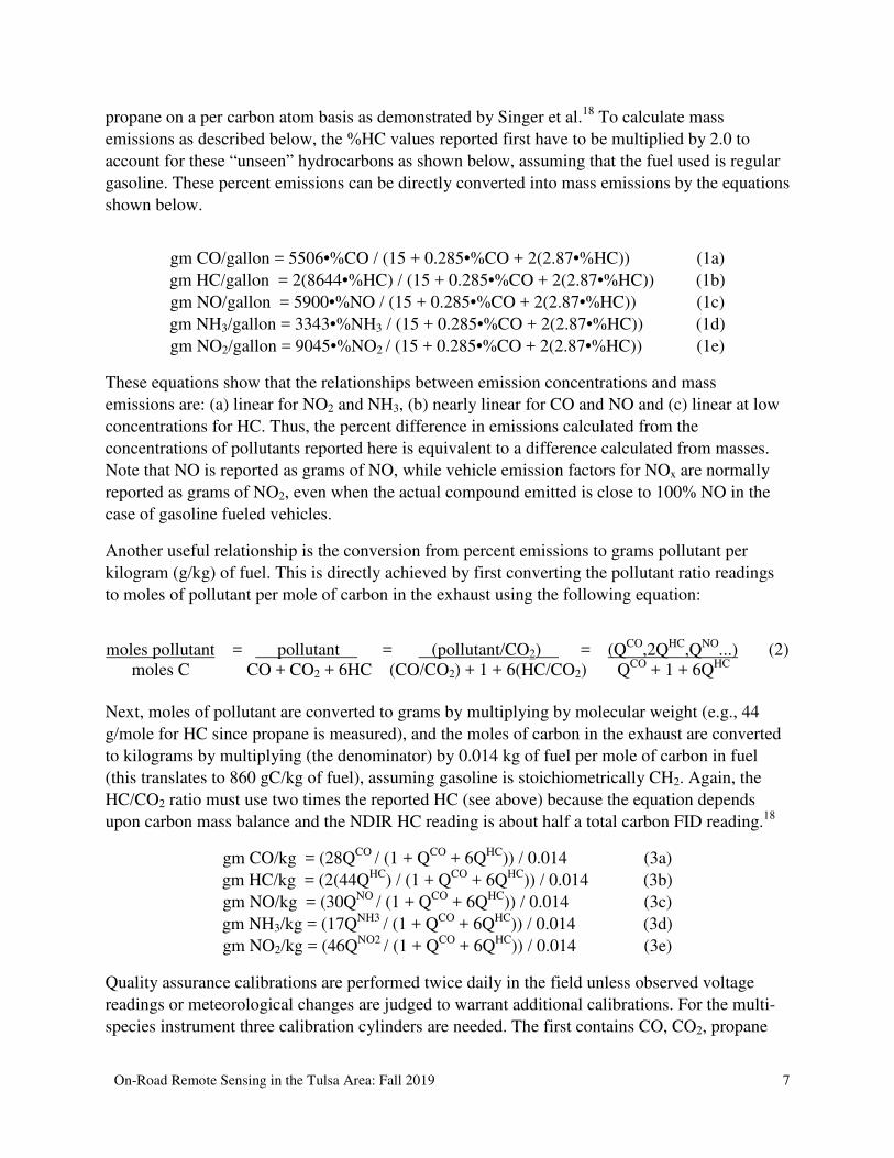
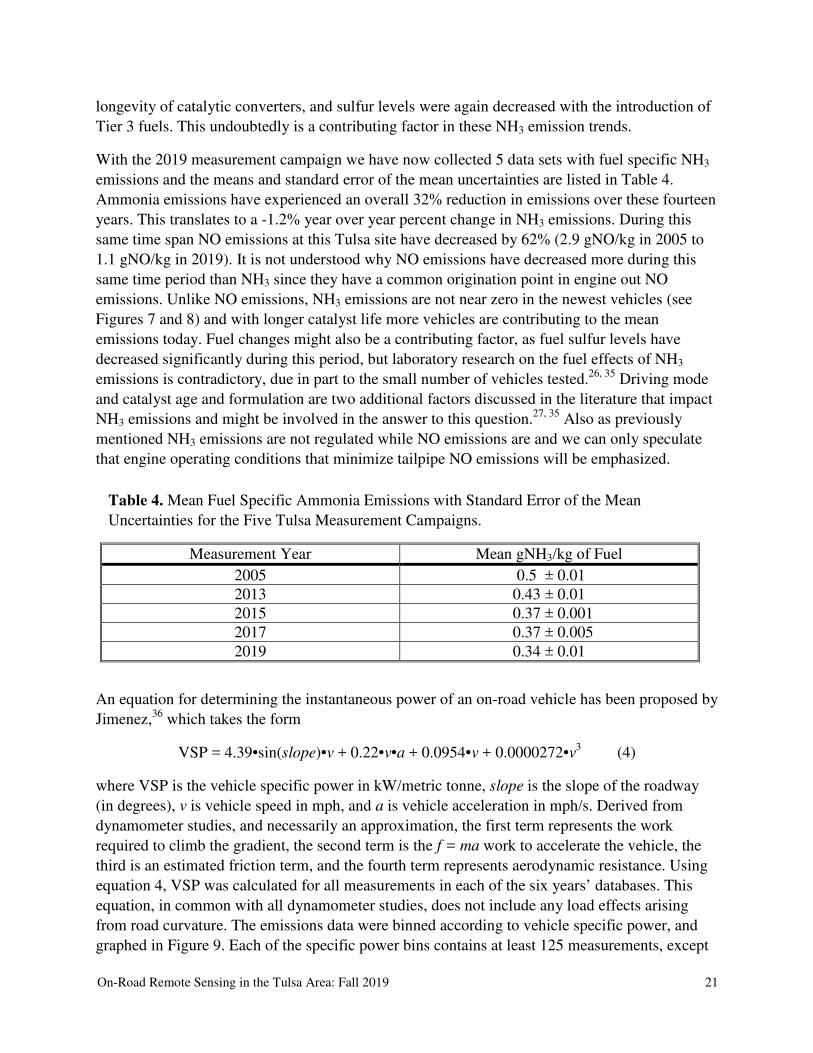
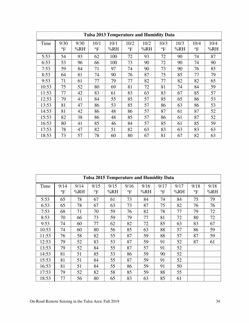