craypat and cray apprentice tri-lab tools workshop … · craypat and cray apprentice tri-lab tools...

CrayPat and Cray ApprenticeTri-Lab Tools WorkshopMarch 24, 2010 @ SNLMarch 25, 2010 @LANL

Mahesh Rajan

Sandia National Lab

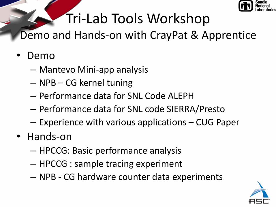
Tri-Lab Tools WorkshopDemo and Hands-on with CrayPat & Apprentice

• Demo– Mantevo Mini-app analysis

– NPB – CG kernel tuning

– Performance data for SNL Code ALEPH

– Performance data for SNL code SIERRA/Presto

– Experience with various applications – CUG Paper

• Hands-on– HPCCG: Basic performance analysis

– HPCCG : sample tracing experiment

– NPB - CG hardware counter data experiments

Mantevo Mini-App: HPCCG • Mike Heroux’s Conjugate Gradient mini-app• Most of the time dominated by sparse Matrix Vector multiplication• Parallel overhead small fraction of run time • On HPC systems with multi-core/multi-socket nodes it nicely brings out the performance impact of the memory bandwidth

0

10

20

30

40

50

60

70

1 10 100 1000 10000

Wal

l Tim

e, s

ecs

Number of MPI Tasks

Mini-Application HPCCG; Weak Scaling;Wall Times, secs

Red Storm Quad

TLCC

RedSky- NUMA

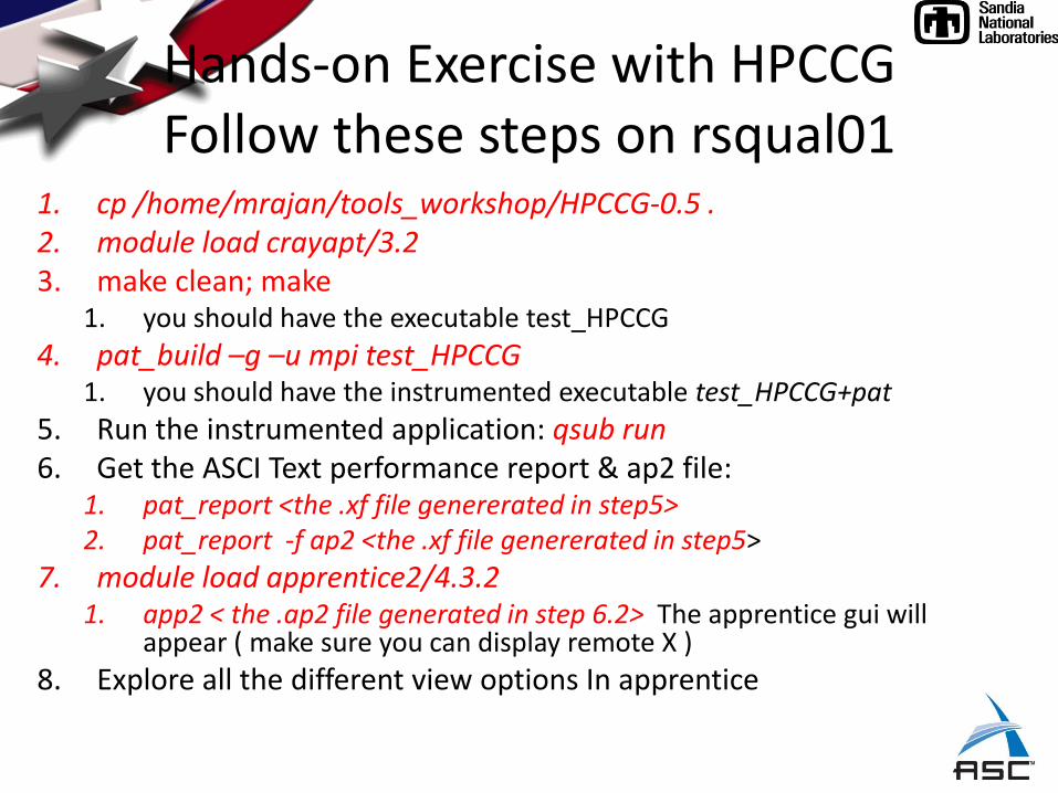
Hands-on Exercise with HPCCGFollow these steps on rsqual01

1. cp /home/mrajan/tools_workshop/HPCCG-0.5 .2. module load crayapt/3.23. make clean; make

1. you should have the executable test_HPCCG

4. pat_build –g –u mpi test_HPCCG1. you should have the instrumented executable test_HPCCG+pat

5. Run the instrumented application: qsub run6. Get the ASCI Text performance report & ap2 file:

1. pat_report <the .xf file genererated in step5>2. pat_report -f ap2 <the .xf file genererated in step5>

7. module load apprentice2/4.3.21. app2 < the .ap2 file generated in step 6.2> The apprentice gui will

appear ( make sure you can display remote X )

8. Explore all the different view options In apprentice

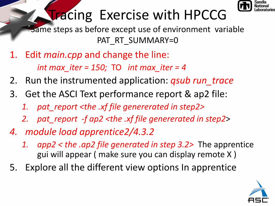
Tracing Exercise with HPCCGSame steps as before except use of environment variable

PAT_RT_SUMMARY=0

1. Edit main.cpp and change the line:int max_iter = 150; TO int max_iter = 4

2. Run the instrumented application: qsub run_trace

3. Get the ASCI Text performance report & ap2 file: 1. pat_report <the .xf file genererated in step2>

2. pat_report -f ap2 <the .xf file genererated in step2>

4. module load apprentice2/4.3.21. app2 < the .ap2 file generated in step 3.2> The apprentice

gui will appear ( make sure you can display remote X )

5. Explore all the different view options In apprentice

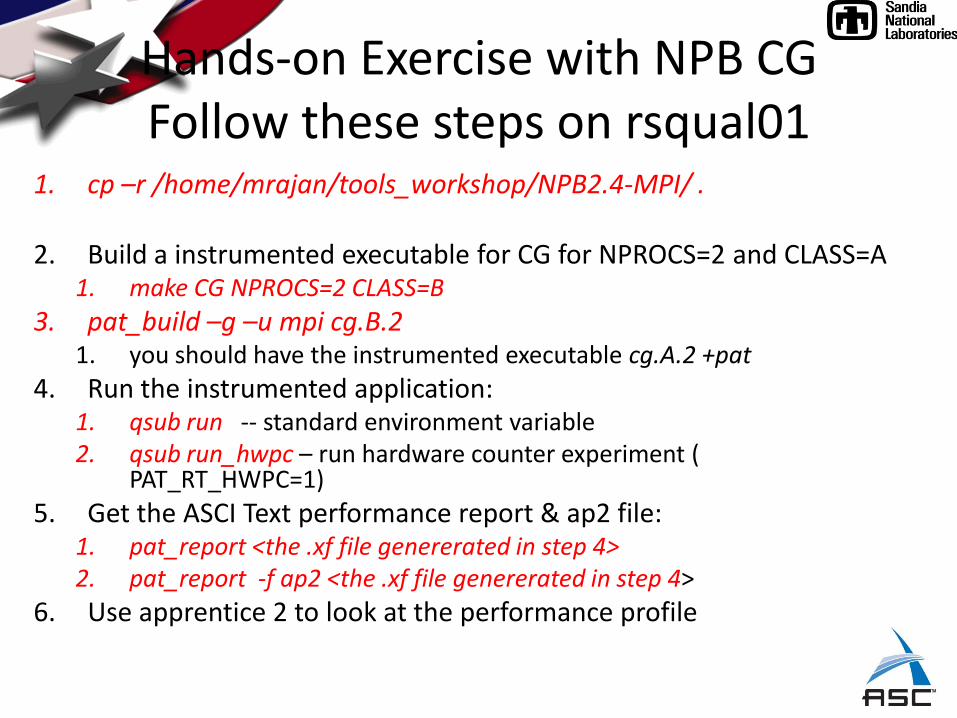
Hands-on Exercise with NPB CGFollow these steps on rsqual01

1. cp –r /home/mrajan/tools_workshop/NPB2.4-MPI/ .

2. Build a instrumented executable for CG for NPROCS=2 and CLASS=A1. make CG NPROCS=2 CLASS=B

3. pat_build –g –u mpi cg.B.21. you should have the instrumented executable cg.A.2 +pat

4. Run the instrumented application: 1. qsub run -- standard environment variable2. qsub run_hwpc – run hardware counter experiment (

PAT_RT_HWPC=1)

5. Get the ASCI Text performance report & ap2 file: 1. pat_report <the .xf file genererated in step 4>2. pat_report -f ap2 <the .xf file genererated in step 4>

6. Use apprentice 2 to look at the performance profile

Hands-on Exercise with NPB CGPerformance Tuning with Loop unrolling and prefetching

1. cp cg.f cg.f.orig; cp cg_tuned.f cg.f

2. Build a instrumented executable for CG for NPROCS=2 and CLASS=A1. make CG NPROCS=2 CLASS=A

3. pat_build –g –u mpi cg.A.21. you should have the instrumented executable cg.A.2 +pat

4. Run the instrumented application: 1. qsub run -- standard environment variable2. qsub run_hwpc – run hardware counter experiment ( PAT_RT_HWPC=1)

5. Get the ASCI Text performance report & ap2 file: 1. pat_report <the .xf file genererated in step 4>2. pat_report -f ap2 <the .xf file genererated in step 4>

6. Use apprentice 2 to look at the performance profile7. Observe that it is not straight forward to relate performance improvement

to PAPI_L1_DCM or PAPI_L2_DCM

8M. Rajan

Experiences with the use of CrayPat in Performance Analysis

Mahesh RajanSandia National Laboratories, Albuquerque, NM

Cray User GroupSeattle, WA; May 7-10, 2007

Sandia is a multi-program laboratory operated by Sandia Corporation, a Lockheed Martin Company,for the United States Department of Energy’s National Nuclear Security Administration

under contract DE-AC04-94AL85000.

3/23/2010 9M. Rajan

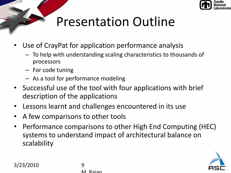
Presentation Outline

• Use of CrayPat for application performance analysis– To help with understanding scaling characteristics to thousands of

processors

– For code tuning

– As a tool for performance modeling

• Successful use of the tool with four applications with brief description of the applications

• Lessons learnt and challenges encountered in its use

• A few comparisons to other tools

• Performance comparisons to other High End Computing (HEC) systems to understand impact of architectural balance on scalability

3/23/2010 10M. Rajan

Applications Investigated

• ICARUS DSMC – Low density MC flow code

• POP – Ocean Modeling

• LAMMPS – Molecular Dynamics

• ITS – MC Particle Radiation Transport

• Few simple math kernels

• HPCCG – Sparse Solver/Conjugate gradient kernel

3/23/2010 11M. Rajan

DSMC/ICARUS for MEMSOscillating microbeam in low density fluid

Moving Micro devices; Rotating Gear, Comb Drives, pop-up mirror,

Oscillating Microbeams

Oscillating Microbeam: Transient pressure fields: left, 250 ns; right, 750 ns

Application Characteristics;

Monte Carlo (DSMC) method is the only proven method for simulating non-continuum gas flows because continuum methods break down where particles move in ballistic trajectories with mean free path larger than cell dimensions, often because the device is small ( micro-or nano-technology) or the fluid is very low pressure as in plasma or upper atmosphere

Particles (simulators) are allowed to move, collide and exchange energy

Computation domain decomposed into cells and cells assigned to processors (scattered or geometric)

Particle information is exchanged with the ‘target’ processor after each

computation step

Acknowledgment: John Torczynski, Michail Gallis, Dan Rader, Steve Plimpton

3/23/2010 12M. Rajan

DSMC PerformanceICARUS DSMC; Execution Time

Weak Scaling with 8125 simulators/cell/PE

0

0.005

0.01

0.015

0.02

0.025

0.03

0 256 512 768 1024 1280 1536 1792 2048

Number of Processors

Exe

cutio

n Ti

me,

hrs Thunderbird

Red Storm

The major computational stages at each time step are:create particlesmove particlescommunicate particles that have moved to cell owned by another processorif (mod(step,stat_out))print stat compute electron / particle chemistrycompute Monte Carlo collisionssolve EM fieldoutput cell, surf data at requested frequency

Problem Parameters:8125 simulators per cell/PEdomain meshed with 52,000, 0.05-mm square cells time step is 0.1 ns and benchmark measures run time for1000 time steps

Property Nominal Value

Gas Nitrogen

Ambient pressure 84 kPa

Temperature 295 K

Beam width 20 m

Beam thickness 2 m

Gap height 2 m

Oscillation frequency 1 MHz

Velocity amplitude 1 m/s

Microbeam properties

3/23/2010 13M. Rajan

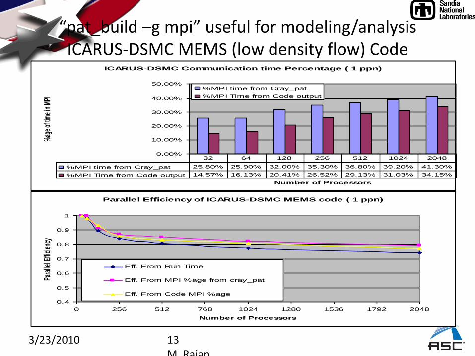
“pat_build –g mpi” useful for modeling/analysis ICARUS-DSMC MEMS (low density flow) Code

ICARUS-DSMC Communication time Percentage ( 1 ppn)

0.00%

10.00%

20.00%

30.00%

40.00%

50.00%


%ag

e of t

ime i

n MP

I

%MPI time from Cray_pat

%MPI Time from Code output

%MPI time from Cray_pat 25.80% 25.90% 32.00% 35.30% 36.80% 39.20% 41.30%

%MPI Time from Code output 14.57% 16.13% 20.41% 26.52% 29.13% 31.03% 34.15%

32 64 128 256 512 1024 2048

Parallel Efficiency of ICARUS-DSMC MEMS code ( 1 ppn)

0.4

0.5

0.6

0.7

0.8

0.9

1

0 256 512 768 1024 1280 1536 1792 2048


Para

llel E

fficie

ncy

Eff. From Run Time

Eff. From MPI %age from cray_pat

Eff. From Code MPI %age

3/23/2010 14M. Rajan

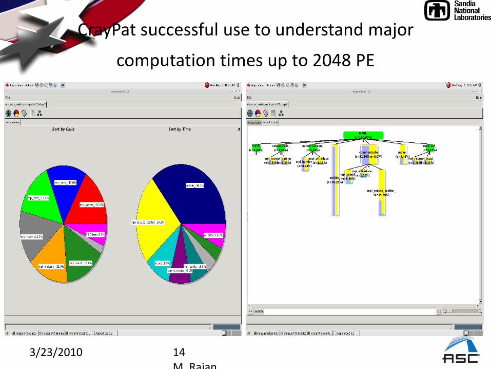
CrayPat successful use to understand major

computation times up to 2048 PE

3/23/2010 15M. Rajan

MPI_Reduce_scatter 41% at 2048 PEs

But load imbalance in ‘move’ impacts parallel Efficiency

3/23/2010 16M. Rajan

CrayPat Trace on 32PEs reveals communication patterns and overheads

3/23/2010 17M. Rajan

Vampir used on Thunderbird for constructing a performance model

3/23/2010 18M. Rajan

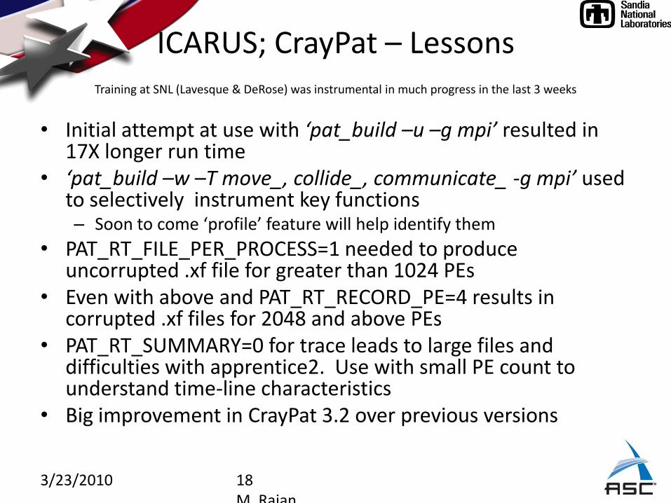
ICARUS; CrayPat – LessonsTraining at SNL (Lavesque & DeRose) was instrumental in much progress in the last 3 weeks

• Initial attempt at use with ‘pat_build –u –g mpi’ resulted in 17X longer run time

• ‘pat_build –w –T move_, collide_, communicate_ -g mpi’ used to selectively instrument key functions– Soon to come ‘profile’ feature will help identify them

• PAT_RT_FILE_PER_PROCESS=1 needed to produce uncorrupted .xf file for greater than 1024 PEs

• Even with above and PAT_RT_RECORD_PE=4 results in corrupted .xf files for 2048 and above PEs

• PAT_RT_SUMMARY=0 for trace leads to large files and difficulties with apprentice2. Use with small PE count to understand time-line characteristics

• Big improvement in CrayPat 3.2 over previous versions

3/23/2010 19M. Rajan

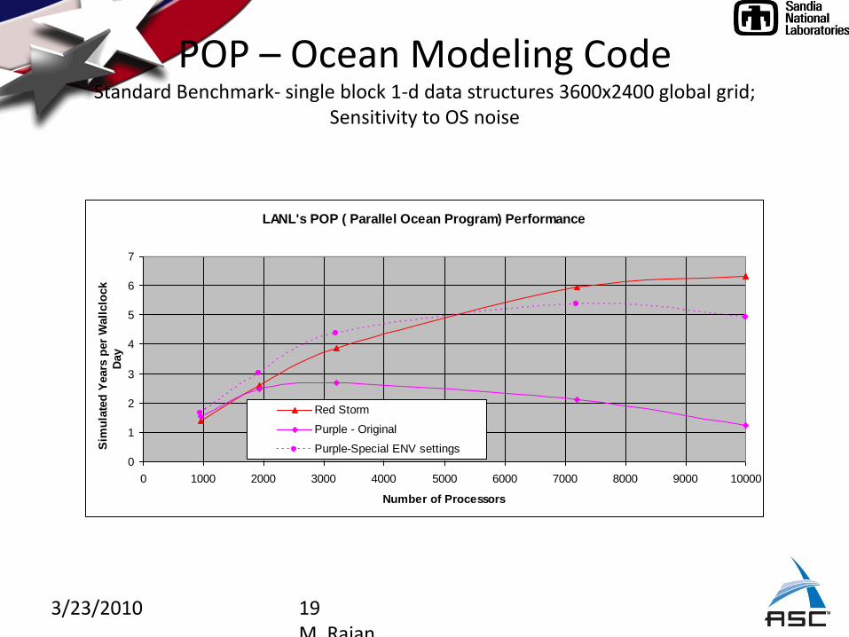
POP – Ocean Modeling CodeStandard Benchmark- single block 1-d data structures 3600x2400 global grid;

Sensitivity to OS noise

LANL's POP ( Parallel Ocean Program) Performance

0

1

2

3

4

5

6

7

0 1000 2000 3000 4000 5000 6000 7000 8000 9000 10000


Sim

ula

ted

Years

per

Wall

clo

ck

Day

Red Storm

Purple - Original

Purple-Special ENV settings

3/23/2010 20M. Rajan

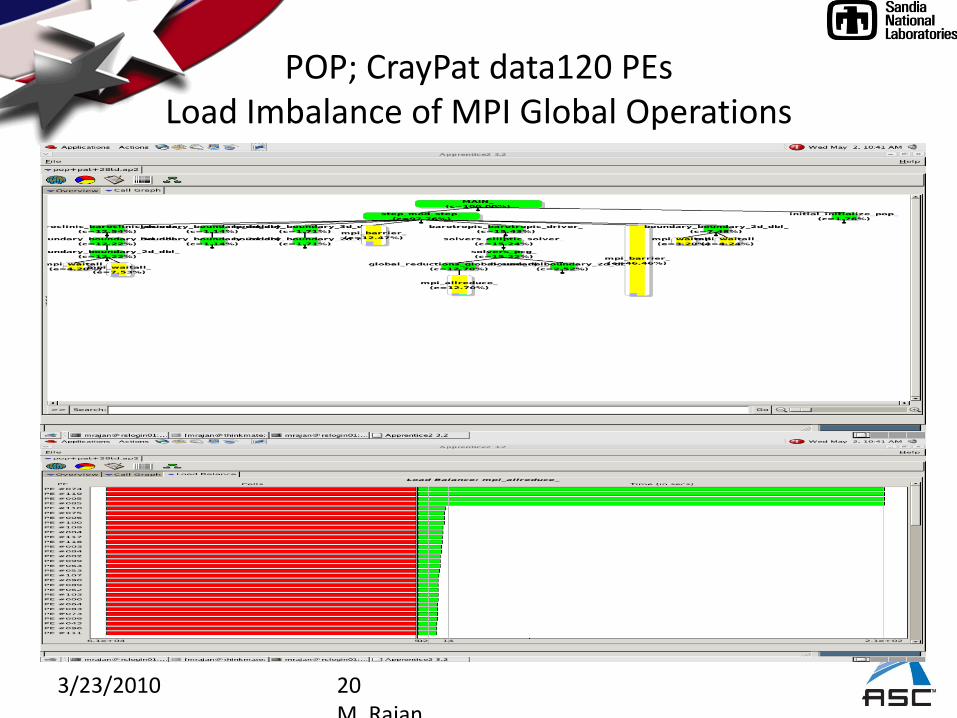
POP; CrayPat data120 PEsLoad Imbalance of MPI Global Operations

3/23/2010 21M. Rajan

POP; CrayPat 120 PEs

Table 1: Profile by Function Group and Function

Time % | Time | Imb. Time | Imb. | Calls |Experiment=1| | | Time % | |Group| | | | | Function| | | | | PE='HIDE'

100.0% | 1740.568341 | -- | -- | 136827465 |Total|---------------------------------------------------------------------| 93.7% | 1630.995416 | -- | -- | 240 |USER||--------------------------------------------------------------------|| 100.0% | 1630.995381 | 86.958475 | 5.1% | 120 |main||====================================================================| 6.3% | 109.572875 | -- | -- | 136779225 |MPI||--------------------------------------------------------------------|| 59.6% | 65.329857 | 1453.807844 | 96.5% | 180000 |mpi_barrier_|| 22.3% | 24.383676 | 51.996170 | 68.6% | 45080035 |mpi_waitall_|| 13.9% | 15.284169 | 203.248604 | 93.8% | 7515600 |mpi_allreduce_|| 1.6% | 1.763033 | 0.312892 | 15.2% | 41970960 |mpi_isend_|| 1.6% | 1.712108 | 0.434041 | 20.4% | 58800 |mpi_bcast_|| 1.0% | 1.099047 | 0.654813 | 37.6% | 41971075 |mpi_irecv_|=====================================================================

3/23/2010 22M. Rajan

POP; CrayPat data; 120 PEs

Table 3: MPI Sent Message Stats by Caller

Sent Msg | Sent Msg | 256B<= | 4KB<= | 64KB<= |Experiment=1Total Bytes | Count | MsgSz | MsgSz | MsgSz |Function

| | <4KB | <64KB | <1MB | Caller| | Count | Count | Count | PE[mmm]

247605586368 | 41971075 | 21762720 | 20208240 | 115 |Total||||=================================================================3|| 81892274688 | 13883184 | 7198688 | 6684496 | -- |solvers_pcg_4|| | | | | | solvers_elliptic_solver_5|| | | | | | barotropic_barotropic_driver_6|| | | | | | step_mod_step_7|| | | | | | MAIN_8|| | | | | | main|||||||||------------------------------------------------------------9|||||||| 771288000 | 128548 | 64274 | 64274 | -- |pe.339|||||||| 771288000 | 128548 | 64274 | 64274 | -- |pe.1009|||||||| 0 | -- | -- | -- | -- |pe.5|||||||||============================================================

3/23/2010 23M. Rajan

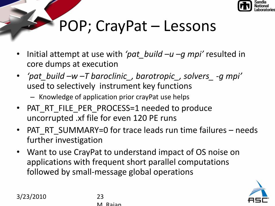
POP; CrayPat – Lessons

• Initial attempt at use with ‘pat_build –u –g mpi’ resulted in core dumps at execution

• ‘pat_build –w –T baroclinic_, barotropic_, solvers_ -g mpi’used to selectively instrument key functions– Knowledge of application prior crayPat use helps

• PAT_RT_FILE_PER_PROCESS=1 needed to produce uncorrupted .xf file for even 120 PE runs

• PAT_RT_SUMMARY=0 for trace leads run time failures – needs further investigation

• Want to use CrayPat to understand impact of OS noise on applications with frequent short parallel computations followed by small-message global operations

3/23/2010 24M. Rajan

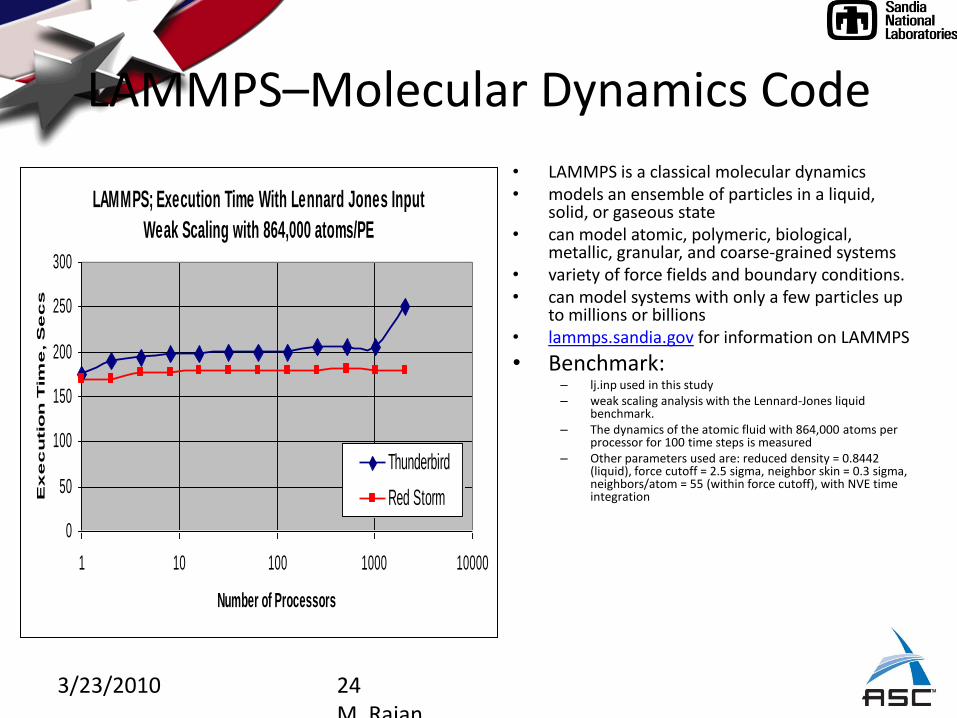
LAMMPS–Molecular Dynamics Code

• LAMMPS is a classical molecular dynamics• models an ensemble of particles in a liquid,

solid, or gaseous state• can model atomic, polymeric, biological,

metallic, granular, and coarse-grained systems• variety of force fields and boundary conditions. • can model systems with only a few particles up

to millions or billions• lammps.sandia.gov for information on LAMMPS

• Benchmark: – lj.inp used in this study– weak scaling analysis with the Lennard-Jones liquid

benchmark. – The dynamics of the atomic fluid with 864,000 atoms per

processor for 100 time steps is measured– Other parameters used are: reduced density = 0.8442

(liquid), force cutoff = 2.5 sigma, neighbor skin = 0.3 sigma, neighbors/atom = 55 (within force cutoff), with NVE time integration

LAMMPS; Execution Time With Lennard Jones Input

Weak Scaling with 864,000 atoms/PE

0

50

100

150

200

250

300

1 10 100 1000 10000


Ex

ec

utio

n T

ime

, S

ec

s

Thunderbird

Red Storm

http://lammps.sandia.gov/doc/Section_perf.html

3/23/2010 25M. Rajan

Good scaling because of good load balance and flat MPI overhead

Num. PEs %MPI time

(CrayPat)

32 1.5

64 2.1

128 1.5

256 2.1

512 1.8

1024 2

2048 2.4

3/23/2010 26M. Rajan

“pat_build –u –g mpi” successful with close to 1500 functions

3/23/2010 27M. Rajan

LAMMPS – CrayPat Analysis2X performance improvement with small pages

3/23/2010 28M. Rajan

LAMMPS – CrayPat AnalysisTable 1: Profile by Function Group and Function

Time % | Time |Imb. Time | Imb. | Calls |Group| | | Time % | | Function| | | | | PE='HIDE'

100.0% | 194.741639 | -- | -- | 651228062 |Total|----------------------------------------------------------------| 97.9% | 190.744605 | -- | -- | 651073918 |USER||---------------------------------------------------------------|| 77.6% | 148.112593 | 3.001152 | 2.1% | 3232 |PairLJCut:compute(int, int)|| 8.7% | 16.511221 | 0.157160 | 1.0% | 192 |Neighbor:pair_bin_newton()||===============================================================| 2.1% | 3.996901 | -- | -- | 141344 |MPI||---------------------------------------------------------------|| 75.3% | 3.009888 | 2.180590 | 43.4% | 39744 |MPI_Send|| 18.1% | 0.725386 | 2.562926 | 80.5% | 39744 |MPI_Wait|| 5.1% | 0.202229 | 0.062096 | 24.3% | 1216 |MPI_Allreduce|| 0.6% | 0.022056 | 0.000839 | 3.8% | 1792 |MPI_Bcast

Table 3: MPI Sent Message Stats by Caller

Sent Msg | Sent | MsgSz | 4KB<= | 64KB<= | 1MB<= |FunctionTotal Bytes | Msg | <16B | MsgSz | MsgSz | MsgSz | Caller

| Count | Count | <64KB | <1MB | <16MB | PE[mmm]| | | Count | Count | Count |

25619726416 | 41856 | 2272 | 2 | 38462 | 1120 |Total|---------------------------------------------------------------| 25619717968 | 39744 | 160 | 2 | 38462 | 1120 |MPI_Send||--------------------------------------------------------------|| 12379279464 | 19392 | -- | -- | 19392 | -- |Comm:reverse_communicate()3| | | | | | | Comm:__wrap_reverse_communicate()||||------------------------------------------------------------4||| 12256252776 | 19200 | -- | -- | 19200 | -- |Verlet:iterate(int)

Small fraction of time in MPI

MPI_send msg sizes are fairly large

3/23/2010 29M. Rajan

ITS-Particle Radiation Transport Problem Investigated

• Satellite combinatorial geometry model; 600 CG bodies

• Calculations performed for this work were adjoint point estimation of KERMA (Kinetic Energy Released per unit Mass

• Asses energy deposition at a point inside of an electronics box in the satellite

• Figure illustrates the dosage computations where the pixels are angular bins of the source directions and the levels are dose values at the same point on the object.

HIGH DOSE

LOW DOSE

infinite-extent

planar sources

3/23/2010 30M. Rajan

Scaling Study and Model• Geometry replicated on all the processors

• Master/Worker computations

– Statistical tally data collected by Master after each batch of computations

• 3.2 million histories per processor, weak scaling analysis

tallysetupioncommunicat TTT

PTNT histphcompute /

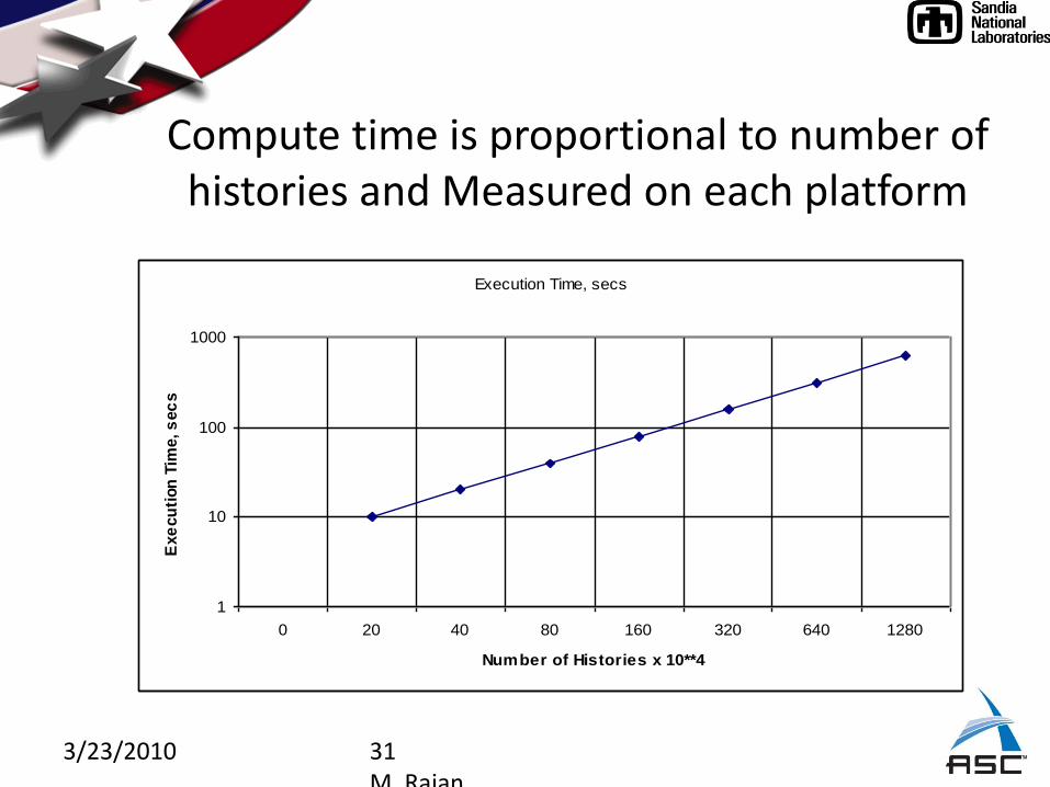
3/23/2010 31M. Rajan

Compute time is proportional to number of histories and Measured on each platform

Execution Time, secs

1

10

100

1000

0 20 40 80 160 320 640 1280

Number of Histories x 10**4

Exe

cu

tion

Tim

e, s

ec

s

3/23/2010 32M. Rajan

VAMPIR trace permitted construction of communication model

Us

er

co

de

User codeMPI_

wait_

all

MPI_

Irecv

Us

er

co

de

MPI_recv Us

er

co

de

Us

er

co

de

MPIIs

end

MPI_

Isend

MPI_

wait_

all

Us

er

co

de

Us

er

co

de

MPI_

Isend

48

byte

s

48

byte

s16.6M

bytes

48000

bytes368

byte

s

432

byte

s

3/23/2010 33M. Rajan

Communication Model

• Master-Worker; Many to one; tally data sent to master

• Tcomm.= {2 * T48 + T48000 + T432 + T16M + T368 } * num_batches * (p-1)

• Input: Latency, Bandwidth(Pt-to-Pt), num_procs(p), num_batches

• Dominant Message size is a function of (maximum Azimuthal, Polar angle, energy bins for escape photon, maximum surface source distributions, num materials, num fluorescence lines)

3/23/2010 34M. Rajan

Model Evaluated on ASC Red, Cplant, Vplant and ICC cluster

ITS Parallel Efficiency, Model vs. Measured

VPLANT

0.5

0.6

0.7

0.8

0.9

1

1 2 4 8 16 32 64 128

256

512


Pa

rall

el

Eff

icie

nc

y

Model, Parallel

Efficiency

Measured, Parallel

Efficiency

Efficiency

Rabenseifners

algorithm


JANUS

0.80.820.840.860.88

0.90.920.940.960.98

1

1 2 4 8

16

32

64

12

8

25

6

51

2

10

24


Pa

rall

el

Eff

icie

nc

y

Model, Parallel

Efficiency

Measured, Parallel

Efficiency


ICC-LIBERTY

0.60.640.680.720.76

0.80.840.880.920.96

1

1 2 4 8 16 32 64 128 256


Pa

rall

el

Eff

icie

nc

y

Model, Parallel

Efficiency

Measured, Parallel

Efficiency


CPLANT

0.3

0.4

0.5

0.6

0.7

0.8

0.9

1

1.1

1 2 4 8

16

32

64

12

8

25

6

51

2

10

24


Pa

rall

el

Eff

icie

nc

y

Model, Parallel

Efficiency

Measured, Parallel

Efficiency

3/23/2010 35M. Rajan

ITS on Red Storm, Parallel Efficiency

Measured and Modeled

ITS Redstorm Parallel Efficiency

0.3

0.4

0.5

0.6

0.7

0.8

0.9

1

1.1

1 10 100 1000 10000

Number of Processes

Para

lle

l E

ffic

ien

cy

Old Code Measured Apr. 05

Old Code Perf. Model

New Code Measured-Global Reduce

Rabenseifner's Algorithm Model

3/23/2010 36M. Rajan

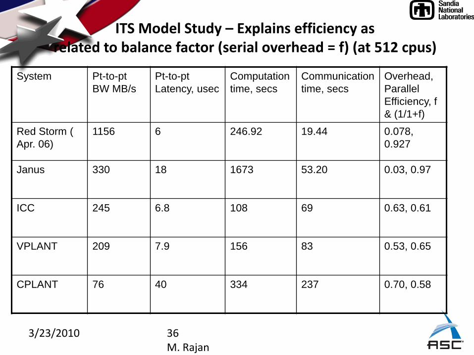
ITS Model Study – Explains efficiency asrelated to balance factor (serial overhead = f) (at 512 cpus)

System Pt-to-pt

BW MB/s

Pt-to-pt

Latency, usec

Computation

time, secs

Communication

time, secs

Overhead,

Parallel

Efficiency, f

& (1/1+f)

Red Storm (

Apr. 06)

1156 6 246.92 19.44 0.078,

0.927

Janus 330 18 1673 53.20 0.03, 0.97

ICC 245 6.8 108 69 0.63, 0.61

VPLANT 209 7.9 156 83 0.53, 0.65

CPLANT 76 40 334 237 0.70, 0.58

3/23/2010 37M. Rajan

ITS – Monte Carlo Particle transportfunction ‘dista_’ used to track particle in the zone/object geometry; has nested condition blocks;

‘ran_’ psuedo-random number generator;

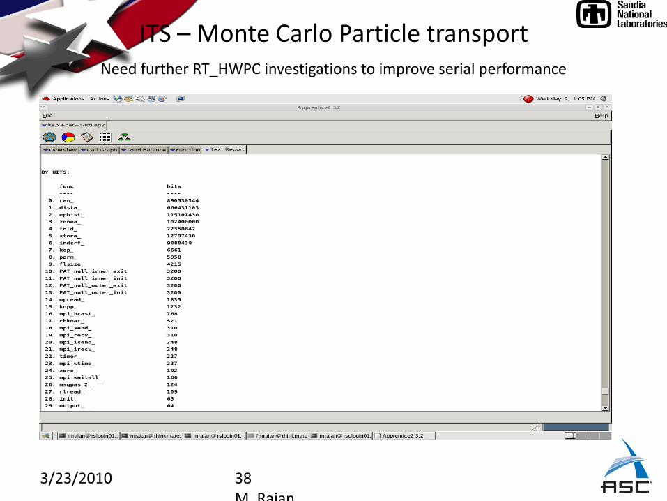
3/23/2010 38M. Rajan

ITS – Monte Carlo Particle transportNeed further RT_HWPC investigations to improve serial performance

3/23/2010 39M. Rajan

Single CPU Performance Tuning and PAPI analysis

Processor Opteron Power3 Itanium

Exec. time, secs 1.69 6.51 3.91

Comparison of single processor execution time:Opteron 2GHz: L1=64KB, L2=1MB Power3, 375 MHz, L1=64KB (Data); 32KB (Ins), L2=8MB Itanium-2, 1.4GHz, L1=32KB, L2=256KB, L3=3MB

Compute time does not significantly reduce with cache size

GPROF shows On Itanium dista_ children:

gg(56%), loczon(10%), and locbod(7%)

GPROF shows on Opteron dista_ children :

gg(70%), loczon(9%), and locbod(6%).

Subroutine gg mainly consists of branches for different geometries such a polyhedron, sphere, cone, cylinder, etc. Further within the computations for each geometrical body there are branches to compute intersection of particle trajectory lines with geometry component surfaces and for different directions of travel.

3/23/2010 40M. Rajan

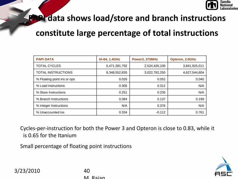
PAPI data shows load/store and branch instructions

constitute large percentage of total instructions

PAPI DATA IA-64, 1.4GHz Power3, 375MHz Opteron, 2.0GHz

TOTAL CYCLES 5,471,391,792 2,524,426,100 3,841,925,011

TOTAL INSTRUCTIONS 8,348,552,835 3,022,782,250 4,627,544,804

% Floating point ins or ops 0.026 0.052 0.040

% Load instructions 0.305 0.312 N/A

% Store Instructions 0.251 0.235 N/A

% Branch Instructions 0.084 0.137 0.199

% Integer Instructions N/A 0.376 N/A

% Unaccounted ins 0.334 -0.112 0.761

Cycles-per-instruction for both the Power 3 and Opteron is close to 0.83, while it is 0.65 for the Itanium

Small percentage of floating point instructions

3/23/2010 41M. Rajan

Single Processor Performance improvement

• No easy choice of code modifications to improve performance

• Need to improve cache temporal locality, but the structure of the code containing major loop over the histories, suggests that dista_ computations would invoke bringing different geometry data into cache

• Compiler optimization on Power3 using inter-procedural analysis (ipa) yielded 47% improvement.

• Similar ipa options on Opteron and IA-64 yielded negligible performance improvement

3/23/2010 42M. Rajan

ITS; CrayPat – Lessons

• CrayPat/HWPC much easier to use than prior use approaches with PAPI-API– Code dominated by non-floating point ops; AMD needs to

provide load, store, integer counters

• Need further experimentation with trace• One 32 PE trace file / .ap2 took a very long time to

load into apprentice• Vampir like message statistics plot will be useful; also

ability to click and look at message characteristics in zoomed trace plots helpful for performance modeling

3/23/2010 43M. Rajan

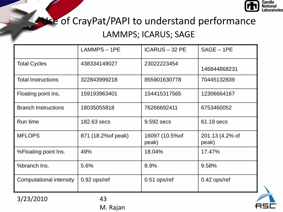
Use of CrayPat/PAPI to understand performanceLAMMPS; ICARUS; SAGE

LAMMPS – 1PE ICARUS – 32 PE SAGE – 1PE

Total Cycles 438334149027 23022223454146844868231

Total Instructions 322843999218 855901630778 70445132839

Floating point ins. 159193963401 154415317565 12306664167

Branch Instructions 18035055818 76266692411 6753460052

Run time 182.63 secs 9.592 secs 61.18 secs

MFLOPS 871 (18.2%of peak) 16097 (10.5%of

peak)

201.13 (4.2% of

peak)

%Floating point Ins. 49% 18.04% 17.47%

%branch Ins. 5.6% 8.9% 9.58%

Computational intensity 0.92 ops/ref 0.51 ops/ref 0.42 ops/ref

3/23/2010 44M. Rajan

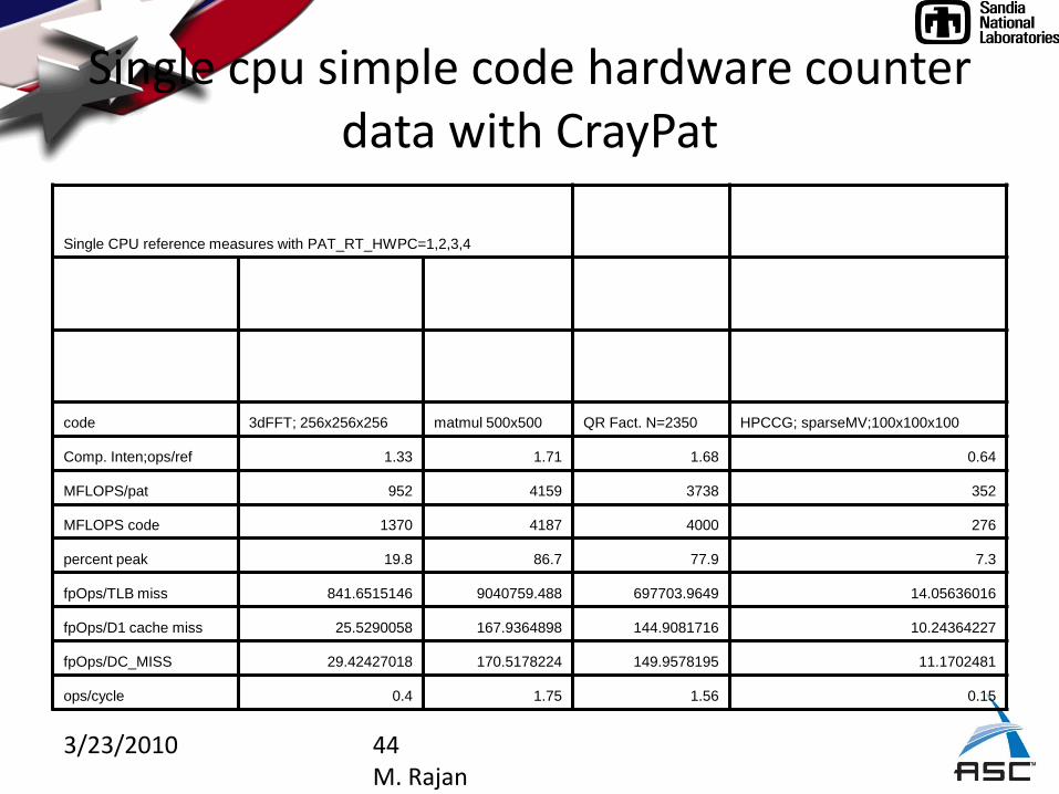
Single cpu simple code hardware counter data with CrayPat

Single CPU reference measures with PAT_RT_HWPC=1,2,3,4

code 3dFFT; 256x256x256 matmul 500x500 QR Fact. N=2350 HPCCG; sparseMV;100x100x100

Comp. Inten;ops/ref 1.33 1.71 1.68 0.64

MFLOPS/pat 952 4159 3738 352

MFLOPS code 1370 4187 4000 276

percent peak 19.8 86.7 77.9 7.3

fpOps/TLB miss 841.6515146 9040759.488 697703.9649 14.05636016

fpOps/D1 cache miss 25.5290058 167.9364898 144.9081716 10.24364227

fpOps/DC_MISS 29.42427018 170.5178224 149.9578195 11.1702481

ops/cycle 0.4 1.75 1.56 0.15

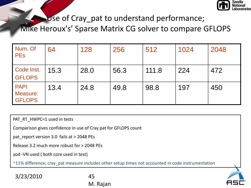
3/23/2010 45M. Rajan

Use of Cray_pat to understand performance; Mike Heroux's’ Sparse Matrix CG solver to compare GFLOPS

Num. Of

PEs64 128 256 512 1024 2048

Code Inst.

GFLOPS

15.3 28.0 56.3 111.8 224 472

PAPI

Measure:

GFLOPS

13.4 24.8 49.8 98.8 197 450

PAT_RT_HWPC=1 used in tests

Comparison gives confidence in use of Cray pat for GFLOPS count

pat_report version 3.0 fails at > 2048 PEs

Release 3.2 much more robust for > 2048 PEs

yod -VN used ( both core used in test)

~11% difference; cray_pat measure includes other setup times not accounted in code instrumentation

3/23/2010 46M. Rajan

Conclusions • Ease of use is very nice!• CrayPat and Apprentice are both feature rich! • Helping with developing performance model for DSMC-

ICARUS• Helped to validate ITS performance model• ‘profile’ feature in future release will help improve

productivity• Limited experience with trace, but nice to see features like in

VAMPIR – robustness needs improvement?• Large PE experiments showed lustre/file corruption problems• Early experiments have been successful with a number of

applications, but anticipate the tool will be stressed with SNL’s SIERRA codes

3/23/2010 47M. Rajan

Planned use of CrayPat

• Try to quantify the gap between peak performance and sustained; It is widening – Multi-core archichitecture racing ahead of concurrency– Memory bottlenecks

• Performance modeling• Tool for capability computing, to identify scaling

limitations and remedies• Next generation architecture research; Impact of

architectural balance

craypat and cray apprentice tri-lab tools workshop … · craypat and cray apprentice tri-lab tools...

Documents