crava user manual

Note no SAND/05/2012Authors Pål Dahle

Bjørn FjellvollFrode GeorgsenRagnar Hauge

Odd KolbjørnsenAnne Randi SyversveenMarit Ulvmoen

Date March 2, 2012

CRAVA User Manualversion 1.2

Pål DahleBjørn Fjellvoll Frode GeorgsenRagnar HaugeOdd KolbjørnsenAnne Randi SyversveenMarit Ulvmoen

The authorsPål Dahle is a Senior Research Scientist at NR,Bjørn Fjellvoll is a Research Scientist at NR,Frode Georgsen is a Senior Research Scientist at NR.Ragnar Hauge is an Assistant Research Director at NR,Odd Kolbjørnsen is a Chief Research Scientist at NR,Anne Randi Syversveen is a Senior Research Scientist at NR andMarit Ulvmoen is a Research Scientist at NR.

Norwegian Computing CenterNorsk Regnesentral (Norwegian Computing Center, NR) is a private, independent, non-profitfoundation established in 1952. NR carries out contract research and development projects ininformation and communication technology and applied statistical-mathematical modelling. Theclients include a broad range of industrial, commercial and public service organisations in thenational as well as the international market. Our scientific and technical capabilities are furtherdeveloped in co-operation with The Research Council of Norway and key customers. The resultsof our projects may take the form of reports, software, prototypes, and short courses. A proof ofthe confidence and appreciation our clients have in us is given by the fact that most of our newcontracts are signed with previous customers.

Title CRAVA User Manual version 1.2

Authors Pål Dahle, Bjørn Fjellvoll , Frode Georgsen, Ragnar Hauge,Odd Kolbjørnsen, Anne Randi Syversveen, Marit Ulvmoen

Date March 2, 2012

Publication number SAND/05/2012

AbstractCRAVA is a simple inversion tool, particularly suited for quick generation of first pass inversionsand facies probabilities for use in geological modeling. This manual describes the theory behind,the main implementation structure, and the actual use of this program.

Keywords CRAVA, seismic, inversion, geostatistical, Bayesian, AVO, FFT

Target group NR, Statoil, Norsar, Roxar

Availability Open

Project -

Project number -

Research field Reservoir characterisation

Number of pages 93

Copyright © 2012 Norwegian Computing Center

3

Contents

1 Model . . . . . . . . . . . . . . . . . . . . . . . . . . . . . 14

1.1 Introduction . . . . . . . . . . . . . . . . . . . . . . . . . 14

1.2 AVO . . . . . . . . . . . . . . . . . . . . . . . . . . . 14

1.3 Seismic model . . . . . . . . . . . . . . . . . . . . . . . . 15

1.3.1 Convolution with 3D wavelet . . . . . . . . . . . . . . . 16

1.4 Statistical model . . . . . . . . . . . . . . . . . . . . . . . 16

1.4.1 Facies probabilities . . . . . . . . . . . . . . . . . . . 18

2 Implementation . . . . . . . . . . . . . . . . . . . . . . . . . 22

2.1 Estimating optimal well location. . . . . . . . . . . . . . . . . . 22

2.2 Estimating the prior model . . . . . . . . . . . . . . . . . . . 22

2.2.1 Background model . . . . . . . . . . . . . . . . . . . 22

2.2.2 Covariance. . . . . . . . . . . . . . . . . . . . . . 25

2.2.3 Likelihood model. . . . . . . . . . . . . . . . . . . . 25

2.3 Estimating wavelets . . . . . . . . . . . . . . . . . . . . . . 25

2.4 Estimating 3D wavelet . . . . . . . . . . . . . . . . . . . . . 28

2.5 Using FFT for inversion. . . . . . . . . . . . . . . . . . . . . 28

2.6 A note one local wavelet and noise . . . . . . . . . . . . . . . . 28

2.6.1 Local wavelet - dividing out the wavelet . . . . . . . . . . . 28

2.6.2 Local noise. . . . . . . . . . . . . . . . . . . . . . 29

2.7 Memory handling . . . . . . . . . . . . . . . . . . . . . . . 29

2.7.1 Grid allocation with all grids in memory . . . . . . . . . . . 29

3 User guide . . . . . . . . . . . . . . . . . . . . . . . . . . . 31

3.1 Basic inversion. . . . . . . . . . . . . . . . . . . . . . . . 31

3.1.1 Survey information . . . . . . . . . . . . . . . . . . . 31

3.1.1.1 Seismic data . . . . . . . . . . . . . . . . . . . . . . . . . . . . . . . 32

3.1.1.2 Wavelet . . . . . . . . . . . . . . . . . . . . . . . . . . . . . . . . . . 32

3.1.1.3 Signal/noise ratio . . . . . . . . . . . . . . . . . . . . . . . . . . . . 33

3.1.2 Inversion volume. . . . . . . . . . . . . . . . . . . . 33

3.1.2.1 Lateral extent . . . . . . . . . . . . . . . . . . . . . . . . . . . . . . . 33

3.1.2.2 Top and base surfaces . . . . . . . . . . . . . . . . . . . . . . . . . . 34

3.1.2.3 Depth conversion . . . . . . . . . . . . . . . . . . . . . . . . . . . . 35

CRAVA User Manual version 1.2 4

3.1.3 Prior model . . . . . . . . . . . . . . . . . . . . . 36

3.1.3.1 Background model . . . . . . . . . . . . . . . . . . . . . . . . . . . 36

3.1.3.2 Covariances . . . . . . . . . . . . . . . . . . . . . . . . . . . . . . . 37

3.1.4 Well data . . . . . . . . . . . . . . . . . . . . . . 37

3.1.5 I/O settings. . . . . . . . . . . . . . . . . . . . . . 38

3.1.6 Output . . . . . . . . . . . . . . . . . . . . . . . 38

3.1.6.1 Grid output . . . . . . . . . . . . . . . . . . . . . . . . . . . . . . . . 39

3.1.6.2 Well output . . . . . . . . . . . . . . . . . . . . . . . . . . . . . . . . 39

3.1.7 Actions . . . . . . . . . . . . . . . . . . . . . . . 40

3.1.8 Standard grid formats . . . . . . . . . . . . . . . . . . 40

3.2 Advanced inversion options . . . . . . . . . . . . . . . . . . . 41

3.2.1 Non-stationary wavelet and noise . . . . . . . . . . . . . 41

3.2.2 PS-seismic and reflection approximations. . . . . . . . . . . 41

3.2.3 Well quality checks . . . . . . . . . . . . . . . . . . . 42

3.2.4 Generate synthetic seismic from inversion data . . . . . . . . 42

3.3 Estimation . . . . . . . . . . . . . . . . . . . . . . . . . 42

3.3.1 Estimation mode. . . . . . . . . . . . . . . . . . . . 42

3.3.2 Wavelet and noise estimation . . . . . . . . . . . . . . . 43

3.3.3 Background model estimation . . . . . . . . . . . . . . . 43

3.3.4 Prior correlations . . . . . . . . . . . . . . . . . . . 44

3.4 3D wavelet . . . . . . . . . . . . . . . . . . . . . . . . . 44

3.5 Facies prediction . . . . . . . . . . . . . . . . . . . . . . . 44

3.5.1 Prior probabilities . . . . . . . . . . . . . . . . . . . 46

3.5.2 Output parameters . . . . . . . . . . . . . . . . . . . 46

3.6 Forward modelling . . . . . . . . . . . . . . . . . . . . . . 46

4 Model file reference manual . . . . . . . . . . . . . . . . . . . . . 48

4.1 <actions> (necessary) . . . . . . . . . . . . . . . . . . . . . 48

4.1.1 <mode> (necessary) . . . . . . . . . . . . . . . . . . . 48

4.1.2 <inversion-settings> . . . . . . . . . . . . . . . . . 48

4.1.2.1 <prediction> . . . . . . . . . . . . . . . . . . . . . . . . . . . . . . 48

4.1.2.2 <simulation> . . . . . . . . . . . . . . . . . . . . . . . . . . . . . . 48

4.1.2.2.1 <seed> . . . . . . . . . . . . . . . . . . . . . . . . . . . . . 48

4.1.2.2.2 <seed-file> . . . . . . . . . . . . . . . . . . . . . . . . . . 49

4.1.2.2.3 <number-of-simulations> . . . . . . . . . . . . . . . . . 49

4.1.2.3 <kriging-to-wells> . . . . . . . . . . . . . . . . . . . . . . . . . . 49

4.1.2.4 <facies-probabilities> . . . . . . . . . . . . . . . . . . . . . . . 49


4.1.3 <estimation-settings> . . . . . . . . . . . . . . . . . 49

4.1.3.1 <estimate-background> . . . . . . . . . . . . . . . . . . . . . . . . 49

4.1.3.2 <estimate-correlations> . . . . . . . . . . . . . . . . . . . . . . . 49

4.1.3.3 <estimate-wavelet-or-noise> . . . . . . . . . . . . . . . . . . . . 49

4.2 <project-settings> (necessary) . . . . . . . . . . . . . . . . . 49

4.2.1 <output-volume> (necessary) . . . . . . . . . . . . . . . 50

4.2.1.1 <interval-two-surfaces> . . . . . . . . . . . . . . . . . . . . . . . 50

4.2.1.1.1 <top-surface> (necessary) . . . . . . . . . . . . . . . . . . 50

4.2.1.1.1.1 <time-file> . . . . . . . . . . . . . . . . . . . . . . 50

4.2.1.1.1.2 <time-value> . . . . . . . . . . . . . . . . . . . . . 50

4.2.1.1.1.3 <depth-file> . . . . . . . . . . . . . . . . . . . . . 50

4.2.1.1.2 <base-surface> (necessary) . . . . . . . . . . . . . . . . . 50

4.2.1.1.2.1 <time-file> . . . . . . . . . . . . . . . . . . . . . . 50

4.2.1.1.2.2 <time-value> . . . . . . . . . . . . . . . . . . . . . 51

4.2.1.1.2.3 <depth-file> . . . . . . . . . . . . . . . . . . . . . 51

4.2.1.1.3 <number-of-layers> . . . . . . . . . . . . . . . . . . . . . 51

4.2.1.1.4 <velocity-field> . . . . . . . . . . . . . . . . . . . . . . 51

4.2.1.1.5 <velocity-field-from-inversion> . . . . . . . . . . . . 51

4.2.1.2 <interval-one-surface> . . . . . . . . . . . . . . . . . . . . . . . 51

4.2.1.2.1 <reference-surface> . . . . . . . . . . . . . . . . . . . . 51

4.2.1.2.2 <shift-to-interval-top> . . . . . . . . . . . . . . . . . 51

4.2.1.2.3 <thickness> . . . . . . . . . . . . . . . . . . . . . . . . . . 52

4.2.1.2.4 <sample-density> . . . . . . . . . . . . . . . . . . . . . . 52

4.2.1.3 <area-from-surface> . . . . . . . . . . . . . . . . . . . . . . . . . 52

4.2.1.3.1 <file-name> . . . . . . . . . . . . . . . . . . . . . . . . . . 52

4.2.1.3.2 <snap-to-seismic-data> . . . . . . . . . . . . . . . . . . 52

4.2.1.4 <utm-coordinates> . . . . . . . . . . . . . . . . . . . . . . . . . . . 52

4.2.1.4.1 <reference-point-x> . . . . . . . . . . . . . . . . . . . . 52

4.2.1.4.2 <reference-point-y> . . . . . . . . . . . . . . . . . . . . 53

4.2.1.4.3 <length-x> . . . . . . . . . . . . . . . . . . . . . . . . . . . 53

4.2.1.4.4 <length-y> . . . . . . . . . . . . . . . . . . . . . . . . . . . 53

4.2.1.4.5 <sample-density-x> . . . . . . . . . . . . . . . . . . . . . 53

4.2.1.4.6 <sample-density-y> . . . . . . . . . . . . . . . . . . . . . 53

4.2.1.4.7 <angle> . . . . . . . . . . . . . . . . . . . . . . . . . . . . . 53

4.2.1.4.8 <snap-to-seismic-data> . . . . . . . . . . . . . . . . . . 53

4.2.1.5 <inline-crossline-numbers> . . . . . . . . . . . . . . . . . . . . . 53

4.2.1.5.1 <il-start> . . . . . . . . . . . . . . . . . . . . . . . . . . . 54

4.2.1.5.2 <il-end> . . . . . . . . . . . . . . . . . . . . . . . . . . . . 54


4.2.1.5.3 <xl-start> . . . . . . . . . . . . . . . . . . . . . . . . . . . 54

4.2.1.5.4 <xl-end> . . . . . . . . . . . . . . . . . . . . . . . . . . . . 54

4.2.1.5.5 <il-step> . . . . . . . . . . . . . . . . . . . . . . . . . . . 54

4.2.1.5.6 <xl-step> . . . . . . . . . . . . . . . . . . . . . . . . . . . 54

4.2.2 <time-to-depth-mapping-for-3d-wavelet> . . . . . . . . . 54

4.2.2.1 <reference-depth> . . . . . . . . . . . . . . . . . . . . . . . . . . . 54

4.2.2.2 <average-velocity> . . . . . . . . . . . . . . . . . . . . . . . . . . 54

4.2.2.3 <reference-time-surface> . . . . . . . . . . . . . . . . . . . . . . 55

4.2.3 <io-settings> . . . . . . . . . . . . . . . . . . . . 55

4.2.3.1 <top-directory> . . . . . . . . . . . . . . . . . . . . . . . . . . . . 55

4.2.3.2 <input-directory> . . . . . . . . . . . . . . . . . . . . . . . . . . . 55

4.2.3.3 <output-directory> . . . . . . . . . . . . . . . . . . . . . . . . . . 55

4.2.3.4 <grid-output> . . . . . . . . . . . . . . . . . . . . . . . . . . . . . . 55

4.2.3.4.1 <domain> . . . . . . . . . . . . . . . . . . . . . . . . . . . . 55

4.2.3.4.1.1 <depth> . . . . . . . . . . . . . . . . . . . . . . . . . 55

4.2.3.4.1.2 <time> . . . . . . . . . . . . . . . . . . . . . . . . . 55

4.2.3.4.2 <format> . . . . . . . . . . . . . . . . . . . . . . . . . . . . 56

4.2.3.4.2.1 <segy-format> . . . . . . . . . . . . . . . . . . . . 56

4.2.3.4.2.1.1 <standard-format> . . . . . . . . . . . . . . 56

4.2.3.4.2.1.2 <location-x> . . . . . . . . . . . . . . . . . 56

4.2.3.4.2.1.3 <location-y> . . . . . . . . . . . . . . . . . 56

4.2.3.4.2.1.4 <location-il> . . . . . . . . . . . . . . . . 56

4.2.3.4.2.1.5 <location-xl> . . . . . . . . . . . . . . . . 56

4.2.3.4.2.1.6 <bypass-coordinate-scaling> . . . . . . . 56

4.2.3.4.2.1.7 <location-scaling-coefficient> . . . . . 57

4.2.3.4.2.2 <segy> . . . . . . . . . . . . . . . . . . . . . . . . . 57

4.2.3.4.2.3 <storm> . . . . . . . . . . . . . . . . . . . . . . . . . 57

4.2.3.4.2.4 <crava> . . . . . . . . . . . . . . . . . . . . . . . . . 57

4.2.3.4.2.5 <sgri> . . . . . . . . . . . . . . . . . . . . . . . . . 57

4.2.3.4.2.6 <ascii> . . . . . . . . . . . . . . . . . . . . . . . . . 57

4.2.3.4.3 <elastic-parameters> . . . . . . . . . . . . . . . . . . . . 57

4.2.3.4.3.1 <vp> . . . . . . . . . . . . . . . . . . . . . . . . . . . 57

4.2.3.4.3.2 <vs> . . . . . . . . . . . . . . . . . . . . . . . . . . . 57

4.2.3.4.3.3 <density> . . . . . . . . . . . . . . . . . . . . . . . 58

4.2.3.4.3.4 <lame-lambda> . . . . . . . . . . . . . . . . . . . . 58

4.2.3.4.3.5 <lame-mu> . . . . . . . . . . . . . . . . . . . . . . . 58

4.2.3.4.3.6 <poisson-ratio> . . . . . . . . . . . . . . . . . . . 58

4.2.3.4.3.7 <ai> . . . . . . . . . . . . . . . . . . . . . . . . . . . 58


4.2.3.4.3.8 <si> . . . . . . . . . . . . . . . . . . . . . . . . . . . 58

4.2.3.4.3.9 <vp-vs-ratio> . . . . . . . . . . . . . . . . . . . . 58

4.2.3.4.3.10 <murho> . . . . . . . . . . . . . . . . . . . . . . . . . 58

4.2.3.4.3.11 <lambdarho> . . . . . . . . . . . . . . . . . . . . . . 58

4.2.3.4.3.12 <background> . . . . . . . . . . . . . . . . . . . . . 59

4.2.3.4.3.13 <background-trend> . . . . . . . . . . . . . . . . . 59

4.2.3.4.4 <seismic-data> . . . . . . . . . . . . . . . . . . . . . . . . 59

4.2.3.4.4.1 <original> . . . . . . . . . . . . . . . . . . . . . . . 59

4.2.3.4.4.2 <synthetic> . . . . . . . . . . . . . . . . . . . . . . 59

4.2.3.4.4.3 <residuals> . . . . . . . . . . . . . . . . . . . . . . 59

4.2.3.4.4.4 <synthetic-residuals> . . . . . . . . . . . . . . . 59

4.2.3.4.5 <other-parameters> . . . . . . . . . . . . . . . . . . . . . 59

4.2.3.4.5.1 <facies-probabilities> . . . . . . . . . . . . . . 59

4.2.3.4.5.2 <facies-probabilities-with-undef> . . . . . . 60

4.2.3.4.5.3 <facies-likelihood> . . . . . . . . . . . . . . . . 60

4.2.3.4.5.4 <time-to-depth-velocity> . . . . . . . . . . . . . 60

4.2.3.4.5.5 <extra-grids> . . . . . . . . . . . . . . . . . . . . 60

4.2.3.4.5.6 <correlations> . . . . . . . . . . . . . . . . . . . . 60

4.2.3.4.5.7 <seismic-quality-grid> . . . . . . . . . . . . . . 60

4.2.3.5 <well-output> . . . . . . . . . . . . . . . . . . . . . . . . . . . . . . 60

4.2.3.5.1 <format> . . . . . . . . . . . . . . . . . . . . . . . . . . . . 61

4.2.3.5.1.1 <rms> . . . . . . . . . . . . . . . . . . . . . . . . . . 61

4.2.3.5.1.2 <norsar> . . . . . . . . . . . . . . . . . . . . . . . . 61

4.2.3.5.2 <wells> . . . . . . . . . . . . . . . . . . . . . . . . . . . . . 61

4.2.3.5.3 <blocked-wells> . . . . . . . . . . . . . . . . . . . . . . . 61

4.2.3.5.4 <blocked-logs> . . . . . . . . . . . . . . . . . . . . . . . . 61

4.2.3.6 <wavelet-output> . . . . . . . . . . . . . . . . . . . . . . . . . . . . 61

4.2.3.6.1 <format> . . . . . . . . . . . . . . . . . . . . . . . . . . . . 61

4.2.3.6.1.1 <jason> . . . . . . . . . . . . . . . . . . . . . . . . . 61

4.2.3.6.1.2 <norsar> . . . . . . . . . . . . . . . . . . . . . . . . 62

4.2.3.6.2 <well-wavelets> . . . . . . . . . . . . . . . . . . . . . . . 62

4.2.3.6.3 <global-wavelets> . . . . . . . . . . . . . . . . . . . . . . 62

4.2.3.6.4 <local-wavelets> . . . . . . . . . . . . . . . . . . . . . . 62

4.2.3.7 <other-output> . . . . . . . . . . . . . . . . . . . . . . . . . . . . . 62

4.2.3.7.1 <extra-surfaces> . . . . . . . . . . . . . . . . . . . . . . 62

4.2.3.7.2 <prior-correlations> . . . . . . . . . . . . . . . . . . . . 62

4.2.3.7.3 <background-trend-1d> . . . . . . . . . . . . . . . . . . . 62

4.2.3.7.4 <local-noise> . . . . . . . . . . . . . . . . . . . . . . . . 63


4.2.3.7.5 <rock-physics-distributions> . . . . . . . . . . . . . . 63

4.2.3.7.6 <error-file> . . . . . . . . . . . . . . . . . . . . . . . . . 63

4.2.3.7.7 <task-file> . . . . . . . . . . . . . . . . . . . . . . . . . . 63

4.2.3.8 <file-output-prefix> . . . . . . . . . . . . . . . . . . . . . . . . . 63

4.2.3.9 <log-level> . . . . . . . . . . . . . . . . . . . . . . . . . . . . . . . 63

4.2.4 <advanced-settings> . . . . . . . . . . . . . . . . . 63

4.2.4.1 <fft-grid-padding> . . . . . . . . . . . . . . . . . . . . . . . . . . 63

4.2.4.1.1 <x-fraction> . . . . . . . . . . . . . . . . . . . . . . . . . 64

4.2.4.1.2 <y-fraction> . . . . . . . . . . . . . . . . . . . . . . . . . 64

4.2.4.1.3 <z-fraction> . . . . . . . . . . . . . . . . . . . . . . . . . 64

4.2.4.2 <use-intermediate-disk-storage> . . . . . . . . . . . . . . . . . 64

4.2.4.3 <vp-vs-ratio> . . . . . . . . . . . . . . . . . . . . . . . . . . . . . . 64

4.2.4.4 <vp-vs-ratio-from-wells> . . . . . . . . . . . . . . . . . . . . . . 64

4.2.4.5 <maximum-relative-thickness-difference> . . . . . . . . . . . 64

4.2.4.6 <frequency-band> . . . . . . . . . . . . . . . . . . . . . . . . . . . . 65

4.2.4.6.1 <low-cut> . . . . . . . . . . . . . . . . . . . . . . . . . . . 65

4.2.4.6.2 <high-cut> . . . . . . . . . . . . . . . . . . . . . . . . . . . 65

4.2.4.7 <energy-threshold> . . . . . . . . . . . . . . . . . . . . . . . . . . 65

4.2.4.8 <wavelet-tapering-length> . . . . . . . . . . . . . . . . . . . . . 65

4.2.4.9 <minimum-relative-wavelet-amplitude> . . . . . . . . . . . . . . 65

4.2.4.10 <maximum-wavelet-shift> . . . . . . . . . . . . . . . . . . . . . . . 65

4.2.4.11 <minimum-sampling-density> . . . . . . . . . . . . . . . . . . . . . 65

4.2.4.12 <minimum-horizontal-resolution> . . . . . . . . . . . . . . . . . 65

4.2.4.13 <white-noise-component> . . . . . . . . . . . . . . . . . . . . . . . 66

4.2.4.14 <reflection-matrix> . . . . . . . . . . . . . . . . . . . . . . . . . 66

4.2.4.15 <kriging-data-limit> . . . . . . . . . . . . . . . . . . . . . . . . . 66

4.2.4.16 <debug-level> . . . . . . . . . . . . . . . . . . . . . . . . . . . . . . 66

4.2.4.17 <smooth-kriged-parameters> . . . . . . . . . . . . . . . . . . . . . 66

4.2.4.18 <rms-panel-mode> . . . . . . . . . . . . . . . . . . . . . . . . . . . . 66

4.2.4.19 <guard-zone> . . . . . . . . . . . . . . . . . . . . . . . . . . . . . . 66

4.2.4.20 <3d-wavelet-tuning-factor> . . . . . . . . . . . . . . . . . . . . . 66

4.2.4.21 <gradient-smoothing-range> . . . . . . . . . . . . . . . . . . . . . 67

4.2.4.22 <estimate-well-gradient-from-seismic> . . . . . . . . . . . . . 67

4.3 <survey> (necessary) . . . . . . . . . . . . . . . . . . . . . 67

4.3.1 <angular-correlation> . . . . . . . . . . . . . . . . . 67

4.3.2 <segy-start-time> . . . . . . . . . . . . . . . . . . 67

4.3.3 <angle-gather> (necessary). . . . . . . . . . . . . . . . 67

4.3.3.1 <offset-angle> (necessary) . . . . . . . . . . . . . . . . . . . . . . . 67


4.3.3.2 <seismic-data> (necessary) . . . . . . . . . . . . . . . . . . . . . . . 67

4.3.3.2.1 <file-name> (necessary) . . . . . . . . . . . . . . . . . . . . 67

4.3.3.2.2 <start-time> . . . . . . . . . . . . . . . . . . . . . . . . . 68

4.3.3.2.3 <segy-format> . . . . . . . . . . . . . . . . . . . . . . . . 68

4.3.3.2.3.1 <standard-format> . . . . . . . . . . . . . . . . . . 68

4.3.3.2.3.2 <location-x> . . . . . . . . . . . . . . . . . . . . . 68

4.3.3.2.3.3 <location-y> . . . . . . . . . . . . . . . . . . . . . 68

4.3.3.2.3.4 <location-il> . . . . . . . . . . . . . . . . . . . . 68

4.3.3.2.3.5 <location-xl> . . . . . . . . . . . . . . . . . . . . 68

4.3.3.2.3.6 <bypass-coordinate-scaling> . . . . . . . . . . . 68

4.3.3.2.3.7 <location-scaling-coefficient> . . . . . . . . . 68

4.3.3.2.4 <type> . . . . . . . . . . . . . . . . . . . . . . . . . . . . . 69

4.3.3.3 <wavelet> . . . . . . . . . . . . . . . . . . . . . . . . . . . . . . . . 69

4.3.3.3.1 <file-name> . . . . . . . . . . . . . . . . . . . . . . . . . . 69

4.3.3.3.2 <ricker> . . . . . . . . . . . . . . . . . . . . . . . . . . . . 69

4.3.3.3.3 <scale> . . . . . . . . . . . . . . . . . . . . . . . . . . . . . 69

4.3.3.3.4 <estimate-scale> . . . . . . . . . . . . . . . . . . . . . . 69

4.3.3.3.5 <local-wavelet> . . . . . . . . . . . . . . . . . . . . . . . 69

4.3.3.3.5.1 <shift-file> . . . . . . . . . . . . . . . . . . . . . 69

4.3.3.3.5.2 <scale-file> . . . . . . . . . . . . . . . . . . . . . 70

4.3.3.3.5.3 <estimate-shift> . . . . . . . . . . . . . . . . . . 70

4.3.3.3.5.4 <estimate-scale> . . . . . . . . . . . . . . . . . . 70

4.3.3.4 <wavelet-3d> . . . . . . . . . . . . . . . . . . . . . . . . . . . . . . 70

4.3.3.4.1 <file-name> . . . . . . . . . . . . . . . . . . . . . . . . . . 70

4.3.3.4.2 <processing-factor-file-name> . . . . . . . . . . . . . 70

4.3.3.4.3 <propagation-factor-file-name> . . . . . . . . . . . . . 70

4.3.3.4.4 <stretch-factor> . . . . . . . . . . . . . . . . . . . . . . 71

4.3.3.4.5 <estimation-range-x-direction> . . . . . . . . . . . . . 71

4.3.3.4.6 <estimation-range-y-direction> . . . . . . . . . . . . . 71

4.3.3.5 <match-energies> . . . . . . . . . . . . . . . . . . . . . . . . . . . . 71

4.3.3.6 <signal-to-noise-ratio> . . . . . . . . . . . . . . . . . . . . . . . 71

4.3.3.7 <local-noise-scaled> . . . . . . . . . . . . . . . . . . . . . . . . . 71

4.3.3.8 <estimate-local-noise> . . . . . . . . . . . . . . . . . . . . . . . 71

4.3.4 <wavelet-estimation-interval> . . . . . . . . . . . . . 71

4.3.4.1 <top-surface-file> . . . . . . . . . . . . . . . . . . . . . . . . . . 72

4.3.4.2 <base-surface-file> . . . . . . . . . . . . . . . . . . . . . . . . . 72

4.3.5 <time-gradient-settings> . . . . . . . . . . . . . . . 72

4.3.5.1 <distance> . . . . . . . . . . . . . . . . . . . . . . . . . . . . . . . . 72


4.3.5.2 <sigma> . . . . . . . . . . . . . . . . . . . . . . . . . . . . . . . . . . 72

4.4 <well-data> . . . . . . . . . . . . . . . . . . . . . . . . 72

4.4.1 <log-names> . . . . . . . . . . . . . . . . . . . . . 72

4.4.1.1 <time> . . . . . . . . . . . . . . . . . . . . . . . . . . . . . . . . . . . 72

4.4.1.2 <vp> . . . . . . . . . . . . . . . . . . . . . . . . . . . . . . . . . . . . 72

4.4.1.3 <dt> . . . . . . . . . . . . . . . . . . . . . . . . . . . . . . . . . . . . 73

4.4.1.4 <vs> . . . . . . . . . . . . . . . . . . . . . . . . . . . . . . . . . . . . 73

4.4.1.5 <dts> . . . . . . . . . . . . . . . . . . . . . . . . . . . . . . . . . . . 73

4.4.1.6 <density> . . . . . . . . . . . . . . . . . . . . . . . . . . . . . . . . 73

4.4.1.7 <facies> . . . . . . . . . . . . . . . . . . . . . . . . . . . . . . . . . 73

4.4.2 <well> . . . . . . . . . . . . . . . . . . . . . . . 73

4.4.2.1 <file-name> . . . . . . . . . . . . . . . . . . . . . . . . . . . . . . . 73

4.4.2.2 <use-for-wavelet-estimation> . . . . . . . . . . . . . . . . . . . 73

4.4.2.3 <use-for-background-trend> . . . . . . . . . . . . . . . . . . . . . 73

4.4.2.4 <use-for-facies-probabilities> . . . . . . . . . . . . . . . . . . 73

4.4.2.5 <synthetic-vs-log> . . . . . . . . . . . . . . . . . . . . . . . . . . 74

4.4.2.6 <filter-elastic-logs> . . . . . . . . . . . . . . . . . . . . . . . . 74

4.4.2.7 <optimize-position> . . . . . . . . . . . . . . . . . . . . . . . . . 74

4.4.2.7.1 <angle> . . . . . . . . . . . . . . . . . . . . . . . . . . . . . 74

4.4.2.7.2 <weight> . . . . . . . . . . . . . . . . . . . . . . . . . . . . 74

4.4.3 <high-cut-seismic-resolution> . . . . . . . . . . . . . 74

4.4.4 <allowed-parameter-values> . . . . . . . . . . . . . . 74

4.4.4.1 <minimum-vp> . . . . . . . . . . . . . . . . . . . . . . . . . . . . . . 74

4.4.4.2 <maximum-vp> . . . . . . . . . . . . . . . . . . . . . . . . . . . . . . 75

4.4.4.3 <minimum-vs> . . . . . . . . . . . . . . . . . . . . . . . . . . . . . . 75

4.4.4.4 <maximum-vs> . . . . . . . . . . . . . . . . . . . . . . . . . . . . . . 75

4.4.4.5 <minimum-density> . . . . . . . . . . . . . . . . . . . . . . . . . . . 75

4.4.4.6 <maximum-density> . . . . . . . . . . . . . . . . . . . . . . . . . . . 75

4.4.4.7 <minimum-variance-vp> . . . . . . . . . . . . . . . . . . . . . . . . 75

4.4.4.8 <maximum-variance-vp> . . . . . . . . . . . . . . . . . . . . . . . . 75

4.4.4.9 <minimum-variance-vs> . . . . . . . . . . . . . . . . . . . . . . . . 75

4.4.4.10 <maximum-variance-vs> . . . . . . . . . . . . . . . . . . . . . . . . 75

4.4.4.11 <minimum-variance-density> . . . . . . . . . . . . . . . . . . . . . 76

4.4.4.12 <maximum-variance-density> . . . . . . . . . . . . . . . . . . . . . 76

4.4.4.13 <minimum-vp-vs-ratio> . . . . . . . . . . . . . . . . . . . . . . . . 76

4.4.4.14 <maximum-vp-vs-ratio> . . . . . . . . . . . . . . . . . . . . . . . . 76

4.4.5 <maximum-deviation-angle> . . . . . . . . . . . . . . . 76

4.4.6 <maximum-rank-correlation> . . . . . . . . . . . . . . 76


4.4.7 <maximum-merge-distance> . . . . . . . . . . . . . . . 76

4.4.8 <maximum-offset> . . . . . . . . . . . . . . . . . . . 76

4.4.9 <maximum-shift> . . . . . . . . . . . . . . . . . . . 76

4.4.10 <well-move-data-interval> . . . . . . . . . . . . . . . 77

4.4.10.1 <top-surface-file> . . . . . . . . . . . . . . . . . . . . . . . . . . 77

4.4.10.2 <base-surface-file> . . . . . . . . . . . . . . . . . . . . . . . . . 77

4.5 <prior-model> . . . . . . . . . . . . . . . . . . . . . . . 77

4.5.1 <background>. . . . . . . . . . . . . . . . . . . . . 77

4.5.1.1 <ai-file> . . . . . . . . . . . . . . . . . . . . . . . . . . . . . . . . 77

4.5.1.2 <si-file> . . . . . . . . . . . . . . . . . . . . . . . . . . . . . . . . 77

4.5.1.3 <vp-vs-ratio-file> . . . . . . . . . . . . . . . . . . . . . . . . . . 77

4.5.1.4 <vp-file> . . . . . . . . . . . . . . . . . . . . . . . . . . . . . . . . 77

4.5.1.5 <vs-file> . . . . . . . . . . . . . . . . . . . . . . . . . . . . . . . . 78

4.5.1.6 <density-file> . . . . . . . . . . . . . . . . . . . . . . . . . . . . . 78

4.5.1.7 <vp-constant> . . . . . . . . . . . . . . . . . . . . . . . . . . . . . . 78

4.5.1.8 <vs-constant> . . . . . . . . . . . . . . . . . . . . . . . . . . . . . . 78

4.5.1.9 <density-constant> . . . . . . . . . . . . . . . . . . . . . . . . . . 78

4.5.1.10 <velocity-field> . . . . . . . . . . . . . . . . . . . . . . . . . . . . 78

4.5.1.11 <lateral-correlation> . . . . . . . . . . . . . . . . . . . . . . . . 78

4.5.1.12 <high-cut-background-modelling> . . . . . . . . . . . . . . . . . 78

4.5.2 <earth-model> . . . . . . . . . . . . . . . . . . . . 79

4.5.2.1 <vp-file> . . . . . . . . . . . . . . . . . . . . . . . . . . . . . . . . 79

4.5.2.2 <vs-file> . . . . . . . . . . . . . . . . . . . . . . . . . . . . . . . . 79

4.5.2.3 <density-file> . . . . . . . . . . . . . . . . . . . . . . . . . . . . . 79

4.5.2.4 <ai-file> . . . . . . . . . . . . . . . . . . . . . . . . . . . . . . . . 79

4.5.2.5 <si-file> . . . . . . . . . . . . . . . . . . . . . . . . . . . . . . . . 79

4.5.2.6 <vp-vs-ratio-file> . . . . . . . . . . . . . . . . . . . . . . . . . . 79

4.5.3 <local-wavelet> . . . . . . . . . . . . . . . . . . . 79

4.5.3.1 <lateral-correlation> . . . . . . . . . . . . . . . . . . . . . . . . 79

4.5.4 <lateral-correlation> . . . . . . . . . . . . . . . . . 79

4.5.5 <temporal-correlation> . . . . . . . . . . . . . . . . 80

4.5.6 <parameter-correlation> . . . . . . . . . . . . . . . . 80

4.5.7 <correlation-direction> . . . . . . . . . . . . . . . . 80

4.5.8 <facies-probabilities> . . . . . . . . . . . . . . . . 80

4.5.8.1 <use-vs> . . . . . . . . . . . . . . . . . . . . . . . . . . . . . . . . . 80

4.5.8.2 <use-prediction> . . . . . . . . . . . . . . . . . . . . . . . . . . . . 80

4.5.8.3 <use-absolute-elastic-parameters> . . . . . . . . . . . . . . . . 80

4.5.8.4 <estimation-interval> . . . . . . . . . . . . . . . . . . . . . . . . 80


4.5.8.4.1 <top-surface-file> . . . . . . . . . . . . . . . . . . . . . 81

4.5.8.4.2 <base-surface-file> . . . . . . . . . . . . . . . . . . . . 81

4.5.8.5 <prior-probabilities> . . . . . . . . . . . . . . . . . . . . . . . . 81

4.5.8.5.1 <facies> . . . . . . . . . . . . . . . . . . . . . . . . . . . . 81

4.5.8.5.1.1 <name> . . . . . . . . . . . . . . . . . . . . . . . . . 81

4.5.8.5.1.2 <probability> . . . . . . . . . . . . . . . . . . . . 81

4.5.8.5.1.3 <probability-cube> . . . . . . . . . . . . . . . . . 81

4.5.8.6 <uncertainty-level> . . . . . . . . . . . . . . . . . . . . . . . . . 81

4.6 Variogram . . . . . . . . . . . . . . . . . . . . . . . . . 82

4.6.1 <variogram-type> . . . . . . . . . . . . . . . . . . . 82

4.6.2 <angle> . . . . . . . . . . . . . . . . . . . . . . . 82

4.6.3 <range> . . . . . . . . . . . . . . . . . . . . . . . 82

4.6.4 <subrange> . . . . . . . . . . . . . . . . . . . . . 82

4.6.5 <power> . . . . . . . . . . . . . . . . . . . . . . . 82

A Sample model file. . . . . . . . . . . . . . . . . . . . . . . . . 83

B Test suite overview . . . . . . . . . . . . . . . . . . . . . . . . 86

C Release notes . . . . . . . . . . . . . . . . . . . . . . . . . . 88

C.1 Changes from v1.1 to v1.2 . . . . . . . . . . . . . . . . . . . 88

C.2 Changes from v1.0 to v1.1 . . . . . . . . . . . . . . . . . . . 88

References . . . . . . . . . . . . . . . . . . . . . . . . . . . . . 90

Index . . . . . . . . . . . . . . . . . . . . . . . . . . . . . . . 91


1 Model

1.1 IntroductionSeismic inversion has traditionally been treated as a deterministic problem. However, there areseveral uncertain aspects: There is noise in the seismic amplitude data, and the frequency resolu-tion is limited. This means that neither high nor low frequencies can be resolved from the seismicamplitude data alone. Using a geostatistical approach to the problem of seismic inversion, theuncertainty may be treated in a consistent and robust way.

The CRAVA program uses the Bayesian linearised AVO inversion method of Buland et al. (2003)to take the uncertainty in seismic amplitude data into account. Since we only use amplitude data,we will from here on use the term seismic data for these. The seismic data are described usingmulti-normal distributions, and modelled as the seismic response of the earth model plus anerror term. The earth model and error term are modelled as multi-normal distributions in whichspatial coupling is imposed by correlation functions. Using a Bayesian setting, prior models forthe earth and error terms are set up based on prior knowledge obtained from well logs, and theprocess of seismic inversion is reduced to that of finding a posterior distribution for the earthgiven the seismic data. The linearised relationship between the model parameters and the AVOdata, makes it possible to obtain the posterior distribution analytically.

The posterior distribution for earth model parameters Vp (pressure-wave velocity), Vs (shear-wave velocity), and ρ (density), gives a laterally consistent seismic inversion. The lateral corre-lation can follow the stratigraphy of the inversion interval by following the top and/or base ofthe inversion volume, but can also be specified independently using a correlation surface. As aconsequence of the spatial coupling, the solution in each location depends on the solutions inall other locations. From the posterior distribution the best estimate of the model parametersand a corresponding uncertainty can be extracted. Moreover, since the distribution is Gaussian,kriging can be used to match the well data, and the posterior covariance can be computed. Thisspreads full frequency information in an area around the wells. Full frequency realizations can begenerated by sampling from the posterior distribution. A set of such realizations represents theuncertainty of the inversion.

1.2 AVOAmplitude versus offset (AVO) inversion can be used to extract information about the elastic sub-surface parameters from the angle dependency in the reflectivity, see e.g., Buland et al. (1996);Hampson and Russell (1990); Lörtzer and Berkhout (1993); Pan et al. (1994). In practice, and espe-cially for 3-D surveys, linearised AVO inversion is attractive since it can be performed with useof moderate computer resources. Prior to a linearised AVO inversion, the seismic data must beprocessed to remove nonlinear relations between the model parameters and the seismic response.Important steps in the processing are the removal of the move-out, multiples, and the effects ofgeometrical spreading and absorption. The seismic data should be pre-stack migrated, such thatdip related effects are removed. After pre-stack migration, it is reasonable to assume that each sin-gle bin-gather can be regarded as the response of a local 1-D earth model. The benefits of pre-stackmigration before AVO analysis are discussed in Brown (1992); Buland and Landrø (2001); Mosheret al. (1996). It is further assumed that wave mode conversions, interbed multiples and anisotropy


effects can be neglected after processing. Ideally, the pre-stack gathers are also transformed fromoffsets to reflection angles. Offset gathers are often close to angle gathers, so we can use these, butif the inversion area is thick, this will give more noise in the CRAVA model.

1.3 Seismic modelThe seismic response of an isotropic, elastic medium is completely described by the three materialparameters {Vp(x, t), Vs(x, t), ρ(x, t)}, where the vector x gives the lateral position (x,y), and t isthe vertical seismic travel time.

The weak contrast approximation by Aki and Richards (1980), relates the seismic reflection coef-ficients c(x, t, θ) to the elastic medium, and is a linearization of the Zoeppritz equations. A con-tinuous version of this approximation is given by Stolt and Weglein (1985):

c(x, t, θ) = aVp(θ)∂

∂tlnVp(x, t)

+ aVs(x, t, θ)∂

∂tlnVs(x, t)

+ aρ(x, t, θ)∂

∂tln ρ(x, t),

(1.1)

where θ is the PP reflection angle, and

aVp(θ) =12

(1 + tan2 θ

),

aVs(x, t, θ) = −4V 2

s (x, t)V 2

p (x, t)sin2 θ, (1.2)

aρ(x, t, θ) =12

(1− 4

V 2s (x, t)V 2

p (x, t)sin2 θ

)for PP reflections, and

aVp(θ) = 0

aVs(x, t, θ) = 2sin θcosφ

(V 2

s (x, t)V 2

p (x, t)sin2 θ − Vs(x, t)

Vp(x, t)cos θ cosφ

), (1.3)

aρ(x, t, θ) =sin θcosφ

(−1

2+V 2

s (x, t)V 2

p (x, t)sin2 θ +

Vs(x, t)Vp(x, t)

cos θ cosφ),

for PS reflections. Here, φ is the PS reflection angle, given by sinφ = (Vs/Vp) sin θ. These equationsare linearised by replacing the ratio Vs(x, t)/Vp(x, t) with a constant value Vp/Vs when computingthe coefficients.

The seismic data are represented by the convolutional model

dobs(x, t, θ) =∫w(τ, θ) c(x, t− τ, θ) dτ + e(x, t, θ), (1.4)

where w is the wavelet, and e is an angle and location dependent error term. The integral is thesynthetic seismic. The wavelet can be angle dependent, and can vary laterally according to scaleand shift maps. The wavelet is assumed to be stationary within a limited target window.

The signal-to-noise ratio is defined as the ratio of the energy of the data to the energy of the noiseas given in Equation 1.4, that is,

S/N =(‖w ∗ c‖2 + ‖e‖2

)/‖e‖2, (1.5)

where the operator * denotes the convolution. Since the error is independent of the syntheticseismic, the energy form the synthetic seismic and the noise can simply be added. Note thatthere also exists another definition of the S/N ratio where the noise energy is not included inthe enumerator.


1.3.1 Convolution with 3D waveletThe seismic data can also be represented as a convolution in three dimensions

dobs(x, t, θ) =∫w(x, τ, θ) c(x− χ, t− τ, θ) dχdτ + e(x, t, θ), (1.6)

where w now denotes a 3D wavelet. The 3D wavelet is derived from the point-spread function(PSF) which acts as a filter on the reflectivity cube to mimic the imaging process of pre-stack depthmigration. For a thorough description on how the PSF is calculated with ray-tracing by identifyingthe illumination vectors, see Lecomte (2008). For a more physical interpretation of the PSF, theparametrisation in the wavenumber (Fourier) domain is done in terms of spherical coordinates.The relationship between these coordinates and the spatial frequencies k = (kx, ky, kz) for a pointP is given by

kx = r cos(φ) sin(ψ), ky = r sin(φ) sin(ψ), kz = r cos(ψ), (1.7)

where r is the radial distance from origo toP , φ is the azimuth angle between the line from origo toP projected into the (kx, ky)-plane and the kx-axis and ψ is the dip angle defined as the inclinationangle between the line from origo to P and the upward pointing kz-axis. φ varies between 0◦ and360◦ while ψ varies between 0◦ and 90◦ implying that only upwards scattering reflections areconsidered, and not turning waves.

Defining the temporal frequency ω = V0r(2 cos θ)−1 where V0 is the average velocity for the regionof interest and cos θ represents a stretch factor due to reflection angle, the model for the point-spread function, f , is given by

f(r, φ, ψ; θ) = α1(φ, ψ; θ)α2(ω, φ, ψ; θ)w0 (ω; θ) , (1.8)

where the tilde denotes Fourier transform, w0(ω; θ) is the 1D pulse and functions α1(φ, ψ; θ) andα2(ω, φ, ψ; θ) = exp(−π|ω|H(φ, ψ; θ)) are frequency independent and frequency dependent pro-cessing factors respectively.

Since the point-spread function is defined in the depth domain, and the 3D wavelet in expression(1.6) is in time domain, a relation between time and depth is needed. In the region of interest, atarget centre is defined at depth Z0. A reference time surface T0(x, y) corresponds to this depth.For a given time τ the corresponding depth is ζ. Let Tτ (x, y) be the time to a point, and Zζ(x, y)the depth to the same point, the time-depth relation is:

Tτ (x, y) = T0(x, y) +2V0

(Zζ(x, y)− Z0) (1.9)

1.4 Statistical modelThe elastic parameters Vp(x, t), Vs(x, t), and ρ(x, t) are assumed to be log-normal random fields.This means that the distribution m(x, t) = [lnVp(x, t), lnVs(x, t), ln ρ(x, t)]

T is multi-normal ormulti-Gaussian, that is,

m(x, t) ∼ N(µm(x, t),Σm(x1, t1;x2, t2)

), (1.10)

where µm(x, t) are the expectations of m(x, t) and Σm(x1, t1;x2, t2) gives the covariance struc-ture. We assume that the covariance function is stationary and homogeneous (i.e., translationallyinvariant), and can be factorised as

Σm(x1, t1;x2, t2) = Σ0,m νm(ξ)νm(τ), (1.11)

where νm(ξ) and νm(τ) are correlation functions depending on the lateral and temporal distancesξ = ‖x2 − x1‖ and τ = |t2 − t1|, respectively, and Σ0,m is a 3 × 3 matrix of the variances and


covariances of lnVp, lnVs and ln ρ. Any covariance structure giving a positive definite Σm maybe used.

If we let m and dobs be discrete representations of m(x, t) and dobs(x, t, θ) in a time interval,Equation (1.4) may be written in matrix notation as

dobs = WADm + e (1.12)

= Gm + e (1.13)

where W is the matrix representation of the wavelets, A is a matrix encompassing discrete rep-resentations of the coefficients aV p, aVs, and aρ, D is a differential matrix and G = WAD. Theerror matrix e is a time discretization of the error vector e(x, t) = [e(x, t, θ1), . . . , e(x, t, θnθ

)]T andis assumed to be zero-mean coloured Gaussian noise, that is,

e(x, t) ∼ Nnθ

(0,Σe(x1, t1;x2, t2)

). (1.14)

The covariance of the error vector is

Σe(x1, t1;x2, t2) = Σ0,e νe(ξ)νe(τ), (1.15)

where Σ0,e is an nθ × nθ covariance matrix containing the noise variances for the different reflec-tion angles on the diagonal, and the covariances between the angles off the diagonal. Furthermore,νe(ξ) and νe(τ) are lateral and temporal correlation functions, similar to those given for m(x, t) inEquation (1.11).

Since the relationship between the reflection coefficients and the elastic parameters given in Equa-tion (1.1) is linear, and the elastic parameters are assumed Gaussian distributed, the reflectioncoefficients become Gaussian. Moreover, since the convolution is a linear operation and we haveassumed a Gaussian error model, the seismic data given in Equation (1.4) are also Gaussian dis-tributed.

For the time-discretized seismic data dobs, this gives us the multi-normal distribution

dobs ∼ Nnd

(µd,Σd

), (1.16)

where

µd = Gµm, (1.17)

Σd = GΣmGT + Σe. (1.18)

where all vectors and matrices are time-discretized.

This means that the simultaneous distribution for m and dobs is Gaussian, and that the distribu-tion for m given dobs can be obtained analytically using standard theory for Gaussian distribu-tions:

µm|dobs= µm + ΣmGTΣ−1

d (dobs − µd) (1.19)

Σm|dobs= Σm −ΣmGTΣ−1

d GΣm, (1.20)

where µd is the expected observation, that is, the seismic response of µm, and Σd,m is the covari-ance matrix between logarithmic parameters and observations. See Buland and Omre (2003) for adetailed description on how to compute these.

The computations given in Equations (1.19) and (1.20) involves the inverse of Σd. Given an inver-sion volume with n cells, this matrix has n2

θn2 elements, and for any reasonably sized volumes,


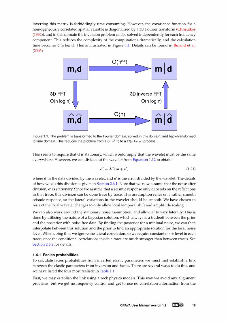
inverting this matrix is forbiddingly time consuming. However, the covariance function for ahomogeneously correlated spatial variable is diagonalised by a 3D Fourier transform (Christakos(1992)), and in this domain the inversion problem can be solved independently for each frequencycomponent. This reduces the complexity of the computations dramatically, and the calculationtime becomes O(n log n). This is illustrated in Figure 1.1. Details can be found in Buland et al.(2003)

Figure 1.1. The problem is transformed to the Fourier domain, solved in this domain, and back-transformedto time domain. This reduces the problem from a O(n2.x) to a O(n log n) process.

This seems to require that d is stationary, which would imply that the wavelet must be the sameeverywhere. However, we can divide out the wavelet from Equation 1.12 to obtain

d′ = ADm + e′, (1.21)

where d′ is the data divided by the wavelet, and e′ is the error divided by the wavelet. The detailsof how we do this division is given in Section 2.6.1. Note that we now assume that the noise afterdivision, e′ is stationary. Since we assume that a seismic response only depends on the reflectionsin that trace, this division can be done trace by trace. This assumption relies on a rather smoothseismic response, so the lateral variations in the wavelet should be smooth. We have chosen torestrict the local wavelet changes to only allow local temporal shift and amplitude scaling.

We can also work around the stationary noise assumption, and allow e′ to vary laterally. This isdone by utilising the nature of a Bayesian solution, which always is a tradeoff between the priorand the posterior with noise free data. By finding the posterior for a minimal noise, we can theninterpolate between this solution and the prior to find an appropriate solution for the local noiselevel. When doing this, we ignore the lateral correlation, so we require constant noise level in eachtrace, since the conditional correlations inside a trace are much stronger than between traces. SeeSection 2.6.2 for details.

1.4.1 Facies probabilitiesTo calculate facies probabilities from inverted elastic parameters we must first establish a linkbetween the elastic parameters from inversion and facies. There are several ways to do this, andwe have listed the four most realistic in Table 1.1.

First, we may establish the link using a rock physics models. This way we avoid any alignmentproblems, but we get no frequency control and get to use no correlation information from the


Table 1.1. Different methods for establishing a relation between elastic parameters and facies.

Approach Frequency Inversion Alignment Predictionscontrol correlation

Rock physics No No Yes OptimisticLow-pass filtered elastic well logs Yes No Yes OptimisticInversion Yes Yes No PessimisticParameter filtered elastic well logs Yes Yes Yes Realistic

Figure 1.2. Acoustic impedance residuals calculated from blocked raw logs plotted against correspondingVp/Vs residuals (left), the same plot, but with logs high-cut frequency filtered to 40Hz (middle), and the samelogs but filtered using frequency and correlation information from inversion (right).

inversion. A prediction obtained this way tends to be too optimistic, but if there are no well logsavailable, this is our only option.

Second, we may filter the elastic well logs using a low-pass filter, and use these filtered logsand facies logs to make a density estimation of p(µm|dobs

|f), where f is the facies. This gives usfrequency control and proper alignment, but again there are no correlation information from theinversion included, and the predictions become to optimistic. The frequency filtering of well logsis illustrated in Figure 1.2.

Third, we may set up the probability density for an elastic responds given the facies directly fromthe inverted elastic parameters. This way we get both frequency control and correlation informa-tion included, but we get no alignment information, and the predictions become to pessimistic.

Finally, we may establish the density using elastic parameters from well logs, but filter theseusing frequency and correlation information obtained from the inversion. Since we only use welllogs to establish the density estimates, we get no alignment problems, and in total, this givesus realistic facies predictions. How the inversion-based filtering differs from the pure frequency-based filtering mentioned above is illustrated in Figure 1.2.

The link between facies and elastic parameters that we eventually are interested in is p(fi|µm|d,i),where fi is the facies at location i and µm|d,i is the inversion result at the same location. To estab-lish this link, we must first establish a link between the well logs m and the expectation given theseismic data µm|dobs

. We get this by combining Equation 1.13 and Equation 1.19:

µm|dobs= µm + ΣmGTΣ−1

d (dobs − µd)

= µm + ΣmGTΣ−1d (Gm + e−Gµm)

= µm + F(m− µm) + e∗, (1.22)


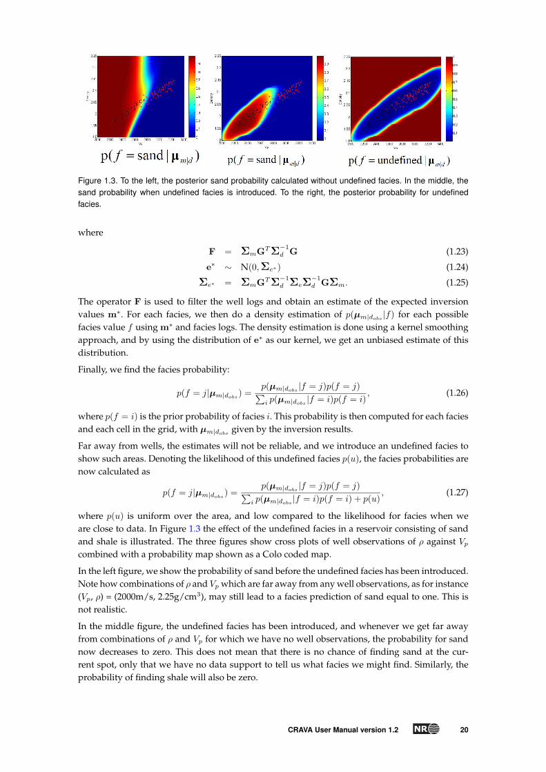
Figure 1.3. To the left, the posterior sand probability calculated without undefined facies. In the middle, thesand probability when undefined facies is introduced. To the right, the posterior probability for undefinedfacies.

where

F = ΣmGTΣ−1d G (1.23)

e∗ ∼ N(0,Σe∗) (1.24)

Σe∗ = ΣmGTΣ−1d ΣeΣ

−1d GΣm. (1.25)

The operator F is used to filter the well logs and obtain an estimate of the expected inversionvalues m∗. For each facies, we then do a density estimation of p(µm|dobs

|f) for each possiblefacies value f using m∗ and facies logs. The density estimation is done using a kernel smoothingapproach, and by using the distribution of e∗ as our kernel, we get an unbiased estimate of thisdistribution.

Finally, we find the facies probability:

p(f = j|µm|dobs) =

p(µm|dobs|f = j)p(f = j)∑

i p(µm|dobs|f = i)p(f = i)

, (1.26)

where p(f = i) is the prior probability of facies i. This probability is then computed for each faciesand each cell in the grid, with µm|dobs

given by the inversion results.

Far away from wells, the estimates will not be reliable, and we introduce an undefined facies toshow such areas. Denoting the likelihood of this undefined facies p(u), the facies probabilities arenow calculated as

p(f = j|µm|dobs) =

p(µm|dobs|f = j)p(f = j)∑

i p(µm|dobs|f = i)p(f = i) + p(u)

, (1.27)

where p(u) is uniform over the area, and low compared to the likelihood for facies when weare close to data. In Figure 1.3 the effect of the undefined facies in a reservoir consisting of sandand shale is illustrated. The three figures show cross plots of well observations of ρ against Vp

combined with a probability map shown as a Colo coded map.

In the left figure, we show the probability of sand before the undefined facies has been introduced.Note how combinations of ρ and Vp which are far away from any well observations, as for instance(Vp, ρ) = (2000m/s, 2.25g/cm3), may still lead to a facies prediction of sand equal to one. This isnot realistic.

In the middle figure, the undefined facies has been introduced, and whenever we get far awayfrom combinations of ρ and Vp for which we have no well observations, the probability for sandnow decreases to zero. This does not mean that there is no chance of finding sand at the cur-rent spot, only that we have no data support to tell us what facies we might find. Similarly, theprobability of finding shale will also be zero.


In the right figure, we show the probability of the undefined facies. This is zero around well obser-vations, and gradually increases to one as the distance to observations increase. The probabilityof shale may be extracted from these figures since p(sand) + p(shale) + p(undefined) = 1.


2 Implementation

Whereas the general model was explained in Chapter 1 we explain a bit more of the actual imple-mentation details here.

The estimation routines implemented in CRAVA are based on straightforward and commonlyused techniques. This gives fast and robust estimation, although we may run into problems if thenumber of data points is too small, or the data quality is too low. The quality of an estimationresult is never better than the quality of the data it is based on.

2.1 Estimating optimal well locationThe positioning uncertainty between well data and seismic data is often significant. To overcomethis, the well may be moved to the location with maximum correlation between the seismic dataand the reflection coefficients calculated from the well data. The relation between the seismicdata and reflection coefficients is linear; so linear covariance is a good measure. The optimal welllocation is found by searching for the location with highest covariance in a lateral neighbourhoodaround the original well location, where the well is allowed to be shifted vertically in each targetposition. The moving of wells is triggered by a command in the model file, and it is done prior tothe estimation of wavelets, noise, correlations and background model.

2.2 Estimating the prior modelThe prior model for the Bayesian inversion is defined in equation (1.10), and consists of the ex-pectations of the elastic parameters Vp, Vs, and ρ collected in the vector µm, and their spatialcorrelation structure collected in the covariance matrix Σm. These expectations and covariancesmust be given prior values before the inversion.

2.2.1 Background modelThe expectation µm is usually referred to as the background model. As the seismic data do notcontain information about low frequencies, a background model is built to set the appropriatelevels for the elastic parameters in the inversion volume. To identify this level, we can plot thefrequency content of the seismic traces in the available wells, and identify lowest frequency forwhich seismic data contains enough energy to carry information.

In Figure 2.1, we have plotted the frequency content in the seismic data in two different wells. Thegreen curve gives the frequency content in the near stack and the blue curve gives the frequencycontent in the far stack. These plots show that the seismic data contain little energy below 5–6Hz,and the purpose of the background model is to fill this void.

The estimation of the background model is made in two steps. First, we estimate a depth trend forthe entire volume, and then we interpolate well logs into this volume using kriging. The estima-tion will by default contain information up to 6Hz, but this high-cut limit can be adjusted usingthe <high-cut-background-modelling> keyword.

When identifying the depth trend, it is important that the wells are appropriately aligned. Thealignment is defined by the time interval surfaces specified as input, or alternatively, the correla-tion direction surface. It is important that the alignment reflects the correlation structure (deposi-


Figure 2.1. The frequency content of the seismic traces in two different wells. The frequency content of thenear and far stacks are shown as green and blue curves respectively.

Figure 2.2. Well logs aligned according to true time scale (left) and according to stratigraphic depth (right).

tion/compaction), and if the time surfaces are either eroding or on-lapped, one should considerspecifying the correlation direction separately using the <correlation-direction> keyword.

In Figure 2.2, we show two well logs aligned according to deposition and according to the truetime scale. Evidently, an incorrect trend will be identified if the true vertical depth is used. Thesize of the error will depend on the stratigraphy.

Assuming properly aligned wells, the trend extraction starts by calculating an average log valuefor each layer. This average is calculated for the Vp, Vs, and ρ well logs and is based on all avail-able wells. The estimation uses a piecewise linear regression, rather than the more straightforwardarithmetic mean or moving average, as these measures are sensitive to the amount of data avail-able. The piecewise regression has the additional advantage that it can give trend estimates alsooutside the interval for which we have data available.

For the linear regression we require a minimum of 10 data points behind each estimate. In addi-tion, we require that the minimum number of data points must also be at least 5*Nwells. This waywe ensure that data points from different time samples are always included. Alternatively, theregression would reduce to an arithmetic mean whenever there are 10 or more wells available. Ifwe enter a region with no data points available at all, the minimum requirements are doubled.


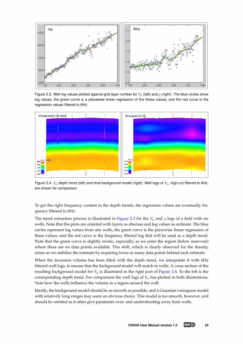
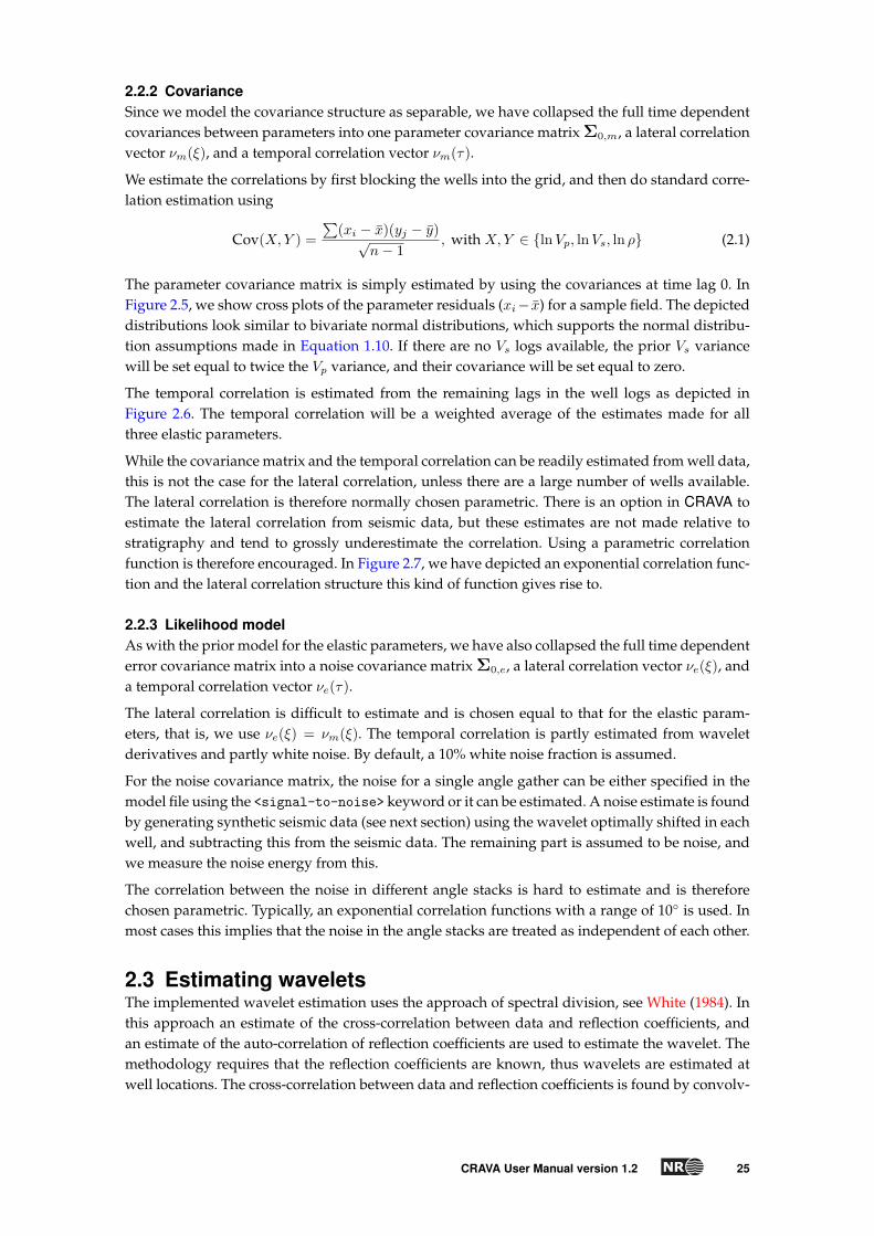
Figure 2.3. Well log values plotted against grid layer number for Vp (left) and ρ (right). The blue circles showlog values, the green curve is a piecewise linear regression of the these values, and the red curve is theregression values filtered to 6Hz.

Figure 2.4. Vp depth trend (left) and final background model (right). Well logs of Vp, high-cut filtered to 6Hz,are shown for comparison.

To get the right frequency content in the depth trends, the regression values are eventually fre-quency filtered to 6Hz.

The trend extraction process is illustrated in Figure 2.3 for the Vp and ρ logs of a field with sixwells. Note that the plots are oriented with layers as abscissa and log values as ordinate. The bluecircles represent log values from any wells, the green curve is the piecewise linear regression ofthese values, and the red curve is the frequency filtered log that will be used as a depth trend.Note that the green curve is slightly erratic, especially, as we enter the region (below reservoir)where there are no data points available. This shift, which is clearly observed for the density,arises as we stabilise the estimate by requiring twice as many data points behind each estimate.

When the inversion volume has been filled with the depth trend, we interpolate it with 6Hzfiltered well logs, to ensure that the background model will match in wells. A cross section of theresulting background model for Vp is illustrated in the right part of Figure 2.4. To the left is thecorresponding depth trend. For comparison the well logs of Vp has plotted in both illustrations.Note how the wells influence the volume in a region around the well.

Ideally, the background model should be as smooth as possible, and a Gaussian variogram modelwith relatively long ranges may seem an obvious choice. This model is too smooth, however, andshould be omitted as it often give parameter over- and undershooting away from wells.


2.2.2 CovarianceSince we model the covariance structure as separable, we have collapsed the full time dependentcovariances between parameters into one parameter covariance matrix Σ0,m, a lateral correlationvector νm(ξ), and a temporal correlation vector νm(τ).

We estimate the correlations by first blocking the wells into the grid, and then do standard corre-lation estimation using

Cov(X,Y ) =∑

(xi − x)(yj − y)√n− 1

, with X,Y ∈ {lnVp, lnVs, ln ρ} (2.1)

The parameter covariance matrix is simply estimated by using the covariances at time lag 0. InFigure 2.5, we show cross plots of the parameter residuals (xi− x) for a sample field. The depicteddistributions look similar to bivariate normal distributions, which supports the normal distribu-tion assumptions made in Equation 1.10. If there are no Vs logs available, the prior Vs variancewill be set equal to twice the Vp variance, and their covariance will be set equal to zero.

The temporal correlation is estimated from the remaining lags in the well logs as depicted inFigure 2.6. The temporal correlation will be a weighted average of the estimates made for allthree elastic parameters.

While the covariance matrix and the temporal correlation can be readily estimated from well data,this is not the case for the lateral correlation, unless there are a large number of wells available.The lateral correlation is therefore normally chosen parametric. There is an option in CRAVA toestimate the lateral correlation from seismic data, but these estimates are not made relative tostratigraphy and tend to grossly underestimate the correlation. Using a parametric correlationfunction is therefore encouraged. In Figure 2.7, we have depicted an exponential correlation func-tion and the lateral correlation structure this kind of function gives rise to.

2.2.3 Likelihood modelAs with the prior model for the elastic parameters, we have also collapsed the full time dependenterror covariance matrix into a noise covariance matrix Σ0,e, a lateral correlation vector νe(ξ), anda temporal correlation vector νe(τ).

The lateral correlation is difficult to estimate and is chosen equal to that for the elastic param-eters, that is, we use νe(ξ) = νm(ξ). The temporal correlation is partly estimated from waveletderivatives and partly white noise. By default, a 10% white noise fraction is assumed.

For the noise covariance matrix, the noise for a single angle gather can be either specified in themodel file using the <signal-to-noise> keyword or it can be estimated. A noise estimate is foundby generating synthetic seismic data (see next section) using the wavelet optimally shifted in eachwell, and subtracting this from the seismic data. The remaining part is assumed to be noise, andwe measure the noise energy from this.

The correlation between the noise in different angle stacks is hard to estimate and is thereforechosen parametric. Typically, an exponential correlation functions with a range of 10◦ is used. Inmost cases this implies that the noise in the angle stacks are treated as independent of each other.

2.3 Estimating waveletsThe implemented wavelet estimation uses the approach of spectral division, see White (1984). Inthis approach an estimate of the cross-correlation between data and reflection coefficients, andan estimate of the auto-correlation of reflection coefficients are used to estimate the wavelet. Themethodology requires that the reflection coefficients are known, thus wavelets are estimated atwell locations. The cross-correlation between data and reflection coefficients is found by convolv-


Figure 2.5. Cross plots of logarithmic parameter residuals. From such plots the parameter correlations maybe estimated.

Figure 2.6. We obtain the temporal covariance by measuring the covariance between all pairs of points inthe well log (left). The resulting temporal correlation function (right).

Figure 2.7. Parametric lateral correlations. A two-dimensional exponential correlation function (left). Thelateral correlation structure resulting from an anisotropic exponential correlation function having an azimuthof 45◦ degrees (right).


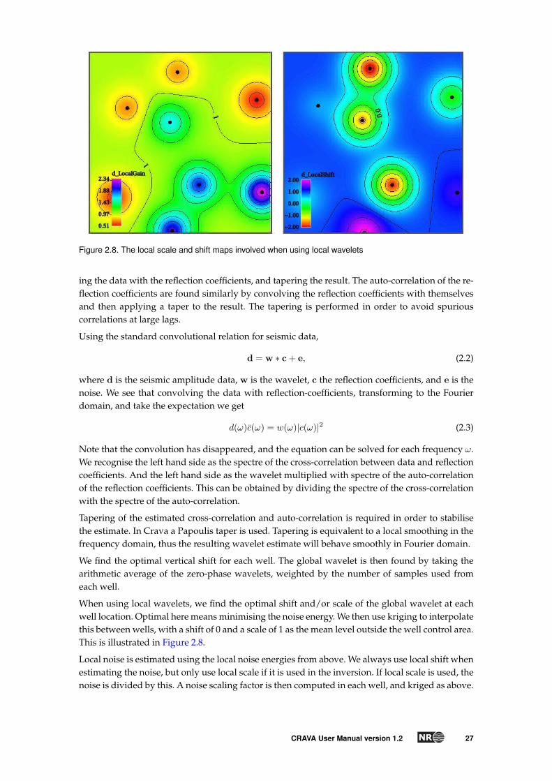
Figure 2.8. The local scale and shift maps involved when using local wavelets

ing the data with the reflection coefficients, and tapering the result. The auto-correlation of the re-flection coefficients are found similarly by convolving the reflection coefficients with themselvesand then applying a taper to the result. The tapering is performed in order to avoid spuriouscorrelations at large lags.

Using the standard convolutional relation for seismic data,

d = w ∗ c + e, (2.2)

where d is the seismic amplitude data, w is the wavelet, c the reflection coefficients, and e is thenoise. We see that convolving the data with reflection-coefficients, transforming to the Fourierdomain, and take the expectation we get

d(ω)c(ω) = w(ω)|c(ω)|2 (2.3)

Note that the convolution has disappeared, and the equation can be solved for each frequency ω.We recognise the left hand side as the spectre of the cross-correlation between data and reflectioncoefficients. And the left hand side as the wavelet multiplied with spectre of the auto-correlationof the reflection coefficients. This can be obtained by dividing the spectre of the cross-correlationwith the spectre of the auto-correlation.

Tapering of the estimated cross-correlation and auto-correlation is required in order to stabilisethe estimate. In Crava a Papoulis taper is used. Tapering is equivalent to a local smoothing in thefrequency domain, thus the resulting wavelet estimate will behave smoothly in Fourier domain.

We find the optimal vertical shift for each well. The global wavelet is then found by taking thearithmetic average of the zero-phase wavelets, weighted by the number of samples used fromeach well.

When using local wavelets, we find the optimal shift and/or scale of the global wavelet at eachwell location. Optimal here means minimising the noise energy. We then use kriging to interpolatethis between wells, with a shift of 0 and a scale of 1 as the mean level outside the well control area.This is illustrated in Figure 2.8.

Local noise is estimated using the local noise energies from above. We always use local shift whenestimating the noise, but only use local scale if it is used in the inversion. If local scale is used, thenoise is divided by this. A noise scaling factor is then computed in each well, and kriged as above.


2.4 Estimating 3D waveletThe expression for the wavenumber representation of the point-spread function given in Equa-tion 1.8 has only one unknown element, namely the 1D pulse w0(ω). The functions α1 and H aregiven as input, together with the average velocity V0. The elements needed for the conversionfrom depth to time are also input to CRAVA. That is the reference depth Z0, and reference timesurface T0. The theory for the estimation of the 1D pulse is given in Georgsen et al. (2010a), andwith more details in Georgsen et al. (2010b).

As for the 1D wavelet, the pulse is estimated from wells. Using reflection coefficients from welllogs, time gradients estimated from seismic data around wells and depth gradients computedfrom time gradients by using the reference time surface and average velocity given, a matrix Kcan be constructed forming a linear regression model for the seismic data as

d = Kw0 + e. (2.4)

The least squares estimate for w0 is

w0 = (K′K)−1G′d. (2.5)

2.5 Using FFT for inversionAs previously stated, Equation 1.12 separates when transformed into the Fourier domain. Afterthis transformation, the equation becomes

d(ω,k) = G(ω)m(ω,k) + e(ω,k)) (2.6)

The tilde denotes the 3D Fourier transform, with temporal frequency ω, and lateral frequencyvector k = (kx, ky). Due to the separation, we now have a set of n small equations, where nis the number of grid cells in the inversion volume. Everything is still normally distributed, sothe solution to this equation follows the pattern from Equation 1.19 and Equation 1.20. We stillmust invert a data covariance matrix, but whereas this matrix had dimension (n · nθ)2 before theFourier-transform, the matrix we must invert here is reduced to dimension n2

θ, where nθ is thenumber of angle stacks. Since the time for a matrix inversion is almost cubic in size, it is muchfaster to invert n of these small matrixes than the one large. After solving for m(ω,k), we do theinverse transform of this to obtain the distribution for m. The same does of course hold whenwe are using local wavelets that are divided out in advance, Equation 1.21. For full details, seeBuland et al. (2003).

2.6 A note one local wavelet and noiseAs shown, even though the use of FFT-transform requires stationarity, we are able to work aroundthis. Wavelets can be made local since these can be divided out before solving the equations, andlocally higher noise levels can be approximated by interpolating the low-noise solution and theprior distribution.

2.6.1 Local wavelet - dividing out the waveletA simple division of data by wavelet can easily be done in the Fourier domain, where the convo-lution reduces to a multiplication, and the division can be done one frequency at a time. However,this is very unstable for frequencies where the wavelet is very weak or not present, and some sortof stabilisation is needed.

In CRAVA this is done in two ways. First, we set an upper and lower cutoff frequency for thewavelet, default set to 5 and 55 Hz. Furthermore, for frequencies that fall below 10% of the averageamplitude, we set the amplitude to 10% of average before doing the division.


2.6.2 Local noiseLocal noise is implemented by first finding the solution using the minimum noise level, to fulfilthe stationarity requirements of the FFT algorithm. We then interpolate the values for each lo-cations between the prior and this minimum noise posterior. When doing this interpolation, weignore correlation between locations. This is not a problem as long as the noise varies slowly andsmoothly.

For each location x the adjusted estimate µm|dobs(x), is found from the inversion result µm|dobs

(x)by a linear relation,

µm|dobs(x) = µm(x) + Hx

(µm|dobs

(x)− µm(x)), (2.7)

The matrix Hx is a shrinkage matrix, i.e. the adjusted estimate is always closer to the prior meanthan the inversion result. The matrix Hx depends on the local error variance Σx

e and error vari-ance used in the inversion Σ0

e.

To find the shrinkage matrix we first identify a matrix G0 which maps the local prior distributionto the local posterior distribution when it is observed with the noise Σ0

e, that is,

d(x) = G0m(x) + e0,

where e0 ∼ N(0,Σ0

e

). The inversion of this expression is a linear relation

µm|dobs= µm + P(Σ0

e) (dobs − µd) (2.8)

where P(Σ0e) = ΣmGT

0

(G0ΣmG0

T + Σ0e

)−1

.

We then define the shrinkage matrix to be:

Hx(Σxe ,Σ

0e) = P(Σx

e )P(Σ0e)

−1. (2.9)

This removes the effect of the standard inversion and add the effect of the locally adapted inver-sion. The matrix P(Σ0

e) is not invertible, but since the local noise always is larger than the noisein the inversion the product in expression 2.9 is always well defined.

2.7 Memory handlingSince the grids needed by CRAVA can become very large, we try to keep the number of gridskept simultaneously in memory as small as possible. This implies that some allocated grids willbe used for more than one purpose. Both padded and unpadded grids are used in CRAVA, Theamount of memory needed by padded and unpadded grids are denoted sp and su respectively.

CRAVA also has an option to use disk space for intermediate storage of grids. This will reducethe memory consumption with a factor of at least 2 in realistic cases, but will also increase thecomputation time by a factor of almost 3.

2.7.1 Grid allocation with all grids in memoryIf intermediate disk storage is not used, the grid memory allocation will go as follows:

1. Background grids for Vp, Vs and density, 3 grids.

2. If the background model is to be estimated, another 3 grids are allocated for estimation, butdestroyed before any other allocations.

3. Seismic grids, nθ. If well optimisation is used, this will come before background grids.

4. Possibly prior facies probability grids, indicated by Ip, nf unpadded grids.


5. Prior covariance, 6 grids.

6. If relative facies probabilities or local noise, a copy of background indicated by Ib, 3 grids.

7. Peak: At this stage, CRAVA reaches its first memory peak. Minimum memory in use is 10grids, typical situation with three seismic grids and facies modelling requires 15 grids.Memory usage: P1 = (9 + nθ + Ib ∗ 3) ∗ sp + Ip ∗ nf ∗ su.

8. The posterior distribution is computed into the background and prior covariance grids, andseismic residuals are computed into the seismic grids. Thus, the inversion requires no extragrids. (But we needed a copy of the background for local noise or facies.)

9. After the inversion, the seismic grids are released, taking us off peak down to a base level:Memory usage: Pbase = (9 + Ib ∗ 3) ∗ sp + Ip ∗ nf ∗ su.

10. If simulation is used:

a. Simulated grids are allocated, 3 grids.

b. If secondary elastic parameters are requested as output (AI, µρ, etc.), indicated by Is, acomputation grid is allocated, 1 grid.

c. If kriging is used, indicated by Ik, 1 unpadded grid, not concurrent with computationgrid.

11. Peak: New possible peak, since the number of grids now allocated may be larger than thereleased seismic grids.Memory usage: P2 = (12 + Ib ∗ 3 + Is) ∗ sp + (Ip ∗ nf + max(0, Ik − Is)) ∗ su.

12. New release of grids, back to Pbase.

13. If facies probabilities:

a. 3D histograms of elastic parameters per facies are created, each of size 2MB, nf specialgrids.

b. Facies probability grids are created, including for undefined, nf + 1 unpadded grids.

14. Peak: New possible peak, since the new memory allocated may be larger than the releasedseismic grids and/or the simulation+computation/kriging grids.Memory usage: P3 = (9 + Ib ∗ 3) ∗ sp + (Ip ∗ nf + nf + 1) ∗ su + 2 ∗ nf .

15. Can now release all grids related to facies probability, memory down to 9 ∗ sp.

16. Eventual kriging of prediction allocates 1 unpadded grid.

17. Everything released.

The maximum memory usage is thus the largest of the actual peaks. The maximum number ofallocated padded grids will occur at either P1 or P2, whereas the largest number of other gridsare allocated at P3.


3 User guide

In this chapter, we describe how to build a CRAVA model file. The model file mainly follows theXML format, but we also use the character ’#’ for commenting, meaning that the rest of the lineafter such a character is read as comment. XML files are built with start and end tags, encapsulat-ing either tags or values. All model files start with <crava>, and end with </crava>. An exampleof a model file is given in Appendix A.

3.1 Basic inversionA primary ability for CRAVA is to run simple first-pass inversions. In this section, we describe howto build a model file for a simple inversion. We focus on how to get the key information into theprogram, whereas more detailed controls are discussed later, in Section 3.2. The key informationelements for a CRAVA inversion run is:

• Seismic data.

• Wavelet.

• Signal/noise ratio.

• Inversion volume.

• Background model.

• Correlation structures.

Since CRAVA is designed to estimate any information that is not given, well data must also com-monly be included.

3.1.1 Survey informationAll information regarding the seismic data is gathered under the <survey> tag. This includesthe file names for seismic data files, wavelet information and signal-to-noise ratio for each anglegather. As an example, it may look like this:

<crava>

<survey>

<segy-start-time> 2500.0 </segy-start-time>

<angle-gather>

<offset-angle> 16.0 </offset-angle>

<seismic-data>

<file-name> seismic/Cube16.segy </file-name>

</seismic-data>

</angle-gather>

<angle-gather>


<seismic-data>



</seismic-data>

</angle-gather>

</survey>

</crava>

The seismic data can be given on SegY-format, with a common offset time specified by the key-word <segy-start-time> if the offset is different from 0. The first value is used to represent theinterval from start-time to start-time + time-step, so with a start-time of 100ms, and 4ms sam-pling, the first value is used in the grid cell covering the interval 100-104ms. If we use seismicdata of another format than SegY, the <segy-start-time> command is not used. The file formatis detected automatically by CRAVA.

For each available angle, the rest of the information is gathered under an <angle-gather> tag,one for each offset. The actual angle is given by <offset-angle>.

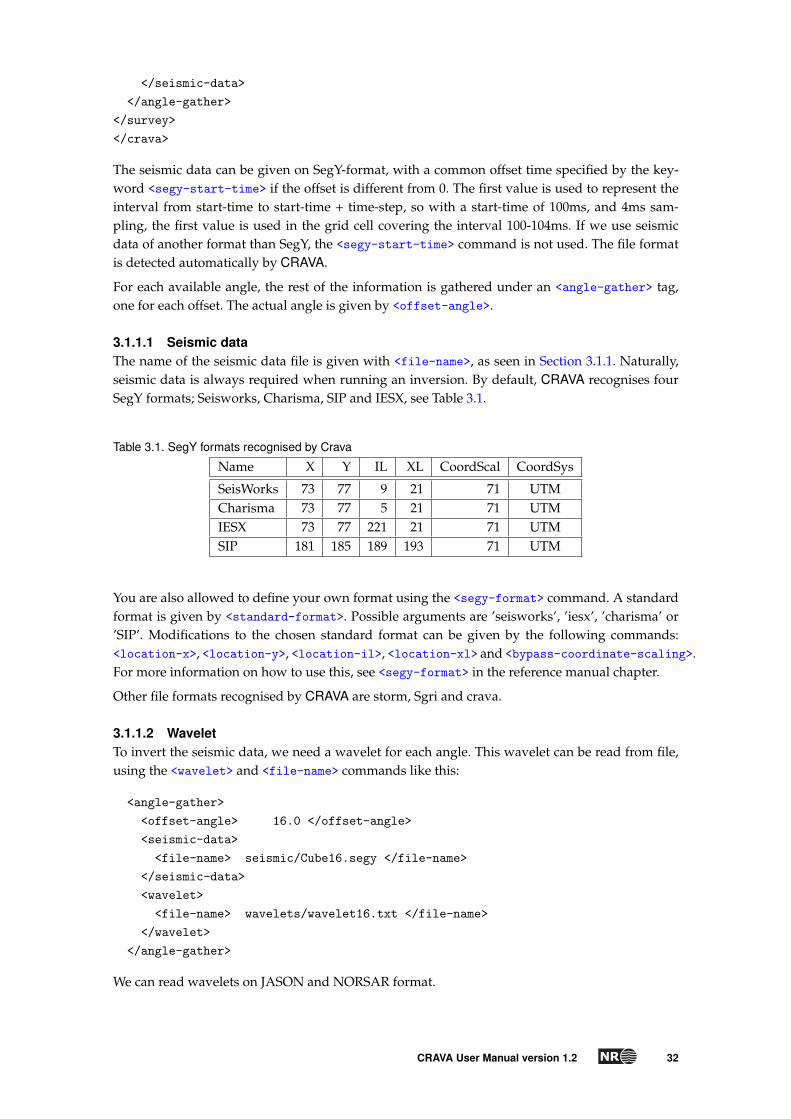
3.1.1.1 Seismic dataThe name of the seismic data file is given with <file-name>, as seen in Section 3.1.1. Naturally,seismic data is always required when running an inversion. By default, CRAVA recognises fourSegY formats; Seisworks, Charisma, SIP and IESX, see Table 3.1.

Table 3.1. SegY formats recognised by Crava

Name X Y IL XL CoordScal CoordSys

SeisWorks 73 77 9 21 71 UTMCharisma 73 77 5 21 71 UTMIESX 73 77 221 21 71 UTMSIP 181 185 189 193 71 UTM

You are also allowed to define your own format using the <segy-format> command. A standardformat is given by <standard-format>. Possible arguments are ’seisworks’, ’iesx’, ’charisma’ or’SIP’. Modifications to the chosen standard format can be given by the following commands:<location-x>, <location-y>, <location-il>, <location-xl> and <bypass-coordinate-scaling>.For more information on how to use this, see <segy-format> in the reference manual chapter.

Other file formats recognised by CRAVA are storm, Sgri and crava.

3.1.1.2 WaveletTo invert the seismic data, we need a wavelet for each angle. This wavelet can be read from file,using the <wavelet> and <file-name> commands like this:

<angle-gather>


<seismic-data>


</seismic-data>

<wavelet>

<file-name> wavelets/wavelet16.txt </file-name>

</wavelet>

</angle-gather>

We can read wavelets on JASON and NORSAR format.


The Ricker wavelet is implemented in CRAVA, and can be used by the command <ricker>. Thepeak frequency is given as argument.

If the <wavelet> command is not given, or given without <file-name>, the wavelet is estimated.See Section 2.3 for how this is done. If the wavelet is given on file, but not scaled, the command<scale> should be used if the scale is known, otherwise, the scale can be estimated by using the<estimate-scale> command. If none of these are specified, the wavelet will be used as it is onfile.

3.1.1.3 Signal/noise ratioThis ratio is given with <signal-to-noise-ratio>. If this command is not given, the ratio isestimated. Note that we define the signal to noise ratio as the data variance divided by the errorvariance, where the data variance is model variance plus error variance.

3.1.2 Inversion volumeThe volume used for inversion is given horizontally by a rectangle, and vertically bounded by atop and base surface. It is defined by the command <output-volume> under <project-settings>.Typically, it may look something like this:

<crava>

<project-settings>

<output-volume>

<utm-coordinates>

<reference-point-x> 403050.0 </reference-point-x>

<reference-point-y> 7211900.0 </reference-point-y>

<length-x> 500.0 </length-x>

<length-y> 500.0 </length-y>

<angle> 23.627 </angle>

<sample-density-x> 50.0 </sample-density-x>

<sample-density-y> 50.0 </sample-density-y>

</utm-coordinates>

<interval-two-surfaces>

<top-surface>

<time-file> horizons/FlatTop_3100ms.storm </time-file>

</top-surface>

<base-surface>

<time-file> horizons/FlatBase_3600ms.storm </time-file>

</base-surface>

<number-of-layers> 125 </number-of-layers>

</interval-two-surfaces>

</output-volume>

</project-settings>

</crava>

3.1.2.1 Lateral extentThe lateral extent of the inversion volume is specified by the command <area-from-surface>,<utm-coordinates>, or <inline-crossline-numbers>. The command <utm-coordinates> de-scribes a rectangle, which may be rotated relative to the seismic data. It has the following param-eters, which must all be specified:


• <reference-point-x> is the UTM x-coordinate of one corner of the area.

• <reference-point-y> is the UTM y-coordinate of the same corner.

• <length-x> is the extent of the area along the local x-axis.

• <length-y> is the extent of the area along the local y-axis.

• <angle> is the angle between the direction of the UTM x-axis and the local x-axis. Positiveangles are counterclockwise.

• <sample-density-x> is the length of one grid cell along the local x-axis.

• <sample-density-y> is the length of one grid cell along the local y-axis.

If the grid has the same rotation as the SegY volume read as input, output SegY volumes will havecorrect in-lines and cross-lines. Otherwise, these numbers are just counting from the initial corner.The command <area-from-surface> contains only one parameter, <file-name>, the name of astorm surface file defining the lateral extent of the inversion volume. The last way to define the in-version area is by the command <inline-crossline-numbers>. By this command, the followingparameters can be used:

• <il-start> is the starting inline number.

• <il-end> is the ending inline number.

• <xl-start> is the starting crossline number.

• <xl-end> is the ending crossline number.

• <il-step> is the inline interval.

• <xl-step> is the crossline interval.

The parameters <il-start> and <xl-start> must be set if this command is used, the other pa-rameters are optional. If they are not given, the numbers are taken from the Segy file containingthe first seismic cube.

The area commands may be skipped altogether. The area will then be taken from the first inputseismic data file, and defined as the smallest rectangle that covers all traces.

3.1.2.2 Top and base surfacesThe vertical extent is normally given by a top and a base surface in time, under the command<interval-two-surfaces> , as shown in Section 3.1.2. The file name for the top surface is givenunder command <top-surface>, <time-file>, and the base surface is given similarly under<base-surface> , <time-file>. The file format is binary storm or ASCII Irap. Top and base timevalues for the inversion interval can be given as constants instead of files, by using the command<time-value>.

These surfaces also define the default lateral correlation direction for the elastic parameters, withthe correlation being parallel to the top surface at the top, and base surface at the base. Betweenthis, we create a top- and base-conform grid, so that the number of grid cells in each trace isconstant, although the interval thickness may vary. This is shown in part B of Figure 3.1. Theinversion may be unstable if the resolution varies too much in different traces, so we recommendthat no trace interval is larger than twice the shortest interval. The number of layers between topand base is given by the command <number-of-layers> .


Figure 3.1. The layer structure of a (A) parallel top and base, (B) top- and base-conform compaction grid (C)Uniform correlation structure in a cut grid (D) Compactional correlation structure in a cut grid.

By specifying a correlation surface, the correlation direction can be independent of the intervalsurfaces, see part C of Figure 3.1 and Section 3.1.3.2. If this is done, there are no restrictions on thedifferences in interval thickness.

The more flexible approach where a compactional correlation structure is specified independentof the interval of interest (see part D of Figure 3.1) is currently not implemented.

If only one surface is known, the command <interval-one-surface> can be used to invert aninterval with top and base parallel to this surface. See Section 4.2.1.2 in the reference guide formore details. Note that depth conversion and correlation surfaces will not be available in thismode, so the lateral correlation will be parallel to this surface, as illustrated in part A of Figure 3.1.

3.1.2.3 Depth conversionThe <output-volume> command is also where the depth conversion is specified. Additional in-formation for depth conversion has only to be given under <interval-two-surfaces>, since thelateral area is the same. To do a depth conversion, one of the following must be given:

• Reference surface in depth (either top or base), and a velocity cube.

• Both top and base surface in depth. In this case, we assume constant velocity along each trace,computed from the time and depth surfaces.

• Both top and base surface in depth, and a velocity cube. In this case, we use the cube forrelative velocity in a trace, and scale it to match the interval length.

Reference surfaces in depth are given with the tags <depth-file> under <top-surface> and/or<base-surface>. The velocity cube can be read from file with the command <velocity-field>.


Alternatively, the command <velocity-field-from-inversion> can be used to specify that Vp

from inversion should be used for velocity. With depth conversion, the <interval-two-surfaces>command may look like this:


<top-surface>

<time-file> FlatTop_3100ms.storm </time-file>

<depth-file> FlatTop_3100ms.storm </depth-file>

</top-surface>

<base-surface>

<time-file> FlatBase_3600ms.storm </time-file>

<depth-file> FlatBase_3800ms.storm </depth-file>

</base-surface>

<velocity-field> velocity.storm </velocity-field>



3.1.3 Prior modelSince seismic data only contain information about relative elastic parameters, the absolute levelneeds to be set with a background model. In a Bayesian inversion setting, the background modelis the prior expectation. We also need the prior covariance, which is given by the covariance of theparameters, the lateral correlation and the temporal correlation, as described in Section 1.4. In themodel file, all this is gathered under the <prior-model> command, which may look somethinglike this:

<crava>

<prior-model>

<background>

<vp-file> input/background/CravaBgVp.storm </vp-file>

<vs-file> input/background/CravaBgVs.storm </vs-file>

<density-file> input/background/CravaBgRho.storm </density-file>

</background>

<lateral-correlation>

<variogram-type> genexp </variogram-type>

<power> 1 </power>

<angle> 0 </angle>

<range> 2500 </range>

<subrange> 2500 </subrange>

</lateral-correlation>

</prior-model>

</crava>

3.1.3.1 Background modelThe background model is given under the <background> command. It can be given from file,using <vp-file>, <vs-file> and <density-file>. These files should either be on Storm, crava,Sgri or SegY format. Alternatively, constant values can be used for background model, specifiedwith <vp-constant>, <vs-constant> and <density-constant>. Any combinations of files andconstants are also accepted. If none of these are given, the background model will be estimated.


3.1.3.2 CovariancesAs shown in Section 1.4 the prior covariance structure for the elastic parameters consists of threeparts:

1. A 3x3 covariance matrix for point-wise covariance between the parameters. May be readfrom ASCII file using the command <parameter-correlation>.

2. A temporal correlation vector, length equal to number of layers in grid, nt. May be read fromASCII file using the command <temporal-correlation>.

3. A lateral correlation structure. May be given as a parametric variogram using the command<lateral-correlation>.

By default, the two first are estimated from well data, and the lateral correlation structure is set toa isotropic exponential variogram with range 1000. The reason for the latter choice is that this ishard to estimate, see Section 2.2.2 for details. The most common to override is the lateral correla-tion, where the variogram used for petro-physical modelling is a good choice.

3.1.4 Well dataUnless all information about wavelet, signal to noise and correlations are specified, well data areneeded for estimation. Wells are given with the command <well-data>, and may look like this:

<crava>

<well-data>

<log-names>

<time> TWT </time>

<dt> DT </dt>

<dts> DTS </dts>

<density> RHOB </density>

</log-names>

<well>

<file-name> input/logs/ed6406_3-3_cut.rms </file-name>

</well>

<well>


</well>

<well>


</well>

<well>

<file-name> input/logs/ed6506_12-S4H_cut.rms </file-name>

</well>

</well-data>

</crava>

There are two main elements here. The first is a well log interpretation, given by <log-names>,which tells CRAVA which headers to look for. The following logs are needed:

• Two way time log, specified with <time>.

• Vp log, either given by <vp> or <dt>. The latter is used for DT-logs.

• Vs log, either given by <vs> or <dts>. The latter is used for DTS-logs.


• Density log, given by <density>.

In addition, if facies probabilities are computed, a facies log is needed. This is specified with thetag <facies>.

The wells are given with the command <file-name> under <well>, which is given once for eachwell. The reason for this is that additional information may be given for each well. Well filesshould be on NORSAR or RMS-format.

Each well may be moved to its optimal location using <optimize-position> under <well>, tak-ing the arguments <angle> and <weight> which allow the user to assign different weights to thedifferent angle gathers for each well. The maximum allowed offset and vertical shift for movingwells is specified in <maximum-offset> and <maximum-shift> under <well-data>, with defaultvalues of 250 m and 11 ms, respectively.

The command <synthetic-vs-log> tells whether the Vs log is synthetic. If not specified, it willbe detected from rank correlation with Vp. The command <filter-elastic-logs> is used to domulti-parameter-filtering of the elastic logs in this well after the inversion.

3.1.5 I/O settingsTwo commands are used to specify the directory for input files. <top-directory> gives the work-ing directory for the model file. The command <input-directory> is used to specify directoryname for root directory for input files. The name is given relative to <top-directory>.

Under <advanced-settings>, the command <use-intermediate-disk-storage> can be used tolimit the memory usage when running large CRAVA jobs. A built-in smart-swap is then activated.The option has largest effect on Microsoft Windows.

Under <project-settings>, <io-settings> and <other-output>, the command <error-file>

writes all errors to a separate file, in addition to the log file. The command <task-file> writes alltasks to a separate file, in addition to the log file.

3.1.6 OutputOutput is controlled under <io-settings> under <project-settings>. Here, you may set theoutput directory using <output-directory>, and you may also specify a prefix for all outputfiles using <file-output-prefix>.

Except for the log file which is placed directly under the output directory, all files output by cravaare placed in sub-directories. These sub-directories are

output-directory / wells

/ background

/ wavelets

/ seismic

/ velocity

/ correlations

/ inversionresults

There are two main output formats: Grid output, controlled by <grid-output>, and well outputcontrolled by <well-output>. The output section may look something like this:

<crava>

<project-settings>

<io-settings>

<file-output-prefix> CRAVA_ </file-output-prefix>


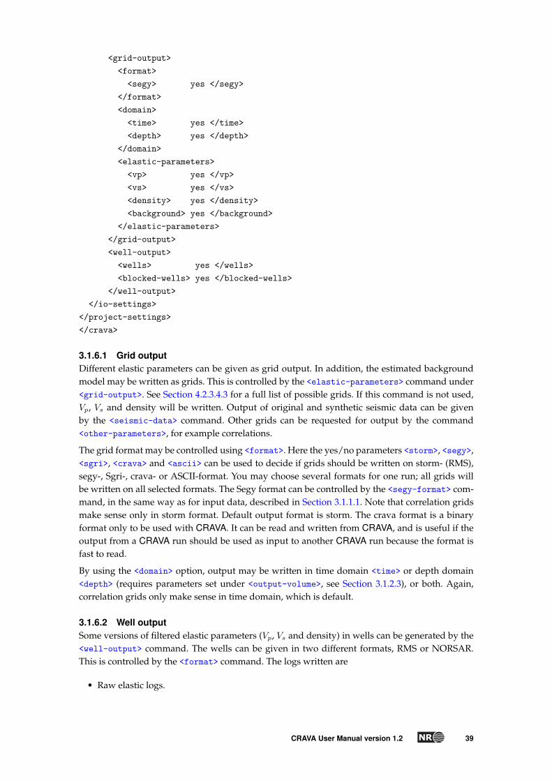
<grid-output>

<format>

<segy> yes </segy>

</format>

<domain>

<time> yes </time>

<depth> yes </depth>

</domain>

<elastic-parameters>

<vp> yes </vp>

<vs> yes </vs>

<density> yes </density>

<background> yes </background>

</elastic-parameters>

</grid-output>

<well-output>

<wells> yes </wells>

<blocked-wells> yes </blocked-wells>

</well-output>

</io-settings>

</project-settings>

</crava>

3.1.6.1 Grid outputDifferent elastic parameters can be given as grid output. In addition, the estimated backgroundmodel may be written as grids. This is controlled by the <elastic-parameters> command under<grid-output>. See Section 4.2.3.4.3 for a full list of possible grids. If this command is not used,Vp, Vs and density will be written. Output of original and synthetic seismic data can be givenby the <seismic-data> command. Other grids can be requested for output by the command<other-parameters>, for example correlations.

The grid format may be controlled using <format>. Here the yes/no parameters <storm>, <segy>,<sgri>, <crava> and <ascii> can be used to decide if grids should be written on storm- (RMS),segy-, Sgri-, crava- or ASCII-format. You may choose several formats for one run; all grids willbe written on all selected formats. The Segy format can be controlled by the <segy-format> com-mand, in the same way as for input data, described in Section 3.1.1.1. Note that correlation gridsmake sense only in storm format. Default output format is storm. The crava format is a binaryformat only to be used with CRAVA. It can be read and written from CRAVA, and is useful if theoutput from a CRAVA run should be used as input to another CRAVA run because the format isfast to read.

By using the <domain> option, output may be written in time domain <time> or depth domain<depth> (requires parameters set under <output-volume>, see Section 3.1.2.3), or both. Again,correlation grids only make sense in time domain, which is default.

3.1.6.2 Well outputSome versions of filtered elastic parameters (Vp, Vs and density) in wells can be generated by the<well-output> command. The wells can be given in two different formats, RMS or NORSAR.This is controlled by the <format> command. The logs written are

• Raw elastic logs.


• Elastic logs filtered to background frequency.

• Elastic logs filtered to seismic frequency.

• Elastic logs filtered with facies prediction filter (if available).

• Facies log (if available).

The wells can either be written with original sampling density, using <wells>, or matching theinternal grid resolution, using <blocked-wells>.

3.1.7 ActionsThe final information that is needed for a CRAVA run is what the run is supposed to do. This iscontrolled by <actions>. The <mode> keyword defines the purpose of this run and should be set to"inversion" when doing inversion. Other options are "estimation", see Section 3.3 and "forward",see Section 3.6. When inversion is chosen, <inversion-settings> can be used to control basicaspects of the inversion. It may look something like this:

<crava>

<actions>

<mode> inversion </mode>

<inversion-settings>

<prediction> yes </prediction>

<simulation>

<seed> 150570 </seed>

<number-of-simulations> 10 </number-of-simulations>

</simulation>

</inversion-settings>

</actions>

</crava>

The command <prediction> can be used to turn predictions on or off. By default, the predictionwill be generated. A number of full frequency stochastic realisations of the inversion can be ob-tained by specifying <number-of-simulations> under <simulation>. The seed for the randomgenerator can also be given here, with the <seed> command. Changing the seed will give a newset of realisations.

The command <kriging-to-wells> can be used to krige realisations to well data. By default, thisis done if the <simulation> command is used.

3.1.8 Standard grid formats• 3D-grid: Crava can read and write the following 3D grid formats: SegY, storm, Sgri (NOR-

SAR) and crava (internal) . On output, the format is controlled by a <format> keyword. Oninput, the program automatically detects the format, although it may need help to correctlyread SegY formats, using the <segy-format> keyword. The default output format is storm.

• Surfaces: The standard format for reading and writing surfaces is binary storm, but CRAVAcan also read Roxar ASCII surfaces (formerly known as ASCII Irap classic). In addition somesurfaces related to 3D-inversion are read as sgri (NORSAR). On input, the surface format willbe automatically detected.

• Wavelets: Wavelets are either on JASON or NORSAR format, both for reading and writing.Auto-detect is used on reading, use <format> for writing. The default output format is JA-SON.


• Wells: Wells are either on RMS or NORSAR format, both for reading and writing. Auto-detectis used on reading use <format> to control writing. The default output format is RMS.

3.2 Advanced inversion optionsAlthough CRAVA is mainly intended as a simple and fast inversion tool, there are still someoptions to control the inversion, and to access more sophisticated approaches. Most of these arecovered here, see also Section 4.2.4 for details about <advanced-settings>.

3.2.1 Non-stationary wavelet and noiseAlthough the FFT-algorithm which is at the core of CRAVA requires stationarity, this does notmean that the entire inversion has to be stationary, as discussed in Section 2.6. We allow lateralvariations in wavelet amplitude, wavelet shift and signal to noise ratio.

The local wavelet transformations fit well within the core framework of CRAVA, but the localnoise requires some approximations, as explained in section Section 2.6.2. This means that localnoise only improves the final result if the local variations are substantial. We do not recommendusing local noise if the variation in noise level is less than 15%.

Unlike the basic level, where parameters that were not specified automatically got estimated, theuse of local wavelets or local noise must be explicitly triggered. For wavelets, this is done withthe <local-wavelet> command under <wavelet>. There are four alternatives: <local-wavelet>:

1. <shift-file> gives a file name for a map giving the local shifts.

2. <estimate-shift> will estimate a local shift map when set to "yes".

3. <scale-file> gives a file name for a map giving the local scale.

4. <estimate-scale> will estimate a local scale map when set to "yes".

Naturally, the shift can not be both given and estimated, the same holds for scale. Note that youmay choose to use only shifts, omitting both scale keywords, or use only scale.

The local noise is triggered similarly, by using one of two commands under <angle-gather>:

1. <local-noise-scaled> gives a file name for a map with the local scaling of the signal tonoise ratio.

2. <estimate-local-noise> estimates the local scaling of the signal to noise ratio if set to "yes".

3.2.2 PS-seismic and reflection approximationsBy default, CRAVA assumes that the input seismic data are PP, but PS data can also be used.For both cases, we use the linearised Aki-Richards approximation, see Equation 1.1. The typeof seismic data is indicated by using the <type> command under<seismic-data>. Here, <type>should be either "pp" or "ps". Note that PS data must also be aligned in PP-travel time, as no suchalignment is done internally by CRAVA.

Instead of using the default reflection approximation, the user may supply the parameters tocompute the reflections. We always assume that for a given angle and seismic type, the reflectionscan be computed from the equation

c(x, t, θ) = aVp(θ)∂

∂tlnVp(x, t)

+ aVs(x, t, θ)∂

∂tlnVs(x, t)

+ aρ(x, t, θ)∂

∂tln ρ(x, t).

(3.1)


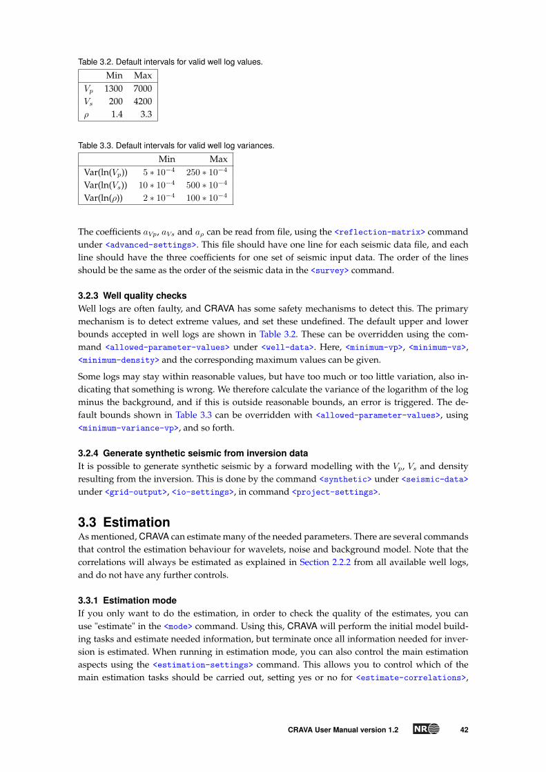
Table 3.2. Default intervals for valid well log values.

Min MaxVp 1300 7000Vs 200 4200ρ 1.4 3.3

Table 3.3. Default intervals for valid well log variances.

Min MaxVar(ln(Vp)) 5 ∗ 10−4 250 ∗ 10−4

Var(ln(Vs)) 10 ∗ 10−4 500 ∗ 10−4

Var(ln(ρ)) 2 ∗ 10−4 100 ∗ 10−4

The coefficients aVp, aVs and aρ can be read from file, using the <reflection-matrix> commandunder <advanced-settings>. This file should have one line for each seismic data file, and eachline should have the three coefficients for one set of seismic input data. The order of the linesshould be the same as the order of the seismic data in the <survey> command.

3.2.3 Well quality checksWell logs are often faulty, and CRAVA has some safety mechanisms to detect this. The primarymechanism is to detect extreme values, and set these undefined. The default upper and lowerbounds accepted in well logs are shown in Table 3.2. These can be overridden using the com-mand <allowed-parameter-values> under <well-data>. Here, <minimum-vp>, <minimum-vs>,<minimum-density> and the corresponding maximum values can be given.

Some logs may stay within reasonable values, but have too much or too little variation, also in-dicating that something is wrong. We therefore calculate the variance of the logarithm of the logminus the background, and if this is outside reasonable bounds, an error is triggered. The de-fault bounds shown in Table 3.3 can be overridden with <allowed-parameter-values>, using<minimum-variance-vp>, and so forth.

3.2.4 Generate synthetic seismic from inversion dataIt is possible to generate synthetic seismic by a forward modelling with the Vp, Vs and densityresulting from the inversion. This is done by the command <synthetic> under <seismic-data>under <grid-output>, <io-settings>, in command <project-settings>.

3.3 EstimationAs mentioned, CRAVA can estimate many of the needed parameters. There are several commandsthat control the estimation behaviour for wavelets, noise and background model. Note that thecorrelations will always be estimated as explained in Section 2.2.2 from all available well logs,and do not have any further controls.

3.3.1 Estimation modeIf you only want to do the estimation, in order to check the quality of the estimates, you canuse "estimate" in the <mode> command. Using this, CRAVA will perform the initial model build-ing tasks and estimate needed information, but terminate once all information needed for inver-sion is estimated. When running in estimation mode, you can also control the main estimationaspects using the <estimation-settings> command. This allows you to control which of themain estimation tasks should be carried out, setting yes or no for <estimate-correlations>,


<estimate-wavelet-or-noise> or <estimate-background>. Parameters with a "no" will not beestimated unless needed for other estimations. Note that in estimation mode, all estimated pa-rameters are written to file, regardless of output settings.

3.3.2 Wavelet and noise estimationWavelets and noise are estimated together. These parameters will only be estimated from wellsthat are vertical or close to vertical, since this allows comparing synthetic seismic from well logswith one or a couple of traces, and thus reduces alignment issues. The angle limit can be con-trolled by the <maximum-deviation-angle> command under <well-data>. In addition, wells canbe excluded individually, by setting <use-for-wavelet-estimation> to "no" under <well>.

By default, the wavelet and noise are estimated in the region between the top and base surface forthe inversion area. This may be limited using the <wavelet-estimation-interval> commandunder <survey>, where a separate set of restricting surfaces are given with <top-surface-file>

and <base-surface-file>. Since these are under <wavelet>, they can be different for each angle.

Some wavelet estimation options are also found under the command <advanced-settings> givenunder <project-settings>. These are

• <wavelet-tapering-length> which controls the length of the wavelet (in ms).

• <minimum-relative-wavelet-amplitude>which finds the wavelet length, by setting the cut-off size for edge peaks relative to centre peak.

• <maximum-wavelet-shift> which controls how far the wavelet can be shifted locally, seeSection 2.3.

Prior information for local wavelet modelling is given by the <local-wavelet> command under<prior-model>. Here, lateral correlation is specified as a 2D variogram for the lateral correlationin local wavelet modelling by the command <lateral-correlation>.

Output of wavelets is controlled by the <wavelet-output> command under <io-settings>. Twodifferent formats can be specified, JASON and NORSAR. Estimated wavelets for each well iswritten by the <well-wavelets> command. The command <global-wavelets> writes globalwavelets for each seismic angle. If local wavelet is requested, the command <local-wavelets>

writes estimated local wavelet shift and scale surfaces.

Output of estimated local noise surface is given by the command <local-noise> given under<io-settings> and <other-output>.

3.3.3 Background model estimationThe background model is estimated as a low frequency vertical trend. The trend is given in rela-tive depth in the inversion volume, so the trend value along the top and base surface is constant.At well locations, the trend is kriged to the well logs. By default, all wells are used for backgroundmodel estimation, but can be excluded by specifying "no" for <use-for-background-trend> un-der <well> for individual wells.

The background estimation can be controlled by some commands under <background>. Theseare:

• <velocity-field> takes an external velocity field, typically from migration, and uses as Vp

background, kriged to low frequency Vp well logs.

• <lateral-correlation> gives a variogram for the kriging. Larger ranges extends the influ-ence of well data further away from wells.


• <high-cut> allows specification of a maximum frequency for the background model.

3.3.4 Prior correlationsPrior correlations between Vp, Vs and density, and autocorrelation are estimated. they can be writ-ten to file by the command <prior-correlations> under <project-settings>, <io-settings>and <other-output>.

3.4 3D waveletInstead of the traditional 1D wavelet a 3D wavelet can be used in CRAVA. This wavelet is con-structed by a 1D pulse and a 3D wavelet filter based on illumination vectors. The use of a 3Dwavelet is invoked by the keyword <wavelet-3d>.

The 1D pulse used to construct the 3D wavelet, can be specified by the <file-name> keyword.If a file is not specified, this pulse is estimated. Either way, a filter file must be given by thekeyword <processing-factor-file-name>. This filter contains the amplitude effects related tothe illumination vectors and is given on Sgri format. One or two filters are given. The first, andnecessary, contains frequency-independent amplitude effects, while the second, if given, containsfrequency-dependent amplitude effects.

For noise estimation in the 3D wavelet setting, a propagation filter file is given by the keyword<propagation-factor-file-name>. At present, this is not used. The keyword <stretch-factor>

can be given, but is not used since the stretch factor is automatically calculated from the offsetangle.

When estimating the 1D pulse, seismic data from a neighbourhood of the well can be used. Thedistance from the well, specified in meters, that data are collected is given by the commands<estimation-range-x-direction> and <estimation-range-y-direction>. The default is thatonly data from the well position are used.

When 3D wavelet is used, certain parameters related to the mapping between time and depthare needed. This occurs since the illumination vectors relates to depth, while CRAVA works intime. These settings are given under keyword <time-to-depth-mapping-for-3d-wavelet> in<project-settings>. A reference depth for the target area must be specified under the key-word <reference-depth>. This depth represents a constant surface which in time normally willrefer to a variable surface due to varying velocity above this depth. This reference surface isgiven by <reference-time-surface> and can be given on Storm- or Sgri-format. The parame-ter <average-velocity> refers to the average velocity in the target area which is needed for theestimation of the pulse.

3.5 Facies predictionAn important feature in CRAVA is the ability to create facies probabilities. This requires that<mode> is set to "inversion", and is triggered by the <facies-probabilities> command under<inversion-settings>.

The facies probabilities are computed based on the inversion results and a distribution for in-version values given facies computed from filtered well logs, where the filter is defined by theinversion. See Section 1.4.1. Probability volumes will be computed for all facies seen in wells, andif the command <facies-probabilities-with-undef> is used, an additional undefined proba-bility cube is also generated, indicating areas where the inversion values are too far away fromwell data to make reliable predictions.

Except from the trigger in <inversion-settings>, all parameters related to facies probabilities


are given under <facies-probabilities> under <prior-model>. Here is an example:

<crava>

<prior-model>

<facies-probabilities>

<use-vs> yes </use-vs>

<use-prediction> yes </use-prediction>

<use-absolute-elastic-parameters> yes </use-absolute-elastic-parameters>

<estimation-interval>

<top-surface-file> input/horizons/facies_top.storm </top-surface-file>

<base-surface-file> input/horizons/facies_base.storm </base-surface-file>

</estimation-interval>

<prior-probabilities>

<facies>

<name> sand </name>

<probability> 0.4 </probability>

</facies>

<facies>

<name> shale </name>

<probability> 0.6 </probability>

</facies>

</prior-probabilities>

</facies-probabilities>

</prior-model>

</crava>

Figure 3.2. A sample facies probability estimation. The black curve gives the probability of sand in a wellcontaining sand (orange), shale (green) and crevasse (brown). In the left figure the well was not included inthe facies probability estimate whereas it was included in the right figure.


If <use-absolute-elastic-parameters> is set to ’yes’, facies probability is computed based oninverted parameters including background model. If the distribution for elastic parameters foreach facies is constant over the inversion volume, using absolute values is more stable. However,if there are trends in the elastic parameters, the relative values are more robust. The default is touse relative values.

The interval to use for facies probability calculations can be set with <estimation-interval>,similar to estimation interval for wavelets. Parallel to the wavelet case, wells may also be excludedusing the <use-for-facies-probabilities> command under <well>.

3.5.1 Prior probabilitiesIn order to get reliable probabilities, we need good prior probabilities. By default, CRAVA com-putes the average fraction of each facies in the relevant interval of the wells. This can be over-ridden using the <prior-probabilities> command, which allows specification of these. Notethat probabilities must be given for each facies. Probabilities can either be given globally, with<probability>, or as a full 3D trend, using <probability-cube>. The latter takes a grid file asargument, and the corresponding grid must cover the inversion volume. A prior value for unde-fined facies is set with the command <uncertainty-level>.

3.5.2 Output parametersFacies probabilities can be written to file by using the command <facies-probabilities> or<facies-probabilities-with-undef> given under <project-settings>, <io-settings>, <grid-output>and <other-parameters>. <facies-probabilities> gives probabilities for the existing faciesthat sum up to one. This is recommended for use in RMS. <facies-probabilities-with-undef>includes probability for undefined facies, and this cube will be the most correct one. <facies-likelihood>writes the likelihood for inverted seismic for each facies, p(m|f), while <seismic-quality-grid>writes a grid kriged from values for fit between facies probabilities and facies observed in each ofthe wells.

Rock physics distributions can be written by the command <rock-physics-distributions> un-der <io-settings> and <other-output>. The distributions are written per facies, in a STORMgrid with Vp, Vs and density as axes.

3.6 Forward modellingA minor functionality in CRAVA is that it can do forward modelling, showing what seismic re-sponse the program would expect from a given set of elastic parameters. This is triggered by using"forward" as <mode>. In this mode, we generate synthetic seismic data from the given backgroundvolumes. A file for forward modelling looks like this:

<crava>

<actions>

<mode> forward </mode>

</actions>

<survey>

<angle-gather>

<offset-angle> 0 </offset-angle>

<wavelet>

<file-name> wavelets/ricker.txt </file-name>

</wavelet>


</angle-gather>

<angle-gather>


<wavelet>

<file-name> wavelets/rickershift.txt </file-name>

</wavelet>

</angle-gather>

</survey>

<prior-model>

<earth-model>

<vp-file> background/Vp.storm </vp-file>

<vs-file> background/Vs.storm </vs-file>

<density-file> background/Rho.storm </density-file>

</earth-model>

</prior-model>

<project-settings>

<output-volume>




<top-surface>

<time-file> horizons/top.irap </time-file>

</top-surface>

<base-surface>

<time-file> horizons/base.irap </time-file>

</base-surface>



</output-volume>

<io-settings>

<grid-output>

<format>

<segy> yes </segy>

</format>

</grid-output>

</io-settings>

</project-settings>

</crava>

Note that no seismic files are given under <survey>, as these are now computed. No wells areused, since nothing can be estimated here. We need the angles to generate seismic data for, thecorresponding wavelets, the elastic parameters (given as earth model), and the volume. Insteadof using one of the commands defining volume, the volume can be taken from Vp. The outputformat can be controlled using <io-settings>, as can input- and output-directory. Other inputwill be ignored.

4 Model file reference manual

The numbering shows the command grouping. A command with no sub-numbering expects avalue to be given, otherwise, it is only a grouping of other commands.

File names are currently given with a path relative to the directory settings in <project-settings>-<io-settings>-<input/output/top-directory>. If these are not given, the path will always be rela-tive to the working directory.

All commands are optional, unless otherwise stated. A necessary command under an optional isonly necessary if the optional is given.

Standard grid formats for surfaces and 3D grids are given in Section 3.1.8.

4.1 <actions> (necessary)Description: Controls the main purpose of the run.Argument: Elements specifying the main purpose

4.1.1 <mode> (necessary)Description: Inversion: Invert seismic input data to elastic parameters and/or facies probabilities.

Needs seismic data and volume, all other missing data will be estimated. Forward: Createseismic response from background model. Not able to estimate anything. Estimation: Checksinput data and performs estimation of lacking information for inversion, but stops beforeinversion.

Argument: ’inversion’, ’forward’ or ’estimation’

4.1.2 <inversion-settings>

Description: Controls aspects of the inversion. Only valid with the <mode> ’inversion’ above.Argument: Elements controlling the inversionDefault:

4.1.2.1 <prediction>

Description: Controls whether predicted elastic parameters will be generated.Argument: ’yes’ or ’no’Default:

4.1.2.2 <simulation>

Description: Controls aspects of the simulation of elastic parameters.Argument: Elements controlling the simulation of elastic parameters

4.1.2.2.1 <seed>

Description: A number used to initialise the random generator. Running a model file with a givenseed will give the same simulation results each time.

Argument: IntegerDefault: 0


4.1.2.2.2 <seed-file>

Description: Alternative to <seed>. This is an ASCII file containing a number. At the terminationof the run, the file will be overwritten with a seed generated by the random generator. Thus,a model file using this will generate different simulation results on sequential runs.

Argument: ASCII file containing a numberDefault:

4.1.2.2.3 <number-of-simulations>

Description: Integer value giving the number of stochastic realizations to generate.Argument: IntegerDefault: 0

4.1.2.3 <kriging-to-wells>

Description: Should the realizations be kriged to well data?Argument: ’yes’ or ’no’Default: ’yes’ if not the <simulation> command is used.

4.1.2.4 <facies-probabilities>

Description: Should facies probabilities be estimated?Argument: ’yes’ or ’no’Default: ’no’

4.1.3 <estimation-settings>

Description: Controls what will be estimated. Only valid with the <mode> ’estimation’. Note thatthese commands can only turn off estimations - a parameter that is given will not be esti-mated even if it says so here.

Argument: Elements controlling what to estimateDefault:

4.1.3.1 <estimate-background>

Description: If ’no’, background will not be estimated unless needed for other estimation.Argument: ’yes’ or ’no’Default: ’yes’

4.1.3.2 <estimate-correlations>

Description: If ’no’, correlations will not be estimated unless needed for other estimation.Argument: ’yes’ or ’no’Default: ’yes’

4.1.3.3 <estimate-wavelet-or-noise>

Description: If ’no’, wavelets and/or noise will not be estimated unless needed for other estima-tion.

Argument: ’yes’ or ’no’Default: ’yes’

4.2 <project-settings> (necessary)Description: Controls inversion volume, output and advanced program settings.Argument: Elements controlling inversion volume, output and advanced program settings


Default:

4.2.1 <output-volume> (necessary)Description: Defines the core inversion volume. All grid output will be given in this volume.Argument: Elements defining the core inversion volume.Default:

4.2.1.1 <interval-two-surfaces>

Description: One way to give the top and bottom limitations. Must be used if output in depthdomain is desired. This or <interval-one-surface> must be given.

Argument:Default:

4.2.1.1.1 <top-surface> (necessary)

Description: File name(s) for top surface file(s).Argument: Elements controlling the top surfaceDefault:

4.2.1.1.1.1 <time-file>

Description: File name for standard surface file giving top surface in time. This or <time-value>must be given.

Argument: File nameDefault:

4.2.1.1.1.2 <time-value>

Description: Value giving the top time for the inversion interval. This or <time-file> must begiven.

Argument: ValueDefault:

4.2.1.1.1.3 <depth-file>

Description: File name for standard surface file giving top surface in depth.Argument: File nameDefault:

4.2.1.1.2 <base-surface> (necessary)

Description: File name(s) for base surface file(s).Argument: Elements controlling the base surfaceDefault:

4.2.1.1.2.1 <time-file>

Description: File name for standard surface file giving base surface in time. This or <time-value>must be given.



4.2.1.1.2.2 <time-value>

Description: Value giving the base time for the inversion interval. This or <time-file> must begiven.


4.2.1.1.2.3 <depth-file>

Description: File name for standard surface file giving base surface in depth.Argument: File nameDefault:

4.2.1.1.3 <number-of-layers>

Description: Integer value giving how many layers to use between top and base surface.Argument: IntegerDefault:

4.2.1.1.4 <velocity-field>

Description: File name for standard 3D grid file. Gives more detailed depth conversion informa-tion. Without this, constant velocity per trace is used. If only one depth surface is given, thisis used to compute the other. Otherwise, the depth interval will always match both surfaces,but the velocity field is scaled and used for internal depth computations. Can not be usedwith <velocity-field-from-inversion>.


4.2.1.1.5 <velocity-field-from-inversion>

Description: If given, velocity field from inversion is used for depth conversion. See <velocity-field>for details on how this is done. Can not be used with <velocity-field>.

Argument: ’yes’ or ’no’Default:

4.2.1.2 <interval-one-surface>

Description: Using this command gives parallel top and base of inversion interval. This or <interval-two-surfaces>must be given.

Argument: Elements for parallel top and base inversion intervalDefault:

4.2.1.2.1 <reference-surface>

Description: File name for standard surface file. The top and base surfaces for the inversion inter-val will be parallel to this.


4.2.1.2.2 <shift-to-interval-top>


Description: Value giving the distance from reference surface to top surface. This value is addedto the reference surface to create the top surface.


4.2.1.2.3 <thickness>

Description: Value giving the thickness of the inversion interval. This value is added to the topsurface to create the base surface.


4.2.1.2.4 <sample-density>

Description: Value giving the thickness of a layer in the inversion interval. The thickness shouldbe divisible by this value.


4.2.1.3 <area-from-surface>

Description: Inversion area can be defined by a surface. Then the name of the surface is given inthis command. Other ways to define inversion area are by the commands <utm-coordinates>or <inline-crossline-numbers>. If none of these commands are used, the area is defined bythe first seismic data file, or from Vp if we do forward modelling.

Argument:Default:

4.2.1.3.1 <file-name>

Description: File name for standard surface file.Argument: File nameDefault:

4.2.1.3.2 <snap-to-seismic-data>

Description: Find the smallest rectangular IL-XL box enclosing the entire surface and do the in-version using these IL-XL values. This allows a user to specify an inversion area in UTM andget the inversion volume aligned with seismic data.

Argument: ’yes’ or ’no’Default: ’no’

4.2.1.4 <utm-coordinates>

Description: Describe area by UTM coordinates.Argument:Default:

4.2.1.4.1 <reference-point-x>

Description: Value giving the x-coordinate of a corner of the area.Argument: ValueDefault:


4.2.1.4.2 <reference-point-y>

Description: Value giving the y-coordinate of a corner of the area.Argument: ValueDefault:

4.2.1.4.3 <length-x>

Description: Value giving the area length along the rotated x-axis.Argument: ValueDefault:

4.2.1.4.4 <length-y>

Description: Value giving the area length along the rotated y-axis.Argument: ValueDefault:

4.2.1.4.5 <sample-density-x>

Description: Cell size along the rotated x-axis.Argument: IntegerDefault:

4.2.1.4.6 <sample-density-y>

Description: Cell size along the rotated y-axis.Argument: IntegerDefault:

4.2.1.4.7 <angle>

Description: Orientation of the azimuth.Argument:Default:

4.2.1.4.8 <snap-to-seismic-data>

Description: Find the smallest rectangular IL-XL box enclosing the entire UTM specified areaand do the inversion using these IL-XL values. This allows a user to specify an inversionarea in UTM coordinates and get an inversion volume aligned with seismic data. Keywords<sample-density-x> and <sample-density-y> are not needed when snapping is activated.


4.2.1.5 <inline-crossline-numbers>

Description: Describe area by inline and crossline numbers. il-start and xl-start must be given ifthis command is used, the other variables are optional. The numbers which are not specifiedare taken from the SegY file containing seismic data. The command is only working if seismicdata are given on SegY format.

Argument:Default:


4.2.1.5.1 <il-start>

Description: Start value for inline.Argument:Default:

4.2.1.5.2 <il-end>

Description: End value for inline.Argument:Default:

4.2.1.5.3 <xl-start>

Description: Start value for crossline.Argument:Default:

4.2.1.5.4 <xl-end>

Description: End value for crossline.Argument:Default:

4.2.1.5.5 <il-step>

Description: Step value for inline.Argument:Default:

4.2.1.5.6 <xl-step>

Description: Step value for crossline.Argument:Default:

4.2.2 <time-to-depth-mapping-for-3d-wavelet>

Description: Defines the mapping between pseudo-depth and local time in the target area for 3Dwavelet.

Argument: Reference depth, velocity and time surface for mappingDefault:

4.2.2.1 <reference-depth>

Description: Holds the z-value for the reference depth for target areaArgument: Depth in meterDefault:

4.2.2.2 <average-velocity>

Description: Holds the average velocity in the target areaArgument: Velocity in meter/secondDefault:


4.2.2.3 <reference-time-surface>

Description: File name for the time surface corresponding to the reference depth. Standard surfaceformat.


4.2.3 <io-settings>

Description: Holds commands that deal with what output to give and where, and where to findinput.

Argument: Elements controlling output and inputDefault:

4.2.3.1 <top-directory>

Description: Directory name giving the working directory for the model file. Must end with direc-tory separator.

Argument: Directory nameDefault:

4.2.3.2 <input-directory>

Description: Directory name, relative to <top-directory>, for root directory for input files. Mustend with directory separator.


4.2.3.3 <output-directory>

Description: Directory name, relative to <top-directory>, for root directory for output files. Mustend with directory separator.


4.2.3.4 <grid-output>

Description: All commands related to output given as grids are gathered here.Argument: Elements controlling output given as gridsDefault:

4.2.3.4.1 <domain>

Description: Commands specifying which domain output should be in.Argument: Elements controlling the output domainDefault:

4.2.3.4.1.1 <depth>

Description: Should output come in depth domain? Requires information under <interval-two-surfaces>.Argument: ’yes’ or ’no’Default: ’no’

4.2.3.4.1.2 <time>

Description: Should output come in time domain?


Argument: ’yes’ or ’no’Default: ’yes’

4.2.3.4.2 <format>

Description: Control of the format of output grids.Argument: Elements controlling the format of output gridsDefault:

4.2.3.4.2.1 <segy-format>

Description: Information about the segy format. By default CRAVA recognises SeisWorks, IESX,SIP and Charisma, see Table 3.1.

Argument: Elements containing information about the segy format.Default:

4.2.3.4.2.1.1 <standard-format>

Description: Giving the starting format for modifications.Argument: ’seisworks’, ’iesx’, ’charisma’ or ’SIP’Default: ’seisworks’

4.2.3.4.2.1.2 <location-x>

Description: The byte location for the x-coordinate in the trace header.Argument: IntegerDefault:

4.2.3.4.2.1.3 <location-y>

Description: The byte location for the y-coordinate in the trace header.Argument: IntegerDefault:

4.2.3.4.2.1.4 <location-il>

Description: The byte location for the inline in the trace header.Argument: IntegerDefault:

4.2.3.4.2.1.5 <location-xl>

Description: The byte location for the crossline in the trace header.Argument: IntegerDefault:

4.2.3.4.2.1.6 <bypass-coordinate-scaling>

Description: Indicates whether coordinate scaling information should be used.Argument: ’yes’ or ’no’Default:


4.2.3.4.2.1.7 <location-scaling-coefficient>

Description:Argument: IntegerDefault:

4.2.3.4.2.2 <segy>

Description: Should grid output come as segy?Argument: ’yes’ or ’no’Default:

4.2.3.4.2.3 <storm>

Description: Should grid output come as storm?Argument: ’yes’ or ’no’Default: ’yes’ if <format> command is not given.

4.2.3.4.2.4 <crava>

Description: Should grid output come in crava binary format?Argument: ’yes’ or ’no’Default:

4.2.3.4.2.5 <sgri>

Description: Should grid output come as storm sgri?Argument: ’yes’ or ’no’Default:

4.2.3.4.2.6 <ascii>

Description: Should grid output come as storm ascii?Argument: ’yes’ or ’no’Default:

4.2.3.4.3 <elastic-parameters>

Description: Controls which elastic grid parameters to output. All are ’yes’ or ’no’.Argument: Elements controlling which elastic parameters to outputDefault: If this command is not given, vp, vs and density are written.

4.2.3.4.3.1 <vp>

Description:Argument: ’yes’ or ’no’Default:

4.2.3.4.3.2 <vs>



4.2.3.4.3.3 <density>


4.2.3.4.3.4 <lame-lambda>


4.2.3.4.3.5 <lame-mu>


4.2.3.4.3.6 <poisson-ratio>


4.2.3.4.3.7 <ai>


4.2.3.4.3.8 <si>


4.2.3.4.3.9 <vp-vs-ratio>


4.2.3.4.3.10 <murho>


4.2.3.4.3.11 <lambdarho>



4.2.3.4.3.12 <background>


4.2.3.4.3.13 <background-trend>


4.2.3.4.4 <seismic-data>

Description: Controls which seismic data parameters to output. All are ’yes’ or ’no’.Argument: Elements controlling which seismic data to outputDefault:

4.2.3.4.4.1 <original>

Description: Write original seismic data to file.Argument: ’yes’ or ’no’Default:

4.2.3.4.4.2 <synthetic>

Description: Generate synthetic seismic from the inverted data.Argument: ’yes’ or ’no’Default:

4.2.3.4.4.3 <residuals>

Description: Residuals computed in the actual inversion. Will not add up to original seismic datawhen combined with synthetic seismic, due to some filtering and numerical imprecision.


4.2.3.4.4.4 <synthetic-residuals>

Description: Residuals computed by taking the original seismic and subtracting the synthetic seis-mic. This means that these parameters are a matched set.


4.2.3.4.5 <other-parameters>

Description: Controls which other parameters to output. All are ’yes’ or ’no’.Argument: Elements controlling which other to outputDefault:

4.2.3.4.5.1 <facies-probabilities>

Description: Write facies probabilities to file.


Argument: ’yes’ or ’no’Default: ’yes’ if facies estimation is requested and <facies-probabilities-with-undef> is

not specified

4.2.3.4.5.2 <facies-probabilities-with-undef>

Description: Write facies probabilities with undefined value to file.Argument: ’yes’ or ’no’Default: ’no’

4.2.3.4.5.3 <facies-likelihood>

Description: Write likelihood for inverted seismic for each facies, p(m|f).Argument: ’yes’ or ’no’Default: ’no’

4.2.3.4.5.4 <time-to-depth-velocity>

Description: Write time-to-depth velocity to file.Argument: ’yes’ or ’no’Default:

4.2.3.4.5.5 <extra-grids>

Description: Temporary, will be replaced. Currently triggers writing of

• Estimated background files in extended versions (go above and below inversion vol-ume).

• Estimated background files in standard volume.


4.2.3.4.5.6 <correlations>

Description: These are the posterior correlations between vp, vs and density after inversion.Argument: ’yes’ or ’no’Default:

4.2.3.4.5.7 <seismic-quality-grid>

Description: Quality grid kriged from values for fit between facies probabilities and facies ob-served in each of the wells.


4.2.3.5 <well-output>

Description: Collects all output that can be given in well format. Wells contain logs for vp, vsand density, each of these in four versions: Raw, filtered to background frequency, filtered toseismic frequency and seismic resolution. In addition, the facies log is written if found.

Argument: Elements collecting output given in well formatDefault:


4.2.3.5.1 <format>

Description: Controls well formats used for output. Default is RMS.Argument: Elements controlling the formats used for outputDefault:

4.2.3.5.1.1 <rms>

Description: Controls if wells are written on RMS format.Argument: ’yes’ or ’no’Default:

4.2.3.5.1.2 <norsar>

Description: Controls if wells are written on NORSAR format.Argument: ’yes’ or ’no’Default:

4.2.3.5.2 <wells>

Description: Writes wells following original sampling density.Argument: ’yes’ or ’no’Default:

4.2.3.5.3 <blocked-wells>

Description: Writes wells sampled to internal grid resolution.Argument: ’yes’ or ’no’Default:

4.2.3.5.4 <blocked-logs>

Description: Not currently active.Argument:Default:

4.2.3.6 <wavelet-output>

Description: Collects all output that can be given for wavelets.Argument: Elements controlling wavelet outputDefault:

4.2.3.6.1 <format>

Description: Controls wavelet formats used for output. Default is JASON.Argument: Elements controlling the formats used for outputDefault:

4.2.3.6.1.1 <jason>

Description: Controls if wavelets are written on JASON form, being ’wlt’ format.Argument: ’yes’ or ’no’Default: ’yes’


4.2.3.6.1.2 <norsar>

Description: Controls if wavelets are written on NORSAR form, being ’swav’ format.Argument: ’yes’ or ’no’Default: ’no’

4.2.3.6.2 <well-wavelets>

Description: Writes estimated wavelets for each well used for wavelet estimation. Note: Thesewavelets are not optimally shifted, but aligned for easy comparison.


4.2.3.6.3 <global-wavelets>

Description: Writes global wavelets for each seismic angle.Argument: ’yes’ or ’no’Default: ’no’

4.2.3.6.4 <local-wavelets>

Description: Writes estimated local wavelet shift and scale surfaces. Can only be written when<local-wavelet> is requested.


4.2.3.7 <other-output>

Description: Controls output that is neither standard grid nor well.Argument: Elements controlling outputDefault:

4.2.3.7.1 <extra-surfaces>

Description: Temporary, will be replaced. Currently writes:

• Top and base surface for constant thickness interval used for log filtering and faciesprobabilities.

• Top and base surface for extended inversion interval computed from correlation surface.

• Top and base surface for background estimation interval (larger than inversion interval).


4.2.3.7.2 <prior-correlations>

Description: Write prior correlation files.Argument: ’yes’ or ’no’Default:

4.2.3.7.3 <background-trend-1d>

Description: Write the background trend as 1D curve.Argument: ’yes’ or ’no’


Default:

4.2.3.7.4 <local-noise>

Description: Writes estimated local noise surface. Can only be written when <local-noise-scaled>

or <estimate-local-noise> is requested.Argument: ’yes’ or ’no’Default:

4.2.3.7.5 <rock-physics-distributions>

Description: Writes rock physics distribution per facies, in a vp, vs, and density STORM-grid. Onlyavailable when facies probabilities are computed.


4.2.3.7.6 <error-file>

Description: Writes all errors to a separate file, in addition to the log file.Argument: ’yes’ or ’no’Default: ’no’

4.2.3.7.7 <task-file>

Description: Writes all tasks to a separate file, in addition to the log file.Argument: ’yes’ or ’no’Default: ’no’

4.2.3.8 <file-output-prefix>

Description: Common prefix added to all files written in the run. Identifies the run.Argument: StringDefault:

4.2.3.9 <log-level>

Description:Argument: String. Possible values are error, warning, low, medium, high.Default: Low

4.2.4 <advanced-settings>

Description: A collection of different commands that control advanced aspects of the programcontrol.

Argument: Commands controlling advanced aspects of the program controlDefault:

4.2.4.1 <fft-grid-padding>

Description: Controls the padding size, can be used to optimize memory or improve visual results.Padding should be at least one range laterally, and a wavelet length vertically to avoid edgeeffects.

Argument: Elements controlling the padding sizeDefault:


4.2.4.1.1 <x-fraction>

Description: Value telling how large the padding in the x-direction should be relative to the x-length.

Argument: ValueDefault: 0.0

4.2.4.1.2 <y-fraction>

Description: Value telling how large the padding in the x-direction should be relative to the y-length.


4.2.4.1.3 <z-fraction>

Description: Value telling how large the padding in the x-direction should be relative to the thick-ness.


4.2.4.2 <use-intermediate-disk-storage>

Description: When running under Windows with less physical memory than the program re-quires, this activates a built-in smart-swap. It is more efficient to use this smart-swappingthan the built-in windows paging system. Linux/Unix swap is so efficient that this optionhas little effect there. If you run Crava on a machine that you share with other users, it can bewise to use this if you know that Crava will need most of the memory.


4.2.4.3 <vp-vs-ratio>

Description: Value of Vp/Vs ratio used in reflection matrix. By default, the Vp/Vs ratio is esti-mated from the background model.

Argument: ValueDefault: Not set

4.2.4.4 <vp-vs-ratio-from-wells>

Description: If this command is given, the Vp/Vs ratio used in the reflection matrix will be esti-mated from well data. By default, the ratio is taken from the background model. If the key-word <wavelet-estimation-interval> has also been specified, the estimate will be limitedto that interval.


4.2.4.5 <maximum-relative-thickness-difference>

Description: Value giving the limit of how small the minimum interval thickness can be relative tomaximum. If this gets too low, the transformation to stationarity for the FFT-algorithm givesstrange results.

Argument: ValueDefault: Default is 0.5, which is acceptable. Slightly smaller seems to work as well.


4.2.4.6 <frequency-band>

Description: This command controls the frequency band of the inversion, so high and/or lowfrequencies can be filtered away. This ought to be done by the wavelet, but can be done here.

Argument: Elements controlling the frequency band of the inversionDefault:

4.2.4.6.1 <low-cut>

Description: Value setting the minimum frequency affected by the inversion.Argument: ValueDefault: 5.0

4.2.4.6.2 <high-cut>

Description: Value setting the maximum frequency affected by the inversion.Argument: ValueDefault: 55.0

4.2.4.7 <energy-threshold>

Description: If the energy in a trace falls below this threshold relative to the average, the trace isinterpolated from neighbours.


4.2.4.8 <wavelet-tapering-length>

Description: Value giving the length of the wavelet to be estimated in ms.Argument: ValueDefault: 200.0

4.2.4.9 <minimum-relative-wavelet-amplitude>

Description: Value giving the ratio between the smallest relevant amplitude and the largest am-plitude of peaks on an estimated wavelet. Edge peaks below this ratio are removed.


4.2.4.10 <maximum-wavelet-shift>

Description: Value controlling how much the wavelet is allowed to be shifted when doing estima-tion of wavelet or noise.


4.2.4.11 <minimum-sampling-density>

Description: Threshold value for minimum sampling density allowed.Argument: ValueDefault: 0.5 ms

4.2.4.12 <minimum-horizontal-resolution>

Description: Threshold value for minimum horizontal resolution allowed.Argument: ValueDefault: 5 m


4.2.4.13 <white-noise-component>

Description: In order to stabilise the inversion, we need to interpret some of the noise as white.This value controls the fraction.

Argument: Value between 0 and 1.Default: 0.1

4.2.4.14 <reflection-matrix>

Description: The file should be a 3 by number of seismic data cubes ascii matrix. The first column isthe factor used for vp for each cube setting (angle and ps/pp) when computing the reflectioncoefficients. The second and third are for vs and density.

Argument: File nameDefault: Linearised Aki-Richards.

4.2.4.15 <kriging-data-limit>

Description: Integer value giving the limit for the amount of well data used to krige each point. Ahigh value gives a smoother and more exact field, but takes more time.

Argument: IntegerDefault: 250

4.2.4.16 <debug-level>

Description: Gives debug messages and output. Not intended for use except on request by NR.Argument: Integer value 0, 1 or 2.Default: 0

4.2.4.17 <smooth-kriged-parameters>

Description: Tells whether we should smooth borders between kriging blocks or not.Argument: yes or noDefault: no

4.2.4.18 <rms-panel-mode>

Description: Disables some checks that are unnecessary when running from RMS.Argument: yes or noDefault: no

4.2.4.19 <guard-zone>

Description: Changes the amount of data that will be required outside the interval of interest.The guard zone contains data that will contribute to the inversion results in the interval ofinterest, and reducing the guard zone is therefore discouraged.

Argument: ValueDefault: 100ms

4.2.4.20 <3d-wavelet-tuning-factor>

Description: Allows tuning of the 3D wavelet estimation. A large value forces better fit of wavelet,while a smaller value gives smaller secondary peaks in wavelet.

Argument: ValueDefault: 50


4.2.4.21 <gradient-smoothing-range>

Description: Controls smoothing of the gradient used in 3D wavelet estimate and 3D inversion.This should be of the order of the horisontal extent of the 3D wavelet.


4.2.4.22 <estimate-well-gradient-from-seismic>

Description: If ’yes’, the well gradient used for 3D wavelet estimation is estimated from seismic.Otherwise this is taken from the correlation direction.

Argument: yes or noDefault: no

4.3 <survey> (necessary)Description: All information about the seismic data is collected here.Argument: Elements containing information about the seismic dataDefault:

4.3.1 <angular-correlation>

Description: 1D variogram. Gives the noise correlation between survey angles.Argument: 1D variogram, see Section 4.6.Default:

4.3.2 <segy-start-time>

Description: Global start time for segy cubes. This is used if no individual time is given for a segy-cube.


4.3.3 <angle-gather> (necessary)Description: Repeatable command, one for each seismic data cube.Argument: Elements containing information about the different seismic data cubesDefault:

4.3.3.1 <offset-angle> (necessary)Description: This is the angle for the seismic data cube.Argument: ValueDefault:

4.3.3.2 <seismic-data> (necessary)Description: Information about the seismic data cube.Argument: Elements containing information about the seismic data cubeDefault:

4.3.3.2.1 <file-name> (necessary)

Description: File name for the seismic data cube of one of the standard 3D formats, see Sec-tion 3.1.8. The file type will be automatically detected.



4.3.3.2.2 <start-time>

Description: Value giving the start time for this segy file.Argument: ValueDefault:

4.3.3.2.3 <segy-format>

Description: Information about the segy format. By default, CRAVA recognises SeisWorks, IESX,SIP and Charisma. See Table 3.1.

Argument: Elements containing information about the segy formatDefault:

4.3.3.2.3.1 <standard-format>

Description: Giving the starting format for modifications.Argument: ’seisworks’, ’iesx’, ’charisma’ or ’SIP’Default: ’seisworks’

4.3.3.2.3.2 <location-x>

Description: The byte location for the x-coordinate in the trace header.Argument: IntegerDefault:

4.3.3.2.3.3 <location-y>

Description: The byte location for the y-coordinate in the trace header.Argument: IntegerDefault:

4.3.3.2.3.4 <location-il>

Description: The byte location for the inline in the trace header.Argument: IntegerDefault:

4.3.3.2.3.5 <location-xl>

Description: The byte location for the crossline in the trace header.Argument: IntegerDefault:

4.3.3.2.3.6 <bypass-coordinate-scaling>

Description: Indicates whether coordinate scaling information should be used.Argument: ’yes’ or ’no’Default:

4.3.3.2.3.7 <location-scaling-coefficient>

Description:Argument: Integer


Default:

4.3.3.2.4 <type>

Description: Indicating the type of seismic data. Note that if both pp and ps cubes are used, thesemust be aligned.

Argument: ’pp’ or ’ps’Default: ’pp’

4.3.3.3 <wavelet>

Description: Information about the wavelet for this angle and seismic type. If not given, the waveletwill be estimated.

Argument: Elements containing information about the wavelet and seismic typeDefault:

4.3.3.3.1 <file-name>

Description: File name for wavelet file on JASON or NORSAR format. Can not be given togetherwith ricker. If neither file-name nor ricker is given, wavelet is estimated.


4.3.3.3.2 <ricker>

Description: Use Ricker wavelet. Can not be given together with file-name. If neither file-namenor ricker is given, wavelet is estimated.

Argument: Peak frequencyDefault:

4.3.3.3.3 <scale>

Description: Wavelet read from file or ricker wavelet is multiplied by this. Has no meaning whenwavelet is estimated.


4.3.3.3.4 <estimate-scale>

Description: Should global scale be estimated?Argument: ’yes’ or ’no’Default:

4.3.3.3.5 <local-wavelet>

Description: The amplitude and shift of the wavelet may be modified locally by 2D fields for shiftand scale values. This is handled here.

Argument: Elements modifying the amplitude and shift of the waveletDefault:

4.3.3.3.5.1 <shift-file>


Description: File name for standard surface file giving the local shift for the wavelet. Not allowedwhen wavelet is estimated.


4.3.3.3.5.2 <scale-file>

Description: File name for standard surface file giving local scale for the wavelet. Not allowedwhen wavelet is estimated.


4.3.3.3.5.3 <estimate-shift>

Description: Should a local shift be estimated? Not allowed with <shift-file>, but can be usedboth with given and estimated wavelet.


4.3.3.3.5.4 <estimate-scale>

Description: Should a local scale be estimated? Not allowed with <scale-file>, but can be usedboth with given and estimated wavelet.


4.3.3.4 <wavelet-3d>

Description: Information about the 3D-wavelet for this angle and seismic type. If not given, a 1D-wavelet is assumed.

Argument: Elements containing information about the 3D-waveletDefault:

4.3.3.4.1 <file-name>

Description: File name for the 1D-wavelet file. This 1D-wavelet will define the 3D-wavelet incombination with the filter given in <processing-factor-file-name>. If not given, the 1D-wavelet is estimated.


4.3.3.4.2 <processing-factor-file-name>

Description: File name for 3D-wavelet damping factor filter file. The 3D-wavelet is defined by the1D-wavelet and the filter. The 1D-wavelet is either given in <file-name> or estimated. Ineither case this filter file must be given.

Argument: File name for the amplitude scalings in the wavenumber filter.Default:

4.3.3.4.3 <propagation-factor-file-name>

Description: File name for 3D-wavelet correction filter file. This is used to set up the noise modelfor the 3D-wavelet.


Argument: File name for the correction factors in the wavenumber filter.Default:

4.3.3.4.4 <stretch-factor>

Description: Stretch factor for 3D-wavelet. The pulse is stretch with this factor.Argument: Value > 0.0Default: 1.0

4.3.3.4.5 <estimation-range-x-direction>

Description: Range for area around the well in x-direction where data are used in 3D waveletestimation.

Argument: Value >= 0.0Default: 0.0

4.3.3.4.6 <estimation-range-y-direction>

Description: Range for area around the well in y-direction where data are used in 3D waveletestimation.

Argument: Value >= 0.0Default: 0.0

4.3.3.5 <match-energies>

Description: If ’yes’, signal to noise ratio and wavelet scaling will be set to match model valueswith empirical values. Not a common estimator.


4.3.3.6 <signal-to-noise-ratio>

Description: Value for the signal to noise value. If not given, this will be estimated.Argument: ValueDefault:

4.3.3.7 <local-noise-scaled>

Description: Name of standard surface file with local noise.Argument: File nameDefault:

4.3.3.8 <estimate-local-noise>

Description: Can not say ’yes’ here if <local-noise-scaled> is given.Argument: ’yes’ or ’no’Default:

4.3.4 <wavelet-estimation-interval>

Description: Controls the time interval used for wavelet estimation by a top and base surface.Argument: Elements controlling the time interval used for wavelet estimationDefault: By default, estimation is done from all available seismic and well data.


4.3.4.1 <top-surface-file>

Description: File name for standard surface file giving the top of the time interval used for waveletestimation.


4.3.4.2 <base-surface-file>

Description: File name for standard surface file giving the base of the time interval used for waveletestimation.


4.3.5 <time-gradient-settings>

Description: The prior standard deviation of the gradients are given, as well as the minimumdistance for where gradient lines should not cross each other

Argument: The standard deviation and the minimum distanceDefault:

4.3.5.1 <distance>

Description: The minimum lateral distance for where the gradient lines should not cross. The dis-tance is equal for both x- and y-direction.

Argument: ValueDefault: 100 m

4.3.5.2 <sigma>

Description: The prior standard deviation of the gradient. Equal for both x- and y-gradientsArgument: ValueDefault: 1 ms/m

4.4 <well-data>Description: All information about the well data is collected here.Argument: Elements containing information about the well dataDefault:

4.4.1 <log-names>

Description: CRAVA needs to find the time, vp, vs, density and possibly facies logs. The name ofthese logs in the well files are given here.

Argument: Name of logsDefault:

4.4.1.1 <time>

Description: Name of the TWT logArgument: StringDefault:

4.4.1.2 <vp>

Description: Name of the vp log. May not be given if <dt> is given.Argument: String


Default:

4.4.1.3 <dt>

Description: Name of the inverse vp log. May not be given if <vp> is given.Argument: StringDefault:

4.4.1.4 <vs>

Description: Name of the vs log. May not be given if <dts> is given.Argument: StringDefault:

4.4.1.5 <dts>

Description: Name of the inverse vs log. May not be given if <vs> is given.Argument: StringDefault:

4.4.1.6 <density>

Description: Name of the density log.Argument: StringDefault:

4.4.1.7 <facies>

Description: Name of the facies log.Argument: StringDefault:

4.4.2 <well>

Description: Repeatable command, one for each well. Contains information about the wells.Argument: Elements containing information about the wellsDefault:

4.4.2.1 <file-name>

Description: File name for a well file. RMS or Norsar format.Argument: File nameDefault:

4.4.2.2 <use-for-wavelet-estimation>

Description: Should this well be used for wavelet estimation?Argument: ’yes’ or ’no’Default:

4.4.2.3 <use-for-background-trend>

Description: Should this well be used for background trend estimation?Argument: ’yes’ or ’no’Default:

4.4.2.4 <use-for-facies-probabilities>

Description: Should this well be used for facies probability estimation?



4.4.2.5 <synthetic-vs-log>

Description: Is the Vs log in this well synthetic? Will be detected from Vp correlation if not speci-fied here.


4.4.2.6 <filter-elastic-logs>

Description: Should we multi-parameter-filter the elastic logs in this well after the inversion?Argument: ’yes’ or ’no’Default:

4.4.2.7 <optimize-position>

Description: Repeatable command, one for each offset angle used for estimating optimised welllocation for this well.

Argument: Elements controlling optimisation of well locationDefault:

4.4.2.7.1 <angle>

Description: Offset angle used for estimating optimised well locationArgument: ValueDefault:

4.4.2.7.2 <weight>

Description: Weight of the offset angle given in <angle>


4.4.3 <high-cut-seismic-resolution>

Description: This frequency is used to filter wells down to seismic resolution. Only used to gener-ate output logs for QC.


4.4.4 <allowed-parameter-values>

Description: Sometimes there are faulty values in well logs. Here, trigger values for error detectioncan be controlled. These fall in two categories: Actual log values that are wrong, or logs thathave extremely low or high variance when the background model is subtracted.

Argument: Elements controlling trigger values for error detectionDefault:

4.4.4.1 <minimum-vp>

Description: Value for the smallest legal vp value.Argument: ValueDefault: 1300 m/s


4.4.4.2 <maximum-vp>

Description: Value for the largest legal vp value.Argument: ValueDefault: 7000 m/s

4.4.4.3 <minimum-vs>

Description: Value for the smallest legal vs value.Argument: ValueDefault: 200 m/s

4.4.4.4 <maximum-vs>

Description: Value for the largest legal vs value.Argument: ValueDefault: 4200 m/s

4.4.4.5 <minimum-density>

Description: Value for the smallest legal density value.Argument: ValueDefault: 1.4 g/cm3

4.4.4.6 <maximum-density>

Description: Value for the largest legal density value.Argument: ValueDefault: 3.3 g/cm3

4.4.4.7 <minimum-variance-vp>

Description: Value for the smallest legal variance in the vp log after the background is subtractedand logarithm is taken.


4.4.4.8 <maximum-variance-vp>

Description: Value for the largest legal variance in the vp log after the background is subtractedand logarithm is taken.


4.4.4.9 <minimum-variance-vs>

Description: Value for the smallest legal variance in the vs log after the background is subtractedand logarithm is taken.


4.4.4.10 <maximum-variance-vs>

Description: Value for the largest legal variance in the vs log after the background is subtractedand logarithm is taken.



4.4.4.11 <minimum-variance-density>

Description: Value for the smallest legal variance in the density log after the background is sub-tracted and logarithm is taken.


4.4.4.12 <maximum-variance-density>

Description: Value for the largest legal variance in the density log after the background is sub-tracted and logarithm is taken.


4.4.4.13 <minimum-vp-vs-ratio>

Description: Value for the smallest Vp/Vs-ratio regarded as likely.Argument: ValueDefault: 1.4

4.4.4.14 <maximum-vp-vs-ratio>

Description: Value for the largest Vp/Vs-ratio regarded as likely.Argument: ValueDefault: 3.0

4.4.5 <maximum-deviation-angle>

Description: Value for the maximum deviation angle of a well before it is excluded from estimationbased on vertical wells (such as wavelet and signal to noise).


4.4.6 <maximum-rank-correlation>

Description: If the correlation between vp and vs logs exceed this value, the vs log is consideredto be synthetic, and not counted as additional data in estimation.

Argument: Value close to, but less than 1.Default: 0.99

4.4.7 <maximum-merge-distance>

Description: Value giving the minimum distance in time between well log entries before they aremerged to one observation.


4.4.8 <maximum-offset>

Description: Value giving the maximum allowed offset for moving wells in meters.Argument: ValueDefault: 250

4.4.9 <maximum-shift>

Description: Value giving the maximum allowed vertical shift for moving wells.Argument: ValueDefault: 11.0


4.4.10 <well-move-data-interval>

Description: Defines an interval for estimation of facies probability given elastic parameters.Argument: Elements defining estimation intervalDefault: Everywhere facies and elastic logs are present.

4.4.10.1 <top-surface-file>

Description: File name for standard surface file giving the top of the estimation interval.Argument: File nameDefault:

4.4.10.2 <base-surface-file>

Description: File name for standard surface file giving the base of the estimation interval.Argument: File nameDefault:

4.5 <prior-model>Description: This command defines the prior model for elastic parameters and possibly also facies.Argument: Elements defining prior models for elastic parameters and faciesDefault:

4.5.1 <background>

Description: Contains information about the background model or how to estimate it. Note thateither all parameters must be given, or all must be estimated.

Argument: Elements containing information about the background modelDefault:

4.5.1.1 <ai-file>

Description: File name for 3D grid file, giving background AI. Can not be given together with<vp-file> or <vp-constant>.


4.5.1.2 <si-file>

Description: File name for 3D grid file, giving background SI. Can not be given together with<vs-file> or <vs-constant> or <vp-vs-ratio-file>.


4.5.1.3 <vp-vs-ratio-file>

Description: File name for 3D grid file, giving background Vp/Vs. Can not be given together with<vs-file> or <vs-constant>.


4.5.1.4 <vp-file>

Description: File name for 3D grid file, giving background vp. Can not be given together with<vp-constant>.

Argument: File name


Default:

4.5.1.5 <vs-file>

Description: File name for 3D grid file, giving background vs. Can not be given together with<vs-constant>.


4.5.1.6 <density-file>

Description: File name for 3D grid file, giving background density. Can not be given together with<density-constant>.


4.5.1.7 <vp-constant>

Description: Value, used for constant vp background. Can not be given together with <vp-file>.Argument: ValueDefault:

4.5.1.8 <vs-constant>

Description: Value, used for constant vs background. Can not be given together with <vs-file>.Argument: ValueDefault:

4.5.1.9 <density-constant>

Description: Value, used for constant density background. Can not be given together with <density-file>.Argument: ValueDefault:

4.5.1.10 <velocity-field>

Description: File name for 3D grid file giving a velocity field used as base for vp in backgroundestimation. Can not be used if the background parameters are given.


4.5.1.11 <lateral-correlation>

Description: 2D variogram for the lateral correlation in the elastic parameters in the estimatedbackground model, used for kriging of wells. Can not be used if the background parametersare given.

Argument: 2D variogram, see Section 4.6.Default:

4.5.1.12 <high-cut-background-modelling>

Description: Value giving the maximum frequency in the estimated background model. Can notbe used if the background parameters are given.

Argument: ValueDefault: 6.0 Hz


4.5.2 <earth-model>

Description: Contains inverted seismic data used for forward modelling.Argument: Vp, vs and rho used for forward modelling.Default:

4.5.2.1 <vp-file>

Description: File name for 3D grid file, giving vp.Argument: File nameDefault:

4.5.2.2 <vs-file>

Description: File name for 3D grid file, giving vs.Argument: File nameDefault:

4.5.2.3 <density-file>

Description: File name 3D grid file, giving density.Argument: File nameDefault:

4.5.2.4 <ai-file>

Description: File name for 3D grid file, giving AI. Can not be given together with <vp-file> .Argument: File nameDefault:

4.5.2.5 <si-file>

Description: File name for 3D grid file, giving SI. Can not be given together with <vs-file2> or<vp-vs-ratio-file2>.


4.5.2.6 <vp-vs-ratio-file>

Description: File name for 3D grid file, giving Vp/Vs. Can not be given together with <vs-file2>.Argument: File nameDefault:

4.5.3 <local-wavelet>

Description: Contains prior information for local wavelet modelling.Argument: Elements containing prior information for local wavelet estimation.Default:

4.5.3.1 <lateral-correlation>

Description: 2D variogram for the lateral correlation in local wavelet modelling.Argument: 2D variogram, see Section 4.6.Default:

4.5.4 <lateral-correlation>

Description: 2D variogram for the lateral correlation in the elastic parameters.Argument: 2D variogram, see Section 4.6.


Default:

4.5.5 <temporal-correlation>

Description: File name for the temporal correlation file. The file is an ascii file. Usually, this filecomes from an earlier run of CRAVA.


4.5.6 <parameter-correlation>

Description: File name for the parameter correlation file. The file is an ascii file, containing covari-ances between Vp, Vs and density. It is most common to use a file resulting from an earlierrun of CRAVA, and the file might look like this:

0.001171 0.000786 0.000046

0.000786 0.001810 -0.000395

0.000046 -0.000395 0.000530


4.5.7 <correlation-direction>

Description: File name for the standard surface file giving the correlation direction for the inver-sion.


4.5.8 <facies-probabilities>

Description: Commands controlling the generating of facies probabilities.Argument: Elements controlling facies probabilitiesDefault:

4.5.8.1 <use-vs>

Description: Decides whether Vs information is used when computing facies probabilities.Argument: ’yes’ or ’no’.Default: ’yes’.

4.5.8.2 <use-prediction>

Description: Decides whether sampled inversion logs are used when computing facies probabili-ties. If not, filtered logs are used.

Argument: ’yes’ or ’no’.Default: ’no’.

4.5.8.3 <use-absolute-elastic-parameters>

Description: Decides whether facies probabilities are generated based on absolute elastic parame-ters or elastic parameters minus trend (background model).


4.5.8.4 <estimation-interval>

Description: Defines an interval for estimation of facies probability given elastic parameters.


Argument: Elements defining estimation intervalDefault: Everywhere facies and elastic logs are present.

4.5.8.4.1 <top-surface-file>

Description: File name for standard surface file giving the top of the estimation interval.Argument: File nameDefault:

4.5.8.4.2 <base-surface-file>

Description: File name for standard surface file giving the base of the estimation interval.Argument: File nameDefault:

4.5.8.5 <prior-probabilities>

Description: Prior facies probabilities are given for all facies. Priors can be given as constant num-bers or 3D cubes. If this command is not given, prior distribution is estimated from wells.

Argument: Elements controlling facies probabilitiesDefault:

4.5.8.5.1 <facies>

Description: Repeatable command, one for each facies. All facies present in well logs must begiven.

Argument: Elements containing information about the faciesDefault:

4.5.8.5.1.1 <name>

Description: Name of facies.Argument: Facies nameDefault:

4.5.8.5.1.2 <probability>

Description: Probability for the facies given above. Either this command or <probability-cube>is given, same for all facies.

Argument: Real numbers between 0 and 1. Numbers for all facies must sum to one.Default:

4.5.8.5.1.3 <probability-cube>

Description: File name for 3D grid file containing prior facies probability for facies with namegiven above. Either this command or <probability> is given, same for all facies.


4.5.8.6 <uncertainty-level>

Description: Value defining how large the undefined probability will be when facies probabilitiesare computed. This value is scaled and used as likelihood for undefined when facies proba-bilities are computed.



4.6 VariogramThe variograms are given on the following form:

4.6.1 <variogram-type>

Description: Either ’genexp’ or ’spherical’ for general exponential or spherical variogram.Argument:Default:

4.6.2 <angle>

Description: Value for the azimuth direction. Only for 2D variograms.Argument:Default:

4.6.3 <range>

Description: Value for the range in the azimuth direction.Argument:Default:

4.6.4 <subrange>

Description: Value for the range normal to the azimuth direction. Only for 2D variograms.Argument:Default:

4.6.5 <power>

Description: Value between 1 and 2 for the power of the general exponential variogram. Not al-lowed for spherical variogram.

Argument:Default:

All angles are given as mathematical angles in degrees.


A Sample model file

<crava>

<actions>

<mode> inversion </mode>

<inversion-settings>

<prediction> yes </prediction>

</inversion-settings>

</actions>

<survey>

<angular-correlation>


<range> 10 </range>

<power> 1 </power>

</angular-correlation>

<segy-start-time> 2500 </segy-start-time>

<angle-gather>


<seismic-data>


</seismic-data>

</angle-gather>

<angle-gather>


<seismic-data>


</seismic-data>

</angle-gather>

</survey>

<well-data>

<log-names>

<time> TWT </time>

<dt> DT </dt>

<dts> DTS </dts>

<density> RHOB </density>

</log-names>

<well>

<file-name> logs/ed6406_3-3_cut.rms </file-name>

</well>

<well>


</well>

<well>


</well>

<well>

<file-name> logs/ed6506_12-S4H_cut.rms </file-name>

</well>

</well-data>

<prior-model>


<background>

<high-cut-background-modelling> 6 </high-cut-background-modelling>





<angle> 70 </angle>

<power> 1 </power>


</background>





<angle> 70 </angle>

<power> 1 </power>


</prior-model>

<project-settings>

<output-volume>

<utm-coordinates>

<reference-point-x> 398500 </reference-point-x>

<reference-point-y> 7210300 </reference-point-y>

<length-x> 4500 </length-x>

<length-y> 4500 </length-y>

<angle> 23.627 </angle>

<sample-density-x> 50 </sample-density-x>

<sample-density-y> 50 </sample-density-y>

</utm-coordinates>


<top-surface>

<time-file> horizons/TopTime_avg3100ms.storm </time-file>

<depth-file> horizons/TopTime_avg3100ms.storm </depth-file>

</top-surface>

<base-surface>

<time-file> horizons/BaseTime_avg3600ms.storm </time-file>

</base-surface>

<velocity-field-from-inversion> yes </velocity-field-from-inversion>



</output-volume>

<io-settings>

<log-level> high </log-level>

<top-directory> ../ </top-directory>

<input-directory> input/ </input-directory>

<output-directory> output/ </output-directory>

<grid-output>

<format>

<ascii> yes </ascii>

</format>


B Test suite overview

This appendix gives an overview of the features that are currently tested in the test suite.

Test \ Case number 1 2 3 4 5 6 7 8 9 10 11 12 13 14 15 16 17 18Mode

Forward xEstimation - 1D x xEstimation - 3D xInversion - prediction x x x x x x x x x x x x xInversion - simulation xInversion - kriging x x xInversion - facies prob. x x x x

SurveyAngle gathers 2 2 2 2 2 2 2 2 2 2 3 3 3 3 3 2 2 2Estimate global wavelet x x x x xEstimate global SN-ratio x x x x xEstimate local noise xEstimate local scale xEstimate local shift xWavelet estimation interval x

WellsNumber of wells 1 1 1 4 4 4 4 1 1 6 6 6 6 1 1 2 3Only synthetic Vs logs x x<use-for-facies-probabilities> x x<synthetic-vs-log> x<filter-elastic-logs> x x<optimize-position> x<allowed-parameter-values> x x x x

Prior modelEstimate covariance x x x x x x x xEstimate background x x x x x x xAnisotropic background mod x x x x xAnisotropic lateral corr x x x x x x x xCorrelation direction xVpVsRho filter x xVpRho filter xUse prediction (not filter) xAbsolute params. for facies xFacies estimation interval x x x

Output volumeArea from UTM x x x x x x x x xArea from ILXL xArea from surfaceArea from first angle gather x x x x x x xOne surface xTwo surfaces x x x x x x x x x x x x x x xConstant top and base x


Test \ Case number 1 2 3 4 5 6 7 8 9 10 11 12 13 14 15 16 17 18Depth conversion

Vel. field - from file x xVel. field - from inversion xVel. field - from surfacesNumber of depth surfaces 2 1 2

Advanced settingsFFT-grid-padding estimated xIntermediate disk storage xSmooth kriged parameters x

Well input formatsRoxar x x x x x x x x x x x x x x x xNorsar x x

Surface input formatsSTORM BINARY x x x x x x x x x x x x xRoxar ASCII (Irap classic) x x x x x x x

Grid input formatsSTORM BINARY x x x xSEGY x x x x x x x x xCRAVA x x x x x xSGRI x x

Output check ofDepth domain x xGenerated seismic data xSynthetic seismic data x x xPred/sim elastic parameters x x x x x x x x xBackground x x x xBackground trend x x x xPrior correlations x x xPosterior correlations xBlocked wells x x x x x x x x x x xSurfaces - top and base x xSurfaces - help grids xWavelet - global x x x x x xWavelet - well x x x x xWavelet - local shape xWavelet - local scale/shift xLocal noise x


C Release notes

The tags, e.g. CRA-49, are links to the CRAVA project management system called JIRA. Note that accesspermission is required to be able to open the links.

C.1 Changes from v1.1 to v1.2New features:

• Introduce new and more efficient resampling of seismic data. CRA-274

• Add SI (=Vs*Rho) as possible input type for background model. CRA-287

• For forward modelling allow earth model to be input as (AI,SI,Rho) and (AI,Vp/Vs,Rho). CRA-302

• Add new SegY format "SIPX" to list of auto-detected formats.CRA-290

• Added 3D wavelet estimation/inversion. CRA-304, CRA-308, CRA-309

Changes:

• Require seismic data in target zone+guard zone rather than in full inversion grid (simbox). CRA-216

• Cleaned test suite and findgrammar for <TAB> and trailing blanks, and added "no trailings blanks"as requirement for passing test suite. CRA-275, CRA-276

• Use one wavelet (200ms) as default when estimating vertical padding size. Previous default washalf a wavelet (100ms). CRA-300

• Ensure that we log the parameter values of all parameters available under the <advanced-settings>keyword. CRA-307

Bug fixes:

• Fixed problem identifying the lateral geometry of seismic data. CRA-277

• Vp and Vs were reported as input data types for background model in logFile.txt when AI andVp/Vs were used. CRA-288

• An incorrect grid size estimate made inversion runs stop even for medium sized grids. CRA-292

• Fixed crash when the <filter-elastic-logs> option was used. CRA-310

• Removed memory leaks in test suite using Purify. CRA-265.

C.2 Changes from v1.0 to v1.1New features:

• Allow background model to be specified with AI and/or Vp/Vs, as a complement to Vp, Vs, and ρ.Specify files for these parameters with keyword <ai-file> and <vp-vs-ratio-file>. CRA-214

• Allow users to specify Vp/Vs for use in the reflection matrix. Use keyword <vp-vs-ratio>. CRA-219

• Remove certain QC checks when CRAVA is run from Irap RMS, as Irap RMS will perform thesetests. Activated with keyword <rms-panel-mode>. CRA-221

• When seismic data is given in SegY format, write the IL-XL range of data to the log file. CRA-230,CRA-267

• Create synthetic residuals which add up to original seismic when added to synthetic seismic. Ac-tivated with <synthetic-residuals>. CRA-234


https://jira.nr.no/browse/CRA-49

http://www.atlassian.com/software/jira/


























• If the <rms-panel-mode> mode has been requested and facies probabilities are not requested, welllogs will not be (multi-parameter) filtered. CRA-242

• Allow Vp/Vs to be estimated from wells. Activated with keyword <vp-vs-ratio-from-wells>. If<wavelet-estimation-interval> has been specified, this interval will also be used for the Vp/Vs

estimate. CRA-247

• If automatic SegY format detection fails, list trace header locations of known formats as well astheir associated CRAVA-names. CRA-259

• Give a warning if prior or posterior parameter correlations exceed one. To avoid this situationcompletely, some recoding is required. This is left for a later release (see CRA-257). CRA-261

• When specifying an area as UTM coordinates or surface, choose as inversion area the smallestIL-XL box that encloses the specified area. Activated with keyword <snap-to-seismic-data>.CRA-266

• Allow (some) traces to have bogus IL-XL information in header. If encountered, the IL-XL valuesare set to undefined. CRA-269

• Write IL-XL values for well start positions whenever possible. This makes it easy to do inversionaround a given well. CRA-270

Changes:

• When the prior correlation between Vp and Vs cannot be estimated from well data it is set to1/√

2 ≈ 0.7. CRA-220

• Made blocking of facies deterministic. If a cell has the same facies count for n different facies, thecell value becomes facies_to_choose = (k + 1) % n, where k is the layer number. This used to berandomly chosen, so that identical runs could give different facies predictions. CRA-249

• Changed the computation of SegY geometry, and improved error messages. The new versionshould be more accurate and robust.

Bug fixes:

• Fixed crash in background modelling when there were (unrealistically) few layers in grid. CRA-200

• Background volumes of AI and/or Vp/Vs containing undefined values caused troubles. The fix isto set such undefined values to global mean. CRA-222

• Removed bugs in estimation of wavelet norm, which indirectly led to ringing in inversion results.CRA-223

• Number of allocated grids were incorrectly counted when estimating total memory requirementfor CRAVA. CRA-251

• Fixed crash when interval was specified with option <interval-one-surface>. Wavelets had notbeen transformed prior to constant thickness inversion. Also, a wavelet polarity bug was fixed.New test cases 16 and 17 were added to avoid future constant thickness and wavelet polarityrelated bugs. CRA-252, CRA-253

• For short wells, deviation angles were incorrectly estimated due to an 10ms sample requirement.Also, the angle was calculated between well start and well end instead of for trajectory tangents.

• Fixed crash when project directory could not be created. This was a bug in the throw/catch systemof NRLib. CRA-256

• Fixed several bugs encountered when using 3D prior facies probability volumes. CRA-272

• Fixed bug with interpolation of Storm-grids used for input.





















References

Aki, K. and Richards, P. G. (1980). Quantitative Seismology: Theory and Methods. W. H. Freeman and Co. 15

Brown, R. L. (1992). Estimation of AVO in the prescence of noise using prestack migration. pages 855–888.14

Buland, A., Kolbjørnsen, O., and Omre, H. (2003). Rapid spatially coupled AVO inversion in the fourierdomain. Geophysics, 68:824–836. 14, 18, 28

Buland, A. and Landrø, M. (2001). The impact of common offset migration on porosity estimation by AVOinversion. Geophysics, 66:755–762. 14

Buland, A., Landrø, M., Andersen, M., and Dahl, T. (1996). AVO inversion of troll field data. Geophysics,61:1589–1602. 14

Buland, A. and Omre, H. (2003). Bayesian linearized AVO inversion. Geophysics, 68:185–198. 17

Christakos, G. (1992). Random field models in earth sciences. Academic Press Inc., San Diego. 18

Georgsen, F., Kolbjørnsen, O., and Lecomte, I. (2010a). A 3d ray-based pulse estimation for seismic inver-sion of psdm data. In EAGE conference and exhibition. Extended Abstract. 28

Georgsen, F., Kolbjørnsen, O., and Lecomte, I. (2010b). The effect of illumination on source pulse estimationfor psdm seismic data. Technical Report SAND/10/10, Norwegian Computing Center. 28

Hampson, D. and Russell, B. (1990). AVO inversion: Theory and practice. pages 1456–1458. 14

Lecomte, I. (2008). Resolution and illumination analyses in psdm: A ray-based approach. The Leading Edge,27:650–663. 16

Lörtzer, G. J. M. and Berkhout, A. J. (1993). Linearized AVO inversion of multicomponent seismic data. InCastagna, J. and Backus, M., editors, Offset-Dependent Reflectivity – Theory and practice of AVO analysis, pages317–332. Soc. Expl. Geophys. 14

Mosher, C. C., Keho, T. H., Weglein, A. B., and Foster, D. J. (1996). The impact of migration on AVO.Geophysics, 61:1603–1615. 14

Pan, G. S., Young, C. Y., and Castagna, J. P. (1994). An integrated target-oriented prestack elastic waveforminversion: Sensitivity, calibration, and application. Geophysics, 59:1392–1404. 14

Stolt, R. H. and Weglein, A. B. (1985). Migration and inversion of seismic data. Geophysics, 50:2458–2472. 15

White, R. E. (1984). Signal and noise estimation from seismic reflection data using spectral coherence meth-ods. Proceedings of the IEEE, 72:1340–1356. 25


Index

Bayesian inversion, 14

CRAVAimplementation, 22model file, 83test suite, 86userguide, 31

Crava model filereference manual for elements, 48

estimationmode, 48

FFT, 18forward

mode, 48

inversionbasic, 31mode, 48

JIRA, project management, 88

keyword<3d-wavelet-tuning-factor>, 66<actions>, 40, 48<advanced-settings>, 63<ai-file>, 77, 79<ai>, 58<allowed-parameter-values>, 42, 74<angle-gather>, 67<angle>, 34, 38, 53, 74, 82<angular-correlation>, 67<area-from-surface>, 33, 52<ascii>, 57<average-velocity>, 54<background-trend-1d>, 62<background-trend>, 59<background>, 36, 43, 59, 77<base-surface-file>, 72, 77, 81<base-surface>, 34, 50<blocked-logs>, 61<blocked-wells>, 61<bypass-coordinate-scaling>, 56, 68<correlation-direction>, 80<correlations>, 60<crava>, 57<debug-level>, 66

<density-constant>, 36, 78<density-file>, 36, 78, 79<density>, 38, 58, 73<depth-file>, 35, 50, 51<depth>, 55<distance>, 72<domain>, 39, 55<dt>, 37, 73<dts>, 37, 73<earth-model>, 79<elastic-parameters>, 39, 57<energy-threshold>, 65<error-file>, 38, 63<estimate-background>, 49<estimate-correlations>, 49<estimate-local-noise>, 71<estimate-scale>, 33, 69, 70<estimate-shift>, 70<estimate-wavelet-or-noise>, 49<estimate-well-gradient-from-seismic>, 67<estimation-interval>, 80<estimation-range-x-direction>, 71<estimation-range-y-direction>, 71<estimation-settings>, 42, 49<extra-grids>, 60<extra-surfaces>, 62<facies-likelihood>, 46, 60<facies-probabilities-with-undef>, 44, 46,

60<facies-probabilities>, 45, 46, 49, 59, 80<facies>, 38, 73, 81<fft-grid-padding>, 63<file-name>, 34, 52, 67, 69, 70, 73<file-output-prefix>, 38, 63<filter-elastic-logs>, 38, 74<format>, 39, 56, 61<frequency-band>, 65<global-wavelets>, 43, 62<gradient-smoothing-range>, 67<grid-output>, 38, 39, 55<guard-zone>, 66<high-cut-background-modelling>, 78<high-cut-seismic-resolution>, 74<high-cut>, 65<il-end>, 34, 54<il-start>, 34, 54<il-step>, 34, 54


<inline-crossline-numbers>, 33, 34, 53<input-directory>, 38, 55<interval-one-surface>, 51<interval-two-surfaces>, 34, 50<inversion-settings>, 40, 48<io-settings>, 38, 55<jason>, 61<kriging-data-limit>, 66<kriging-to-wells>, 40, 49<lambdarho>, 58<lame-lambda>, 58<lame-mu>, 58<lateral-correlation>, 78, 79<length-x>, 34, 53<length-y>, 34, 53<local-noise-scaled>, 71<local-noise>, 63<local-wavelet>, 41, 69, 79<local-wavelets>, 43, 62<location-il>, 56, 68<location-scaling-coefficient>, 57, 68<location-x>, 56, 68<location-xl>, 56, 68<location-y>, 56, 68<log-level>, 63<log-names>, 72<low-cut>, 65<match-energies>, 71<maximum-density>, 75<maximum-deviation-angle>, 43, 76<maximum-merge-distance>, 76<maximum-offset>, 38, 76<maximum-rank-correlation>, 76<maximum-relative-thickness-difference>,

64<maximum-shift>, 38, 76<maximum-variance-density>, 76<maximum-variance-vp>, 75<maximum-variance-vs>, 75<maximum-vp-vs-ratio>, 76<maximum-vp>, 75<maximum-vs>, 75<maximum-wavelet-shift>, 65<minimum-density>, 75<minimum-horizontal-resolution>, 65<minimum-relative-wavelet-amplitude>, 65<minimum-sampling-density>, 65<minimum-variance-density>, 76<minimum-variance-vp>, 75<minimum-variance-vs>, 75<minimum-vp-vs-ratio>, 76<minimum-vp>, 74<minimum-vs>, 75

<mode>, 48<murho>, 58<name>, 81<norsar>, 61, 62<number-of-layers>, 34, 51<number-of-simulations>, 40, 49<offset-angle>, 32, 67<optimize-location-to>, 38<optimize-position>, 74<original>, 59<other-output>, 62<other-parameters>, 39, 59<output-directory>, 38, 55<output-volume>, 33, 50<parameter-correlation>, 37, 80<poisson-ratio>, 58<power>, 82<prediction>, 40, 48<prior-correlations>, 44, 62<prior-model>, 36, 77<prior-probabilities>, 81<probability-cube>, 81<probability>, 81<processing-factor-file-name>, 70<project-settings>, 49<propagation-factor-file-name>, 70<range>, 82<reference-depth>, 54<reference-point-x>, 34, 52<reference-point-y>, 34, 53<reference-surface>, 51<reference-time-surface>, 55<reflection-matrix>, 42, 66<residuals>, 59<ricker>, 33, 69<rms-panel-mode>, 66<rms>, 61<rock-physics-distributions>, 46, 63<sample-density-x>, 34, 53<sample-density-y>, 34, 53<sample-density>, 52<scale-file>, 70<scale>, 33, 69<seed-file>, 49<seed>, 40, 48<segy-format>, 32, 56, 68<segy-start-time>, 32, 67<segy>, 57<seismic-data>, 39, 59, 67<seismic-quality-grid>, 46, 60<sgri>, 57<shift-file>, 69<shift-to-interval-top>, 51


<si-file>, 77, 79<si>, 58<sigma>, 72<signal-to-noise-ratio>, 33, 71<simulation>, 40, 48<smooth-kriged-parameters>, 66<snap-to-seismic-data>, 52, 53<standard-format>, 56, 68<start-time>, 68<storm>, 57<stretch-factor>, 71<subrange>, 82<survey>, 31, 67<synthetic-residuals>, 59<synthetic-vs-log>, 74<synthetic>, 59<task-file>, 38, 63<temporal-correlation>, 37, 80<thickness>, 52<time-file>, 50<time-gradient-settings>, 72<time-to-depth-mapping-for-3d-wavelet>,

54<time-to-depth-velocity>, 60<time-value>, 34, 50, 51<time>, 37, 55, 72<top-directory>, 38, 55<top-surface-file>, 72, 77, 81<top-surface>, 34, 50<type>, 41, 69<uncertainty-level>, 81<use-absolute-elastic-parameters>, 80<use-for-background-trend>, 73<use-for-facies-probabilities>, 73<use-for-wavelet-estimation>, 73<use-intermediate-disk-storage>, 64<use-prediction>, 80<use-vs>, 80<utm-coordinates>, 33, 52

<variogram-keyword>, 82<variogram-type>, 82<velocity-field-from-inversion>, 36, 51<velocity-field>, 35, 51, 78<vp-constant>, 36, 78<vp-file>, 36, 77, 79<vp-vs-ratio-file>, 77, 79<vp-vs-ratio-from-wells>, 64<vp-vs-ratio>, 58, 64<vp>, 37, 57, 72<vs-constant>, 36, 78<vs-file>, 36, 78, 79<vs>, 37, 57, 73<wavelet-3d>, 70<wavelet-estimation-interval>, 71<wavelet-output>, 43, 61<wavelet-tapering-length>, 65<wavelet>, 32, 69<weight>, 38, 74<well-data>, 37, 72<well-move-data-interval>, 77<well-output>, 38, 39, 60<well-wavelets>, 43, 62<well>, 38, 73<wells>, 61<white-noise-component>, 66<x-fraction>, 64<xl-end>, 34, 54<xl-start>, 34, 54<xl-step>, 34, 54<y-fraction>, 64<z-fraction>, 64

prior modelbackground, 22

reference manual, CRAVA model file elements, 48release notes, 88

signal-to-noise ratio, 15


crava user manual

Documents