crater calibration plan dwg. no. 32-01207 · 1.4 crater calibration requirements ... 24 6 flight...

32-01207 1 Revision A-

Rev. ECO Description Author Approved Date 01 32-236 Initial Release for comment JCKasper 8/13/07 A 32-242 Formal Release JCKasper

CRaTER

Calibration Plan

Dwg. No. 32-01207

Revision A-

September 4, 2007


CRaTER Instrument Calibration Plan

Table of Contents 1 Introduction ............................................................................................................................................... 3

1.1 Overview and Outline ....................................................................................................................... 3

1.2 Relevant Documents......................................................................................................................... 4

1.2.1 GSFC Configuration Controlled Documents ......................................................................... 4

1.2.2 CRaTER Configuration Controlled Documents ................................................................... 4

1.2.3 CRaTER Team Memos and Other References ..................................................................... 4

1.3 CRaTER Instrument Overview....................................................................................................... 4

1.4 CRaTER Calibration Requirements ................................................................................................ 7

2 Lessons Learned from Engineering Model ............................................................................................ 7

2.1 Linearity of the Pulse Shaping........................................................................................................ 7

2.2 Electronics Noise Level ................................................................................................................... 9

2.3 Stability............................................................................................................................................. 10

2.4 Temperature Dependence .............................................................................................................. 11

3 Theoretical Background for CRaTER Calibration.............................................................................. 13

4 Massachusetts General Hospital Proton Facility ................................................................................ 16

4.1 General Description ........................................................................................................................ 16

4.2 CRaTER Setup in Cave at MGH ................................................................................................... 18

4.3 CRaTER EM Measurements at MGH........................................................................................... 20

5 Calibration ................................................................................................................................................ 22

5.1 Theoretical Description ................................................................................................................. 22

5.2 Application of Calibration to the EM ......................................................................................... 24

6 Flight Model Calibration Plan ............................................................................................................... 27

6.1 Linearity and Noise ........................................................................................................................ 27

6.2 Temperature Dependence .............................................................................................................. 27

6.3 Beam ................................................................................................................................................. 28


1 Introduction

1.1 Overview and Outl ine

The Cosmic Ray Telescope for the Effects of Radiation (CRaTER) instrument on Lunar Reconnaissance Orbiter (LRO) is designed to characterize the radiation environment to be experienced by humans during lunar missions. CRaTER will investigate the charged particle environment created at critical organs inside the body using characteristic thicknesses of tissue equivalent plastic to degrade the incident primary particles. The primary measurements made by the CRaTER instrument are of the energy deposited through ionizing radiation in six boron implanted Silicon semiconductor detectors arranged in three pairs of thin and thick detectors on either end of two cylindrical sections of A150 tissue equivalent plastic (TEP). The detectors are operated as reverse biased diodes, and ionizing radiation generates a measureable current across the detector by freeing electron-hole pairs. The number of electron hole pairs, and the resulting pulse of charge, is linearly proportional to the energy lost in the detector. An analog circuit for each detector amplifies and shapes the pulses generated by individual events. These pulses are then fed into a peak tracking circuit that identifies events, determines the amplitude of the pulse, and converts that amplitude into a digital number through a pulse height analysis (PHA) circuit.

The purpose of this document is to describe the calibration of the CRaTER Flight Models (FM), based on lessons learned from experiences with the Engineering Model (EM). In brief, there is a linear relationship between the digital number returned by the PHA and the original energy deposited in the detector. Gains and offsets for each detector are determined with high precision by calibrating the instrument with a beam of high energy protons produced by the Northeast Proton Therapy Center (NPTC) of Massachusetts General Hospital. A 300 MeV proton beam at MGH is degraded in energy using sheets of plastic until a beam is produced with large energy dispersion and a peak energy tuned to the response of a pair of thin and thick detectors. The dispersed beam produces a characteristic track in energy deposition in the pair of detectors. The gains and offsets for each of the detectors is then determined by iteratively varying the free parameters of the instrument response until the measurements match the predictions of GEANT numerical simulations of the energy loss.

The organization of this document is as follows. The remainder of this introduction lists relevant documents, briefly describes the CRaTER instrument, and describes the instrument requirements that this calibration plan must address. Section 2 describes the lessons learned from lab bench and beam tests with the CRaTER EM over the last year. Specifically, this section provides justification for our assumptions about the linearity of the PHA process, the electronics noise level, the stability of the instrument over time, and the nature of the temperature dependence of the response. Section 3 provides the theoretical background for the CRaTER calibration technique. Section 4 describes the Northeast Proton Therapy Center at MGH, the experimental setup there, and measurements of the kind required to perform the calibration described in this document. Section 5 describes the calibration algorithm in detail. Section 6 outlines the calibration plan for the CRaTER FM.


1.2 Relevant Documents

1.2.1 GSFC Configuration Controlled Documents • ESMD-RLEP-0010 (Revision A effective November 30 2005) • LRO Mission Requirements Document (MRD) – 431-RQMT-00004 • CRaTER Data ICD – 431-ICD-000104

1.2.2 CRaTER Configuration Controlled Documents • 32-01205 Instrument Requirements Document • 32-01206 Performance and Environmental Verification Plan • 32-01207 Calibration Plan • 32-05001 Detector Specification Document • 32-05002 CRaTER Functional Instrument Description and Performance Verification

Plan • 32-03010 CRaTER Digital Subsystem Functional Specification

1.2.3 CRaTER Team Memos and Other References • Pulsar Analysis, Tony Case, July 9, 2007 • 2007_06_01_Pulsar_Analysis, Tony Case, June 6, 2007 • CRA10200705300140145L0_Pulser_Analysis, Tony Case, May 31, 2007 • CRaTER Test & Calibration Pictures 05/05/07 MGH Beam Run, Michael Golightly, May 7,

2007 • MGH Beam Run Notes for 05/05/07 Beam Run, Justin Kasper, May 5, 2007 • "The Stopping and Range of Ions in Solids", by J. F. Ziegler, J. P. Biersack and U. Littmark,

Pergamon Press, New York, 1985 • Cascio, E.W., J.M. Sisterson, J.B. Flanz, and M.S. Wagner. ”The Proton Irradiation Program

at the Northeast Proton Therapy Center.” Radiation Effects Data Workshop, 2003 IEEE, (21-25 July 2003) pp. 141 – 144.

• Cascio, E.W., J.M. Sisterson, B. Gottschalk, and S. Sarkar. “Measurements of the Energy Spectrum of Degraded Proton Beams at NPTC.” Radiation Effects Data Workshop, 2004 IEEE, (22 July 2004) pp. 151 – 155.

1.3 CRaTER Instrument Overview A detailed description of the CRaTER instrument may be found in the CRaTER Functional

Instrument Description and Performance Verification Plan (document 32-05002). The photograph and drawing in Figure 1.1 illustrate the overall mechanical design of CRaTER. CRaTER consists of a rectangular electronics box with a tilted top cover (visible on the right) and a telescope assembly.


Figure 1.1: (left) Photograph of the CRaTER EM in its mounting bracket undergoing alignment with a laser lever before a beam run at Brookhaven National Laboratory. (right) Mechanical drawing of the instrument in the same orientation with the order of detectors in the telescope and the deep space (zenith) and lunar (nadir) sides indicated.

The telescope assembly holds the telescope stack and the telescope electronics board (TEB). The TEB connects the telescope to the electronics box, delivers bias voltages to the detectors, and sends detector signals and calibration pulses through preamplifiers back to the Analog Processing Board (APB). The preamplifiers are very sensitive, therefore it is desirable to limit electrical interference near the detectors. Therefore the telescope assembly is electrically isolated from the electronics box, and grounded on the same path as the signals from the preamplifiers to the APB. The telescope stack, visible in the cross section in the drawing on the left in Figure 1.2, consists of aluminum shields on the nadir and zenith sides to block low energy particles, followed by pairs of thin and thick silicon detectors surrounding sections of A-150 Tissue Equivalent Plastic (TEP). Photographs of an individual detector, and a pair of detectors mounted in a structural support, are shown on the right side of the figure.


Figure 1.2: (left) Mechanical drawing of the CRaTER telescope in cross section. (right) Photographs of detector D5 for the EM (top) and of the pair of D5 and D6 detectors in mounted in their mechanical assembly before placement in the telescope.

The schematic on the left side of Figure 1.3 is a functional block diagram of the entire instrument. The electronics box houses a digital processing board (DPB) in addition to the APB. The APB acts to shape the pulses from each of the detector preamplifiers, to further amplify the signals, and to generate calibration pulses for testing the response of each signal path. The DPB identifies and processes particle events and generates scientific measurements, controls power distribution within the instrument, records housekeeping data, and receives commands and sends telemetry to the spacecraft.

The steps in a pulse height analysis (PHA) are illustrated on the right side of Figure 1.3. At some time T<0µs a current pulse produced by either migrating electron-hole pairs in the detector or a test pulse from the digital board passes through the preamplifier in the telescope board and arrives at the analog board. At T=0µs the signal from the preamplifier crosses the low level discriminator (LLD) and triggers the PHA. At T=2µs the peak detect is set to hold and the ADC is commanded to power up. At T=4µs the ADC is powered up and does a sample and hold in the following two clock cycles. The ADC then performs a serial conversion over the next 12 clock cycles, clocking the results out to the digital board. About 1/3 of the way through the ADC the peak detector is reset. The ADC and the measurement process complete at T=12µs, defining the fixed measurement deadtime (see document 32-03010, CRaTER Digital Subsystem Functional Specification).


Figure 1.3: (left) Schematic illustration of the functional components of the CRaTER instrument, showing the key components of the telescope, telescope board, and analog and digital electronics boards. (right) Diagram illustrating the timing of a pulse height analysis (PHA) from triggering when the shaped pulse crosses the low level discriminator (LLD) threshold through peak detection, sample and hold, and analog to digital conversion of the peak.

1.4 CRaTER Calibration Requirements The following table lists the CRaTER Level 2 and Level 3 instrument requirements, taken

from sections 4 and 6 of the CRaTER Instrument Requirements Document (32-01205).

Item Section Requirement Quantity Parent CRaTER-L2-05 4.5 Minimum LET measurement 0.2 keV per

micron RLEP-LRO-M10, RLEP-LRO-M20

CRaTER-L2-06 4.6 Maximum LET measurement 2 MeV per micron

RLEP-LRO-M10, RLEP-LRO-M20

CRaTER-L2-07 4.7 Energy deposition resolution < 0.5% max energy

RLEP-LRO-M10, RLEP-LRO-M20

CRaTER-L3-02 6.2 Minimum energy < 250 keV CRaTER-L2-01 Table 1.1: CRaTER Level 2 and 3 instrument requirements and LRO parent Level 1 and CRaTER Level 2 requirements. Only requirements that require beam testing relevant to the calibration plan described in this document are shown. The second column references the section in the Functional Instrument Description document 32-05002 that describes each requirement in more detail.

2 Lessons Learned from Engineering Model

The purpose of this section is to provide justification for assumptions made regarding the response of the CRaTER instrument. These assumptions are based on the instrument performance expected from its design, and verified experimentally by testing the EM.

2.1 Linearity of the Pulse Shaping The most significant concern is quantitatively understanding the relationship between the

value of the energy deposited in the ith detector and the resulting value produced by the ADC of the PHA. This relationship is demonstrated to be linear with an RMS residual of less than 0.1% using a stable external pulse generator. The external pulse generator is capable of generating stable,


linear, and repeatable test pulses. A coaxial cable connects the pulse generator any of the detector measurement chains before pre-amplification though a set of six connectors mounted directly on the telescope electronics board. An absolute scale for the external pulse generator is set using a series of attenuators and a coarse gain. Once the absolute scale is set a dial is used to generate pulse amplitudes with fractional amplitude variability of 0.01%.

Figure 2.1: (Left) Peak voltage (in volts) produced by the pulse generator as measured with an oscilloscope as a function of the pulse generator amplitude setting. (Right) Residuals from a linear fit showing a less than 0.1% RMS deviation from linearity.

As a consistency check, we first hooked the external pulse generator up to a sampling digital oscilloscope and measured the height of the pulse as a function of the amplitude setting of the generator. The results of this study are shown in Figure 2.1. The plot on the left side of the figure shows the measured amplitude of the pulse (v) as a function of the pulser setting (an arbitrary number). The best fit of a line to these data has an offset of 0.001 V, or approximately 0.03% of the peak value. The plot on the left shows the residual to the linear fit as a function of pulse amplitude setting. The RMS of the residual is on the order 0.1%. It is important to note that both the small offset of 0.03% and the RMS residual from a linear relationship of 0.1% are upper limits imposed by the resolution of the sampling of the oscilloscope, and it is likely that the external pulse generator has even better performance. Nonetheless, these values are sufficient for our calibration needs.


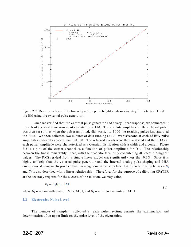
Figure 2.2: Demonstration of the linearity of the pulse height analysis circuitry for detector D1 of the EM using the external pulse generator.

Once we verified that the external pulse generator had a very linear response, we connected it to each of the analog measurement circuits in the EM. The absolute amplitude of the external pulser was then set so that when the pulser amplitude dial was set to 1000 the resulting pulses just saturated the PHA. We then collected two minutes of data running at 100 events/second at each of fifty pulse amplitudes uniformly spaced from 0-1000. The returned events were then analyzed and the PHAs at each pulser amplitude were characterized as a Gaussian distribution with a width and a center. Figure 2.2 is a plot of the center channel as a function of pulser amplitude for D1. The relationship between the two is remarkably linear, with the quadratic term only contributing -0.3% at the highest values. The RMS residual from a simple linear model was significantly less that 0.1%. Since it is highly unlikely that the external pulse generator and the internal analog pulse shaping and PHA circuits would conspire to produce this linear agreement, we conclude that the relationship between and is also described with a linear relationship. Therefore, for the purpose of calibrating CRaTER at the accuracy required for the success of the mission, we may write,

(1) where is a gain with units of MeV/ADU, and is an offset in units of ADU.

2.2 Electronics Noise Level

The number of samples collected at each pulser setting permits the examination and determination of an upper limit on the noise level of the electronics.

32-01207 10 Revision A-

Figure 2.3 is a plot of the width of the Gaussian distributions as a function of the center of each Gaussian for a range of pulse amplitudes. These measurements were taken with the instrument operating in a refrigerator at -40°C. Results are plotted for four of the six detectors. The width of the distribution is clearly a linear function of the amplitude of the pulses, or a fixed fraction of the amplitude. For these measurements the noise is approximately 0.15% of the pulse amplitude, well below the maximum noise level requirement. However, it is important to make two notes. First, this noise measurement does not include the inherent noise of the detectors since the calibration signals are injected after the detectors and therefore do not contribute to these measurements. Second, it is quite likely that the measured noise is a combination of the noise in the pulse shaping and PHA circuitry within the instrument and any noise produced by the external pulse generator itself. These measurements therefore are an upper limit on the true noise level of the CRaTER analog electronics of 1 ADU or 0.02% of the maximum energy.

Figure 2.3: Standard deviation of PHA values returned as a function of center of distribution for ten externally generated pulse amplitudes for four detectors with the telescope operating at -40C. The noise level of the electronics is a constant fraction of the input pulse amplitude, and is less than about 0.15%.

2.3 Stabil ity

While the internal pulse generation system is mainly used for verifying instrument functionality and not for precise calibration purposes, it is useful for tracking the stability of the instrument over time. Each time the EM was transported to the MGH and BNL beam facilities it was common to conduct a full sweep through all of the possible amplitudes of the internal calibration system. Figure 2.4 is a plot of an analysis of the center and width of the response of the D2

32-01207 11 Revision A-

electronics to an amplitude 100 pulse (the internal calibration system has a variable amplitude from 0-255) for four internal calibration runs spaced over four months. The variation in the response over this period, using calibrations taken under very different operating situations and locations, is stable at the 0.06% level.

Figure 2.4: Center of a peak generated by the internal pulse generator from four internal calibration runs spaced over four months showing that the instrument response remained steady at the 0.06% level.

2.4 Temperature Dependence

The temperature dependence of the CRaTER electronics may be determined by placed the instrument in a thermal chamber while feeding pulses through the chamber wall from the external pulse generator, which is maintained at room temperature. Figure 2.5 shows the response of the D2 electronics to a fixed external pulse amplitude as a function of temperature from 24-46C. Over this range the temperature dependence appears to be a linearly decreasing function of temperature, with a slope of -0.21 ADU/C. Over the whole range, this amounts to a shift of -4.7 ADU, or a -0.2% shift from the value at the center temperature.

Figure 2.6 is a plot of the response of D1 to a fixed external amplitude as a function of a broader range of temperatures. In this case the relationship between gain and temperature is seen to be slightly more complex, with a peak at approximately -15C. On the other hand, the total variation is less than 0.1%, as long as the shifted points from a different thermal study at higher temperatures is excluded. We conclude that the thermal dependence of the instrument response is on the order of a 1% level effect, and that a simple linear or bilinear function should be sufficient to describe it. Care should be taken to exercise the FM over the full temperature range with a single experimental configuration so consistent data may be compared.

32-01207 12 Revision A-

Figure 2.5: Response of D2 measurement chain to a constant externally generated pulse as a function of telescope temperature from 23-47C.

Figure 2.6: Response of D1 measurement chain as a function of fixed external pulse generator amplitude for telescope temperatures ranging from -40-45C. Total change is 0.1% and the noise level appears to increase slightly at lower temperatures. The temperature dependence may be described sufficiently with two linear functions and a breakpoint at -15C. The measurements from

32-01207 13 Revision A-

20-45C were taken with a different system and may have produced different values because of different cable lengths, number of cables, or vibration environment.

3 Theoretical Background for CRaTER Calibration This section provides the theoretical basis for our ability to calibrate CRaTER using a spread

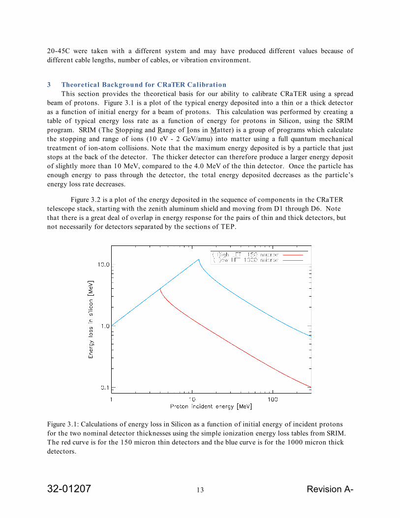
beam of protons. Figure 3.1 is a plot of the typical energy deposited into a thin or a thick detector as a function of initial energy for a beam of protons. This calculation was performed by creating a table of typical energy loss rate as a function of energy for protons in Silicon, using the SRIM program. SRIM (The Stopping and Range of Ions in Matter) is a group of programs which calculate the stopping and range of ions (10 eV - 2 GeV/amu) into matter using a full quantum mechanical treatment of ion-atom collisions. Note that the maximum energy deposited is by a particle that just stops at the back of the detector. The thicker detector can therefore produce a larger energy deposit of slightly more than 10 MeV, compared to the 4.0 MeV of the thin detector. Once the particle has enough energy to pass through the detector, the total energy deposited decreases as the particle’s energy loss rate decreases.

Figure 3.2 is a plot of the energy deposited in the sequence of components in the CRaTER telescope stack, starting with the zenith aluminum shield and moving from D1 through D6. Note that there is a great deal of overlap in energy response for the pairs of thin and thick detectors, but not necessarily for detectors separated by the sections of TEP.

Figure 3.1: Calculations of energy loss in Silicon as a function of initial energy of incident protons for the two nominal detector thicknesses using the simple ionization energy loss tables from SRIM. The red curve is for the 150 micron thin detectors and the blue curve is for the 1000 micron thick detectors.

32-01207 14 Revision A-

Figure 3.2: The same calculation carried out in Figure 3.1, but now for every component within the telescope stack, for protons at normal incidence from deep space, showing the regions of peak energy response for each detector in the telescope.

In reality, the situation is more complex than the relations shown in Figures 3.1 and 3.2. This is because the SRIM code only described the proton energy loss in a statistical sense. It also does not include physics such as nuclear interactions, deep inelastic scattering, and weak interactions such as pion production. Geant4 is a more sophisticated toolkit for the simulation of the passage of particles through matter with an abundant set of physics processes to handle diverse interactions of particles with matter over a wide energy range. For many physics processes a choice of different models is available, and overall the results are much more realistic than the simple SRIM calculations. Figure 3.3 is similar to Figure 3.1, but it has been generated using Geant4.

32-01207 15 Revision A-

Figure 3.3: A scatter plot of the energy deposited in a pair of thin and thick detectors as a function of incident energy. Unlike the previous two calculations shown in this section, this simulation makes use of the Geant4 code, which includes more accurate physics including scattering and nuclear interactions.

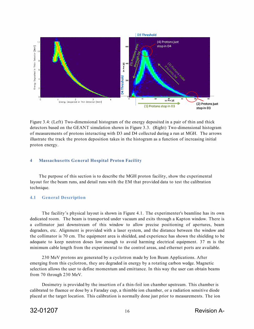
The histogram on the left in figure 3.4 shows the distribution of energy deposits in a think and thick pair of detectors expected by a normally incident beam of protons with a uniform distribution of energy. For this figure, only particles that produced a signal in both detectors were included in the histogram. Additionally, this simulation only went up to 15 MeV, to the track traced by the protons with increasing energy stops at MeV. The plot on the right side of Figure 3.4 is a two dimensional histogram of protons measured by detectors D3 and D4 the EM during a beam run at MGH on May 5, 2007. While the axis of the second plot are in units of ADU instead of MeV, it is clear that the same characteristic track can be seen in the observations. The five key trajectories in the track are labeled: (1) protons stop in D3; (2) protons just stop in D3; (3) protons make it further into D4 with increasing energy; (4) protons just stop in D4; (5) protons pass through D4. Since we have previously shown that the relationship between the and is a simple linear function, the absolute response of each detector in the instrument can be determined by varying the gains and offsets of each detector until the two plots shown in Figure 3.4 coincide.

32-01207 16 Revision A-

Figure 3.4: (Left) Two-dimensional histogram of the energy deposited in a pair of thin and thick detectors based on the GEANT simulation shown in Figure 3.3. (Right) Two-dimensional histogram of measurements of protons interacting with D3 and D4 collected during a run at MGH. The arrows illustrate the track the proton deposition takes in the histogram as a function of increasing initial proton energy.

4 Massachusetts General Hospital Proton Facil ity

The purpose of this section is to describe the MGH proton facility, show the experimental layout for the beam runs, and detail runs with the EM that provided data to test the calibration technique.

4.1 General Description

The facility’s physical layout is shown in Figure 4.1. The experimenter's beamline has its own dedicated room. The beam is transported under vacuum and exits through a Kapton window. There is a collimator just downstream of this window to allow precise positioning of apertures, beam degraders, etc. Alignment is provided with a laser system, and the distance between the window and the collimator is 70 cm. The equipment area is shielded, and experience has shown the shielding to be adequate to keep neutron doses low enough to avoid harming electrical equipment. 37 m is the minimum cable length from the experimental to the control areas, and ethernet ports are available.

230 MeV protons are generated by a cyclotron made by Ion Beam Applications. After emerging from this cyclotron, they are degraded in energy by a rotating carbon wedge. Magnetic selection allows the user to define momentum and emittance. In this way the user can obtain beams from 70 through 230 MeV.

Dosimetry is provided by the insertion of a thin-foil ion chamber upstream. This chamber is calibrated to fluence or dose by a Faraday cup, a thimble ion chamber, or a radiation sensitive diode placed at the target location. This calibration is normally done just prior to measurements. The ion

32-01207 17 Revision A-

chamber is setup to send information about flux and total dosage in real time to monitoring apparatus located in the control room.

The most commonly employed energies are 160 and 230 MeV. 160 allows currents to 15 nA, while 230 allows currents of 80 nA. In all cases these currents can be stopped down with energy degraders. Small diameter beams---less than 1 cm---or targets where uniformity isn't crucial use the unscattered beam spot directly from the cyclotron. Medium diameter beams---from 1 to 5 cm---use a single scatterer to get a Gaussian of the right size and then employ a collimator to produce a central flat region. Medium diameter beams---from 1 to 5 cm---use a double scattering arrangement. The second scatterer is contoured to use incident protons efficiently, and allows beams to 20 cm. All beams make a circular spot, though this can be changes with custom collimators.

The bottom schematic in Figure 4.1 shows the functional layout of the beam tests conducted at MGH. The EM is mounted on a tripod so the telescope is within the beam line. The 1 Hz clock, DC power supply, and 1553 GSE interface are placed behind a wall to shield from the radiation present within the room when the beam is operating. A Linksys router in the office connects the GSE to the wireless network, permitting computers in the office to command the instrument, record returned telemetry to the permanent archive, and display scientific data in real time.

32-01207 18 Revision A-

Figure 4.1: (Top) Architectural drawing of the layout of the proton facility at MGH with the beam dump cave (blue), office (pink), and control center (green) indicated. (Bottom) Schematic diagram indicating the flow of commands and telemetry and the organization of hardware for a beam run.

4.2 CRaTER Setup in Cave at MGH Figures 4.1 through 4.4 illustrate the setup of the CRaTER EM for a test at MGH conducted on

May 5, 2007.

32-01207 19 Revision A-

Figure 4.2: Photograph of the CRaTER EM mounted in the MGH beam line.

Figure 4.3: The CRaTER EM mounted in the MGH beam line as viewed from the side.

32-01207 20 Revision A-

Figure 4.4: Alignment of the CRaTER instrument with the beam is checked by playing a partially reflecting plastic film against the metal face of the CRaTER support brace. This face of the brace is parallel to the instrument telescope symmetry axis. The orientation of the telescope is adjusted until the laser is observed to reflect back down the beam line.

4.3 CRaTER EM Measurements at MGH The data used to test the CRaTER calibration technique were taken on the afternoon of May

05, 2007 with the EM. The plots analysis described in the following section makes use of the beam run archived in the file CRA1020070505155539L0. For this run, the proton beam was set at its maximum energy of 230 MeV. A large quantity of material was then placed in the beam to degrade the protons down to below 33.5 MeV with a very large spread in energy.

Figure 4.5 is a plot of the D1 singles rate as a function of time for this run. As is often the case at MGH, especially when running at low rates, the rate slowly changed over the course of the integration. In total, 460,000 events were analyzed and sent through the GSE for archiving. Figure 4.6 is a 2D histogram of the energy deposits in D1 and D2 collected during the run. The color scale represents the logarithm of the number of events in each bin.

32-01207 21 Revision A-

Figure 4.5: A plot of the D1 event rate as a function of elapsed seconds from the start of run saved in file CRA1020070505155539L0.

32-01207 22 Revision A-

Figure 4.6: Two-dimensional histogram of real measurements of particles interacting with D1 and D2 in a beam run with the CRaTER EM at MGH. Only events producing a detectible signal in both detectors are shown.

5 Calibration This section is divided into two parts. In Section 5.1 a theoretical description of the calibration

process is provided. In Section 5.2 the D1 D2 data described in Section 4.3 are used as a test case to verify the calibration method.

5.1 Theoretical Description

Figure 5.1: (Left) histograms showing the range of initial proton energies selected from a GEANT numerical simulation on the. (Right) For each histogram on the left, the corresponding distribution of energies deposited in the thin and thick detectors.

Our expectation from the MGH beam operator is that the degraded proton beam has a very large spread in energy. While the spread is broad, it is not uniform, and an analysis of the distribution of events shown in the histogram in Figure 4.6 suggested that the distribution appeared Gaussian with a peak energy above the range of both detectors. This is consistent with our notes, which record an expected peak energy of 34 MeV, whereas the peak in D2 (nearing the high side of the energies we are interested in) occurs at 12 MeV. The location of the peak is illustrated graphically in Figure 5.1,

32-01207 23 Revision A-

which shows predicted 2D histograms of D1 D2 energy deposition for two 2 MeV ranges of initial proton energy. For the following calculations we will assume that the incident proton beam has a Gaussian energy distribution with width , center energy , and total flux .

Figure 5.2: A flow chart illustrating the calibration process. A simulated PHA 2D histogram is generated by using the best guess calibration free parameters to convert simulated deposited energies into ADC channels. A full simulated response is created by generating synthetic histograms over a range of incident energies and then integrating over the histograms with weighting determined by the best guess for the beam center energy and width. The simulation is compared with the observations and the free parameters are adjusted until the model converges with the observations.

The calibration process is illustrated as a flow chart in Figure 5.2. We begin by selecting all of the beam data that produced a signal in both of the detectors for a given detector pair. A 2D histogram is then generated, with histogram intervals varied appropriately to achieve good resolution of the proton trajectory traced out in the histogram. An initial guess is then made for the beam parameters, described in the previous paragraph, along with the free parameters of the instrument response model. The parameters for the two detectors, using D1 and D2 as the example, are

, where the are the gains, the are the offsets, and the are a figure representing the scatter of the incoming particles. Early testing of this technique has shown that the Geant4 simulations produce tracks in the 2D histogram which are too narrow. Adding a small Gaussian random fractional scattering term to the individual deposited energies from the simulations improved the agreement between the observations and the best fit model by more than a factor of two. These scattering terms are a combination of the detector noise and the fact that the protons actually arrive in the telescope over a small range of angles of incidence. A more sophisticated simulation should be produced that includes a realistic amount of scatter in angle given the geometry of the setup in the beamline and the expected angular dispersion of the protons emerging from the beam.

32-01207 24 Revision A-

Once an initial guess for the model parameters has been set, the algorithm proceeds as shown in the flow chart. The calibration is used to convert deposited energy into ADUs. The initial incident energy is then sub divided into a number of intervals. For each interval in initial energy, a 2D histogram of simulated measurements is generated. Once this has been done for all energies, the total simulated response is determined by integrating over incident energy, with a weighting by energy given by the current guess for the distribution of the incident proton beam. The resulting prediction is then compared with the observations. If they are in agreement, the values are reported. Otherwise new guesses are made and the process iterates once it has converged on the best fit solution.

5.2 Application of Calibration to the EM

This section illustrates the calibration process described in the previous section for the D1 D2 pair of detectors and the May 5, 2007 data collected at MGH described in Section 4.3. Standard χ2/ν techniques have not yet been successful at identifying the best fit of the model with the measurements. This is for two reasons. First, the predicted response is a very strong and non-linear function of the instrument calibration parameters. This is good because it means this calibration is very sensitive and will place strong constraints on the ADU to energy conversion, but it does mean the initial guess has to be very close to the final value for classical fitting techniques to succeed. The other problem, which can be seen in the following plots, is that the 250,000 simulated particles used for this analysis, and the 460,000 events collected by the EM at MGH, weren’t quite enough to get develop good statistics on the histograms. It appears that this is more a matter of the simulated particles, and for the FM a larger simulation will be conducted.

The algorithm described in the previous section was implemented using an iterative process. First, a conservative possible range for each parameter was identified by eye. A program then stepped through each parameter, evaluating the simulated response for 100 values spaced between the limits. The value of the parameter that produced the minimum χ2/ν was selected as the new value, and the process moved on to the next parameter. After all free parameters were stepped through, the process begins again, but the range of values explored for each parameter is centered around the new value and the width of the range is reduced by 10%. This loop was iterated several dozen times, resulting in an overall reduction of χ2/ν by several hundred from the initial guess to a final value of χ2/1092 = 1.90. One step in this process is shown in Figure 5.3.

Two representations of the final results are shown in Figures 5.4 and 5.5. The first is the same 2D histogram that was shown in Figure 4.6, but with over plotted contours indicating the best fit simulation. The second, Figure 5.5, is a scatter plot of the observed and predicted values, with error bars and a red line indicating parity. A table at the end of this section lists the final derived values.

32-01207 25 Revision A-

Figure 5.3: Plots of the reduced χ2/ν as each of the free parameters in the model are varied by a small amount while the others are held fixed. This series of plots was generated at the first step of an iterative process which ultimately fit the observations with χ2/ν ~ 1.8.

32-01207 26 Revision A-

Figure 5.4: The color background is a 2D histogram of the logarithm of the number of measurements of energy deposits in D1 and D2. The diamonds indicate the points in the histogram that were selected for the fitting process. The black lines are the best fit model prediction.

32-01207 27 Revision A-

Figure 5.5: Scatter plot of the measured and predicted values for the selected points shown in Figure 5.4.

Parameter Value Units D1 Gain 0.0768051 MeV/ADU D1 Offset 1.62984 ADU D2 Gain 0.0249125 MeV/ADU D2 Offset -4.22239 ADU Beam Peak 19.2745 MeV Beam Width 25.2324 MeV Intensity 0.118187 106 protons D1 Noise 1.58370 % D2 Noise 4.80770 %

6 Flight Model Calibration Plan The calibration plan for the FM is described in this section and is divided into three parts.

6.1 Linearity and Noise Following the technique described in Section, the linearity and the electronic noise level of the

FM will be determined using the external pulse generator.

• Connect one of the detector analog measurement circuits to the external pulse generator using the interface port on the side of the telescope

• Set the maximum amplitude of the pulse generator so it just saturates the PHA • Apply fifty pulse amplitudes spaced uniformly across the range of the PHA, with a

minimum of 2 minutes integration at each amplitude, recording the applied amplitude for each integration

• Repeat for the other five detectors • Determine the mean and standard deviation of the PHA ADC values for each setting of

the external pulse generator • Characterize the linearity of each measurement chain by determining the coefficients

for a linear fit and a quadratic fit to the relationship between pulser amplitude setting and average ADU of the PHA. Also record the RMS deviation of the results from the linear curve

• Characterize the width of the distributions as a function of amplitude

6.2 Temperature Dependence The telescope will be placed in a thermally controllable chamber with the ability to cycle the

instrument over the full operating range. Six cables will run from the six ports on the feed through at the telescope out from the chamber.

• Step through eight temperatures that span the operating range • At each temperature hook each circuit up to the external pulse generator and

accumulate for 2 minutes at ten different values of pulse amplitude • Fit a line to the data at each temperature, determine how gain and offset change as a

function of temperature • Look at an individual pulse amplitude as a function of temperature and make sure the

results are consistent with the previous step.

32-01207 28 Revision A-

• IF NEEDED: Cool instrument off, slowly allow to heat to room temperature while recording response to a fixed amplitude pulse

6.3 Beam • Align the telescope with the beam line, zenith side facing the beam. • Set the beam to its maximum energy • Set the discriminator mask to require D5 and D6 to trigger • Degrade the beam until it is spread between D5 and D6, using the D5 histogram to

verify that the beam energy has a good spread in the two detectors • Collect one million particles at ~ 1,500 events / second rate – 20 minutes • Repeat the last three steps for D3 and D4, and then D1 and D2, resetting the mask as

needed • Shut off the beam and reverse the telescope • Repeat the previous three beam runs in the reverse order • Simulate one million particles with a uniform energy distribution covering the range of

each detector pair • Run the analysis described in the previous section to determine the absolute calibration