crash, boom, bang! - gtc on-demand featured...
TRANSCRIPT

CRASH, BOOM, BANG! LEVERAGING GAME PHYSICS AND GRAPHICS APIS FOR SCIENTIFIC
COMPUTING
Peter Messmer, NVIDIA

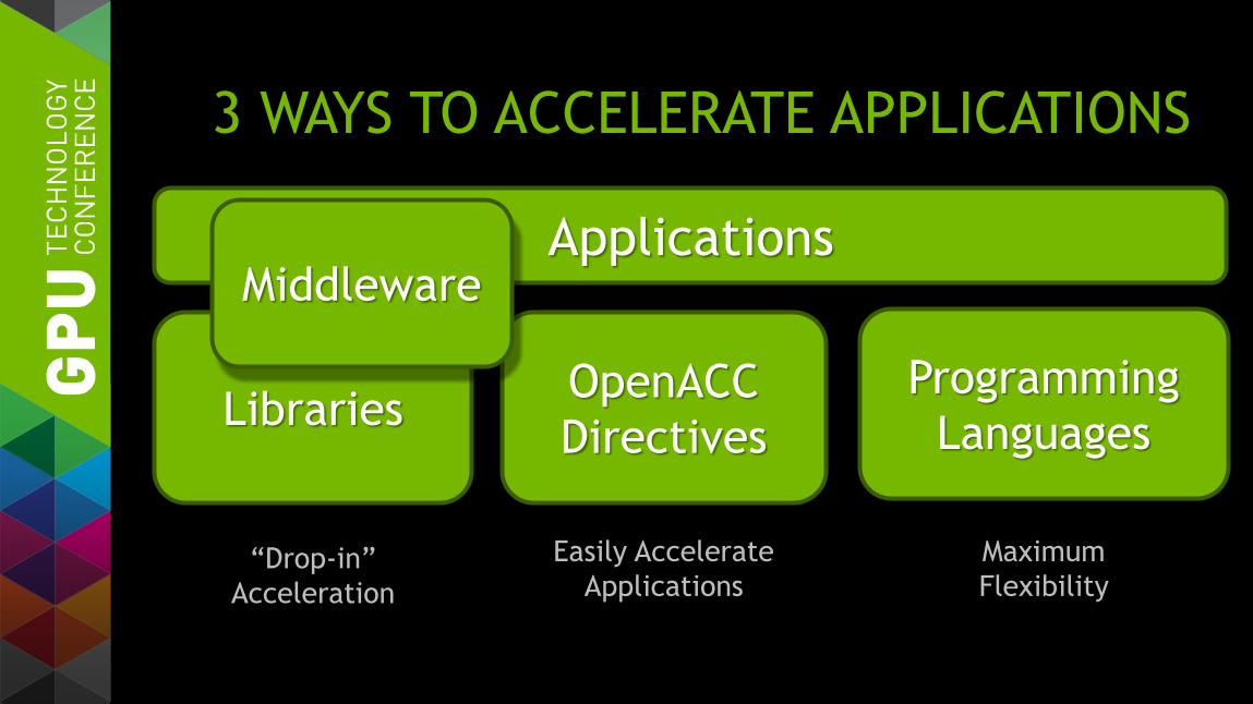
3 WAYS TO ACCELERATE APPLICATIONS
Applications
Libraries
“Drop-in”
Acceleration
Programming
Languages OpenACC
Directives
Maximum
Flexibility
Easily Accelerate
Applications
3 WAYS TO ACCELERATE APPLICATIONS
Applications
Libraries
“Drop-in”
Acceleration
Programming
Languages OpenACC
Directives
Maximum
Flexibility
Easily Accelerate
Applications
Middleware

MOTIVATION
• Similar algorithms in HPC and Entertainment/Media
• Large ecosystem of software developed for E/M Market
What about leveraging E/M software for HPC applications?

MOTIVATION/OUTLINE
• Similar algorithms in HPC and Entertainment/Media
• Large ecosystem of software developed for E/M Market
What about leveraging E/M software for HPC applications?
Step 1: Understand what’s going on in E/M
e.g. PhysX, OptiX
PhysX
PHYSX
A treasure chest, not only for games
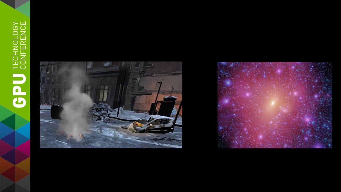

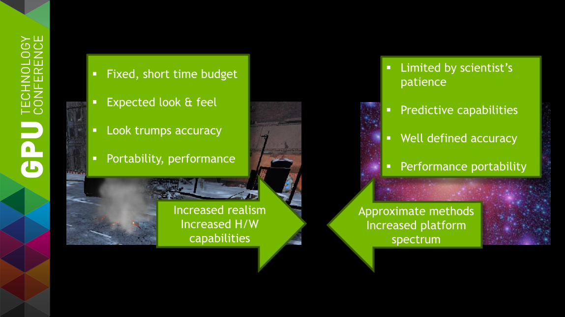
Fixed, short time budget
Expected look & feel
Look trumps accuracy
Portability, performance
Limited by scientist’s
patience
Predictive capabilities
Well defined accuracy
Performance portability
Fixed, short time budget
Expected look & feel
Look trumps accuracy
Portability, performance
Limited by scientist’s
patience
Predictive capabilities
Well defined accuracy
Performance portability
Increased realism
Increased H/W
capabilities
Approximate methods
Increased platform
spectrum

Fixed, short time budget
Expected look & feel
Look trumps accuracy
Portability, performance
Limited by scientist’s
patience
Predictive capabilities
Well defined accuracy
Performance portability
Increased realism
Increased H/W
capabilities
Approximate methods
Increased platform
spectrum
Interactive
Science
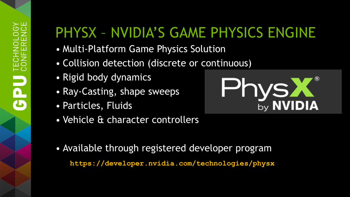
PHYSX – NVIDIA’S GAME PHYSICS ENGINE • Multi-Platform Game Physics Solution
• Collision detection (discrete or continuous)
• Rigid body dynamics
• Ray-Casting, shape sweeps
• Particles, Fluids
• Vehicle & character controllers
• Available through registered developer program
https://developer.nvidia.com/technologies/physx

PHYSX – SOME COOL FEATURES
Rigid Body Dynamics
Particles
Scene queries
Cloth
Vehicles, characters
…
PHYSX – SOME COOL FEATURES
Rigid Body Dynamics
Particles
Scene queries
Cloth
Vehicles, characters
…
Dynamics of shaped
objects with collisions,
constraints
Point particles in
complex environment
Inspection of complex
geometries
Constrained 1D
particle systems
Complex objects with
internal specifications
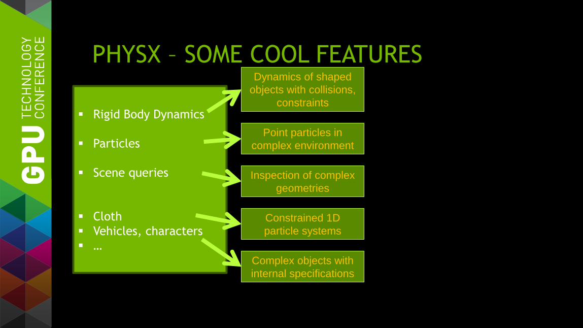
Discrete Element
Method, agent based
simulations
Monte Carlo Methods,
particle methods
Particle-mesh
interaction, CAD-mesh
interactions

RIGID BODY DYNAMICS COMPONENTS
• Collision detection
• Broad Phase => Form potential collision pairs
• Narrow Phase => Identify contact points
• Constraint resolution
• Compute impulses to resolve contacts
• Compute impulses to satisfy constraints
• contacts, joints, friction, ..

CONSTRAINT RESOLUTION
• Linear Complementarity Problem
• Impulses cannot be negative
• Solve for a single body pair
• Multiple constraint resolution
• Iterate over all constraint pairs

A BASIC PHYSX SIMULATION PxFoundation f = PxCreateFoundation(PX_PHYSICS_VERSION,..);
PxPhysics p = PxCreatePhysics(.., *f, .. );
PxScene s = p->createScene(..);
Create PhysX
Attach a Scene
Attach Actors
Simulate Scene
Shutdown
Foundation
Physics
Scene
RigidActor
Shape
BoxGeometry
MeshGeometry
CapsuleGeometry
Material
Density
Friction Coeff

A BASIC PHYSX SIMULATION
• Create two rigid bodies
PxRigidDynamic* body1 = PxCreateDynamic(p,.., g, m,.);
PxRigidDynamic* body2 = PxCreateDynamic(p,.., g, m,.);
• Add bodies to scene
s ->addActor(body1);
s ->addActor(body2);
• Create joint between bodies
PxJoint* joint = PxDistanceCreateJoint(p, body1, .., body2,..)

SUMMARY • Wealth of algorithms relevant to HPC applications
• Possible uses: discrete element simulations, kinetic simulation, optimization problems, ..
• Portable performance
• Core algorithms GPU accelerated
• Free (see license for details)

OptiX
OPTIX
Pretty pictures and more

IF YOUR APPLICATION LOOKS LIKE THIS..

.. YOU MIGHT BE INTERESTED IN OPTIX
• Ray-tracing framework
• Build your own RT application
• Generic Ray-Geometry interaction
• Rays with arbitrary payloads
• Multi-GPU-support

60GHZ ELECTROMAGNETIC PROPAGATION

COLLISION DETECTION / PATH PLANNING

PARTICLE TRACKING WITH OPTIX
• GPU accelerated particle-geometry interaction
• Ultimate use: Simulation of spacecraft engines
• Particle-geometry interaction, change in species, complex dynamics
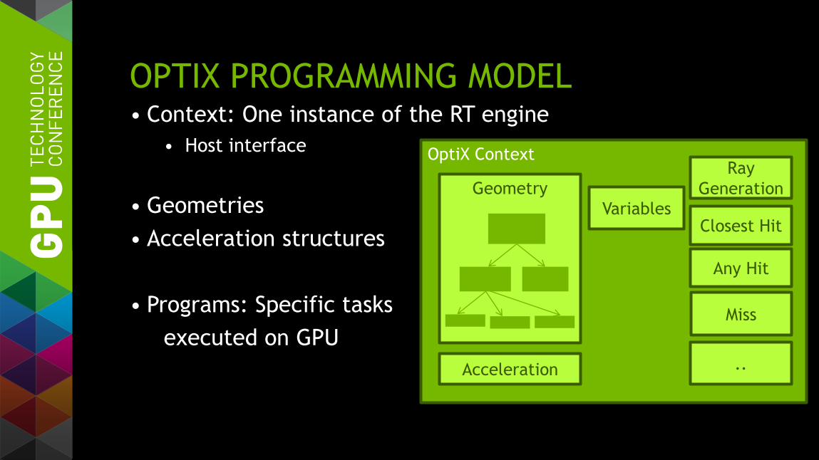
OPTIX PROGRAMMING MODEL • Context: One instance of the RT engine
• Host interface
• Geometries
• Acceleration structures
• Programs: Specific tasks
executed on GPU
OptiX Context Ray
Generation
Closest Hit
Any Hit
Miss
..
Geometry
Acceleration
Variables
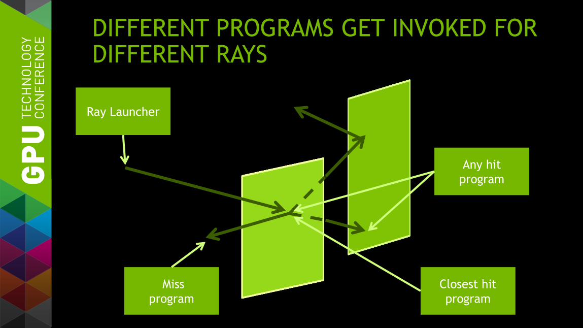
DIFFERENT PROGRAMS GET INVOKED FOR DIFFERENT RAYS
Ray Launcher
Closest hit
program
Any hit
program
Miss
program

HOW DO OPTIX PROGRAMS LOOK LIKE? struct PerRayData_radiance
{
float3 result;
};
rtDeclareVariable(PerRayData_radiance, prd_radiance, rtPayload, );
rtDeclareVariable(float3, bg_color, , );
RT_PROGRAM void miss()
{
prd_radiance.result = bg_color;
}
Ray’s payload
Define the ray’s
payload
The miss program

HOW DO OPTIX PROGRAMS LOOK LIKE? struct PerRayData_radiance
{
float3 result;
};
rtDeclareVariable(PerRayData_radiance, prd_radiance, rtPayload, );
rtDeclareVariable(float3, bg_color, , );
RT_PROGRAM void miss()
{
prd_radiance.result = bg_color;
}
Ray’s payload
Define the ray’s
payload with semantic
variable
The miss program

RAY LAUNCHER: PROGRAM EXECUTED FOR EACH RAY RT_PROGRAM void pinhole_camera()
{
size_t2 screen = output_buffer.size();
float2 d = make_float2(rtLaunchIndex) / make_float2(screen) * 2.f - 1.f; float3 ray_origin = eye;
float3 ray_direction = normalize(d.x*U + d.y*V + W);
optix::Ray ray(ray_origin, ray_direction, radiance_ray_type, scene_eps);
PerRayData_radiance prd;
prd.importance = 1.f;
prd.depth = 0;
rtTrace(top_object, ray, prd);
output_buffer[rtLaunchIndex] = make_color( prd.result ); }
Determine per ray
direction
Create the ray
Launch the ray
Store result into
result buffer
Not limited to planar launcher!

GEOMETRY • Tree structure of geometry instances
• Association geometry-programs
• Different programs for different parts of the geometry possible
• Acceleration structures
• Enable quick scene queries
• Requires BoundingBox program
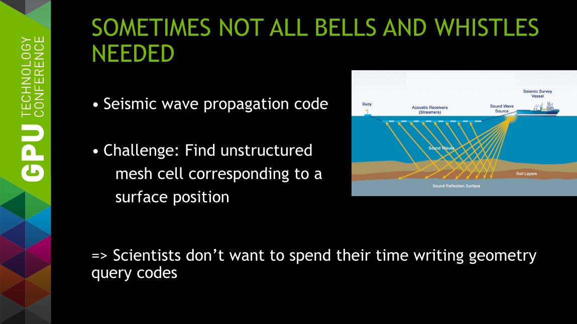
SOMETIMES NOT ALL BELLS AND WHISTLES NEEDED
• Seismic wave propagation code
• Challenge: Find unstructured
mesh cell corresponding to a
surface position
=> Scientists don’t want to spend their time writing geometry query codes

OPTIX PRIME: LOW-LEVEL RAY TRACING API
•OptiX simplifies implementation of RT apps • Manages memory, data transfers etc
•Sometimes all you need are visibilities • E.g. just need visibility of triangulated geometries
•OptiX Prime: Low-Level Tracing API
• User provides geometry, rays, OptiX returns hits
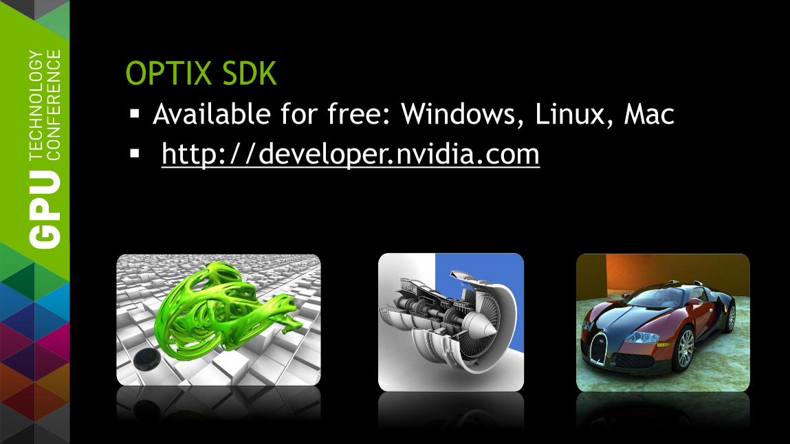
OPTIX SDK
Available for free: Windows, Linux, Mac
http://developer.nvidia.com
SUMMARY
Overlap of algorithms used in E/M and HPC
PhysX
— Examples: Rigid body dynamics, particles
OptiX
— GPU accelerated ray-tracing
— OptiX Prime for basic ray-geometry intersection tests

ABSTRACT (FOR REFERENCE ONLY) In this talk, you will learn how to use the game and visualization wizard's tool chest to accelerate your scientific computing applications. NVIDIA's game physics engine PhysX and the ray tracing framework OptiX offer a wealth of functionality often needed in scientific computing application. However, due to the different target audiences, these frameworks are generally not very well known to the scientific computing communities. High-frequency electromagnetic simulations, particle simulations in complex geometries, or discrete element simulations are all examples of applications that could immediately benefit from these frameworks. Based on examples, we will talk about the basic concepts of these frameworks, introduce their strengths and their approximation, and how to take advantage of them from within a scientific application.