AFFDL-TR-74-129 Fi fio•c cA-' c•_E -\-

Volume I

19bA OX~I 7600

CRACK GROWTH ANALYSIS FORARBITRARY SPECTRUM LOADINGVolume I - Results and Discussion

GRUMMAN AEROSPACE CORPORATION

BETHPAGE, NEW YORK

DEL WEST ASSOCIATES, INC.

WOODLAND HILLS, CALIFORNIA

OCTOBER 1974

FINAL REPORT: JUNE 1972 - OCTOBER 1974

TECHNICAL REPORT AFFDL-TR-74-129

Volume I

Approved for public release; distribution unlimited

AIR FORCE FLIGHT DYNAMICS LABORATORY Best Available CopyAir Force Systems CommandWright-Patterson Air Force Base, Ohio 45433

_ oo60 9 t/0Iw/5

NOTICE

When Government drawings, specifications, or other data are used for any purpose

other than in connection with a definitely related Government procurement operation,

the United States Government thereby incurs no responsibility nor any obligation

whatsoever; and the fact that the Government may have formulated, furnished, or in

any way supplied the said drawings, specifications, or other data, is not to be re-

garded by implication or otherwise as in any manner licensing the holder or any other

person or corporation, or conveying any rights or permission to manufacture, use, or

sell any patented invention that may in any way be related thereto.

ROBERT M. BADER, ChiefProject Engineer Structural Integrity BranchFatigue, Fracture & Reliability Gp Structures Division

FOR T COMMANDER

GERALD G. LEIGH, Lt Col, USAFChief, Structures Division

This report has been reviewed by the Information Office (01)and is releasable to the National Technical InformationService (NTIS). At NTIS it will be available to the generalpublic, including foreign nations.

Copies of this report should not be returned unless return is required by security

considerations, contractual obligations, or notice on a specific document.AIR FORCI - 5-2-76 - 500

UNCLASSIFIEDSECURITY CLASSIFICATION OF THIS PAGE (When Data Entered)

REPORT DOCUMENTATION PAGE READ INSTRUCTIONSBEFORE COMPLETING FORM

1. REPORT NUMBER 2. GOVT ACCESSION NO. 3. RECIPIENT'S CATALOG NUMBER

AFFDL-TR-74-129I

4. TITLE (and Subtitle) 5. TYPE OF REPORT & PERIOD COVERED

CRACK GROWTH ANALYSIS FOR ARBITRARY FINAL TECHNICAL REPORT

SPECTRUM LOADING JUNE 1972- OCTOBER 1974

VOLUME I - RESULTS AND DISCUSSION 6. PERFORMING ORG. REPORT NUMBER

7. AUTHOR(a) e. CONTRACT OR GRANT NUMBER(s)

P.D. BELL, M. CREAGER F33615-72-C-1744

9. PERFORMING ORGANIZATION NAME AND ADDRESS 10. PROGRAM ELEMENT, PROJECT, TASK

AREA & WORK UNIT NUMBERS

GRUMMAN AEROSPACE CORPORATIONBETHPAGE, NEW YORK 11714

II. CONTROLLING OFFICE NAME AND ADDRESS 12. REPORT DATE

AIR FORCE FLIGHT DYNAMICS LABORATORY OCTOBER 1974

WRIGHT-PATTERSON AIR FORCE BASE 13. NUMBER OF PAGES

DAYTON, OHIO 45433

14. MONITORING AGENCY NAME & ADDRESS(if different from Controlling Office) I5. SECURITY CLASS. (of this report)

UNCLASSIFIEDSAME

15a, DECLASSI FICATION/DOWNGRADING

SCHEDULE

16. DISTRIBUTION STATEMENT (of this Report)

APPROVED FOR PUBLIC RELEASE; DISTRIBUTION UNLIMITED

17. DISTRIBUTION STATEMENT (of the abstract entered in Block 20, if different from Report)

18. SUPPLEMENTARY NOTES

19. KEY WORDS (Continue on reverse side if necessary and Identify by block number)

CRACK CLOSURE SPECTRUM LOADSCRACK GROWTH INTERACTION 2219-T851 ALUMINUMMATHEMATICAL MODEL Ti 6AI-4V TITANIUM

OVER LOADS

20. ABSTRACT (Continue on reverse aide If necessary and Identify by block number)

THIS COMBINED ANALYTICAL AND EXPERIMENTAL STUDY WAS UNDERTAKEN TO INVESTIGATEFATIGUE CRACK GROWTH INTERACTION EFFECTS AND TO EITHER MODIFY EXISTING CRACKGROWTH RETARDATION MODELS OR TO DEVELOP NEW MODELS. A TEST PROGRAM WAS CONDUCTEDON 2219-T851 ALUMINUM AND ON Ti 6AI-4V TITANIUM CENTER CRACKED PANEL AND COMPACTTENSION SPECIMENS. A VARIETY OF LOADING CONDITIONS, INCLUDING CONSTANT AMPLITUDE,SINGLE AND MULTIPLE OVERLOADS, SINGLE AND MULTIPLE PERIODIC OVERLOADS, SIMPLIFIED

(CONTINUED ON NEXT PAGE)

DD I JRAN7, 1473 EDITION OF I NOV 65 IS OBSOLETE

SECRIT CLA UNCLASSI FI EDSECURITY CLASSIFICATION OF THIS PAGE (When Data Entered)

UNCLASSIFIEDSECURITY CLASSIFICATION OF THIS PAGE(Whh, Data Entered)

BLOCK PROGRAMS, COMPRESSION, TENSION-COMPRESSION AND COMPRESSION-TENSION SEQUENCES,WAS INVESTIGATED. LOADING VARIABLES INCLUDED THE RELATIVE MAGNITUDES OF OVERLOADS

AND BASELINE LOADS, FREQUENCY OF OCCURRENCE OF SINGLE AND MULTIPLE PERIODICOVERLOADS, RELATIVE MAGNITUDE OF COMPRESSION SPIKE LOADS AND STRESS RATIO. SIMPLI-FIED BLOCK PROGRAM LOAD VARIABLES INCLUDED ORGANIZING THE LOAD LAYERS AS LOW-

TO-HIGH, HIGH-TO-LOW OR RANDOMIZED LOADS, AND THE INTRODUCTION OF EITHER A SINGLEOVERLOAD CYCLE TO EACH BLOCK OR AN OCCASSIONAL UNDERLOAD. TWO MULTI-LAYERFIGHTER SPECTRUM TESTS WERE INCLUDED. IT WAS CONCLUDED THAT THE CRACK CLOSURE

CONCEPT COULD BE USED TO EXPLAIN A VARIETY OF CRACK GROWTH INTERACTION EFFECTS.AN EMPIRICAL MATHEMATICAL MODEL USING THIS CONCEPT WAS DEVELOPED AND SHOWN TOYIELD REASONABLY ACCURATE PREDICTIONS OF CRACK GROWTH BEHAVIOR FOR MANYLOADING SEQUENCES. THIS MODEL WAS INTEGRATED INTO THE CRACKS II DIGITAL COMPUTERPROGRAM.

UNCLASSIFIEDSECU IlTy CLASSIFICATION OF THIS PAGE(When Date Entered)

FOREWORD -

This report describes an investigation of fatigue crack growth inter-action effects in airframe structural materials performed by the GrummanAerospace Corporation from June 2, 1972 through October 2, 1974 under AirForce Contract F33615-72-C-17 4 4. A portion of the analytical and experimentaleffort was subcontracted to Del Research Corporation and to Del West Associ-ates, Inc.

The work was sponsored under Project 486u, "The Advanced MetallicStructures - Advanced Development Program" (AMS-ADP), Task 486U02, "AppliedFracture Mechanics" Air Force Flight Dynamics Laboratory (AFFDL) withMr. Robert M. Engle (AFFDL/FBE) as project engineer.

The program was conducted by structural mechanics personnel of theGrumman Aerospace Corporation under the supervision of F. Berger, Manager,Advanced Development Systems Engineering. The Project Engineer was A. Wolfman.The principal investigator was P. D. Bell and program test engineering andcoordination was provided by S. Hoops. Technical and experimental supportwas provided by Drs. P. Paris and R. Bucci and program support was providedby D. Schmidt of Del Research Associates. Dr. M. Creager provided technicaland experimental support and W. Renslen provided program support for Del WestAssociates, Inc.

This report was submitted by the authors on October 1, 1974.

A second volume, containing all raw data generated under this program,is available upon request. Send requests to:

AFFDL/FBEAttn: R. M. EngleWright-Patterson AFB, OH 45433

iii

CONTENTS

•Page

SUMMARY . . . . . . . . . . . . . . . . . . . . . . . . . . . . . . . . xiii

1. INTRODUCTION ................... ............................ 1

2. MATERIALS AND PROCEDURES ................... ...................... 32.1 Material Selection ... ...... ..... .......... ............ 32.2 Testing Procedures ..................... ............... ..... 32.3 Specimen Geometry ...................... ....................... 42.4 Crack Closure Measurements ................. ................... 5

3. RESULTS AND DISCUSSION OF TEST DATA •..... . .......... .......... 103.1 Constant Amplitude Test Results .............. ................ 10

3.1.1 Aluminum ............... .......................... . 113.1.2 Titanium ............... ......................... .. 12

3.2 Single Overload Test Results ......... ....................... 143.2.1 Aluminum ............... ......................... .. 153.2.2 Titanium. ................ ........................ .. 263.2.3 Interactions of Overloads ...... ................. .. 28

3.3 Multiple Overload Test Results . . . I............... 293.3.1 Aluminum . ................ ....................... .. 293.3.2 Titanium ............... ......................... .. 32

3.4 Variable Amplitude Test Results ................................. 343.5 Effects of Underloads and Compression Spikes ............. .. 353.6 Miscellaneous Test Results ........... .................. .. 39

3.6.1 Stable Tear .............. ....................... .. 393.6.2 Thickness Effects ..... ........ ........... .... 413.6.3 Tensile Tests .............. ...................... 42

3.7 Summary of Test Results ............ .................... 43

4. MATHEMATICAL MODELING .............. ....................... .. 454.1 Crack Closure Model .. .......... ... ............ .. 46

4.1.1 Concepts ..... ... ............... .... ...... .... 464.1.2 Application to Model ......... ................... .. 504.1.3 Results and Discussion ......... .................. .. 704.1.4 Logic Diagram .............. ...................... 794.1.5 Basic Data Requirements .............. ................. 80

4.2 Residual Force Model ............. ...................... .. 834.1.1 Concepts .... ................ .................. 834.1.2 Application to Model ......... ................... .. 834.1.3 Results and Discussion ......... .................. .. 88

5. SUGGESTIONS FOR FUTURE EFFORTS ......... ................... .. 94

6. OBSERVATIONS AND CONCLUSIONS ........... .................... .. 96

7. REFERENCES ................... ............................. .. 98

V

CONTENTS (Cont)

Page

FIGURES FOR MAIN TEXT ..................... ........................ 100

TABLES FOR MAIN TEXT .................... ........................ 247

APPENDIX A - EQUATIONS ................ ....................... .. 262

APPENDIX B - COMPUTER PROGRAM ............. .................... .. 265

FIGURES FOR APPENDIX B ................ ....................... .. 269

TABLES FOR APPENDIX B ................. ........................ .. 270

APPENDIX C - STRESS INTENSITY FACTOR FOR CTB SPECIMEN ... ........ .. 278

FIGURE FOR APPENDIX C ................. ........................ .. 279

vi

LIST OF SYMBOLS

a - Crack length for compact tension specimens; half-crack lengthfor center cracked panel specimens (inch)'

a - Crack length at which an overload(s) was applied (inch)0

a - Crack length which defines the extent of the material elastic-plastic interface.

a - Difference between crack length and reversed plastic zone radius,a-r (inch)Y

a - Crack length at start of current cyclic loading (inch)s

at - Incremental crack front tunneling (inch)

Aa - Crack growth increment (inch)

Aa* - Crack length over which transient crack growth conditions exist(inch)

B - Empirical exponent in decreasing closure equation, alsodesignation for one block (cyclic loads within one block arerepeated)

b - Dimension along crack (inch)

C - Empirical crackgrowth coefficient

C' - Empirical crack growth coefficient

Cf - Crack closure factor, ratio of K to K (or K), or S to S(or S), or P to P max (or P)

Cf' - Modified crack closure factor

Cf - Crack closure factor at R = zero

0

C - Empirical parameter used in Wheeler retardation modelP

vii

CCP - Center cracked panel specimen

CTA - Compact tension specimen, ASTM geometric proportions =

CTB - Compact tension specimen, modified geometric proportions

COD - Crack opening displacement (inch)

CC 2 - Constants for crack closure instrumentation

c - Surface crack half-length, dimension along crack (inch)

d - Dimension from crack tip to closure gage (inch)

da- Crack growth rate (inch/cycle)

dad-- - Crack growth per block (inch/block)

f - Normalized crack growth rate, ratio of measured crack growth raten to calculated constant amplitude crack growth rate

K - Stress intensity (ksii/T{-h)

K - Stress intensity calculated using the stress or load at whichcrack closure occurs (ksiV'Thnh)

K - Critical stress intensity (ksi/-nch)cr

K - Maximum stress intensity (ksiVin-ch)max

K - Maximum stress intensity caused by an overload (ksiV'n-ch)maxOL

K .- Minimum stress intensity caused by an ov-erload (ksi/'nc)

minoL

K min - Minimum stress intensity (ksi/Th•h)

K - Residual stress intensity (ksii-n-ch)r

Kst - Stress intensity at which stable tear reaches measurable propor-tions (ksi/i-nch)

viii

AK - Stress intensity range, Kmax - Kmin (ksiVi-nch)

AKb - Stress intensity range for baseline loading (ksiV/IF•)

AKeff - Effective stress intensity range, K - K orK - K (ksi/inch) max cmaXO c

OLAKefft - Effective stress intensity range threshold,

K - K (ksiVIn-ch)max c

AK - Stress intensity range threshold at which the crack growthrate is apparently zero (ksiV'7_-h)

AKth -AKth at R = zero (ksi/ii7•h)0

.m - Empirical exponent used in Wheeler retardation model

N - Cycles of load

n - Empirical crack growth exponent

n? - Modified empirical crack growth exponent

ND - Number of delay cycles

N - Cycle count at which an overload(s) was applied0

NOL - Number of overload cycles

Nsat - Number of overload cycles required to produce stabilized closureand, subsequently, maximize retardation

AN - Cyclic increment

AN - Number of load cycles since load changeS

O/L - Overload ratio, ratio of P to P (or P to P )m or S to S(or SOL toSm ) OL OL max xOL

P - Applied load, also maximum applied baseline load (lb)

P -°Load at which crack closure occurs (lb)c

ix

P - Maximum applied baseline load (lb)max

P min - Minimum applied baseline load (lb)

POL - Overload, maximum applied load (lb)

p - Empirical exponent in crack closure equation

q - Empirical crack growth constant

R - Stress or load ratio, Smin/Smax or Pmin/Pmax

- Stress ratio equal to either the applied stress ratio or the

stress ratio cutoff value, R 0 whichever is lessco'

R - Ratio of closure stress or load after a few overload cycles to

the previous (baseline) closure stress or load

R - Stress ratio cutoff value above which crack growth rates areco not stress ratio dependent

r - Reversed plastic zone radius (inch)

Y

S - Applied stress, also maximum applied baseline stress (ksi)

S - Stress required to extend plastic zone from current crackap length to elastic-plastic interface (ksi)

S - Stress at which crack closure occurs (ksi)c

S' - Modified crack closure stress (ksi)c

S - Maximum applied baseline stress (ksi)max

S - Effective maximum stress (ksi)maxeff

S min - Minimum applied baseline stress (ksi)

S - Effective minimum stress (ksi)mineff

x

SOL - Overload, maximum applied stress (ksi)

S - Subscript p indicates previous stress or load (max, min, c, etc.)P

S - Residual stress (ksi)r

Sred - Reduced stress, Sap - S max, (ksi)

ASeff - Effective stress range, S max - S min or Smax (or S) -SC'eff(ksi) maff mlff mx*

t - Specimen thickness (inch)

U -(l - Cf)/(l - R)

V - Displacement voltage from strain gages (volts)

V1 - Load voltage from load cell (volts)

W - Total width of panel specimens; dimension from load line toextreme fiber for compact tension specimens (inch)

S- Relates residual stress to applied stress, a = S /Sr

- Plastic zone coefficient

y - Ratio of closure stress after a few overload cycles to thestabilized closure stress after many overload cycles

r - Denominator in residual force model equation

S- Prefix, micro (10-6

p - Plastic zone radius (inch)

S- Material yield stress (ksi)

y

xi

SUMMARY

This program is one in a series of research and development programsundertaken by the United States Air Force to develop methods and data neededfor design against fracture in military aircraft. This combined analyticaland experimental program was directed to an investigation of fatigue crack -growth interaction effects under arbitrary spectrum loading conditions.

The test program consisted of approximately 160 specimens almostequally divided between 2219-T851 aluminum and Ti 6A1-4V mill-annealed titan-ium alloys. Compact tension and center-cracked panel specimens were employed.All tests were performed under ambient laboratory conditions. The test pro-gram included constant amplitude, single and multiple overload, compressionspike, tension/compression, compression/tension and simplified block loadingsequences.

The results of the experimental program were used to review existingcrack-growth prediction models and finally to develop a new crack-growthprediction model which was based on the crack closure concept. The resultantcrack closure model predicts the crack growth during more complex loadingsequences than existing models. It considers negative stress ratios, numberof overload effects, and the effects of compression spikes with and withoutor preceding or following a tensile spike or multiple overloads,

xiii

1 - INTRODUCTION -

New facture control and damage tolerance criteria (Reference 1 forexample) are being developed and implemented to reduce the risk of the lossof military aircraft due to the existence of crack-like defects in the air-frame structure. These defects can occur through material processing orfabrication techniques in a typical airframe component. As a result, the -criteria specify that flaws be assumed to exist in critical structural loca-tions and, further, that a component be designed in such a way that its lifeexpectancy meets or exceeds the specified life for the aircraft or inspectioninterval before the flaw grows to critical dimensions. A necessary element -in this concept is an analytical method of determining the sub-critical crackgrowth caused by a typical aircraft load spectrum.

This program was initiated by the United States Air Force to modifyexisting models or develop a new model to provide improved predictivecapability for the growth of cracks subjected to arbitrary load spectra. Anexperimental program was conducted to obtain detailed information regardingthe behavior of cracks subjected to discrete and simplified variable-amplitudeloads. The materials tested were 2219-T851 aluminum and Ti 6A1-4V mill-annealed titanium alloys, both typical aircraft structural materials. Withfew exceptions, all tests were performed on 1/4 in.-thick specimens of threegeometries. The loadings employed ranged from constant amplitude to four-level block spectrum loading, and included compression loads. Crack closuremeasurements using three different techniques were obtained during many tests.Crack growth data were obtained during all tests. The frequency of observationvaried, depending on the type of test conducted.

The analytical portion of the program consisted of two basic parts.The first centered around the reduction and analysis of the crack growth data.Crack closure data were investigated to a lesser extent. The second partconsisted of reviewing existing crack growth prediction models with an eyetoward their improvement, and the development of new models. The final mathe-matical model was based on the crack closure concept.

Preliminary investigations indicated that the crack closure conceptcould be used to explain a variety of crack growth interaction effects, in-cluding retardation and acceleration and the effect of different numbers oftensile overloads or compression loads on subsequent crack growth rates.Therefore, the mathematical modeling effort in this program was directedprincipally toward models which employed variations in crack closure to produceeffective stress ranges. The effective stress ranges were then used to cal-culate modified crack growth rates.

It was further thought that since crack closure is a physical phe-nomenon, insight could be gained through direct measurement of crack closureduring crack growth interaction tests. The testing portion of this programrevealed that it was quite difficult to obtain quantitative values of crackclosure during the transient crack growth caused by load perturbations.However, qualitative trends could be observed. The problems encountered inmeasuring crack closure are described in Sections 2 and 3 of this report.

Even though experimental difficulties were encountered, a model basedon crack closure behavior was developed that was found to predict a variety -of crack growth interaction effects quite well. The development of this modeland some results obtained by its application are described in Section 4 ofthis report.

2

2 - MATERIAL AND PROCEDURES

2.1 MATERIAL SELECTION

The selection of the two alloys for flaw growth characterization was

based on the potential widespread utilization of the results from this program.

The materials selected were 2219-T851 aluminum and Ti 6A1-4V mill-annealedtitanium alloys. The crack growth data for these two materials, and the useof that data in the development of crack growth interaction models, was ex-

pected to afford greater confidence in the utility of the results. That is, a

designer employing either material in a new design would have confidence that -

the crack life predictions obtained from the model would be reliable for thesetwo materials.

Each material was obtained in plate form from one material heat. This

was done to minimize the scatter which might be expected when comparing the

crack growth data from two different material heats. The aluminum plates werenominally 5/8 inch thick while the titanium was nominally 3/4 inch thick.

Since a limited thickness effect investigation was included in the program,

all plates were mill polished from the as-received thickness to the requiredspecimen thickness. In this way, the material homogeneity was maintained andthe polishing process introduced minimal surface residual stresses.

2.2 TESTING PROCEDURES

Fatigue crack growth tests were performed using a variety of closed-

loop servo-hydraulic testing machines. Different machines, which will not be

listed here, were employed for economy in testing the various geometries and

because the testing was performed in three different laboratories. One machine

utilized a computer control, while others employed paper tape control to per-form the two-, three- and four-level block loading tests.

Crack growth measurements were obtained optically from the surface of

the specimens. In many cases, the surface crack lengths were measured on both

sides of the specimen. The optical instruments were matched to the type of

test performed so that low-power instruments were used where gross values ofcrack length increments (>0.030 inch) were required whereas high-powered

instruments were used at the other extreme. These latter instruments provided

the capability of directly reading the crack length to 0.001 inch.

Testing frequency varied according to the machine, material and

specimen geometry. In most cases, the cyclic frequency exceeded 1 Hz. Alltests were performed in a laboratory environment at ambient temperature and

relative humidity. The exception was that one compact tension specimen of

each material was tested under constant amplitude loading conditions in a 95%relative humidity environment at various cyclic frequencies. The results from

3

these tests compared favorably with those from the laboratory air environment

and are reported in Section 3 of this report.

The ambient temperature ranged from 65 to 75 degrees F while the

relative humidity had a considerably larger range. Relative humidity measure-

ments are reported on the data sheets included in Volume II.

Crack closure measurements were performed using two different tech-

niques. The procedures and equipment are reported in Subsection 2.4.

Material tensile properties were obtained from six aluminum tensilespecimens. For two thicknesses (1/4 inch and 3/4 inch), four titanium tensilespecimens each were used to obtain tensile properties for the titanium. Alltensile specimens were oriented in the longitudinal grain direction and wereselected randomly from the plates. The machine employed was a Riehle FH 60Universal Testing machine and the extensometer was a DN-20 with a 2 in. gagelength. The material tensile properties are presented in Subsection 3.5.3.

All specimens were precracked at load levels selected to provide aminimum amount of interaction with the test loads, or fast crack initiation,or at the load level used for the test. All precracking loads are specifiedin Volume II of this report.

2.3 SPECIMEN GEOMETRY

Three different basic specimen geometries were employed for this pro-gram. These were the center cracked panel shown in Figure 1 and the twovarieties of compact tension specimen shown in Figure 2.

The center cracked panel (CCP) specimens were of nominally constantgeometry with a thickness of .25 in. and a width of six inches in the testsection. Crack starter notches were electro-discharge machined into one sur-face of the specimens at the longitudinal and lateral centerlines. Thestarter notches were of constant radius approximately 0.025 inch deep, 0.10inch long on the surface and 0.010 inch wide. Some of the panels were loadedin compression. To prevent column buckling, the panels were enclosed in a

stabilizing fixture which was separated from the specimen by Teflon liners.One specimen was fitted with strain gages to ensure that the stabilizingfixture did not pick up load through friction.

The compact tension specimens were of two geometries. Those testedby the Del organizations were of the standard ASTM geometry except that thethickness relationship specified for plane strain conditions was not retained.These specimens are defined as CTA specimens in Figure 2. Almost all werefabricated with dimension W = 2.5 inches. A few were fabricated withW = 2.2 inches to economize on material so that the material heat would beconstant.

14

The compact tension specimens tested by Grumman were modified from theASTM proportions and are defined as CTB specimens in Figure 2. The basicdifference was that the height of these specimens was increased to provideclearance for the Amsler "Movomatic" displacement gage (described in Sub-section 2.4). The stress intensity solution for the CTB geometry is presentedin Appendix C.

All specimens were oriented with the load line parallel to the rolling(longitudinal grain) direction so that the crack grew normal to the rollingdirection. -

Compact tension specimen identification numbers consist of a pair ofletters and two numerical pairs: (ie. AD-25-32 or TG-25-12). The firstletter designates the material (A=2219-T851 aluminum, T=Ti 6A1-4V titanium)while the second letter indicates the testing laboratory (G=Grumman, D=DelResearch or Del West). The specimens with a D designation were all of ASTMstandard geometry (CTA) while those with a G were non-standard (CTB) or center-cracked panels. The first pair of numbers represents the nominal materialthickness in hundredths of an inch while the second pair is the specimensequence number. A few compact tension specimens had duplicate sequencenumbers, so the lower case letter a was added following the sequence number.

In the case of center-cracked panel specimens, the system is the sameexcept that a P is appended (ie. AG-25-12P).

2.4 CRACK CLOSURE MEASUREMENTS

Preliminary analyses and the work reported by a number of authorsindicated that variations in crack closure might be used to describe a variety.of crack growth interaction effects. Because of this, crack closure measure-ments were obtained during many specimen tests. The objectives were toquantify the crack closure level as a function of stress ratio during steady-state constant-amplitude conditions, and to define how the closure level variedduring transient conditions such as during the application of overloads andwhile the crack was propagating subsequent to the application of one or moreoverloads. Measurements were also obtained during loading sequences in whichthe maximum load was held constant and the minimum load was varied. In a fewcases, the minimum load was allowed to go into compression. Closure measure-ments were also obtained during simplified block-loading sequences.

Although some authors have observed differences in the magnitudes ofthe opening and closure loads, no significant differences were observed duringthis program. As a result, the terms opening and closure are used inter-changably and are considered to be the same value of load or stress.

Two different methods were employed to measure crack closure. Thefirst employed strain gages mounted across the crack tip, while the secondemployed a mechanical displacement gage similarly located. These techniqueswill be described below.

5

The principal conclusion drawn from this investigation was that

meaningful quantitative values of closure could be obtained only during steady-

state conditions. These were either constant-amplitude loading or periodic

block-loading situations. In the case of periodic loading, the closure levelgenerally did not vary significantly within a block of loads and, as such,approached steady-state conditions. Even for steady-state conditions, how-ever, significant amounts of scatter were encountered. Generally, for a

given specimen and gage location, the results were repeatable. However, ifthe gage was moved or if a different gage were employed, repeatabilitydeteriorated. The final conclusion drawn from these results was that quanti-tative closure measurements, useful for modeling purposes, could not be ob-tained using the methods described below. However, the data obtained did

prove useful from a qualitative standpoint and provided justification formany of the assumptions made during the modeling effort.

Crack closure measurements made at Del Research and at Del Westutilized a technique developed by R. Schmidt (Ref 2) to measure crack closure.The objective of the closure measurement was to monitor the relationshipbetween applied loads and the local crack displacements, and to note the load

level in this relationship where it becomes non-linear (See Figure 3).Schmidt utilized an electrical resistance strain gage bonded to the specimen

at its ends only to measure local displacements, as shown in Figure 4, ratherthan a mechanical device. In order to bond the gage only at its ends, apiece of cellophane tape was placed beneath the gage along the projectedcrack path prior to mounting. Micro-measurement EA-13-Z30DS-120 gages wereused for most tests in this program.

Note that it is not necessary to calibrate either the load or gageoutput. The applied loads are known and the dimensions along the ordinate areproportional to the applied loads. Therefore, the maximum and minimum appliedloads define the upper and lower extremes of the trace and intermediate values

may be scaled. The strain gage output is proportional to the local displace-ments and the onset of non-linearity in the load-displacement record can beobserved. Since the absolute magnitudes of strain were not required, thegages were not calibrated.

The determination of the exact load value at the onset of non-linearity

is somewhat subjective. This of course is equally true when similar measure-ments are made with other displacement measuring devices. Personnel at DelResearch made the observation that sensitivity of the opening load measure-ment could be increased if the linear contribution to the displacement weresubtracted. That is, rather than having a test output of load voltage (VI)versus displacement voltage (Vd), electronics were placed in the instrumenta-tion line which produced an output record of V1 versus (ClVd - C2 VI) whereCI and C2 are constants that were set during the test. By changing CI and C2,a variety of outputs are possible (See Figure 5). This has been referred to

as a cancellation technique. When this method is used, the opening loaddetermination is less ambiguous than it is in the corresponding load-displacement plot.

6

Even with this additional technique, closure load determinations muststill be classified as a difficult experimental procedure. There are manyreasons for this. Outstanding among them is the fact that any test whichrequires the determination of a non-linear point requires an arbitrary defini-tion of where that occurs. Determination of the proportional limit is anexample of this. The fact that the linear part of interest extends to theupper portion of the load-displacement record, rather than to the origin, onlycompounds the difficulty. It was found during many of the tests that theload-displacement record consisted of three, rather than two, linear portionsas shown in Figure 6. The two discontinuities are referred to as the lower -

and upper bumps respectively. The significance of these two discontinuitieswill be discussed below.

The closure load measurement is most successful when the closure levelis stable and a number of similar output records are available to be inter-preted simultaneously. That is, it is far easier to measure the closure loadfor constant amplitude loading than it is for tests in which there are over-loads and transient closure load behavior. In fact, the more transient thecrack growth and closure behavior is, the more difficult it is to interpretclosure load records. This can be seen in Figures 7 through 9.

Figure 7a shows a plot of crack length vs cycles for a titaniumcompact tension specimen subjected to essentially constant amplitude loading.Figure 7b presents the applied maximum and minimum loads and the measuredopening loads. The data points are taken as the upper tangent point of theload-displacement (eg. Figure 3) or load-voltage plots. Based on the resultsfrom Gage No. 2, the closure level appears to have stabilized at about 250 lbprior to the first load change at 810,000 cycles. Then, subsequent to about820,000 cycles, the closure level is stabilized at about 350 lb. In these tworegions, where stabilized crack growth existed, meaningful quantitative valuescan be obtained. However, during the transient period subsequent to the loadchange (810,000 cycles to 820,000 cycles), the closure behavior is not welldefined.

Figure 8 presents similar results for a titanium specimen subjected toa multiple overload (step) test where the overloads are 1.5 times the baselineloading. Here, (Figure 8b) a differentiation can be made between the pre-viously described upper and lower bumps. Prior to the first series of over-loads (NOL = 1019), there is only one non-linear point (bump) on the traceand the closure load is approximately 250 lb. When the overloads are applied,two bumps were readily apparent. The upper one reaches a value of approxi-mately 670 lb while the lower one reaches a value of approximately 350 lb.Subsequent to the application of the overloads, both values decay to about300 and 125 lb respectively. Experience has shown that the lower value(125 lb) is far too low to represent a true closure level. The higher value(300 lb) is 40% of the maximum applied load and experience also indicates thatthis is a typical value for the closure level at this applied stress ratio of0.05. (The stress ratio, R, is Pmin/Pmax.) This indicates that the upperbump is the significant closure variable. The steady-state closure levelbefore the overloads is about one third of the maximum applied load, while

7

afterward it is about 40% of the maximum. Using the maximum value (40%), thestabilized closure load during the application of the overloads should not

exceed 450 lb (.40 x 1125 lb). However, it can be seen that, for both loadingsequences, the upper bump value easily exceeds 600 lb. Even on an expandedscale, it was very difficult to define how the closure level increased during

the application of the overloads because of extensive scatter. Subsequent to

the overloads, the closure level returned to a stable value in an orderlyfashion. However, lacking end point values which are considered valid, it isdifficult to have much confidence in any expression fitted to the data.

Figure 9 presents crack length and closure load data vs cycles for atitanium specimen subjected to single discrete overloads which were 1.25 timesthe baseline loading. The closure load data (Figures 9b and 9d) are typicalexamples of "good" data taken during this type of test. Referring to Figure 9b, .the steady-state closure load prior to the overload application is approxi-mately 315 lb or about 45% of the maximum applied load. (This value appearsto be slightly high based on other results.) Subsequent to the application ofthe single overload, two bumps were readily apparent on the load-voltagerecords. The lower bump would indicate a significant decrease in the closurelevel, while the upper bump generally describes an increased closure level.It will be shown later that increased closure results in retarded (reduced)crack growth rates. Therefore, the upper bump again seems to best fit ourconcept of how the closure level should behave. A close examination of these

data indicates that the closure level (upper bump) first decreases slightly andthen increases to a maximum, thereafter decaying to a steady-state level. Theinitial decrease would result in slightly accelerated (increased) crack growthrates immediately after the overload. However, it can be seen that the mini-mum value immediately after the overload is approximately the same as thestabilized value at the right-hand end of the data. This stabilized Value(approximately 265 lb) is 38% of the maximum applied baseline load (700 lb)and agrees closely with the steady-state values obtained from Figure 8b. Thus,the initial value of closure before the overload is probably incorrect.Assuming that the closure level prior to the overload is about 265 lb, a gene-ral behavior can be defined: the closure level first increases to a value ofperhaps 370 lb (42% of the overload) and then it decays. Here again, it wouldbe difficult to reach any but the grossest conclusions as to how the closurelevel actually varies. Figure 9d verifies this. The data shown there possessextensive scatter and defy any attempt to quantify the results. Here, evenqualitative conclusions are difficult to reach.

Figure 10 presents similar data for an aluminum specimen subjected to

single discrete overloads. Although the closure measurements obtained fromaluminum specimen tests exhibited less scatter and the variations in closurewere more uniform than their titanium counterparts, the results were stillimpossible to quantify.

Many more difficulties were encountered in the closure measurementsof titanium than those of aluminum. This could be attributed to two majorsources: the basic scatter in the material's response to load, and to the factthat pin bearing friction problems arose in some of the tests. The increased

8

loads in the titanium and its tendency to gall at the loading pin interfaceswere thought to be responsible for the latter problem.

Crack closure measurements made at Grumman utilized an Amsler"Movomatic" model DBM 233 displacement gage. This instrument has an accuracyof +1% of full scale and can measure displacements on the order of 10-5 meters.The output from this instrument, along with a load signal, were put into anX-Y recorder to obtain traces of load vs displacement typified by Figure 3.

Adaptors, developed to fit the instrument, allowed a minimum gage -length of approximately 0.060 inch. An additional mechanism was devised toaccurately place the gage across the crack on the specimen.

The results using this gage were mixed. Whenever constant amplitudeloading was employed, the results, obtained by interpreting the load-displacement traces, were repeatable. When the gage was relocated on thesame or on a different specimen, the closure level exhibited some scatter.It was difficult to pick out the upper "bump" described earlier and, as aresult, closure variations during transient crack growth conditions couldnot be defined using this technique.

Based on the results obtained in this program, the state-of-the-artclosure measurement capability is not sufficiently accurate to obtain the

*precise closure values required for modeling purposes. However, the advant-ages of a crack closure-based model outweigh the experimental difficultieswhich were encountered. Further, it will be shown in Section 4 that simpli-fied assumptions of crack closure behavior can be used to yield reasonablygood crack growth predictions for a variety of loading sequences.

3 - RESULTS AND DISCUSSION OF TEST DATA

The test plan was developed to provide insight into the fatigue crackgrowth behavior for constant- and variable-amplitude loading. Two materials(Ti 6Al-4V titanium and 2219-T851 aluminum alloys) were tested under similarconditions where possible, in order to determine whether or not differencesin material behavior exist from the standpoint of load interaction effects.

The test program was generalized in order to provide an evaluationcapability for existing crack growth retardation models as well as for anynew modeling efforts. Crack growth measurements were taken over small incre-ments of crack growth (or small cyclic increments) before, during and afterload changes. This was done in an effort to discern all interactions whichmight exist. When the crack growth was stabilized (i.e., constant amplitudegrowth without previous load history effects) the crack growth incrementswere increased. Many of the specimens were fitted with the Amsler "Movomatic"gage or with strain gages so that load-displacement traces could be obtained.These load-displacement traces were then used to obtain measured values ofcrack closure and opening. Here again, the crack closure measurements weremade frequently near load change locations and less frequently after stabil-ized conditions were attained.

Revisions in the original test plan were necessary since, originally,compact tension specimens were to be used for certain load sequences involv-ing compression loads. During the course of the test program, it was revealedthat the compact tension specimen does not provide accurate data during theapplication of compression loads. Based on these results, the test programwas modified so that compression load sequences were applied only to centercracked panels. Some earlier tests had already been performed on compacttension specimens (ref. Tables 8a and 8b) and are reported here, althoughlittle analysis of the results was performed.

3.1 CONSTANT AMPLITUDE TEST RESULTS

Constant amplitude fatigue crack growth tests were performed tocharacterize the steady-state crack growth behavior of the two materials.Table 1 shows the constant amplitude test plan for both materials.

It was known (Reference 3) that varying the stress ratio has a strongeffect on crack growth rates. The stress ratio, R, is defined as the ratio ofthe minimum applied stress or load to the maximum applied stress or load.)A variety of stress ratios, including R = -1, were tested. Since it wasdesired to obtain da/dN data over the range 10-7 to 10-4 inch/cycle, theallowable stress (or load) ranges were limited. Initially, it was desiredto investigate whether or not a stress level effect existed during constant

10

amplitude loading. A stress level effect on crack growth rates is definedas: for constant values of stress ratio and stress intensity range, the crackgrowth rate is a function of the maximum applied stress. For the limitedstress ranges tested, no stress level effect on crack growth rates was observedfor either material.

Three different specimen geometries (CCP, CTA and CTB) were used foreach material to obtain da/dN data to insure that specimen configuration wasnot a factor in determining crack growth rates. Crack growth rate data wasnot obtained at each stress ratio investigated using each of the specimen -

types. Based on the test results, specimen geometry did not influence thecrack growth rate data except for negative values of stress ratio. In thelatter case, it was found that the compact tension specimen produced erroneousresults when subjected to compression loads.

3.1.1 2219-T851 Aluminum Results

Figures lla through lld show crack growth rate, da/dN, plotted againstapplied stress intensity range, AK, for the 2219-T851 aluminum for a varietyof stress ratios. The figures show that as the stress ratio, R, is increased,the crack growth rate increases for the same value of AK. This is true up toa stress ratio of approximately 0.5, a value determined analytically. Forstress ratios greater than this value, there appears to be no further layering.

The data were fitted to a modified Elber equation of the form:

= C [(i + qR) AX1n (1)

A least squares procedure was used to fit the data to Equation 1. The stressratio cutoff value, Rc0, above which no further layering occurred was deter-mined analytically by varying the value of Rco, such that for R < Rco, R = R,but for R > Rco, B = Rco. The parameter q was considered to be an empiricalconstant. However, independent studies on a variety of materials have indi-cated that it generally ranges between .6 and .8, suggesting that q may havea physical significance. The parameters q and Rco were varied systematicallyand, for each pair a least squares analysis was performed for C and n. Thetotal error was determined for each set of four parameters. The least totalerror produced:

C = 1.96 x lo-9

n = 3.34

q =0.6

R =0.5co

11

so that:

da = 1.96 x 10-9 [( + .6R) AK] 3.34 0 L R <_ 0.5 (la)dN

da = 1. 96 x 10-9 [1.3 AK] 3-34 R 2ý .5 (lb)dN "

The test data for R = -l were not included in the least squares analysis.

Figure 12 presents da/dN vs. AK data for 2219-T851 aluminum specimenssubjected to stress ratios of -1. For reference, Equation la is shown for thecase of R = 0. Two CTB specimens were subjected to a fully reversed loadingof 500 lb and one CTB specimen was subjected to a fully reversed loading of700 lb. In all cases of R less than 0, the stress intensity range was calcu-lated using Kmin = 0. It can be seen from Figure 12 that there is a layeringof the data for these specimens such that the specimens subjected to 500 lbproduce slower growth than the specimen subjected to 700 lb at the same valueof AK. At the same time, the slope of the three sets of data is nominally2.49 while the overall slope of the positive stress ratio data is 3.34. Thetest data for a center cracked panel is shown to lie parallel to the positivestress ratio data and agrees both in terms of the nominal slope and the crackgrowth rate at a given AK. Data presented in other references (e.g. Ref 3)indicate that this latter behavior is typical for some aluminum alloys.Although only one test with a negative stress ratio was performed on a centercracked panel, it is felt that the result was valid. The AK for the CCP(AG-25-7P) data was calculated using Kmin = 0, such that AK = Kmax to produce:

da 2.6o x 10-9 (Kmax)3, 4 (2)dJN

One CTB specimen (AF-50-01) which was 1/2 inch thick was tested at astress ratio of 0.05 to obtain an indication of whether or not thickness wasa factor for the aluminum. These data nominally exhibit the same da/dN vs. AKbehavior as the 1/4 inch data, as shown by Figure 13.

One 2219-T851 aluminum specimen was tested in 95% relative humiditywith cyclic frequencies ranging from 1/2 to 10 Hz to insure that the resultsobtained by testing in laboratory air at various cyclic frequencies were notsensitive to humidity variations. The data from this test are presented inFigure 14 and compared to Equation la. These results show that the aluminumis not sensitive to variations in relative humidity or cyclic frequency.

3.1.2 Ti-6AI-4V Titanium Test Results

Figures 15a through 15e show da/dN plotted against AK for the Ti:.6A1-4Vtitanium alloy material. The figures show that, as the stress ratio increases,da/dN increases for constant AK. In the case of the titanium, there is noapparent cutoff of this stress ratio effect up to the maximum tested value ofR = 0.7.

12

The positive stress ratio data were fitted to the modified Elber equation(Eq 1) using the same procedures as for the 2219-T851 aluminum to produce:

C = 5.90 x 10-10

n = 3.08

q = 0.7 =

R > 0.7co

so that

da = 5.90 x [(1 + 0.7R) AK] 3.08 for 0 < R < .7 (lc)

Since Equation ic was fitted to data for the range specified (0<R<.7), itsvalidity is undefined for R>0.7.

For the R -1 data,

da 1.11 x 10-9 (K )3.08dN max (3)

In Equation 3, Kmin = 0 such the AK Kmax

One CTB specimen (TG-75-01) which was 3/4 inch thick was tested underconstant amplitude conditions to obtain an indication of the effect of thick-ness. Figure 16 presents the limited test data obtained and compares them toscatter bands taken from the 1/4 inch data (Figures 15a and 15c). Althoughthe slopes of the data in Figure 16 tend to be greater than the equivalent1/4 inch data, the bulk of the 3/4 inch data lie within the 1/4 inch materialscatterbands. Based on the limited data available, no definite conclusionscan be drawn regarding the effect of thickness on crack growth rates intitanium.

The titanium data exhibits an apparent threshold effect for low valuesof AK. At a value of da/dN of approximately 10- inch/cycle, the slope of thedata in Figure 15a becomes much higher than that of the data above 10-6 inch/cycle. This effect was not accounted for in developing Equation 1c.

Figure 17 presents da/dN vs. AK for all data with a stress ratio of0.05. Equation le is shown along with a scatter band which encompasses all

13

but the most widely scattered data. At a given value of AK, the upper boundof the scatter band is approximately twice the mean behavior (Eq ic) whilethe lower bound is approximately one half of the mean behavior. Therefore,if Equation lc were used to calculate the life of a titanium constant amplitudetest specimen, the results could be from one half to two times the test life.The magnitude of this scatter is much greater than the equivalent aluminumresults.

One CTA titanium specimen was tested under constant amplitude condi-tions with a relative humidity of 95% and cyclic frequencies ranging from 1/2to 25 Hz. These results, shown in Figure 18, indicate that the specimentested under these conditions produced nominally the same crack growth behavioras those specimens tested in laboratory air.

3.2 SINGLE OVERLOAD TEST RESULTS

The effects on subsequent crack growth of single overloads wereexamined. The test matrix was developed in order to examine three possiblesituations for both materials investigated. The first was to determine theeffect on subsequent crack growth rates of the application of a single over-load. In this case, the crack was propagated under constant amplitude loadingconditions, a single overload cycle was applied, and the crack was then cycledunder constant amplitude loading until stabilized crack growth behavior wasregained.

In the second case, two single overloads were applied in such a mannerthat the second overload was applied while the crack was still growing underthe influence of the first overload. In the case of the titanium specimens,the affected length, Aa*, caused by the overload, was extremely small (on theorder of .001 to .010 inch) and this condition of interaction could not beachieved. (The dimension Aa* is that crack growth increment subsequent tooverload(s) during which the crack growth is influenced by the application ofthe overload(s).)

The third situation investigated represented, in a simplified manner,the behavior seen in typical aircraft spectra. Here, single overload cycleswere applied at various frequencies of occurrence (i.e., repeated applicationsof 1 cycle of overload followed by N cycles of baseline loading).

For the three situations investigated, up to four overload ratios,O/L, were used. The overload ratio, O/L, is defined as the overload stress(or load) divided by the maximum baseline stress (SoL/S) or load (P /P).For the 2219-T851 aluminum, nominal values of O/L = 1.25, 1.5, 1.8 and 2.1were used. Values of 1.25, 1.5 and 1.8 were used for the Ti 6Ai-4Vtitanium.Table 2 presents the test matrix for all single overload tests performed onboth materials.

14

Crack growth measurements were obtained during all sequences. Formany tests, these data were obtained over very small crack growth increments(e.g., .001 to .002 inch). In addition, crack closure measurements wereobtained during many of the tests.

Because the mathematical model developed during the program is basedon crack closure, many references to closure behavior will be found duringthe ensuing discussion. In many cases, it is a convenient way to visualizephysically why crack growth interaction effects take place.

3.2.1 2219-T851 Aluminum Test Results

Single Overloads - The objectives of these tests were to obtaindetailed crack growth and crack closure measurements during and subsequent tothe application of single overloads, and to quantitatively define the effectsof those overloads on subsequent crack growth behavior. The data were analyzedby plotting crack length, a, vs. N and the normalized crack growth rate, fn,vs. crack growth increment after each overload for various overload ratios.The normalized crack growth rate is defined as the ratio of the measuredcrack growth rate to the calculated constant amplitude rate under the currentloading. The calculated constant amplitude rate neglects any effects of loadinteraction. Each specimen tested was subjected to from three to about tenoverload sequences (referred to as events). Only a few pertinent events arepresented here.

Figures 19 through 26 present overall a vs. N data for severalspecimens subjected to disciiete overload applications. Data of this typeproved to be of little value for analysis purposes. However, detailed a vs.ANs plots (ANs is the number of cycles since the overload) such as those shownin Figures 27 through 30 were more useful. The figures present data and twoor more calculated constant amplitude crack growth curves for specimens sub-jected to three different overload ratios (1.5, 1.8 and 2.1). (The overloadratio is the ratio of the overload stress or load to the maximum baselinestress or load.) The constant amplitude curves were introduced as an aid inanalyzing the data to determine the number of delay cycles and the crackgrowth increment where unretarded (constant amplitude) crack growth conditionswere re-established. Figure 27, for example, shows two calculated constantamplitude curves. The curve on the left represents the expected crack growthbehavior in the absence of the overload. The curve on the right is identicalto the first except that it has been translated to the right by approximately3600 cycles so that it provides a reasonable approximation to the stabilizedcrack growth behavior when the crack length is greater than about 0.51 inch.The number of cycles between the two curves (in this case 3600) is defined asthe number of delay cycles, ND.

When this method was used, the crack length and value of ND at whichthe retarded crack growth returned to constant amplitude behavior could bedetermined and it eliminated the scatter encountered when other methods were

15

used. As a further convenience, the calculated plane strain and plane stressplastic zone radii caused by the maximum overload stress intensity are alsoshown. It appears that the plane strain plastic zone is in best agreementwith the data.

Figure 28 presents similar data for specimen AG-25-2P which was sub-jected to single discrete overloads where the overload ratio was 1.5. Thisparticular figure (event) exhibits extensive scatter. However, the overloadstress intensity for this event is almost identical to the preceding case andis therefore useful in the following discussion. The effects of the scattercan be reduced by applying the same approach as for the previous case. Here,however, three constant amplitude curves have been constructed and it can beseen that the central curve best fits the overall crack growth behavior forthe crack lengths exceeding the plastic zone radii. Even though the datapoints oscillate about the central curve, it is reasonable to assume that thenominal crack growth behavior is best described by the central curve.

The values of ND for the four conditions shown (Figures 27 through 30)are plotted against the baseline stress intensity range, the maximum overloadstress intensity, and the overload ratio, in Figure 31. In the centralfigure, there are two pairs of data at approximately equal values of KmaxOL.It would seem that this parameter would have a significant effect onthe number of delay cycles, but it can be seen that no consistent trendexists. The overload ratio best correlates the data. The right-hand figureshows a consistent trend of increasing ND with increasing overload ratio. Itcan also be seen that at an overload ratio of approximately 1.4, ND equalszero. This result differs from the expected result. For example, Reference 4indicates significant delays (large values of ND) for 2024-T3 subjected to anoverload ratio of 1.5. Similarly, Reference 5 shows large values of ND fortwo successive overload applications at an overload ratio of 1.5 in 7075-T6511aluminum alloy.

The minimum effective overload ratio value of 1.4 determined in thisprogram is supported by the results of Figure 32. This figure presents a por-tion of the data of Figure 19 on an expanded scale. The calculated constantamplitude behavior is also shown. For the two events shown, where the over-load ratio was 1.25, the overloads have negligible effect on the overall crackgrowth. Referring again to Figure 31, it can be seen that the number of delaycycles increases quite rapidly with increasing overload ratio. The limiteddata here indicate that an overload ratio of, for example, 2.5 would producesuch a large value of ND as to constitute crack arrest. Additional testingwould be required to demonstrate whether or not this conclusion is valid.

The number of delay cycles also depends on the crack length at whicheach overload is applied. Specimen AG-25-2P (reference Figure 28) was sub-jected to eight overload sequences. These results are presented in Table 3.It can be seen that, as the crack length at which the overloads were appliedincreased, there was an orderly increase in the number of delay cycles. The

16

first case (Table 3) indicates that the crack propagated more quickly afterthe overload application than it might have without the overload, asevidenced by the negative value of ND. This result is probably due to datascatter. The last three events occurred when the overload stress intensitywas close to or exceeded the stable tear threshold, Kst. (The stable tearthreshold is defined in Subsection 3.6.1 as the stress intensity above whichstable tear reaches measurable proportions.) The value for aluminum wasestimated to be 30 ksi Vin. Because of the potential for stable tear, thelast three values of ND in Table 3 may be invalid.

It can be concluded that the number of delay cycles is an increasingfunction of the crack length at which a single overload cycle is applied andof the overload ratio. Overload ratios less than approximately 1.5 produceessentially no retardation while an overload ratio greater than 2.1 is requiredto cause crack arrest. For this method of analysis, the plane strain plasticzone radius caused by the overload stress intensity provided the best descrip-tion of the overload-affected crack length. It is shown in Section 4 that,from a modeling standpoint, the use of the plane stress plastic zone providesa good fit to the data. This apparent contradiction will be discussed furtherthere. Upon reviewing all of the a vs. N and a vs. ANs curves presented here,it was concluded that the crack growth exhibited immediate retardation sub-sequent to the application of a single discrete overload. No delayed retarda-tion is apparent.

Another approach used to evaluate the crack growth data subsequent tothe application of a discrete overload was to analyze the detail crack growthrates. It was found to be very difficult to quantitatively characterize thecrack growth behavior on this basis for two principal reasons. First, thecrack growth increment over which the transient phenomenon occurs is verysmall for the 2219-T851 aluminum and even smaller for the Ti 6A1-4Vtitanium.Secondly, the data, when viewed in this manner, exhibits extensive scatter.This can be seen from the typical test results presented in Figures 33 through36.

These data are for a series of three nominally identical tests for asingle overload (O/L = 1.25), applied to an aluminum specimen. Figure 33 issimply a plot of crack length versus the number of cycles since the overload.Figures 34 through 36 are various attempts at analyzing the data. The firstwas a simple plot of Aa/AN as a function of growth since the overload foreach increment of growth recorded. As can be seen in Figure 34, a patternis observed but a quantitative description of the behavior is impossible.Note that the isolation of a single test might cause the observer to describe"delayed retardation", "initial acceleration", etc. When viewed as a whole,the three data sets do not allow the observer to draw any quantitative con-clusions and reduces one's confidence in qualitative descriptions as well.The instantaneous rate data is simply not reproducible.

17

In an attempt to clarify the situation, a plot of total average growth

rate since the overload versus crack growth since the overload, a-ao/N-No vs.a - ao, was made. (See Figure 35). As can be seen in the figure, a largeamount of scatter was present for the initial period of growth in this datareduction as well. However, after about .008 inches of growth, the averagesstabilize and in fact are ordered by increasing values of stress intensityfactor (absolute crack length). Since our crack growth measurements are farmore accurate than the scatter in the earlier portion of Figure 35, we believeFigure 35 implies that crack growth under nominally identical conditions isonly reproducible in an average sense over distances on the order of .008 inch.For other test conditions (e.g. different stress intensities or materials),the actual number may be somewhat different. It is believed that this occursbecause of material inhomogeneity, oscillation of crack growth on either side IMof the crack, tunneling, minor load variations, etc. No experimental techniqueis known which will eliminate this problem.

In light of the above result, rates averaged over each .008 incheswere plotted for these same data. (See Figure 36). Although this decreasesthe scatter as compared to Figure 34, which is essentially rates averaged over.002, we feel that quantitative evaluations are still not possible.

Delayed Retardation - The above discussion'and figures clearly illus-trate that the cirack propagation data "immediately" after an overload cannotbe established with any meaningful degree of accuracy. To define "immedia-tely", we use a set of typical curves showing da/dN versus the number ofcycles since the overload (Figure 37). Figure 37a is taken from Reference 5.Figure 37b is a replot of the same data on a linear scale. Data obtainedduring this program were not used for this example because they cannot berepresented meaningfully by such a plot. Although it is not clear from thereferenced paper, the data shown seems to be taken from an average of tenstriation measurements. This data is similar to curves presented in manyother papers. It is to be emphasized that in all of these papers, this curveis presented as a schematic or a representation of one data set. Apparently,all these authors are concerned with phenomenological descriptions and notpredictions, thus reproducibility of data and its use in a prediction schemewere not of concern.

Returning to the definition of "immediately", the portion of Figure 37bprior to the ordered return to constant amplitude rate is the immediate regionfor which instantaneous rates cannot be accurately observed, measured and usedin a predictive model. A distinction between instantaneous rate and averagerate must be made. This is because, in the previous discussion, it was shownthat the average rate after some initial period was reproducible.

As mentioned previously, the lack of reproducibility in instantaneousrate is not due to measurement limitations but seems to be due to the basicvariability of the material and its reaction over small distances. Also

18

involved are interactions with tunneling and growth oscillations on eitherside of the crack. The fact that the crack growth rate data immediatelyafter an overload is not available presents a significant problem. Howcould a model be developed using this data to predict growth under general-spectrum loading? One solution would be to show that this information isnot necessary and that only the average value is of interest. This is, infact, believed to be the case. It should be noted that if a material doesnot behave reproducibly, except in an average sense, then only two possibili-ties exist: 1) only that average can possibly be of importance, or 2) no -

predictions can be made, even by using data from a test which is identical tothe case which is to be predicted.

Referring again to Figure 37b, note that if the return from a minimumrate could be classified as a transient phenomenon, the period of delay in

rate should be classified as a highly transient phenomenon and it would appearthat it would be unlikely to be of importance. This variation in the closurestress intensity, Kc, that would produce the variation in crack growth ratesshown in Figure 37b is depicted schematically in Figure 38a. The closurestress intensity, Kc, is calculated using the stress at which crack closureoccurs and the appropriate crack length. When an overload occurs, it sets upthe potential variation in Kc shown in Figure 38b. Note that by. utilizingthe variation of Kc with growth since the overload, rather than Figure 37b,one can consider the many levels of loads' which may occur and still determinehow the retardation is affected. That is, one is not confined to consideringconstant amplitude loading after the overload. An overload is now defined asa load that interrupts the potential variation in Kc. First, assume that anoverload does not. occur until Kc has almost returned to its minimum value.Obviously, the initial'highly transient phase does not contribute signifi-cantly to the overall growth for this loading case. If this closure behavioris typical of a particular spectrum, then any representation of the highlytransient region (including ignoring it), will produce essentially the samecrack growth prediction.

'This result is shown in Figure 39. The crack length vs. cycles curveswere calculated by numerically integrating the solid curve in Figure 37a toproduce the solid curve in Figure 39. The dashed curve (Figure 39) excludesthe highly transient portion of Figure 37a. In this case, the crack growthrate was assumed to be described by the dashed line in Figure 37a. Figure 39shows that, at the extent of the data (1000 cycles), the error in cracklength introduced by simply excluding the highly transient behavior is lessthan 2 percent. By using a slightly higher curve than the assumed (dashed)curve in Figure 37a, the life, calculated without the highly transient be-havior, could be made to agree almost exactly with the life resulting fromthe calculation which includes the highly transient behavior.. It is apparentthat the highly transient behavior can be neglected if an average crackgrowth rate behavior is assumed, and further, that the minimum average assumedrate will not be substantially different from the observed minimum rate.

19

Now assume that an overload occurs at some point in the variationright after the highly transient period. If this is typical of the spectrumunder consideration, then the early highly transient portion could have someimpact on the growth, but only the average of this transient period can beof importance. That is, any model that produces the same average rate in thehighly transient period will predict the overall growth.

Lastly, assume that an overload occurs in the middle of the highlytransient period. Note that the crack growth since the previous overload inthis case will be very small. In fact, it will be much smaller than theoverload-affected crack length (plastic zone size). If this is typical of aspectrum under consideration, then the behavior should essentially reproducethe behavior during the periodic load tests in our test program, in which therewas little growth between overloads. In these tests it was observed that theclosure load remained constant for all loads in the sequence.

Thus, if additional overloads often interrupt the highly transientperiod, the highly transient portion is eliminated. If the transient behavioris interrupted only occasionally, the contribution of this portion of the spec-trum will not affect the life significantly, just as it did not during thefirst case considered. It has therefore been demonstrated that the only de-scription of the highly transient period after an overload that is needed isthe average growth rate. In fact, this is only necessary for the particularcase of an additional overload being applied immediately after the highlytransient phase of a preceding overload.

Single Periodic Overload Test Results - A distinction was made betweenthose tests which are periodic in nature and those tests which are not periodicin nature. The reason for this is that, as a general rule, those tests whichare periodic display little transient behavior (i.e., highly changing rates).Of course, in the extreme, if the periodicity is large enough, a periodicoverload test will look exactly like a single isolated overload test.. However,most of the tests run were not of this nature. It would be expected thatmodeling of both the periodic and isolated single overload tests would be donein exactly the same manner. However, when reviewing the data, differentapproaches should be used depending on whether or not transient behavior ispresent.

In many of the periodic overload tests the closure loads remainapproximately constant. (This will be discussed in greater depth in a sub-sequent portion of the text.) This fact makes the plotting of periodic over-load data in other manners more appropriate. For example, one can considerda/dN vs. AKb for a particular periodic overload test and thereby obtain in-formation on the effective closure level for that test. As will be seen inthe bulk of the tests, the conditions under which these various plottingtechniques may be of value can be readily established.

20

Figures 40a and 40b are typical closure measurement records taken from

"a test for which the overload factor, O/L, was 1.8 times the base loading and

"a single overload was applied every 1000 cycles. The data of Figures 40a and40b were produced with different strain gages and the crack lengths for each

differed by about 0.2 inch.

Figure 40a includes many closure measurements. Although it appearsthat the closure load decreases as more low cycles are applied, the drop isnot very significant. In fact, the closure load (actually opening load) madeduring the application of the overload (which is the 1 0 0 1 st load) indicates -

that this apparent trend may not be real at all. When Figure 40 is considered,it appears that a constant closure is probably the best interpretation ofwhat is occurring. The average closure load in a given test sequence isplotted in Figure 41 for the entire test duration. It can be seen that anaverage value of 400 lb for the entire test is a reasonable estimate.

The fact that, for periodic overload tests, the closure load isessentially constant is not entirely unexpected. A constant closure level undercertain periodic overload conditions is consistent with our concepts of clo-sure. It was pointed out in Section 2.4 that the application of periodicoverloads could be treated as an essentially steady-state condition. This canbe explained by the following. Consider the material in the crack tip vicinityat a time immediately after a single overload within the periodic sequence.If the subsequent low loads extend the crack by a small amount relative to theaffected length due to the overload, then each succeeding overload influencesmaterial that has already seen a large number of previous overloads. Thus,each additional single overload causes little change in the material state inthe crack tip vicinity (which has experienced many prior overloads) and there-fore little change in the closure level will be brought about by thatparticular load.

The clcsure load then may be expected to be comparable to the closureload associated with a very large number of overloads prior to applying anylow loads at all. Thus, we reach two conclusions about this particular typeof periodic overload test. The first conclusion is that the closure levelremains essentially constant throughout the test. The second, is that theclosure level which occurs 'is the same as that which would occur due to alarge number of overloads. It will be seen that these conclusions can beshown to be true from the data gathered, and that they can be very useful indesigning experiments which yield fundamental information about closure levels.It is important to note that the constant closure approximation will only betrue when the nature of the periodicity is such that there is only a littlegrowth between overloads. By little growth we of course mean a small amountof growth compared to the affected length (plastic zone) due to the overload.

Utilizing the fact that the closure load remains constant duringcertain periodic overload tests, it is possible to describe a technique togenerate "closure data" (i.e., Kc/Kmax), indirectly using crack growth data in

21

lieu of actual closure measurements. The technique uses the results of a

constant amplitude test (Test 1) and a periodic overload test (Test 2). The

number of cycles between overloads in Test 2 must be sufficiently small so

that there is little growth between overloads. In addition, the magnitudeand number of overloads must be sufficiently small so that virtually all of

the crack growth can be attributed to the low loads. No restriction on the

number of overloads for each periodic sequence is necessary. A better de-

scription will be obtained by considering actual data.

An example of a spectrum that would in most cases meet these require-ments would be a periodic seqvience of two loads, one cycle of the first at a

level 1.8 times that of the baseline load, followed by 1000 baseline loads.

The technique depends on the following assumptions concerning such a periodic

overload test.

"* The closure level remained constant. That is, it did not change

as the crack grew and it was the same for each cycle in the spectrum;

"* The closure load was a function of the overload only, and waspredictable from constant amplitude closure measurements at the

same stress ratio as the overload.

"* Crack growth rates were predictable from the closure load andconstant amplitude rate data.

These conclusions suggest the following procedure for determiningclosure loads, without actually making closure measurements. For simplicity,

we will consider R = 0 first.

Figure 42 is an example of the results obtained for the test described

above. Test I is a constant amplitude loading in which the stress intensity

cycles between zero and KI. In Test 2, the baseline stress intensity cyclesbetween zero and K2 . At regular cyclic intervals, an overload is applied to

produce KOL such that KOL = K2 . O/L, where O/L is the overload ratio. Con-

sider points on the Test 1 and Test 2 curves, which represent the same crackgrowth rate. The stress intensity factor at these rates will be K1 and K2

respectively. The effective stress intensity ranges are:

AKeffl = K1 - Kc1 = Ki - K1 Cfo (4)

AKeff 2 = K2 - Kc 2 = K2 - KOL Cf = K2 - K2 • Cf 0 O/L (5)

where Cfo is the closure factor for R = 0. The closure factor is the ratioof the stress intensity (or load) at which the crack closes to the maximum

stress intensity (or load.) Note that since the stress ratios are the same

for these tests (they are both R = 0), the value of the stress intensity at

22

the point where the crack closes, Kc, is found by multiplying the sameclosure factor, Cfo, by each of the peak stress intensities (K1 and O/L-K 2respectively).

In order for the rates to be equal, the effective stress intensitiesmust be equal:

AKeffl = AKeff 2

K1 K- .•cf = K2 -K2 Cf O/L

0 0

K -KI 6C K 2 - K1 (6)f 0 K 2*-O/L-K1

Similarly, Cf = Kc/Kmax could be found for any value of R simply by havingR, = P , /P for Test I and R = P . /(O/L-P ) for Test 2, both equal1 min maxy1 2 mmn2 max2

to R.

The general result for Cf as a function of R is:

f (R) (Kmax Kmax )/(O/L max2 KmaxI

where

R P . /P = P . /(o/L • P ) 27)m.nI maxI mmn max2

Once Cf at some value of R was known, it would only be necessary to runconstant amplitude tests at the stress ratios of interest. (Overload tests ateach R value would not be needed.) For example, assume that the value of Cfat a particular R was developed as described above and a constant amplitude1

test at another stress ratio was run. Call this Test 3. The test results mightbe as in Figure 43. Since, at constant fatigue crack propagation rates theeffective K's must be the same:

23

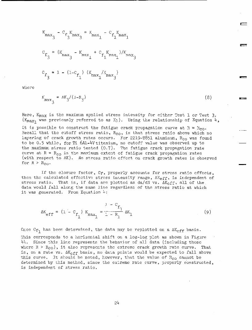
max3 f max3 max 1 f 1max1

Cf = (K - Km + C K max1)/Kmax3

max ( max1 max 1 a3 1 3

Cf 1- (1-Cfl) (K /KC3 f maxI max3=

where

K max3 AK 3/(-R ) (8)

Here, Kmax is the maximum applied stress intensity for either Test 1 or Test 3.(Kmax 1 was previously referred to as KI). Using the relationship of Equation 4,

it is possible to construct the fatigue crack propagation curve at R = Rco.Recall that the cutoff stress ratio, Rco, is that stress ratio above which nolayering of crack growth rates occurs. For 2219-T851 aluminum, Rco was foundto be 0.5 while, for Ti 6Al-4VVtitanium, no cutoff value was observed up tothe maximum stress ratio tested (0.7). The fatigue crack propagation ratecurve at R = Rco is the maximum extent of fatigue crack propagation rates(with respect to AK). No stress ratio effect on crack growth rates is observedfor R > Rco.

If the closure factor, Cf, properly accounts for stress ratio effects,then the calculated effective stress intensity range, AKeff, is independent ofstress ratio. That is, if data are plotted as da/dN vs. AKeff, all of thedata would fall along the same line regardless of the stress ratio at whichit was generated. From Equation 4:

1- Cf1

AKeff= (l- Cf) K max 1 = AK1 (9)

Once Cfl has been determined, the data may be replotted on a AKeff basis.

This corresponds to a horizontal shift on a log-log plot as shown in Figure44. Since this line represents the behavior of all data (including thosewhere R > Rco), it also represents the extreme crack growth rate curve. Thatis, on a rate vs. AKeff basis, no data points would be expected to fall abovethis curve. It should be noted, however, that the value of Rco cannot bedetermined by this method, since the extreme rate curve, properly constructed,is independent of stress ratio.

24

It has been previously reported (Ref 6) that the crack growth stressintensity threshold is dependent on the stress ratio. Equation 9 predictsthreshold behavior which agrees conceptually with existing data on fatiguecrack propagation thresholds.' Replacing stress intensities in Equation 9with threshold stress intensities:

A AKthAKeffth 1-R ( f-C) (9a)

At R = 0,

AKeffth AKth (i - Cf ) (9b)tho o _

where AKth° is the applied stress intensity range threshold at R 0. As

described earlier, AKeffth is a constant if Cf properly describes the crack

closure behavior. Therefore, we can write

I-R- (l - C AKth( - C (10)

o 0

or:

AK = AKth (1 - R) (10a)

so that the threshold value for any value of R is given in terms of the thres-hold value at R = 0 for all values of R < Rco. For R > Rco, AKth = AKeffth.These results are shown schematically in Figure 45.

These techniques will now be considered utilizing actual test data.Figure 46 is a plot of da/dN vs. AKb for two periodic overload tests. In eachcase, a straight line has been drawn which represents the predominant mass ofdata over the range of 10-6 to 10-5 inch/cycle. Both of these tests were runat R = .05. The above analysis can be modified to give an expression forCf. In this case:

AK2 -AK1Cf .05 (O/L) 2 AK2 - (O/L) 1 AK1

25

Choosing 3 x 10- 6 as the crack growth rate for calculating the AK's,AK, = 8.7, AK2 = 12.6 and Cf. 0 5 = .33. This value is within the range of

measured values of Cf at R = 0.05 for the 2219-T851 aluminum data obtainedduring this program. Measured values of Cf ranged from 0.28 to 0.55, asshown in Figure 100.

3.2.2 Ti6Al-4V Titanium Test Results

Like the aluminum tests, the objectives of these tests were to obtaindetailed crack growth and crack closure measurements during and subsequent to

the application of overloads. The titanium test data were more difficult toanalyze than the aluminum data. This was principally due to the data scatterwhich seems to be inherent in the titanium material. This will becomeapparent after reviewing some of the data presented here.

Single Discrete Overloads - These tests were performed in the samemanner as the equivalent aluminum tests. Subsequent to the application of anoverload, the behavior of the crack growth on the specimen surfaces was some-what erratic. Figures 47 and 48 present overall a vs. N curves for titaniumCTB specimens subjected to overloads with O/L values of 1.5 and 1.8 respec-tively. Again, this type of data plot is not useful as an analytical tool.Figures 49a through 49f show detail plots of a vs. ANs for the 18 overloadsequences in Figures 47 and 48.

Several observations can be made. The crack growth behavior sub-sequent to each overload typically exhibits an initial slow rate whicheventually becomes approximately equal to the constant amplitude rate. Of the18 sequences presented, only three exhibit delayed retardation. During thestabilized crack growth portion, the rates are nominally constant amplituderates. Attempts to plot the normalized crack growth rate function, the ratioof measured to calculated constant amplitude crack growth rates, fn, werefruitless. This is because, although the general growth behavior is uniform,the calculated rates exhibit excessive scatter. The general trend of thedata indicate that, as the stress intensity increases (crack length increases)the number of delay cycles decreases. This is in direct contrast to thealuminum results. Delay cycles vs. the stress intensity caused by the over-load, KmaxOL, and vs. the difference between the overload stress intensity

and the baseline stress intensity, Kmax, are presented in Figure 50. It canbe seen that delay cycles decrease as stress intensity increases, but thatneither of the parameters correlates the data. The plane stress plastic zoneradius caused by the overload is shown for each sequence (Figure 49). For thecases where the cracks are relatively short, these values are quite small.The plane stress radii nominally describe the point where the crack growthrates are stabilized. It is interesting to note that, for all of thesequences, plane strain conditions predominate but that a plane stress plasticzone best describes the crack length affected by the overload. Pertinent datafor all 18 overload sequences are presented in Table 4.

26

The stress intensity at which stable tear begins is given in Sub-section 3.5 as 72 ksi Vin. Only the last two events listed in Table 4 exceedthis value. Even so, the behavior of these data appears reasonable when com-pared with the other data.

Single Periodic Overloads - Six titanium compact tension specimenswere subjected to single periodic overloads. Three specimens were subjectedto overload ratios of 1.8 and the balance to overload ratios of 1.25. Thecrack length vs. cycles results for these tests are presented in Figures 51and 52. Figure 51 shows that, for O/L = 1.8, when the frequency of occurrenceof the overload is increased from one application for every 1000 low-loadcycles to one application for every 500 low-load cycles, the life of the spe-cimen is approximately halved. This implies that the overloads contributesignificantly to the crack growth behavior. Conversely, for O/L = 1.25 (Fig-ure 52), when the frequency of occurrence is halved, there is no significantchange in the life of the specimens. (In this case, the lives seem to beslightly longer.) These test results indicate that the effects of the over-loads are independent of frequency of occurrence or do not affect the crackgrowth rates at all.

Figure 53 shows that the overloads (O/L = 1.25) have negligible effecton crack growth rates. In this figure, the average crack growth rate (includ-*ing the growth due to overloads) is plotted against the stress intensity rangefor the baseline loading. The crack growth rates obtained from equation lcfor the baseline loading are also shown. Although the actual rates are slightlylower than those obtained from Equation 1c, the differences are generally quitesmall. For the range of data shown in Figure 53, and using a frequency ofoccurrence of 50 cycles, the crack growth between the overloads ranges fromabout 10% of the plane strain plastic zone radius produced by the overloadsat the low end of the data to about 25% at the high end. The overloads shouldhave the greatest influence on the average crack growth rates when the growthbetween overloads is the smallest (at the low end of the data.) However, itcan be seen that this is where the data most closely agrees with Equation 1c.The conclusion obtained here is that when the overload ratio is 1.25 and thefrequency of occurrence exceeds 50 cycles, the overloads have negligible effecton crack growth rates.

Figures 54 and 55 show that this is not the case when the overloadratio is 1.8. There, the average crack growth rate is plotted againstAKb and AKOL respectively. It can be seen that the measured crack growthrates are always less than those calculated from Equation 1c. Referring toFigure 54, the actual rates range from about one third to about two thirds ofthe calculated rates. Interestingly, these figures show that the absolutevalue of the overload is more significant than .the frequency of occurrence ofthe overload. For example, in Figure 54, the data for the two specimens wherethe overload is 1440 lb are closely grouped even though the frequency ofoccurrence of the overloads differs by a factor of two. Where the overloadsare 1870 lb, the crack growth rates are measureably lower.

27

Using the method described for the aluminum data in Subsection 3.2.1

to determine the crack closure factor (Eq 7) at a crack growth rate of 4 x io-6

inch/cycle, the following results are obtained. For the cases where

POL = 144o lb and 1870 lb, Cf = .28 and .38 respectively. The value of .28is low for this material, but the value of .38 agrees closely with the valueobtained in Subsection 2.4. The difference (.28 - .38) is explained by theamount of crack growth relative to the plastic zone radius. For POL = 1440 lb,

the average growth between overloads is 29% (N = 500) and 57% (N = 1000) ofthe plane strain plastic zone produced by the overloads. As described inSubsection 3.2.1, the growth between overloads must be small relative to theaffected crack length for the values of Cf obtained in this manner to bevalid. For POL equal to 1870 lb, the growth between overloads is less than20% of the plane strain plastic zone radius. In this case, the calculatedvalue of Cf is expected to be more accurate.

3.2.3 Interactions of Single Overloads

The effect of single overload interactions, where additional over-loads are applied before the effect of a previous overload has died out, hasbeen investigated in two different ways. First, a number of the periodicoverload tests were single periodic overload tests in which a specific over-load was repeatedly applied after a particular number of lower loads had beenapplied. These tests are discussed in other sections of this report. One ofthe important conclusions reached from these tests was that, if the number oflow loads between overloads is sufficiently small, the closure load is thesame as if a large number of overloads had been applied and the closure loadis stable.

The second approach was to utilize tests in which another overloadwas applied while the crack tip was still in the vicinity of the originaloverload. Figures 56a and 56b are crack length vs. cycle plots for one ofthese tests. Figure 56a shows an event in which a single overload wasapplied. Figure 56b shows five additional events. In three of the eventsshown in Figure 56b, a second overload was applied after the crack grew 0.006inch from its length at the time of the first overload application. The re-maining two events had the second overload applied after 0.010 inch of growth.

In viewing Figure 56, it is difficult to draw any quantitative con-clusions about the effect of the second overload. It is originally expectedthat closure load measurements of these tests would prove informative but,as discussed in other sections, closure load measurements after single over-loads cannot be made effectively. Figures 57a, b and c present crack growthrate data for the events shown in Figure 56b in which the overloads wereseparated by 0.006 inch. In two of these figures (57b and c) the second over-load seems to have perturbed the crack growth rate pattern. However, for thereasons discussed in Subsection 3.2.1 concerning data scatter, quantitativeuse of this information is difficult. A similar test which shows the sametrends is shown in Figure 58.

28

Figure 59 shows a test result for a test in which a slightly differentapproach was tried. First, a single overload was applied and crack length vs.cycle data was collected (circles). The baseline loading had a stress ratioof 0.7 and the overload factor was 1.25. This was followed by a load sequencein which an overload was applied every 2000 cycles (squares). Two thousandcycles were chosen since it appeared that after 2000 cycles, the crack wouldpenetrate well into the plastic zone produced by the overload. Finally, justthe low loads were applied and the crack growth rate was allowed to returnto its constant amplitude value (triangles). Once again quantative conclu-sions are difficult to reach, but it appears that no retardation occurs forthe single overload, while the repeated overload causes significant retarda-tion (a crack growth rate reduction of 40%).

Titanium data were not included in this section since the affected cracklength is too small to be observed and plotted. It appears that inter-action effects must be evaluated by an inverse approach. That is, the datagenerated should be used to check a hypothesized model, rather than bequantitatively evaluated.

3.3 MULTIPLE OVERLOAD TEST RESULTS

3.3.1 2219-T851 Aluminum

The effects of multiple overloads on subsequent crack growth wereexamined. The test matrix was developed in order to examine three possiblesituations for both materials investigated. The first was to determine theeffect on subsequent crack growth rates of the application of many overloads.Here, many means that enough overloads are applied so that stabilized crackgrowth conditions exist during the overload applications. The second was todetermine the effect on subsequent crack growth of the application of a fewoverload cycles. Finally, tests which were essentially two-level block load-ing were performed.

For the three situations investigated, up to three different overloadratios were used for each of the two materials. In most cases, the stressratios for the two stress (load) levels were maintained at or near zero. Insome of the sequences, the minimum stresses (loads) were not necessarily closeto zero and/or equal for both stress levels. Table 5 presents the test matrixfor all multiple overload tests performed on both materials.

In this section, crack closure behavior has been utilized to explaincertain observed behavior.

Stabilized Overloads - A number of tests consisting of many overloadcycles followed by many low level loads were run. The number of loads at eachlevel was large enough so that stability was reached within that portion ofthe load sequence. That is, each of the steps in the two step load sequencecontained sufficient cycles so that the crack growth rates reflected constantamplitude loading conditions.

29

The primary purpose of these tests was to investigate the transientconditions during the low load sequence as the crack growth rate varied fromfully retarded to unretarded (constant amplitude). This transient behaviorwas far less difficult to observe than was the transient behavior in a singleoverload test. Typical test results for the 2219-T851 aluminum are shown inFigure 60. Once the load has dropped, the variation in rate is monotonic.This is not always the behavior with single overload tests. (See Subsection

3.2.) The highly transient behavior described in Subsection 3.2 does notoccur because the large number of overloads has caused a stable closure valueto be produced. Thus the monotonic variation in rate is simply a manifesta- -

tion of the monotonic variation in closure level, from a value associated withthe high load to a value associated with the low load. This can clearly beseen in Figure 61, which represents the results of a test in which the base-line loading was at a stress ratio, R, of .5. In Figure 61a, the entire a vs.N plot is shown. Figures 61b and c focus attention on a single event in thattest. Figure 61b presents the crack length record for that event and Figure61c presents the applied loads and closure load measurements for that event.The upper and lower bumps called out in Figure 61c are described in the sec-tion on closure measurements. We associate closure with the upper bump only.Thus Figure 61c shows that the closure load rises during the initial portionof the overload sequence, stabilizes, and then drops monotonically duringthe low-load sequence to a stable level associated with that low-loadingcondition.

Note that, for the closure load to return to a low value, the numberof cycles and the change in crack length since the overload is significantlylarger than any comparable measurement on the a vs. N plot (Fig. 61b). Thenumber of cycles to return to the lower closure value is approximately 25,000(362,000 - 333,000) and the corresponding change in crack length is .085 inches(1.29 - 1.205). However, from the a vs. N plot, there is a sharp change inrate to an apparently unretarded condition at a crack length change of about.007 inches and a cycle count of about 15,000. Although the data taken afterthe overload in this test is a little too sparse to construct detailed crackgrowth rate plots in the vicinity of the overload, other tests indicate thata plot of da/dN versus Aa since the overload would yield an estimate for theduration of the effect of the overload of .003 to .020 inch for this case.An example of this is given in Figure 62a and b in which the estimates of thiscritical length would be .004 and .012 respectively. Thus we see that thedetermination of the duration of the overload effect (Aa*) is dependent on themethod used to determine it.

Note that the manner in which the closure load returns to its constantamplitude value in Figure 6 1c is quite complex. Therefore any model thatrepresents this closure variation in a simple fashion (such as a linear or para-bolic variation with Aa) will only be an approximation of the behavior shownin Figure 61c. Thus for a model to be meaningful as a predictive tool, it

will be necessary to choose Aa* in a manner compatible with the assumed

30

variation of the closure load, and in such a way as to yield a match in dataand predictions. The proper method, as far as a predictive model is concerned,is to use a value of Aa* which, in conjunction with the variation in closureload assumed, yields the correct average rates in the transient region andthus a good life prediction.

The parameter Aa* is not simply a single value but varies with theparameters of the test. Many previous investigators have assumed that Aa* isproportional (or equal) to the plastic zone radius as determined from the

Z i Kmax0L• 2 •

maximum value of the overload. That is, it is assumed that As*~ 2 (y )

However, arguments based on the fact that residual compressive stresses play animportant role in crack growth interactions would indicate that an appropriaterange of stress intensity might be the correct variable.

In order to ascertain the correct variable, data for measured Aa*values was gathered and compared to plastic zone radius calculations using avariety of stress intensity variables. These variables are shown schematicallyin Figure 63. In that figure the solid lines represent stress intensitiescaused by applied loads and the dotted lines represent stress intensitiescalculated using the closure loads. In Figure 63a, the three possible per-tinent variables for a two-level test with the same minimum stress intensityin each are indicated.

In Figure 63b, two additional possible controlling variables are indi-cated for those tests in which the minimum stress intensity is different foreach loading sequence. One of the additional variables (KmaxOL - Kmin)

arises simply because of the presence of the second minimum load. The otheradditional variable indicated in Figure 63b occurs because the closure load,.and therefore Kc, variation might follow the pattern established by the dottedline marked II. For that possibility, the final effective range in stressintensity for the overload is determined by Kmin/KmaxoL rather than KminOL/

KmaxOL. That is, the reduction to a lower minimum load is effective immedi-

ately. There is evidence of this behavior in other phases of the program (seeSection 4).

The five possible combinations of pertinent variables and the result-ing plastic zone equations are given in Table 6. Table 7 presents a compila-tion of data and analysis from eleven different events. Overload ratioswere 1.5 and 1.8, stress ratios for the low loads were .05 and .5, andconstant-minimum and different-minimum loads for the overloads and base loadswere used. Measured values of Aa* were determined from Aa versus N plots such

_1/K 2as Figure 62a. A plastic zone radius size, p :-- , was calculated with

each of the trial variable stress intensities substituted for K. The para-meter .25p is listed in three of the cases, simply to maintain all the scales

31

used for plotting at about the same value. Plotting the measured Aa* versusa plastic zone calculation containing the correct variable should produce astraight line dependence of Aa* with py.

The data from Table 7 are plotted in Figures 64 through 68. In Fig-ures 65 and 66, two distinct trends are present, indicating that AKOL and(KmaxOL - Kc 1 ) are not appropriate stress intensity variables for determining

Aa*. An examination of the basic data used for these two figures indicatesthat the steeper sloping line segment is associated with tests with different,minimum loadings for the two load sequences. In addition, we note in Figure 66 =

that there appears to be a tendency toward two distinct lines, and that thesteeper line is associated with high stress ratio tests. The remaining twoplots (Figures 64 and 68) both indicate an approximately linear variationbetween the calculated and measured values. However, it appears that the EMplot using (KmaxOL - Kcll) (Figure 68) has the least scatter. The reason for

the difficulty in clearly discerning which of these two variables,(KmaxoL - Kc 1I) or KmaxoL, is more important is that the range of (KmaxOL -

KclI) was only .4 to .6 times Kmax for all the tests considered. In Subsection

4.1, it will be shown that the use of KmaXOL in calculating the affected

crack length (plastic zone) is straightforward and provides a good fit to thedata for the mathematical model developed under this program.

3.3.2 Ti 6A1-4V Titanium

As in most of the tests run in this program, it was more difficult toanalyze the multiple overload titanium test results than it was to analyzethe aluminum test results. This is due to the apparent increase in datascatter in titanium, the significantly smaller plastic zone sizes in titaniumas compared to the aluminum, and the increased difficulties with the closuremeasurements as described in Subsection 2.4. It was therefore necessary torely heavily on information from the aluminum tests during the development ofthe predictive model.

This is a reasonable approach and is supported by data typified inFigure 69. Figure 69a is a crack length vs. cycle plot for a two-level testwith a baseline stress ratio equal to 0.5, an overload factor of 1.5 andequal minimum stresses in both segments of the load sequence. Two distinctevents are shown. Figure 69b presents the applied loads and the measuredclosure loads for this test. Note that, after the overloads were applied,closure load monotonically decreases from a high value associated with theoverload to a lower value associated with the baseline loading. This type ofresponse is identical to that which was observed for similar tests in alumi-num. (See Fig. 61c.) However, the details of the manner in which theclosure level returns to the lower level are quite different for the two eventsshown. This implies that attempts to model the closure variation using actualclosure data would be quite difficult.

32

Although significant crack growth retardation is apparent in both thecrack length vs. cycle plot and, indirectly, in the closure measurements, thedistance over which the retardation is effective is quite small. This willbe even more apparent in subsequent figures. Note that the closure loadsmeasured before the overloads appear to be higher than the steady state re-sponse after the overloads. It is felt that this is simply a manifestationof problems in measuring closure and not indicative of any real materialresponse.

Some of the problems encountered with closure measurements in thetitanium can be seen in Figure 70. Figure 70a shows the crack length vs.cycles plot for a two-level titanium test, Figure 70b is a similar plot of asingle event in that test, and Figure 70c shows the applied loads and mea-sured closure loads for that test. Retardation is seen in the crack length vs. EMcycles plots. However, there is too much scatter in the closure measurementsto arrive at any quantitative interpretations. Note that, even prior to theoverload, there is considerable scatter in the closure load measurement. Interms of the maximum load, this scatter is not excessive (%15%) but, in termsof the closure load itself, the scatter of approximately 30% causes an enor-mous problem of interpretation.

Figure 71 presents detailed plots of crack length vs. cycles for asingle test specimen. The baseline loading had a stress ratio of .05, theoverload factor was 1. 5 and different numbers of overloads were applied foreach of the eight events. The figures show the growth after each set of over-loads. The large number of events in a single test is possible because of thesmall interaction diktance after an overload for the titanium material. Sig-nificant increases in the amount of retardation still occurred as the number ofoverload cycles was increased past fifty. Note, however, that we cannot reallysee a retarded growth, but that what we see in these plots is a "delay."

This is almost certainly a result of the measuring scale not being sufficientlyfine. For example, had the scale for the aluminum data been sufficientlygross, all we would have seen would have been a "delay" as well. Thus it isimpossible to measure Aa* as was done for the aluminum data. As a result,conclusions reached regarding appropriate stress intensity variables to con-trol Aa* on the basis of aluminum data have to be assumed to be valid fortitanium as well.

Figures 72a through 72h show sequences similar to those of Figure 71.However, these data are for a test in which the baseline loading had a stressratio of 0.3 and the number of overloads applied decreased as the crack grewlonger, rather than increased as was the case in the previously discussed test.Here again, it can be seen that there is more retardation with 50 overloadcycles than with 20 but, in addition, a value of Aa* could be discerned withthe larger number of overloads. That is, there does seem to be an identifi-able location where there is a significant change in crack growth rate.That this point is discernible in this test may be attributed to the fact thatthe maximum overloads are approximately 40% higher than in the previous test.

33

As an additional point, the fact that a value of Aa* is discernible in the

tests with a large number of overloads opens the question of whether increas-

ing the number of overload cycles affects the degree of retardation or the

duration of retardation.

Since the overloads are approximately 40% greater in magnitude for the

data of Figure 72 than for Figure 71, the overload plastic zone would be

approximately doubled. Therefore, larger values of Aa* are to be expected.

However, a casual inspection of the data reveals even larger values of Aa*

than those which were expected. The implication is that Aa* increases as the

number of overloads increases. In this case, the duration of retardation

would be a function of the number of overload cycles. The material cyclicstrain hardening or softening characteristics might also contribute to this

effect. It seems more likely, however, that the degree of retardation might

be altered by additional overloads. It will be shown in Section 4 that when

Aa* is assumed to be the plastic zone created by the overload(s), regardless

of the number of overloads, it yields a generally good definition of the

interacted crack length. Based on this assumption it follows that the number

of overloads controls the degree, but not the duration, of retardation.

Because of the difficulties associated with the analysis of the tita-

nium test results, the modeling approaches used for aluminum were applied to

the titanium test results. The model was verified by comparing the gross be-

havior of the titanium test results to the results predicted by the model.

This procedure is discussed in Section 4. Generally, this approach produced

satisfactory correlation.

3.4 VARIABLE AMPLITUDE TESTS

Variable amplitude tests were performed on specimens fabricated from

both materials. These tests utilized block program loadings with variations.

The blocks were composed of three or four layers, and were arranged in high-

low, low-high and randomized sequences, with all of the minimum loads equal

to or nearly zero. Each loading block was identical to the others in a given

test. Variations on the basic loadings included maintaining all of the mini-

mum loads at some elevated (greater than zero) value with occasional excur-

sions to zero load.

One center cracked panel specimen of each material was subjected to a

fighter spectrum as defined in Table 5 of Reference 7. The limit stresses of

30.9 ksi for 2219-T851 aluminum and 61.9 ksi for Ti 6Al-4V titanium shown there

were also employed in this program.

These tests were performed as an aid in the verification of the math-

ematical model developed during this program. As a result, very littleanalysis of the data was performed.

Table 8 presents the test matrix while Table 9 presents the spectra

employed for these tests.

34

3.5 EFFECTS OF UNDERLOAD AND COMPRESSION SPIKES

A few specimens were tested to obtain some understanding of the effectof underioad or compression spikes. An underload is defined as a reduction inthe minimum load (or stress) such that its minimum value is greater than, orequal to, zero (tensile). The test program included compression (underload)

spikes only, tensile overloads followed by compression (underload) spikes and,to a limited extent, tensile overloads preceded by a compression (underload)spike. Table 10 presents the loading conditions employed.

Underloads - The test plan originally included some compact tensionspecimen tests to investigate the effect of compressive loads on crack growthbehavior. However, preliminary tests and some reflection indicated that theresults might be difficult to interpret. It can be seen that, for any speci-men configuration, once the crack surfaces are in contact, a cracked specimenbehaves like an uncracked specimen and the important load parameter is thestress, not the stress intensity factor. The load at which the entire crackis closed will be a complex function of specimen geometry and crack length.No method currently exists to determine the load at which the entire crackcloses. In the case of the compact tension specimen, there is a tendency forthe crack tip to open when compression loads are applied. This is especiallytrue for long cracks (large values of a/W). In this case, proper characteri-zation of crack growth phenomena in terms of either stress or stress intensityis currently beyond the state-of-the-art.

As a result, an alternate test procedure was adopted. The new testswere performed using a baseline loading with a stress ratio greater than zeroso that the minimum applied load was significantly greater than zero. Then,occassional or multiple excursions to approximately zero load (referred to asunderloads) were applied. It was felt that, in tests of this nature, theunderload(s) would have the same general effect on subsequent crack growthduring the baseline loading as a compression load(s) might have if the speci-men had been a center-cracked panel. For example, an underload with R = .05should have the same qualitative effect on tests with a baseline R = .5 ascompressive loads have on tests run with a baseline R = .05. Since the majorportion of the crack surfaces are not in contact during these tests, inter-pretation of the test data in terms of stress intensities is considered to berational.

Six specimens, three each of titanium and aluminum, were tested in this

manner. All six specimens had a baseline loading with R = .5. Two each ofthe aluminum and titanium specimens had additional single cycles of loadingwith an underload of zero and an overload ratio of 1.5 superimposed on thebaseline loading. However, the order of loading (underload-overload oroverload-underload) was modified for different specimens. The aluminum testresults are shown in Figures 73 and 74. As noted earlier, a single overloadcycle with an overload ratio of 1.5 does not cause very much retardation in

2219-T851 aluminum. One could argue that there was retardation in the test

35

in which the underload preceded the overload and that there was no retardationwhen the underload followed the overload, but the differences are not signi-ficant. The titanium test results shown in Figures 75 and 76 are slightlymore conclusive. This is due to the fact that single overloads with overloadratios at 1.5 do cause some retardation in titanium. There appears to besome retardation in the test in which the underload follows the overload, butit is certainly quite small. However, the test for which the underloadprecedes the overload shows significant retardation.

The remaining specimens in this series were used to investigate theeffect on subsequent crack growth of a large number of overloads followed bya single underload cycle. The test results for the titanium specimen are

shown in Figure 77 and those for the aluminum specimen are shown in Figure 78.In both these figures, little if any retardation is evident.

In addition to these tests, a single underload cycle was appliedduring the constant amplitude loading of one of the specimens (AD-25-117). Itwas felt that the drop in load could have decreased the closure level and

thereby caused a short period of crack acceleration. As can be seen in Fig-ure 79, no significant acceleration occurred.

Although, only a limited number of underload tests were run, thesetests indicate that:

"* A single underload can change the closure load sufficiently toremove the effects of previous overloads.

"* Although a single underload may reduce the closure load, subsequentconstant amplitude cycling causes the closure load to recoverrapidly enough to eliminate any significant acceleration.

If these observations are extended to compression, we may concludethat compression excursions reduce or eliminate retardation, but do not causesignificant acceleration.

Compression Spikes - Center-cracked panel specimens, suitably stabi-lized against column buckling, were subjected to compression, tension-compression and compression-tension loading sequences. Results from 2219-T851aluminum tests indicate that the application of a single isolated compressionspike has virtually no effect on subsequent crack growth behavior. This con-clusion is substantiated by the test results shown in Figures 80a through 80cand 81. There, crack length is plotted against ANs (the number of cycles sincethe compression spike) for compression spikes ranging from one half to twotimes the maximum baseline tension loading. In addition, the crack length vs.ANs curve, calculated using constant amplitude growth rates and neglecting anyeffect of the compression spike, is plotted for each case. In Figures 80athrough 80c, there is a tendency for the calculated lives to be slightly

longer than the actual lives. In Figure 81 however, the opposite result can

36

be observed. Based on the results of these tests, it was concluded that thecompression spikes had negligible effect on subsequent crack growth in thealuminum.

Figure 82 presents similar results for a titanium panel subjected tooccassional compression spikes. These results seem to indicate that thecompression spikes produce subsequent crack growth rates which are greaterthan constant amplitude rates. In some cases there is an initial perturbationof the data immediately following the application of the compression spike andthe rates are higher than the constant amplitude calculations. The two casesshown on the left side of Figure 82 show this most prominently. However, aftera crack extension of about 0.05 inch (for these two cases), the crack growthbehavior appears to stabilize. The rates in these apparently-stabilizedregions are still measurably greater than the calculated values. This ten-dency indicates that some scatter may be present in the constant amplitudecrack growth behavior for this specimen. The data shown in the right side ofFigure 82 lie somewhat closer to the calculated curves, but still exhibitshorter lives than the constant amplitude calculations. Based on the resultsfrom these two figures, the compression spikes seem to produce somewhat fastersubsequent crack growth rates in the titanium material, but the data are in-sufficient to reach any quantitative conclusions.

Tension-Compression Spike Sequences - Figures 83a through 83c presenta vs. ANs data for aluminum specimens subjected to tension spikes followedimmediately by compression spikes. A calculated constant amplitude crackgrowth curve which neglects any effects of the tension or compression spikesis also shown for each case. The first two cases (Fig. 83a) resulted from theapplication of tension-compression spike sequences where the magnitude of bothspikes was 1.5 times the baseline loading. It can be seen that the actualcrack growth rates are much lower than the calculated rates. These resultsimply that the tensile spike causes a retarding effect on subsequent crackgrowth rates and that the compression spike does not appear to offset theeffects of the tensile spike. It was concluded in Subsection 3.2.1, however,that a single overload, where the overload ratio was 1.5, produced very littleretarding effect on subsequent crack growth rates for the 2219-T851 aluminummaterial. The decreased rates shown in Figure 83a are therefore attributedto scatter and these results are inconclusive. The results shown in Figure83b and 83c are only slightly more conclusive. There, the tensile overloadratios were 1.5 and 2.1 and the compression spikes ranged from 0.5 to 3 timesthe baseline tensile loading. For the cases where the tensile overload is9 ksi (overload ratio = 1.5), the data lie close to the calculated constantamplitude curves.

If the compression spikes had not been included, the tensile overloadwould be expected to cause very little effect on, subsequent crack growthbehavior. The compression spikes by themselves have been shown to produceessentially no effect on the subsequent rates for this material. Therefore,

37

it can be concluded that the combination of tensile overloads followed bycompression spikes have, for the overload ratio of 1.5, very little effect onsubsequent crack growth behavior.

For the three cases where the tensile overloads are 12.6 ksi (overloadratio = 2.1), there is a consistent trend such that the actual lives arealways greater than the calculated constant-amplitude lives. These resultsindicate that the tensile overloads have caused some subsequent retardation.The number of delay cycles are approximately 9,000, 7,000 and 11,000 for thecases where the compression spikes are 3, 12 and 18 ksi respectively. Insuf-ficient data were gathered for single overload spikes alone (where the over-load ratio was 2.1) to quantify the number of delay cycles. It is thereforeimpossible to say how much the subsequent compression spikes influenced theseresults.

It is interesting to note that the number of delay cycles are approxi-mately the same for all three cases and that the stress intensity for thelongest crack length, when the spikes are applied (1.205 inches), was only17% greater than that for the shortest crack length (0.88 inch). It can beexpected that if no subsequent compression spikes had been applied, the num-ber of delay cycles would be approximately the same since K is nominallyconstant. The introduction of the compression spikes did not cause any sig-nificant variation in the number of delay cycles. It can therefore be con-cluded that the subsequent compression spikes either: 1) do not alter theeffects on subsequent crack growth rates of the tensile overload, or 2) anymodification of the tensile overload effects is ifidependent of the magnitudeof the compression spikes, at least for the ranges considered here. It willbe shown in Subsection 4.1.3 that, for these three cases for this specimen(AG-15-10P), the conclusion that the compression spikes have negligibleeffect is correct.

The data for a similar test, performed on a titanium specimen, arepresented in Figure 84. In addition to tension-compression sequences, somecompression-tension sequences were also applied to the specimen. The tensileoverloads were always 1.5 times the maximum baseline loading and the compres-sion spikes were either 0.5 or 1.5 times the maximum baseline loading, Forthe Ti6Al-4V material, single overload spikes having an overload ratio of1.5 do cause some subsequent crack growth retardation. For three of the fourcases, where the compression spike precedes the tensile spike, some initialretardation is present. (The first data point after ANs = 0 shows a cracklength which is equal to or only slightly larger than the value at ANs = 0.)However, the subsequent stabilized crack growth rates are always greater thanthe calculated constant amplitude rates, so quantification of the number ofdelay cycles is impossible. In three of the four cases where the compressionspike was applied after the tensile spike, the first data point after ANs = 0shows that the crack length is greater than the value at ANs = 0. Theseresults indicate that, for the titanium, the application of the compressionspikes tends to negate the retarding effects of the tensile overloads. Again,no quantitative conclusions are possible.

38

It can be concluded that, generally, the application of compressionspikes, either alone or following a tensile overload, have very little in-fluence on the subsequent crack growth behavior in 2219-T851 aluminum. Forthe Ti6Al-4V titanium material, compression spikes seem to accelerate sub-sequent crack growth. When compression spikes are applied prior to a tensileoverload, the results were inconclusive, but where they were applied subsequentto a tensile overload, they tend to negate the effect of the overload on sub-sequent crack growth rates.

3.6 MISCELLANEOUS TEST RESULTS -

3.6.1 Stable Tear

Some of the aluminum specimens tested at high K levels exhibited slowstable tear. This is the phenomenom which occurs when the stress intensityunder monotonically increasing tensile loading approaches the, critical stressintensity of the material, thereby causing a significant amount of crackextension. In order to quantify this stable tear, a crack growth resistancetest was performed on a 2219-T851 aluminum compact tension specimen. Thistest was performed by measuring the crack opening displacement (COD) undermonotonically increasing load until the load vs. COD trace became nonlinear.The specimen was then unloaded sufficiently to produce a new, linear, load vs.COD trace. The load was again increased monotonically until some further non-linearity occurred and the process was repeated. Figure 85 shows the procedureschematically. Each of the linear unloading traces was used to determine thecrack length and maximum stress intensity at each point where the linear un-loading lines intercepted the overall load-displacement curve. In thismanner, plasticity effects were excluded and crack extension was the onlysignificant variable. Since the material thickness was nominally the samefor most aluminum specimens, it is not considered to be a variable here.

It should be noted that the initial crack length prior to runningthe test was measured on the surface of the specimen and was assumed to bestraight and normal to the surface. Subsequent calculations, based on CODmeasurements by necessity, used the same assumptions. In reality, somecurvature of the crack front was present, although no effort was made to in-clude this curvature in the stress intensity calculations. The results areplotted in Figure 86 as Kmax vs. incremental crack extension, Aa, measuredfrom the initial crack length. The total crack length was calculated fromthe COD measurements. The results were extrapolated to an intercept value ofapproximately 30 ksi YTn for Aa equal to zero. This value of K is defined asthe threshold for stable tear, Kst. Since failure occurs at the point wherethe applied stress intensity curve is tangent to the resistance curve (seeReference 8,) the upper bound or maximum value of the apparent critical stressintensity, Ker, is 57.5 ksi VT-

39

The results of this test indicate that whenever the stress intensityexceeds 30 ksi Vrin (Kst) for this aluminum, some stable tear could be expected

to occur. In some cases of single overload applications, the peak stressintensity during the overload exceeded Kst.

Specimen AG-25-6P, a center cracked panel, was subjected to several

single overload applications of 21 ksi with a baseline stress range of 10.0to 0.5 ksi. In all cases, the stress intensity during the overload exceeded

Kst. A visual examination of the fracture surface revealed that, during theoverload, the crack growth along the center line of the specimen exceeded thegrowth on the surface of the specimen. The internal growth is referred to astunneling and is shown schematically in Figure 87. For the cases of long

cracks (KmaxOL approaching Kcr), this difference was relatively large. The

tunneling, defined as at, was measured for five events, using an optical com-

parator. The values obtained from both crack tips were averaged and arepresented in Table 11. Values of at, taken from the resistance curve (Figure

86) for each value of KmaxOL, are also presented and agree closely with the

measured values.

Figure 88 shows a vs. N after one overload application on specimen

AG-25-6P. The data points representing surface measurements are almost flatfrom the point of application of the overload up to about 329,000 cycles,indicating that there is almost no surface growth during this period. Atabout 329,000 cycles, a sudden jump in the surface length occurs which isfollowed by a monotonically increasing a vs. N curve.

The stress intensity during the overload was 36.3 ksi Vi-n-. at a halfcrack surface length of 0.852 inch. From the crack growth resistance curve(Fig. 86) the expected stable tear is 0.008 inch. It was assumed that the

crack front increased by this amount at the centerline of the specimen thick-ness during the application of the overload, to a half crack length of 0.860inch. The dashed curve in Figure 88 indicates the assumed behavior of the

crack tip at the centerline of the specimen thickness. At 329,000 cycles,after the jump in length, the surface length agrees closely with the assumed

centerline crack length.

Figure 89 presents the normalized crack growth factor vs. crack growth

increment subsequent to the overload, for the data of Figure 88. The nor-malized crack growth factor, fn, is the measured crack growth rate divided by

the calculated constant amplitude crack growth rate. When interpretedliterally, the data exhibits an unusual sinusoidal behavior. The dashed line,however, indicates schematically how the crack growth at the centerline of

the crack tip might vary. The crack growth and rate data were of no value foranalysis purposes until after the surface lengths agreed with the internallengths. Prior to this point, the apparent surface crack growth rate was

zero.

4o

These large crack extensions were generally accompanied by extensiveplasticity near the crack tip. The extent of plasticity was observed to beconsiderably greater than values obtained from the Irwin plastic zone expres-.sion (Reference 9). It was apparent upon reviewing data such as this that itwould be very difficult to define the actual, nominal crack tip growthbehavior.

A crack growth resistance test was also performed on a Ti6Al-4Vspecimen. The results, shown in Figure 90, indicate that Kst is approximately72 ksi iiw: (extrapolated) and that the upper bound or maximum value of Kcr isabout 81 ksi VinT. Only a few events involved stress intensities in excess of72 ksi V§i-n., so stable tear was not a problem for the titanium.

3.6.2 Thickness Effects

Although a detailed evaluation of the effects of thickness variationon fatigue crack growth retardation is beyond the scope of the present study,a few tests of .75 inch thick Ti 6A1-4V titanium were run for comparison withthe .25 inch thick material used in the bulk of the program.

The results of the first test on .75 inch (instead of .25 inch)material are shown in Figure 91, along with test results from a .25 inchspecimen. Both specimens were sized identically (except for thickness) andthe applied loads were scaled by the thickness. In each test a periodicseries of 100 overloads followed by 1000 low loads was applied. Care wastaken to start the loading sequence at about the same location in eachspecimen.

As can be seen, the two test results match quite well. The lowerrate at the longer crack lengths in the thin specimens can be explained interms of decreased environmental susceptibility in plane stress. This sametrend has been observed in constant amplitude test results of other investi-gators. In fact, this test is very similar to constant amplitude testing inmany ways. It is essentially a steady-state test in which the closureload remains constant throughout the test. This constant-closure phenomenomwas demonstrated for this type of periodic loading early in the program.Thus, the fact that the thickness does not significantly affect the retardedcrack growth is not surprising in light of the general lack of a thicknesseffect for constant amplitude loadings. From this test result one mighthastily (and apparently incorrectly) conclude that the thickness does notaffect the closure loads. Actually, aproper conclusion is only that thestable or quasi-stable closure levels do not depend on thickness. Obviously,in constant amplitude loading, the closure level reached and maintained cor-responds to the stable level reached after a large number (>100) of loads areapplied. Since the crack tip does not grow significantly (% plastic zoneradius) between overloads in the test shown in Figure 91, the (quasi-stable)closure level reached also corresponds to the level reached after a large

~41

number of loads are applied. The results shown here simply support theresults of constant amplitude loading which indicate that the closure levelis not a function of thickness. The effect of isolated overloads, however,does appear to vary significantly with thickness.

This can be seen in Figure 92, where two corresponding tests of .25and .75 inch thick material are compared. The test specimens were not identi-cal. However, each individual loading sequence was initiated at nominallymatching stress intensity factors. This was accomplished by choosing appro-priate crack lengths for each loading sequence in the .75 inch specimen.The surprising observation of the comparison in Figure 92 is that there ismore (or at least longer periods of) retardation in the thick specimens thanin the thin. This result is exactly the opposite of what was anticipated.

To confirm the results of the previous test and to remove the con-founding effects of varying the number of overloads, the test of specimenTD-25-106, in which single 1.8 overloads were applied, was reproducedon a thick specimen. Once again the test specimens were different but thestress intensities at each overload were matched. As can be seen in Figures93 through 96, the conclusion is the same; the thick specimen shows morepronounced retardation than does the thin specimen.

In each of these figures, a vs. N for a particular overload in the.75 inch material has been plotted along with the data from the test ofTD-25-106. It is important to note that although the retardation in the thickand thin specimens is different, the rates in each thickness match once aconstant amplitude rate is attained. This can be seen by the matching of theslopes of a vs. N. It confirms our previous conclusions and the fact that thetest is being run properly.

Since constant amplitude testing and Figure 91 imply that the satura-tion closure levels are invariant with thickness, and since Figure 92 containsload sequences that have as many as 2000 overloads and still show a variationin retardation (or at least a variation in the return to baseline) with thick-ness, one must conclude that the closure stress variation as the crack growsmust be different in the thick and thin sheets. It is not yet clear whetherthe resumption of the constant amplitude (saturation) closure level occursat the same Aa* or at a different Aa*. However, it is important to notethat, at least for those cases where the number of overloads is large, theinitial closure load must be the same. Obviously, the other end point, theconstant amplitude closure level, must also be the same.

3.6.3 Tensile Tests

Tensile tests to obtain material mechanical properties were conductedusing the equipment described in Section 2. The results are self-explanatoryand are presented in Table 12.

42

3.7 SUMMARY OF TEST RESULTS

Under constant amplitude conditions, crack growth rates are functionsof both stress intensity range and stress ratio for both materials. Thestress ratio cutoff was 0.5 for 2219-T851 aluminum while no cutoff was observedfor R up to 0.7 for Ti6Al-4V titanium. No effect of stress or load level oncrack growth rates was observed for either material over the ranges tested.At the same values of stress intensity range and stress ratio, the aluminumcrack growth rates were approximately three times those for the titanium. Allthree basic specimen geometries yielded comparable crack growth rates although =

the compact tension specimen yielded erroneous results for negative stressratios.

Single overload cycles less than, or equal to, 1.5 times the baselineloading have negligible effect on subsequent crack growth rates for 2219-T851aluminum. The same is true for overloads equal to 1.25 times the baselineloading in Ti 6AlI-4V titanium. At a given overload ratio and baseline stressratio, delay cycles increase as a function of crack length and therefore,stress intensity for aluminum. For titanium, the opposite result was observed.For the methods used to analyze the data subsequent to a single cycle overload,the affected crack length was approximately equal to the plane strain plasticzone for aluminum and to the plane stress plastic zone for titanium. Delayedretardation was not evident in either material.

Single periodic overload tests can be employed to obtain an approxi-mate value of the closure factor. These data can be used in conjunction withconstant amplitude data to obtain the extreme crack growth rate curve, whichis independent of stress ratio effects.

In tests where a single overload cycle was applied before the effectof a previous overload had disappeared, the results were inconclusive. Forthis type of test, the aluminum exhibited extensive scatter and the titaniumwas impossible to analyze due to the extremely small affected crack lengths.

Where multiple overloads are applied, the degree of retardation ofsubsequent crack growth increases as the number of consecutive overload cyclesincreases, up to a limiting number of overload cycles. Beyond that limit, theaddition of overload cycles produces no additional retardation. The durationof retardation subsequent to one or more overloads appears to be independentof the number of overloads. The duration of retardation (affected cracklength) is a function of the plastic zone caused by either the maximum ampli-tude of the overload or by the difference between the maximum amplitude of theoverload and the closure level. Closure data were easier to read for multipleoverload conditions than for single overload conditions, but still possessedconsiderable scatter.

43

Single underload or compression spikes, either applied alone orpreceding or following a single tensile overload cycle, had very littleinfluence on subsequent crack growth for 2219-T851 aluminum. However, asingle underload negated the retarding effects of multiple preceding tensileoverloads. In the Ti 6A1-4V titanium material, single underload or compres-sion spikes caused slightly accelerated subsequent crack growth rates. Theeffect of a single underload or compression spike which preceded a tensileoverload cycle had little effect on the retardation caused by the tensileoverload. When a single underload or compression spike followed one or moretensile overloads, it significantly reduced the retarding effect on subsequent

crack growth of the overload(s).

Measurable stable tear began at a stress intensity level of about30 ksi VTn for 2219-T851 aluminum and at about 72 ksi in. for Ti 6A1-4Vtitanium. Stable tear tends to manifest itself as internal tunneling with,in many instances, negligible surface growth. The limiting values of criticalstress intensity for the 1/4 inch materials are 57.5 ksi /177. for aluminum and81 ksi VE7 for titanium.

Varying the material thickness does not appear to affect stabilizedcrack growth behavior for either material, but may influence transient

behavior.

44

4 - MATHEMATICAL MODELING

Several mathematical models have been developed in an attempt todescribe crack growth interaction effects. Perhaps the most widely known arethe Wheeler model (Ref. 10) and the Effective Stress Retardation model devel-oped by Willenborg, et. al. (Ref. 11). Both of these models modify the crackgrowth rates subsequent to overload(s) in order to account for retardation.The Wheeler model modifies the crack growth rate such that the retarded crackgrowth rate is equal to the unretarded crack growth rate times a parameter C

p

ret CAP

where

m (12)p (a) fora+p<aCp = ap - a f r a + p<a p

and C =1. for a + p ? a (13)p p

Here, p is the plastic zone radius caused by the current loading at the currentcrack length a. The parameter ap represents the farthest extent of the elastic-

plastic interface caused by a previous overload. The empirical exponent m isdetermined from spectrum test data by trial and error. It was intended that mbe a material constant and, once determined, be spectrum independent. However,several investigators (i.e., References 5 and 7) and results of work on thiscontract have shown that m is spectrum dependent.

The Effective Stress model accounts for interaction effects by modifyingthe applied stress range to an effective stress range:

AS =Sme - S min (14)eff maeff mmeff

where

Smaxff max Sred

145

and

Si = S - S (14b)mn min rede ff

where

red = Sap - Smax (14c)

The magnitude of S is that stress required to set the plastic zone caused byap

S ap (acting on the current crack length, a) equal to the elastic-plastic inter-

face, ap, caused by a previous high load. Both ASeff and Smineff are con-

strained to be L zero. In some loading sequences, this retardation modelpredicts the crack growth under spectrum loading fairly well. However, Figure97 shows a typical case where the prediction is very unconservative. An addi-tional shortcoming of this model is that an overload will cause crack arrestfor the subsequent loading if the subsequent loading is equal to or less thanhalf the magnitude of the overload (O/L = 2). This has been demonstrated tobe incorrect (Ref. 5). A modification to the model, developed by Gallagher(Ref. 12), makes the overload factor, O/L, a variable. This has been shownto produce improved predictions.

The greatest shortcoming of both of these models (Wheeler and EffectiveStress) is that they do not differentiate between the effect on subsequentcrack growth of single and multiple overloads. As described in Section 3 ofthis report and by others (References 5, 13 and 14), this effect can besignificant.

4.1 CRACK CLOSURE MODEL

Elber (Ref. 15) demonstrated the phenomenon of crack closure andsuggested that variations of the crack closure stress might be responsible foror help to explain crack growth interaction effects. Based on this premise, amathematical model, using crack closure as a basis, has been developed. Themodel uses the variations in crack closure to predict crack growth interactioneffects during spectral loading.

4.1.1 Crack Closure Concepts

Elber (Ref. 15) showed that cracks subjected to tension-tension loadingopen and close when the remotely-applied stress is some value greater than zero.This effect. is shown schematically in Figure 98. Assuming that crack growth(extension) occurs during the increasing tensile portion of a cyclic loadingsequence as proposed by Elber, the pertinent stresses involved in the growthprocess should be the crack opening and maximum stresses. It has been shown

46

(References 15 and 16) that the crack opening stress differs from the crackclosure stress, but for the purposes of this discussion they will be consi-dered to be equal and will be referred to as the closure stress.

Referring again to Figure 98, the effective stress range, AS eff is

equal to the difference between the maximum stress, S, and the closure

stress Sc

ASeff = max - c (15)

Defining the closure factor, CV as:

S (16)Cf S

max

Equation (15) becomes:

ASeff = S ( -C f) (15a)ff maxf

Elber proposed indirectly that Cf is a function of stress ratio, R,

through his equation:

S - S (17)max opU=s SS -S .max min

where S is the crack opening stress, called S *here. Therefore,op c

I- Cf (17a)1 R

which, according to Elber

.5 + .4R (17b)

47

for 2024-T3 aluminum. Therefore:

Cf = 1 - (.5 + .4R) (1 - R) (17c)

Equation (17c) can be inserted into Equation (15a) to produce:

ASeff = Smax [(.5 + .4R) (1 - R)] (15b)

which can be generalized to:

ASeff S max [(l + qR) (1 - R)] (15c)

When Equation (15c) is inserted into a Paris-type crack growth equation, it isreferred to as the Elber growth equation (reference subsection 3.1):

d-da = C ISma (1 + qR) (1 - R) fa n(15d)

dNma

for the case of a through crack in an infinite sheet. This geometry has beenassumed for convenience, but it should be noted that S 7Ta times an appropriatestress intensity magnification factor may be used in any of these equationsfor other geometric configurations.

For the purposes of this model, a Paris-type growth equation wasemployed:

da = AKn (18)dN

= I [Smax(l - R)•] na (18a)

Elber also showed that

n

daN LC [(Smax - c)VTa (18b)

48

For constant amplitude crack growth conditions, equations (18a) and (18b) mustbe equivalent so that:

n n

C [Smax(l - R) ra] =1 C Sma(l- Cf Via (18c)max f

or:

nC1 = C-1R 1(18d)

Cf I

For the case of R = 0,

n

C, = C ] (18e)cf0

where Cf is the closure factor at R zero. Equation (18b) then becomes:

00da r Smax c Sc n

The coefficient C and exponent n have the same values that would bedetermined by using the Paris expression (Equation (18)) to fit crack growthrate data plotted against the actual applied stress intensity range.

Equation (19) is the basis for all crack growth calculations performedby the model. Elber showed that S was a function of S and R during steady-c max

state (constant amplitude) crack growth. If Sc in Equation (19) is defined as

a function of stress ratio, then Equation (19) will predict the effect ofstress ratio on crack growth rates. (It should be noted that the results ofthis investigation indicate that the closure stress is a function of stressratio only and does not appear to be stress-level dependent. That is, theclosure stress is always some percent of the maximum load, depending on what Ris, and does not depend on the absolute magnitude of the maximum load.)Further, if S is defined as a function of the previous load history, then

c

h9

Equation (19) will predict crack growth interaction effects. It remains then,to define S as a function of stress ratio and previous load history, and anyc

other pertinent parameters, so that Equation (19) will properly predict crackgrowth rates for any conditions. The determination of the generalized behaviorof S as a function of load history is the subject of the following section.

c

4.1.2 Application of Crack Closure to Mathematical Model

The discussion of the crack closure model centers around the resultsfor the 2219-T851 aluminum test data obtained during this program. This wasione for convenience since the aluminum test data was more convenient toanalyze and revealed information not readily available from the titanium testlata, particularly in the definition of affected lengths (plastic zones) andthe crack growth within the affected lengths.

After the model had been developed for the aluminum data, the neces-sary parameters were determined for the titanium data, and the model was usedto verify that it properly predicted the crack growth behavior of the titaniumdata. In general, the latter is true and is an indication that the modelemploys the basic concepts necessary for general predictive work.

In the past, it has been suggested that many parameters influence crackgrowth interactions. The most significant parameters were determined from thetest data as far as possible. In some areas, quantitative values were notdivulged by the data and a certain amount of intuition was employed. In allcases, the model was verified by comparing predicted a vs N curves with thetest data. The most significant parameters found during this program were:

"* Effect of R on constant amplitude crack growth

"* Effect of maximum overload stress, SOL, on subsequent retardedgrowth

"* Effect of previous minimum stress relative to current minimum stresson subsequent growth

"* Effect of number of overload cycles, NOL on subsequent retardedgrowth

"* Effect of compression on both constant amplitude and variableamplitude growth.

Constant Amplitude Crack Growth - The crack growth rate equation for2219-T851 aluminum was given as

lO~ [l AK]3.34~

da = 1.96 x 10-9 [(l + .6R) AK] for 0 < R : 0.5 (la)

50

Equation (19) with C = 1.96 x 10-9 and n = 3.34 is

da [S

(3.34

1. .96 x ls/ 1l - C f(9

0

As a convenience, taking K = S VTra and K = Scfmax max c c

da 3.34 BE

= 1.96 x 10 L' (19a)

0

Equations (la) and (19a) are equivalent under the same conditions so that:

KKc -Cf = 1 -- (i - Cf ) (1 + .6R) (1 -R) (20)

max o

Equation (20) is plotted against stress ratio in Figure 99 for the case ofCf = 0.23. This value of Cf was selected so that at R = R = 0.5 (fromf f co

0 0

subsection 3.1.1) in Equation (20), the effective stress range is equal to theapplied stress range. The difference between Cf = 1 and Equation (20),

multiplied by K is the effective stress intensity range AK eff. The dashedmaxef

line on the right represents R, so that the difference between Cf 1 and R

multiplied by K is the applied stress intensity range, AK. It can be seenmax

that Equation (20) crosses the R curve at a value of R = 0.5. The figureindicates that for R < 0.5, the closure stress intensity, Kc3 is higher than

the minimum stress intensity, Kin and AK K - K . For R > 0.5, Kmi eff max c c

is less than Km. so that, physically, AK = AK (Kc = Kin) at R = 0.5 andmin eff c min

stress ratio layering stops at that value of R.

Figure 100 presents Equation (20) using Cf = 0.23, replotted with0

measured crack closure values. It can be seen that the calculated values ofCf lie along the lower edge of the scatterband of the data and indicate that

the calculated value of Cf (0.23) is too low.0

51

E2

Figure 100 also shows Equation (20) plotted with Cf = 0.40. It will0

be shown later that this value provides a better fit to the variable amplitudedata from a predictive standpoint and here, in the figure, fits the measuredclosure values quite well except for R >0.4. It is apparent that the form ofEquation (20) is incorrect. Further, Figure 100 shows that, for values of Rless than -1/3, Cf increases; an undesireable behavior.

Another form for Cf was developed, specifically to describe the crack

growth behavior for negative values of R while at the same time providingreasonable correlation for positive stress ratios. For a stress ratio of -1,

da 2.6 x lo-9(Km) (R = -1) (2)dIN max

and for R = 0, Equation (la) becomes

da 1.96 x io- 9 (K 3.34 (R o) (la)

dN max

so that

Ida\_\dN)R -1 - 2.60.

da = 0 = = 1.327

Similarly, taking the ratio of the crack growth rates, but using the form ofEquation (19):

K K 3.34

SR =-i o R=-Jda max - c R =-1

o [K - K

B = 0 [KLmax K c ]3-30o-2 R=0

52

Since K was defined to be the same as AK at R = 0 and R -1max

(da) - 1 - Cf 3.34

(daB 1-Cf 1.327

dN /R 0 0

Cf =i -1.088(1- c)

and

= 0.347 for Cf = 0.4f

In a similar manner, the C at a positive stress ratio may be obtained. Forf.

R = 0.5, Cf. 0.789. *These values of Cf vs. R were fitted to an equation of.f.

the form:

Cf= Cf. 1 + (Cf - Cf.l) (1 + R)p (21)

where

C = 0.347f-

1

Cf =0.400

p= 3.93

and plotted in Figure 101a. It can be seen that Equation (21).agrees closelywith Equation (19) in the region 0 < R < 0.5. Equation (21) was used to defineCf as a function of R and the resulting closure stress intensities were used

53

in Equation (19a) to calculate crack growth rates. These rates are comparedin Table 13 with those of Equations la and 2, which were generated independentfrom crack closure considerations.

The table shows that the crack growth rates calculated from Equations (19a)and (21) are always less than 5% greater than those obtained from Equationsla, lb and 2 up to a stress ratio of 0.6. The maximum error of 5% is wellwithin the accuracy of the crack growth rate data. As a result, Equation (21)was used to define crack closure as a function of R, so that the effects ofnegative stress ratios and compression stresses are accounted for.

For Ti 6A1-4V titanium, the parameters for Equation (21) weredetermined to be:

C f = 0.332

Cf =0.400

p =3.33

Equation 21 is shown in Figure 101b for the titanium material.

A comparison of crack growth rates as a function of R is shown inTable 14 for Ti 6A1-4V titanium. It can be seen that, for R > 0, the crackgrowth rates calculated from Equations (19a) and (27) are within 2% of thevalues obtained from Equation 1c. For R = -1, the values from Equations(19a) and (21) are about 25% less than the value from Equation 3. Since onlyone titanium specimen was tested to obtain the R = -1 data, the parameters forEquation (21) were selected to provide a good fit to the R > 0 data.

High-Low Loading Sequence - The high-low loading is the sequence mostfrequently analyzed by investigators. Following is a description of how thecrack growth data during the low portion of a high-low loading sequence can beused to determine the closure factor at R = 0, (C ) as well as the affected

f

crack length over which retarded crack growth occurs. Figure 102 shows thecase for many cycles of high stress, SI, followed by a lower stress, S2' For

convenience, the stress ratio for both stresses is taken as zero. It is wellknown that, initially, the crack growth during the lower loading, $25 is retarded.

54

The crack closure model assumes that the closure stress, S , varies as shown.c

Immediately prior to the change in stress, the closure level is the stabilizedlevel, S , associated with S1, and varies as shown through some affected

length, p, to the stabilized value, S c2 associated with level S The

expression defining the variation is given by:

AaBSc =S -(Sc Sc2) ( ) for o < Aa p (22)

1WE

where

S = Generalized closure stressc

Aa = Crack growth since the stress change at a 0

p = Plastic zone radius caused by SI at a°

B = Empirical exponent

By definition, Sc > S c. It will be shown that the crack growth rate following1 2the load change is immediately retarded.. Delayed retardation does not occur.

Previously, it was stated that a value of Cf = 0.4 provided a good0

fit to the variable amplitude aluminum data. This value can be verified andin addition, the parameters p and B may also be calculated. Figure 103 showsschematically how the crack growth rate varies as a function of Aa subsequentto the load change. Immediately after the load change, the rate is (da/dN)l.

This value is used in Equation (19) while at the same time setting Smax = S2,

S S and a = a . For R = 0, S =S C so'that:c c10 c 1 0

da) C[(2 1 fo~ a(n23)- i S= 2 - SI Cf

dN [ 1. f-C0

55

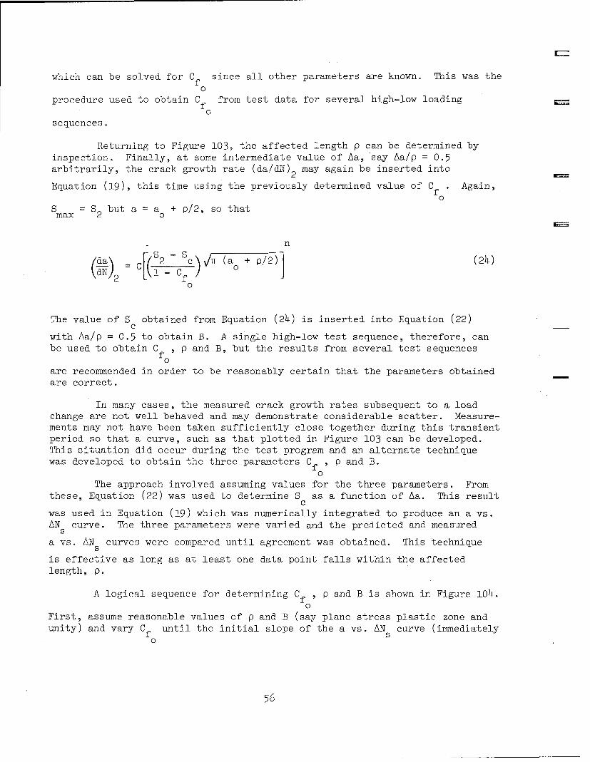
which can be solved for Cf since all other parameters are known. This was the

0procedure used to obtain Cf from test data for several high-low loading

0

sequences.

Returning to Figure 103, the affected length p can be determined by

inspection. Finally, at some intermediate value of Aa, say Aa/p = 0.5arbitrarily, the crack growth rate (da/dN)2 may again be inserted into

Equation (19), this time using the previously determined value of C f Again,0

S = S2 but a = a + p/2, so thatmax 2O

n

(/' C[('2 Cc) c (a + p/2)] (24)

0

The value of S obtained from Equation (24) is inserted into Equation (22)c

with Aa/p = 0.5 to obtain B. A single high-low test sequence, therefore, canbe used to obtain C , p and B, but the results from several test sequencesf

0

are recommended in order to be reasonably certain that the parameters obtainedare correct.

In many cases, the measured crack growth rates subsequent to a loadchange are not well behaved and may demonstrate considerable scatter. Measure-ments may not have been taken sufficiently close together during this transientperiod so that a curve, such as that plotted in Figure 103 can be developed.This situation did occur during the test program and an alternate techniquewas developed to obtain the three parameters Cf , p and B.

0The approach involved assuming values for the three parameters. From

these, Equation (22) was used to determine S as a function of Aa. This resultc

was used in Equation (19) which was numerically integrated to produce an a vs.AN curve. The three parameters were varied and the predicted and measured

s

a vs. AN curves were compared until agreement was obtained. This technique5

is effective as long as at least one data point falls within the affectedlength, p.

A logical sequence for determining Cf , p and B is shown in Figure 104.0

First, assume reasonable values of p and B (say plane stress plastic zone and

unity) and vary Cf until the initial slope of the a vs. AN curve (immediately0

56

following the load change) matches the data. Then the affected length, P, isaltered until the crack length when unretarded crack growth resumes agrees withthe data. As a rule, this crack length can be determined by plotting constantamplitude crack growth on the apparent steady-state growth for the data andestimating the point where the calculated and measured curves diverge as shownin Figure 104. Finally, the parameter B is varied until the number of delaycycles agrees with the data.

For the 2219-T851 aluminum alloy, the values of the parameters obtainedwere:

cf = o.4o 2

p P plane stress plastic zone radius

B ýý 1

It was shown in subsection 3.2.1 of this report that, for a differentanalytical technique, a plane strain plastic zone provided a good fit to thealuminum data. However, when using the assumed closure variation outlinedabove, it was found that the plane stress plastic zone provided the best fit.This is probably due to the manner in which the closure level is assumed tovary. When the closure stress approaches the stabilized closure level, thecrack growth rate is nearly constant amplitude and the resultant crack lengthvs cycles curve is almost the same as its constant amplitude counterpart. In

this case, the bulk of the retarded crack growth occurs over the first portion

of the affected crack length which, for the cases shown, approximates the

plane strain plastic zone.

Figures 105 through 107 present a vs. AN test data and predictionss

for several cases. The results verify that the parameters obtained reasonablyrepresent the material.

The Ti 6AI-4V titanium test data were considerably more difficult toanalyze. As discussed in Section 3 of this report, the only significant,

measureable parameter was the number of delay cycles, N . It was therefore

assumed that the values of Cf , p and B were identical to those for aluminum0

(p = plane stress plastic zone). Figures 108 through 110 show a vs AN data

and predictions for several titanium test specimens. The results again indi-cate that the parameters are reasonably representative of the data.

For materials such as the titanium investigated here, and others having

fairly high yield strengths, the affected lengths are generally quite small.It is necessary to obtain very accurate a vs N data subsequent to the load

change. However, if a sufficient number of less-accurately measured cases are

57

available, representing different stress intensities at the overload obtainedfor different stress combinations and crack lengths, it is possible to obtainreasonable values of Cf , p and B through a process of trial and error.

0Initially it was specified that the stress ratios for the two stresses

in the high-low sequence be zero. The procedure described above may be appliedto cases where R > 0 except that, to simplify the analysis, the minimum stressshould be the same for both maximum stresses. This requirement will becomeclear in the discussion regarding the effect of minimum stress variations onclosure level. In addition, the minimum stresses should in no case exceed,and preferably be much lower than, the closure stress expected for eitherthe high or low stresses in the sequence. If the closure stress is less thanthe applied minimum stress, Smin' then, no interaction should occur. There is

some disagreement as to whether this premise is correct or not (eg. Ref. 17),

but it has been assumed to be true here.

Effect of Minimum Stress on Closure - Tests have shown that the twoloading sequences shown in Figure 111 produce the same crack life subsequentto the load change. This result is shown schematically in the lower portionof the figure. Tests of this type were not run during this program. However,an indirect proof follows. It has already been shown that closure is a func-tion of stress ratio (ref. Equation 21) and, therefore, the stabilized valuefor the high stress in sequence B must be higher than the equivalent value insequence A. The explanation for similar crack growth behavior subsequent tothe load change is that the closure stress in sequence B quickly changes toapproximately the same value as in sequence A. The key parameter in thissudden fluctuation is the minimum stress.

Figure 112 shows actual crack closure (load vs. COD) curves for analuminum specimen subjected to an initial stress ratio of 0.5 and subsequentlyto a stress ratio o0 0.05. Because the maximum and minimum applied loads areknown and the ordinate is linear, any value of load on the curves may beobtained. Further, the displacements need not be calibrated since they areproportional to the local displacements near the crack tip and, as such, anynon-linearities on the load-displacement curve represent equivalent crack tipdisplacement non-linearities. The arrows parallel to the upper portion of thecurves indicate the loading phase (loading up or unloading) and the arrowsapproximately normal to the traces represent the estimated crack closure (andopening) levels. In all cases, the maximum applied load was the same (6 ksi).Apparent differences in maximum load and load ranges were caused by adjustingthe plotter controls.

During cycles 0 and 1, the closure stress is stable and slightlyhigher than the minimum stress. During the unloading portion of cycle 2, theclosure level remains the same. Loading up from the new minimum stress(R = .05), the crack opening stress is seen to be significantly lower than itspreceding closure value. After an additional cycle, the level is again reducedand by cycle 4 has apparently stabilized at a value of about 1.2 ksi (20% ofthe 6 ksi maximum). Although this value (20%) is somewhat lower than for

58

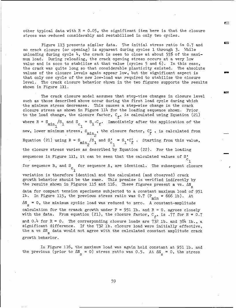
other typical data with R = 0.05, the significant item here is that the closurestress was reduced considerably and restabilized in only two cycles.

Figure 113 presents similar data. The initial stress ratio is 0.7 andno crack closure (or opening) is apparent during cycles 1 through 3. Whileunloading during cycle 4, the crack is seen to close at about 55% of the maxi-mum load. During reloading, the crack opening stress occurs at a very lowvalue and is seen to stabilize at that value (cycles 5 and 6). In this case,the crack was quite long so that considerable plasticity existed. The absolutevalues of the clousre levels again appear low, but the significant aspect isthat only one cycle of the new low-load was required to stabilize the closurelevel. The crack closure behavior shown in the two figures supports the resultsshown in Figure 111.

The crack closure model assumes that step-wise changes in closure levelsuch as those described above occur during the first load cycle during whichthe minimum stress decreases. This causes a step-wise change in the crackclosure stress as shown in Figure 114 for the loading sequence shown. Priorto the load change, the closure factor, CfV is calculated using Equation (21)

where R = S /S and S S .Cf. Immediately after the application of themin21 1 c1 1 f

new, lower minimum stress, S the closure factor, C, is calculated from

Equation (21) using R = S mn/S and S'c = SI'C' Starting from this value,mnan 2 1 c1 f

the closure stress varies as described by Equation (22). For the loading

sequences in Figure 111, it can be seen that the calculated values of S'c

1

for sequence B, and S for sequence A, are identical. The subsequent closure

variation is therefore identical and the calculated (and observed) crackgrowth behavior should be the same. This premise is verified indirectly bythe results shown in Figures 115 and 116. These figures present a vs. AN

5

data for compact tension specimens subjected to a constant maximum load of 951lb. In Figure 115, the previous stress ratio was 0.7 (Pin = 666 lb). AtAN = 0, the minimum cyclic load was reduced to zero. A constant-amplitude

s

calculation for the craack growth under P = 951 lb. and R = 0. agrees closelywith the data. From equation (21), the closure factor, Cf, is .77 for R = 0.7

and 0.4 for R = 0. The corresponding closure loads are 732 lb. and 384 lb., asignificant difference. If the 732 lb. closure load were initially effective,the a vs AN data would not agree with the calculated constant amplitude cracks

growth behavior.

In Figure 116, the maximum load was again held constant at 951 lb. andthe previous (prior to AN = 0) stress ratio was 0.5. At AN = 0, the stress

5 5

59

ratio was reduced to 0.3. The corresponding closure loads are 578 lb. and472 lb. Again, the previous high closure load did not affect the crack growthfor R = 0.3, since the calculated constant amplitude growth agrees closelywith the data.

The crack closure model performs this minimum-stress adjustment regard-less of the relationship between S and S2 (i.e., even for the case where

S2 S.*) The only criterion is the relationship between the minimum stresses.

Because of the manner in which the minimum-stress adjustment is per-formed, a single cycle of reduced minimum stress has the effect of immediatelyreducing the closure level, and affecting the subsequent crack growth. Thisconcept is easily extended to handle compression spikes and will be discussedsubsequently. It will be shown later that for certain materials, the impact

of this reduction is not very significant.

Effect of Single and Multiple Overloads on Subsequent Crack Growth -It has been shown by several investigators (References 14 and 18) that a singleoverload cycle, superposed on constant amplitude cyclic loading, produces alesser degree of subsequent retardation than several overload cycles. Noneof the currently existing models (References 10 and 11) differentiates betweenthe number of overload cycles. They assume that the crack growth subsequentto any number of overloads is always fully retarded. A method to account forthe number of overloads effect has been developed for the crack closure model.

In general, one overload cycle produces some subsequent retardation,

two overload cycles produce more, and so on. There appears to be a limit tothe amount of retardation which can be attained for a given material(References 4, 14 and 16). Figure 117 shows schematically how the closurestress might vary during a low-high loading sequence. Prior to the load change,the closure stress is that stabilized value, S associated with the initial

loading, SI. Subsequent to the load change to S2, the closure stress increases

to the stabilized value, S c2 associated with stress level S 2 Data gathered

02prior to and during this program indicates that the closure level varies as afunction of the number of cycles, NOL, of the overload stress level, S The

number of overload cycles at which no further increase in closure level occursis defined as N sat. If no overloads are applied, the closure stress does not

change and crack growth during subsequent cycling at Sl would be unretarded.

If N0L > N sat, the retardation of the crack growth during subsequent cycling

at S would be maximized. Intermediate values of N0L (0 < NL < N sat) would

produce intermediate values of retardation. Figure 118 presents this effectschematically.

6o

Some of the data gathered during this program indicated that the over-load ratio, O/L, must attain some minimum value before the overload stresshas any apparent effect on subsequent crack growth. (The overload ratio, O/L,was defined earlier as the ratio of the overload stress to the baseline stress,SoL/S.) For example, Figures 119 through 123 present a vsN data for specimens

subjected to single discrete overloads where the overload ratio was 1.25, 1.4and 1.5. Calculated constant amplitude growth curves (neglecting any growthor retardation due to the overloads) are also shown. It can be seen that thecalculated curves agree very closely with the data. This indicates that over-loads with O/L values <_1.5 have negligible effect on the crack growth behavior.Therefore, the closure stress is unaffected for 1.0 < O/L < 1.5.

Figure 124 presents the ratio, R (the calculated closure stress after

one overload cycle over the initial closure stress), vs the overload factor,OIL, for data gathered during several single overload events. The closurestress immediately after the overload, S , was calculated by assuming

c1

different values of S and comparing predicted a vs AN curves with the data.c1 s .

Equation (21) with the values of C o p and B for aluminum was used to definef0

the variation of S and Equation (19) was numerically integrated to obtain ac

vs AN . The values in parentheses represent the number of events analyzed tos

produce the plotted value. The diagonal, dashed line represents the case wherethe closure stress equals the stabilized value. If the calculated points fellalong this line it would mean that there is no difference between one and manyoverloads. It can be seen, however, that almost all of the values lie belowthe line. It can also be seen that R is equal to 1 up to an overload ratio

C

of approximately 1.5. This means that after one overload cycle, for O/L.. -1.5,the closure stress does not increase.

At O/L = 1.8, there is considerable scatter in the calculated results(1.2 < R < 1.8). These points were re-plotted in Figure 125 along with cal-c

culated values of Rc for values of NOL > 1. (Other data points for NOL = 50

to 2000 cycles produced values of R = 1.8 but are not shown here.) TheC

number of overload cycles that causes saturation, Nt, is apparently between

10 and 20. The trend of the data based on NOL > 1 indicates that the value

of Rc at NOL = I should be about 1.4. Since it was desired to produce a con-

servative prediction based on these data, a value of 1.2 was selected. Thismeans that the closure stress after NOL = 1 is 2/3 (1.2/1.8) of the stabilized

value and is conservative since the calculated closure stress is less than theactual closure stress. The calculated subsequent retardation will thereforebe less than the actual retardation.

61

The parameter y is defined as:

Closure stress after NOL (25)

Closure stress after Nsat

and is a function of the number of overload cycles, N OL For NOL 1, y = 2/3

and for NoL Nsat, y = 1. It was assumed, therefore, that the closure stressafter NOL = 1 was 2/3 of the stabilized closure stress regardless of the over-

load ratio. This assumption is shown as the solid line in Figure 124. Thedashed line represents the closure levels for N OL_ N sat. In no case, however,

can R be less than unity since the closure stress would not be expected toc

decrease after an overload(s) has been applied.

The data of Figure 124 are replotted in Figure 126 as y vs NOL for all

values where O/L 1.5. The value of y was assumed to vary linearly as:

N0L - 1 (26)

N sat

For 2219-T851 aluminum:

N -1

Yl = 2/3 so that: y = 2/3 + 1/3(Nt L 1 (2 6 a)

The value of Nsat was selected (somewhat arbitrarily) as 13, but is substan-

tiated by the results of Ref. 18. There, the authors indicated that for 7075-T6 aluminum, when NOL = 10, the delay (retardation) was nearly maximized. In

all probability, the expression used here for y as a linear function of NOL is

incorrect (and unnatural). It is suspected that y should approach a value of1 asymptotically. An insufficient number of values of NOL were investigated

to test this assumption and the crack closure model assumes the linear functionto be correct.

Titanium specimens subjected to single overloads with overload ratios of 1.25,1.5 and 1.8 were tested. Where the overload ratio was 1.25, the overload hadlittle or no effect on subsequent crack growth. Unlike the aluminum, thetitanium overload ratios of 1.5 did produce measurable crack growth retardation.

62

Results similar to the aluminum results were obtained although considerablescatter in the calculated values of y was encountered. These results arepresented in Figure 127. For the titanium, the parameters selected were:

Y = .8o

N =100.s at

This value for Nsat is supported by Wei (Ref. 14) who measured delay cycles

as a function of the number of applied overloads for Ti 6A1-4V titanium. He __

found that the number of delay cycles was maximized after approximately 100overload cycles under constant stress intensity conditions.

It is worth noting that the evaluation of y is based on data obtainedpredominately at stress ratios which were nominally zero. It is probablethat the variation of closure load with the number of overloads is signi-ficantly different at higher values of R. This conclusion can be reached byconsidering probable causes of the variation in closure with the number ofoverloads and some of the data presented in this-program.

Previous investigators (Ref. 19, for example) have attributed thevariation in retardation to the fact that, with increasing numbers of over-loads, the crack propagates further into the overload plastic zone beforethe return to constant amplitude loading. That this is not the governingphenomenon is demonstrated by the low values of Nsat found in this program

(particularly in aluminum), during the application of which a crack wouldpropagate through a very small percentage of the plastic zone. Additionally,the titanium, which has a much smaller plastic zone than the aluminum, requireda much larger number of cycles to reach saturation even though the overall rangeof crack growth rates investigated was nominally the same.

The number of cycles required for saturation is of the same order ofmagnitude as the number of cycles required to reach stability in a cyclicstress-strain test. This is what one might expect if saturation was reachedafter the local crack-tip residual stress pattern stabilized in a similarmanner. If this is indeed the governing phenomenon (and certainly local cyclicstress-strain behavior should play some role), then a significant variationin saturation cycles with stress ratio is to be expected. Consider a testbeing run at a high R value such that the closure load caused by an overloadis below the minimum baseline load. Subsequent cycling would produce totallylinear load-displacement records, the local stress-strain behavior would beessentially elastic, and no further changes in residual stress patterns wouldoccur. Therefore, at high R values, the number of cycles to saturation wouldbe one. The important point in this argument is that the closure load isbelow the minimum applied load. Thus, the amount of "crushing" or closing

63

below the closure level may control the number of cycles it takes to achievestability in the residual stress pattern and, therefore, to reach closuresaturation. A measure of the "crushing" might be the difference between Cf

and R as shown schematically in Figure 128.

The data of subsection 3.5 tends to support this conclusion. Considerfor example Figure 76. Retardation is obviously present. However, the modelpresently proposed predicts a closure level of 832 lbs. due to the basic con-stant amplitude loading and a closure load of 762 lbs. due to the single over-load application. Therefore, the model would predict no retardation. The lowclosure load is due to the fact that, after the first cycle, only 2/3 of theoverload saturation closure level is reached. At the other extreme, assumethat the saturation level is reached for this R value (1/3 for the overload)so that a closure load of 1069 lbs. is obtained. Then significant retardationwould be predicted. A more reasonable assumption might be a linear variationin y with (Cf - R). This would produce a closure load of 912 lbs.

Presently, there is insufficient data to determine whether or notthese hypotheses concerning the variation of the saturation behavior withstress ratio are valid.

Effect of Compression Loading on Closure - In the preceding discussion,it was shown that a single cycle of reduced minimum stress is treated as pro-ducing an immediate reduction in the closure stress. This concept can beextended to the case where the minimum stress is negative (compression).Figure 101 shows that, as the stress ratio is reduced below zero, the closurefactor decreases slowly. This implies that for both 2219-T851 aluminum, andTi 6A1-4V titanium, the application of compression stresses is only slightlymore damaging than the application of minimum stresses which are equal to zero.This is also apparent from the constant amplitude data, where the crack growthrate for R = -1 is only 33% faster than for R = 0 at a given AK (Equations laanrd 2).

The crack closure model treats the cases of negative (compression)loads as an extension of the minimum stress adjustment. Figure 129 showsschematically how the closure stress varies for the case of a high-low loadingsequence where the minimum stress of the low portion of the sequence, S ,min2

is negative (compression). Before the load change, the closure stress, S ,

is the stabilized value associated with the initial (high) stresses, S and

S . . Immediately after the load change, a new closure stress, S' = S Cmin1 c 1 1 f'

is calculated. Equation (21) is used to determine Cf and R is taken as

Smin2/S . The closure stress, Sc, then varies from S' to S as described bymn2 1 c c1 2

Equation (22).

64

Effect of Compression Spikes on Subsequent Crack Growth - Compressionspikes and underloads are treated by the model in the same manner as constantamplitude and step-wise loadings. Underloads are defined as single cycleexcursions of the minimum stress to lower tensile values, where the nominalstress ratio is greater than zero. These loading sequences are shown sche-matically in Figures 130 and 131. Prior to the application of the spike load,the closure level is the stabilized value, S , associated with the applied

cstresses S and S min. Immediately after the application of the spike loads,

a new, lower closure stress, S', is calculated from Equation (21) usingc

R = S 2/S . The closure level then returns to the stabilized level S in the

same manner as described under the heading "Increasing and Decreasing ClosureLevel" below.

For load sequences such as those described, and particularly duringspectrum loading, it is common to calculate modified stress ratios based onpreceding maximum stresses and current minimum stresses which are much lessthan -1. Actual values of R < -1 might also be encountered. Data were notobtained for R <-1 under constant amplitude loading conditions. Thereforethe closure behavior, either measured or calculated from crack growth ratedata for large negative R values, is unknown. Based on the behavior of Cf

in Figure 101, it appears that the closure level asympototically approaches

some minimum value as R becomes more negative. The model therefore treatsvalues of R < -1 as R = -1 until additional data for R < -1 is obtained.

Increasing and Decreasing Closure Level - It is necessary to definewhether the closure level is increasing or decreasing during variable amplitudeloading. The current closure stress is that value which exists prior to aload change. It may be modified by overload or minimum stress considerationsimmediately after the application of the new loadings. The expected closurestress is the stabilized value associated with the new loading.

If the current closure stress is greater than the expected value, adecreasing closure situation exists and the behavior of the closure stress isdefined by Equation (22). Generally, for this condition, the drop in closurelevel requires many applications of the new loading to propagate the crackthrough the affected length established by the previous loading. Conversely,when the closure level is increasing (current closure stress is less than theexpected closure stress), Equation (26) applies, and it takes very few cyclesof the new loading to regain a stabilized closure value. In the latter case,about 13 cycles are required for the 2219-T851 aluminum and approximately 100cycles for the Ti 6AI-4V titanium to attain stability.

Variable Amplitude Loading - Previous discussions have described howthe model treats crack closure during constant amplitude and discrete loadchange sequences. During variable amplitude loading sequences, load changesoccur much too frequently for stabilized conditions to occur between the loadchanges. Typically, several (or many) transient conditions overlap. Thefollowing discussion describes how the model treats these conditions.

65

Figure 132a presents schematically how the closure level varies forthe case of increased maximum load when the minimum load is held constant.Prior to the load change, S is stabilized at Sc . After the first cycle ofc c

S 2, Sc is Sc y from Equation (26). In this case, S y > Sc . Thereafter,

S increases to S by Equation (26). The number of cycles of S 2 required to

reach S is Nsat'c 2 sa

Figure 132b shows a similar case, except that immediately after theload change, Se2 y is less than S c In this case, the value of NOL in

Equation (26) is replaced by the value N' and y is replaced by S ISCL c 1c2

S C 1 N, L 1 (2 6 c)

S c 2 1+(- ' Nsat 1 )

The value of N' obtained from Equation (2 6 c) is the apparent number of over-OL

load cycles (cycles of S2 in this case) which have already been applied to the

crack. Cycles of S2 are then counted starting at NO' rather than zero, and

Equation (27) is used to calculate the closure behavior starting at N'L. It

can be seen that, for Sc > yS c, the number of overload cycles required to

reach Sc2 is always less than N sat. In the limit, when Sc1 S c2, the number

of overload cycles is zero and is physically consistent.

Figure 133 presents two variations of the cases previously discussed.In Figure 133a, the maximum stress is held constant while the minimum stressis increased. This case is handled in the same manner as those presented inFigure 132. The number of cycles to achieve stability is < N sat. In Figure

133b, the maximum and minimum stresses change as shown. Immediately after theload change, the minimum stress adjustment is employed to reduce the closurestress to S' Equation (26) is used to determine if a subsequent adjustmentc 2

upward to S" is required. If so, the closure stress then varies over Nc 2 sat

cycles to S (solid line). If not, the closure stress varies to S along

the dashed (alternative)line. In the latter case, NOL can be less than or

equal to N depending on the relative values of S' and S (alternative).sat

c2 2

66

The preceding discussion covered typical cases of increasing closure.All cases of increasing closure aretreated in the same manner. The extensionof these cases to variable amplitude loading is fairly simple and requiresonly the use of Equation (26c) to adjust the cycle count for use in Equation(26). In all cases, for S > S , or S > S' I, the closure condition is

.c2 . c1 c 2 c 2defined as increasing.

The treatment for decreasing closure is more complex for two reasons.First, many of the potential interaction situations were not investigatedduring the test program. Even those cases which were investigated were diffi-cult to analyze directly because of the limited amount of crack growth duringa given load level and because of the small affected lengths. For example, -KMit is difficult to apply several load sequences within a given affected cracklength (which may be of the order of 0.020 inch) and to optically measuretransient crack growth behavior during each of the load sequences to obtainmeaningful data. As described earlier, the crack growth subsequent to the loadchange was not well behaved, even for cases of discrete load changes. Secondly,from a modeling standpoint, a complex load history requires a complex book-keeping capability. The question of the significance of some previous loadsequence also arises. For these reasons, only those parameters deemed to havethe greatest influence on crack growth retardation are tracked by the model.These are:

p - affected cracklength over which transient behavior occurs

a - current crack length

a - crack length at which p was generated0

a - a + p, elastic-plastic interfacep o

a - crack length at start of current loadings

Smin - previous, smallest minimum stress which was applied whilep a <a<a

o p

S - current maximum stress

Smi - carrent minimum stress

S - existing closure stress

S - expected stabilized closure stress for S and Sc 2 min

67

The affected length, p, shown in Figure 134, is generated by someprevious maximum load, Sp, applied at a and assumed to be proportional to the

Irwin plastic zone radius:

P= o (27)

where a is the material yield stress. The coefficient 3 is assumed to be ay

variable and can be the plane strain value (,the plane stress value

or any other value which was determined to fit the data as described

previously. As long as the crack tip, a, is within the affected length(a < a < a ), transient conditions exist. For a less than a (not possible)

or greater than a , stabilized steady-state conditions exist. If, during the

application of a given load level, a equals or exceeds ap, stabilized conditions

prevail throughout the balance of that level. The extent of the elastic-plastic interface, a p, is updated (using S in Equation (27)) at the beginnning

and at the end .of each load level as required. Whenever a is updated, S isP Pset equal to S. For the following discussion, it is assumed that the cracktip is always within the affected length.

The crack length at the start of the current loading, a, is used in

Equation (22) to define the downward movement of the closure level. Thepertinent geometry is shown in Figure (134) and Equation (22) becomes:

Ba -a

S = S - S- (S -c 2 ) (a a ) (22a)

The previous, least minimum stress, Smin , is tracked for use in the

pminimum stress adjustment. Whenever a new minimum stress, Smin which is

lower than S . , is encountered, the minimum stress adjustment is applied to

pcalculate a modified value of Scl The effective stress is Smin/Sp for use in

Equation (23). In certain instances, the modified value of S exceeds thec8

68

original value of S c In this case, the original value of S is retained.

Finally, Smi is set equal to Smin.

p

The expected stabilized closure stress, Sc . is the endpoint closureC2

stress in Equation (22) or (22a) when a > a .p

Figure 135 presents schematically the treatment of three potentialsituations for a three level descending load sequence. The minimum stress istaken as zero for all load levels. In Figure 135a, there are a sufficientnumber of cycles of S2 and S3 to propagate the crack through the affected

lengths p1 and p 2 respectively. The subscripts of p are associated with thestresses which created each p (i.e. p1 was caused by S ). The appropriate

parameters are inserted into Equation (22a) and the closure behavior withineach affected length is defined. (The exponent B in Equations (22) and (22a)has been depicted as unity in all figures for convenience.)

Figure 135b shows the next higher level of complexity which can occur.

Here, an insufficient number of cycles of S are applied to grow the crack2

through a . The closure level has declined to a value S' where (S >P1 c 2 c 1

S ' > S ). In addition a < a so Equation (22a), for the closure vari-2 2 p1 -

ation during S3' becomes:

B

S = S S' -S for a < a < ac2 c2 Pls

Figure 135c presents a similar case except that a > a . NowP2 p.1

Equation (22a) becomes:

B

- - -- for a < aS C' S Sc a asPc2 c2 P3) s3) p 2

69

to define the closure variation during the application of S . The location

of a 0 , originally equal to a ,is now advanced to be equal to as3 or the crack

length from which the new elastic-plastic interface is measured. In addition,the value of S originally equal to S is updated to S2.

In all three figures, when the loading S3 is completed, steady-state

conditions exist and every parameter would be updated based on S . The

extension of these rules for more complex loadings follows logically.

Figure 136 presents cases where the maximum and/or the minimum stressesvary. In the first case, (Figure 13 6 a), the maximum stress is held c6nstantand the minimum stress decreases in steps. For this type of load sequence,only the minimum stress adjustment is employed at each load change to calculatea step-wise change in the closure level. Interestingly, this type of loadingsequence has no interactions and the crack growth during each part is solelyconstant amplitude in nature.

Figure 136b presents two sequences, the first requiring a minimum stress

adjustment and the second a simple application of Equation (22a).

A slightly more complex situation is depicted in Figure 13 6 c. At thepcLnt where S2 begins, the minimum stress also changes to S min2 . First, the

minimum stress adjustment is applied to calculate S' In Equation (21), RcI

is set equal to Smin /S to obtain C' and S' SI C'. The closure levelS2 1 f c f

then varies through the affected length, p, caused by SI, to Sc2 by

Equation (22a).

4.1.3 Results and Discussion

The proof of any model lies in its ability to predict the crack growthbehavior of a specimen, or component, subjected to any arbitrary loadingsequence. This section presents results obtained by the crack closure modelfor a variety of loading conditions. Almost all of the specimens and/orloading sequences were selected at random in an effort to be as objective aspossible.

Constant Amplitude - Figures 137 through 143 compare constant amplitudepredictions obtained by the model with test data. These results, obtained forvarious stress ratios for both aluminum and titanium, were used to verify thatthe closure equation (Equation 21) reasonably represents the material behavior.Figures 137 through 139 are for aluminum specimens subjected to stress ratiosof .5, 0 and -1 respectively. The good correlation is typical of the aluminumbehavior.

70

Figures 140 through 142 present the results for titanium specimenssubjected to stress ratios of 0.5, 0.3 and 0.05 respectively. Here, the

results are a little scattered. This was attributed to the basic material

scatter as described in Subsection 3.1.2 of this report. These results all

fall well within the scatterband described there.

The results presented in Figure 143 are in poorer agreement. The

prediction and a calculation using Equation (3), for reference, began at a= 0.5 inch ( s 774,000 cycles). Equation (3) was fitted to this particulardata (the only R = -1 titanium test) and is shown relative to the data inFigure 15e. There, it can be seen that for low values of AK, the data pointsexhibit somewhat faster growth than that of Equation (3). Since this is thecrack length regime where most of the cycles are used, the slight over-prediction of total life is not unexpected. I

The deviation between the prediction and the calculation usingEquation (3) can be attributed to the fact that the closure equation, Equation21, did not fit the rate data particularly well. This is shown in Table 14.

For R = -1, Equation (3) produced a crack growth rate of 5.5 x 10-7 inch/cycleat AK = 15 ksi Iinch. The closure equation, combined with the effectivestress crack growth equation, Equation (19b), produced an equivalent value of

4.07 x 10-7 inch/cycle. This results in a predicted life which is about 35%greater than the life calculated from Equation 3.

These last results (Figure 143) indicate that either the data are incor-rect (and that additional negative stress ratio tests should have been run forthe titanium) or, more likely, that the closure equation is not general enoughto properly represent different material behaviors.

Single Discrete Overloads - Figures 144 through 153 present data andpredictions using the crack closure model for 2219-T851 aluminum and Ti 6A1-4Vtitanium. Results for overload ratios, O/L, of 1.25, 1.5 and 1.8 are shownfor both materials. For aluminum with values of O/L = 1.25 and 1.5 (Figures144 through 147), the model predictions are quite accurate. For an overloadratio of 1.8 the results are of mixed quality. In Figure 147, the predictedlife is approximately 84% of the test life but, in Figure 148, the predictedlife is only 60% of the test life. It should be noted that the predictions areconservative or only slightly unconservative for all of the cases shown.

The predictions obtained for titanium (Figures 149 through 153) areless accurate than those obtained for aluminum. For the lowest overload ratio(1.25), the predicted life is 12% greater than the actual life, as shown inFigure 149. Figures 150 and 151 present results for O/L = 1.5. For these twocases, the predicted lives are 17% less than and 25% greater than the testlives. At an overload ratio of 1.8, the model under-predicts the test livesconsistently. For example, the predicted life is only 51% of the test lifein Figure 152 and 47% of the test life in Figure 153.

71

For both materials, as the overload ratios increase, the ratio of thepredicted life relative to the test life decreases. These results imply thatthere is an overload ratio effect, or a relationship between the overload stress(and/or baseline stress) to the material yield stress, or both, which has notbeen accounted for.

The number of overload ratios investigated was, of necessity, restric-ted. Perhaps higher values than those investigated would have proved to bemore productive. At the same time, however, it was desired to gather crackgrowth rate data over specified rate ranges which restricted the magnitude ofthe overloads. Further, in the case of the aluminum, stable tear considerationsplaced an upper limit of 30 ksi liT on the maximum stress intensity causedby the overload. The investigation of higher overload ratios requires thatsmaller crack lengths be employed. In turn, the crack growth rates subsequentto overloads become very low. These result in long test times and, potentially,effective stress intensity ranges which are below the threshold for fatiguecrack growth. Most of these comments would also apply to stress level invest-igations. In light of the above, it is felt that the results obtained thusfar are acceptable, particularly since they are almost always conservative.

Single Periodic Overloads - The predictions obtained by the crackclosure model for this type of loading are generally less accurate than thosepreviously described. Figures 154 through 161 present test data and predictionsobtained by the model for both materials. It can be seen that for 2219-T851aluminum, except for the case shown in Figure 157, the model consistently over-predicts the test life. In some cases, the predicted life is many times thetest life. These results are tabulated in Table 15 where the predictions wereextended to larger values than those shown in the figures. Even so, forspecimens AD-25-26 and -29, the prediction was terminated to reduce runningtime on the computer.

The over-predicted results for the aluminum can be traced to the mannerin which the model treats overloads. Unless there are a sufficient number oflow loads to cause the crack to escape the effect of the overload, the closurelevel continues to increase. This effect is shown schematically in Figure 132.Each time the overload is applied, the closure stress increases. During theapplication of the low loads, the closure stress decreases to some extentdepending on how far the crack extends through the overload-affected length.If the closure stress has not decreased sufficiently when the overload isapplied again, it then increases by Equation (26c). If the closure stressdecreases enough, a quasi-stable situation develops where the closure stressoscillates about some average value. For the case of the aluminum, the cracklengths affected by the overload are quite large due to the relatively lowmaterial yield stress. If only a few cycles of low load are applied (as wasthe case here), the crack progresses only a small amount between overloads.Further, the aluminum has a value of Nsat equal to only 13 cycles. This means

that less than 13 occurrences of the overload causes the closure level to attaina value which is essentially the stabilized value associated with the overload.Of course, during the application of the low loads, the crack propagated partof the way through the overload-affected length and the average closure level

72

was somewhere between the stabilized values for the overload and the low loads.For the first five cases shown in Table 15, the combination of overload ratioand/or few low-load cycles caused the calculated closure level to hover around

a value which was close to the stabilized value for the overload. This resultedin a small effective stress range for the low-loads and a comensurate low crack

growth rate. In the last case (Specimen AD-25-27), the overload ratio was

low and the number of low-load cycles was sufficient to bring the averageclosure level into what is apparently the right range based on the goodprediction.

The titanium predictions (Figures 158 through 161) are better thanthose for the aluminum. For cases where the overload ratio is 1.25 (SpecimensTD-25-32, -39 and -31), the predictions are only slightly greater than thetest values. For cases where the overload ratio is 1.8, the predictions areshorter than the test lives. These results for titanium are consistent withthose discussed earlier for single discrete overloads. There, it was con-cluded that the effect of a single overload on subsequent crack growth, wherethe overload ratio was 1.8, was not strong enough. The closure level did notincrease enough to produce sufficient subsequent retardation. It is apparentthat the parameters for single overload applications in titanium have not beencorrectly defined.

Based on the aluminum results, it apppears that the model requiresadditional work for the single periodic overload cases. However, there werean insufficient number of different overload ratios and applications of lowloads to perform any meaningful effort.

Multiple Overloads - Multiple overloads fall into three basic cate-gories. First is the case of many overloads applied (NoL > N sat). Second

are situations where 1 < N0L < N sat. Finally, there are multiple periodic

overloads, which are essentially two-level block loading programs.

Several predictions using the crack closure model for situations whereNOL > Nsat were presented in Figures 105 through 107 for 2219-T851 aluminum

with overload ratios of 1.8, 1.6 and 1.5. Figures 108 through 110 presentedsimilar results for titanium with O/L = 1.25, 1.5, 1.6 and 1.67. To completethe range of overload ratios, Figures 162 and 163 present test data andpredictions using the crack closure model for 2219-T851 aluminum with O/L = 1.25and 1.5 respectively. Similar results are shown in Figure 164 for titaniumwith O/L = 1.8. For all of the cases, the predictions agree very closely withthe test data.

Figures 165 through 168 present similar data and predictions where theminimum load was maintained at a high level so that the stress ratio for thebase loading was 0.50. The minimum load during the application of the overloadsequences was maintained at the same level as the minimum load for the baseloading. These predictions, most of which fit the data quite well, indicatethat the model not only accounts for the retardation caused by the overloads,

73

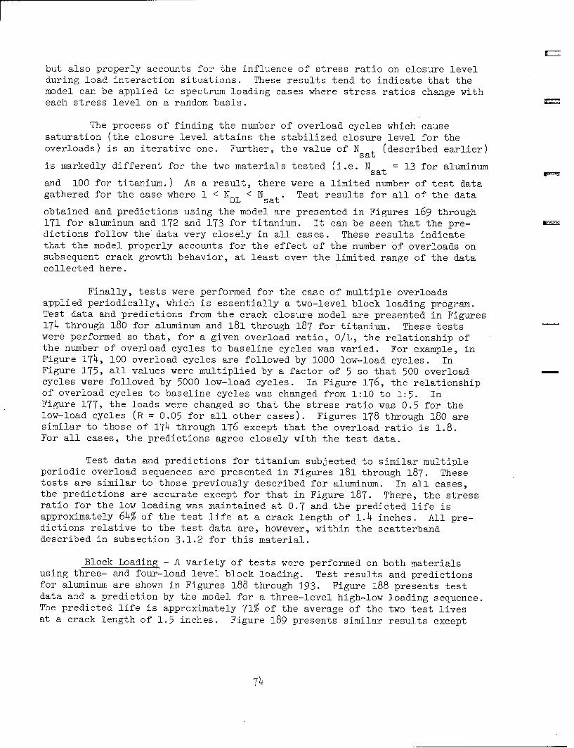
but also properly accounts for the influence of stress ratio on closure levelduring load interaction situations. These results tend to indicate that themodel can be applied to spectrum loading cases where stress ratios change witheach stress level on a random basis.

The process of finding the number of overload cycles which causesaturation (the closure level attains the stabilized closure level for theoverloads) is an iterative one. Further, the value of Nsat (described earlier)

is markedly different for the two materials tested (i.e. Nsat = 13 for aluminum

and 100 for titanium.) As a result, there were a limited number of test datagathered for the case where 1 < NOL < N sat. Test results for all of the data

obtained and predictions using the model are presented in Figures 169 through171 for aluminum and 172 and 173 for titanium. It can be seen that the pre-dictions follow the data very closely in all cases. These results indicatethat the model properly accounts for the effect of the number of overloads onsubsequent crack growth behavior, at least over the limited range of the datacollected here.

Finally, tests were performed for the case of multiple overloadsapplied periodically, which is essentially a two-level block loading program.Test data and predictions from the crack closure model are presented in Figures174 through 180 for aluminum and 181 through 187 for titanium. These testswere performed so that, for a given overload ratio, O/L, the relationship ofthe number of overload cycles to baseline cycles was varied. For example, inFigure 174, 100 overload cycles are followed by 1000 low-load cycles. InFigure 175, all values were multiplied by a factor of 5 so that 500 overloadcycles were followed by 5000 low-load cycles. In Figure 176, the relationshipof overload cycles to baseline cycles was changed from 1:10 to 1:5. InFigure 177, the loads were changed so that the stress ratio was 0.5 for thelow-load cycles (R = 0.05 for all other cases). Figures 178 through 180 aresimilar to those of 174 through 176 except that the overload ratio is 1.8.For all cases, the predictions agree closely with the test data.

Test data and predictions for titanium subjected to similar multipleperiodic overload sequences are presented in Figures 181 through 187. Thesetests are similar to those previously described for aluminum. In all cases,the predictions are accurate except for that in Figure 187. There, the stressratio for the low loading was maintained at 0.7 and the predicted life isapproximately 64% of the test life at a crack length of 1.4 inches. All pre-dictions relative to the test data are, however, within the scatterbanddescribed in subsection 3.1.2 for this material.

Block Loading - A variety of tests were performed on both materialsusing three- and four-load level block loading. Test results and predictionsfor aluminum are shown in Figures 188 through 193. Figure 188 presents testdata and a prediction by the model for a three-level high-low loading sequence.The predicted life is approximately 71% of the average of the two test livesat a crack length of 1.5 inches. Figure 189 presents similar results except

74

that the loading sequence is. reversed to low-to-high. Again, the predictedlife is about 71% of the test life at a value of a = 1.5 inches.

Block random loading was applied to the specimens shown in Figure 190.There, the load levels were maintained at the same values as for the low-highand high-low sequences. In those cases, a total of 6000 cycles was appliedin each block.

For the randomized loading, each level was reduced by a factor of tento a total of 600 cycles per block, for convenience in testing. These cycles =were randomly ordered within the block, but each block was identical. In thiscase, the predicted life is about 53% greater than the average of the testlives at a crack length of 1.5 inches.

Figure 191 presents data and predictions for specimens subjected tolow-high and high-low sequences, where the minimum load was maintained 500 lb.There, the stress ratio for the lowest load was 0.50 as compared to 0.05 forthe previous cases. In addition, the load was reduced to zero at randomintervals. This reduction is similar to a ground-air-ground loading cycle.The predictions neglect this zero load application and are based solely on theload values shown in the table in Figure 191. This was done as a conveniencein making the predictions. However, it will be shown that the introduction ofan occassional underload spike (or compression spike) has very little effecton specimen life. On this basis, the predictions which agree closely withthe data are considered to be valid.

Figure 192 presents results for specimens subjected to the randomizedspectrum. The single prediction nominally describes the average of the crackgrowth behavior for both specimens.

The results for the only four-level block loading test performed onaluminum are presented in Figure 193. The loads were identical to the valuesgiven in Figure 189 except that a single cycle of 1000 to 25 lb. was added toeach block. The crack closure model predicts a life which is approximately67% of the test life at a = 1.5 inches. At that crack length, the test lifeis 52 blocks which is identical to the life of Specimen AG-25-08 (Figure 189),where the initial crack length is nearly the same. The single cycle of 1000lb. had negligible effect on the crack growth of Specimen AG-25-25 (Figure193). The model predicts essentially the same result: 67% vs 71% of the testlife at a = 1.5 inches.

The predictions obtained for titanium, using the model, are typicallyless accurate than those obtained for aluminum under nominally similar condi-tions. Figures 194 and 195 present data and predictions for specimens sub-jected to a three-level low-to-high block. The predictions are quite poor,yielding lives of 16% and 48% of the test values respectively. In Figure 196,a prediction is presented which is 51% of the average life for the two testspecimens shown. There, the loading sequence was high-to-low. The low pre-dictions in all three cases can be traced to the affected crack lengths causedby the higher loads. It is apparent that these values are too low, and that an

75

increase in their magnitudes would cause the average crack growth rates todecrease. Figure 197 presents a prediction and test values for specimenssubjected to essentially the same loads as those in Figures 195 and 196. Thedifferences are that the minimum load was not held constant in this case butwas 10% of the maximum load in each level, and that the loads were appliedin a randomized sequence, 600 total cycles to the block. There, the predic-tion is fairly good. In Figures 198 and 199, the load ranges were held con-stant, but the minimum load was increased to 400 lb. so that the stress ratiofor the lowest loading was one-third. The loads were applied in ascendingand descending order. The predictions are reasonably close to the data.

Figure 200 presents results for four-level block loading tests andpredictions. Again, the model predicts short lives which are 42% and 55% ofthe test values for the high-low and low-high sequences respectively.

Typical Aircraft Spectra - Tests were performed on panel specimens torepresent typical aircraft spectrum loading. The test results and predictionsare presented in Figures 201 for aluminum and 202 for titanium. In this case,two predictions were made. The first neglected levels 63 and 64 of the spec-trum, the first of which is applied once every six blocks and the second, onceevery eighteen blocks. The second prediction included the application oflevels 63 and 64 once every block. The actual predicted life would lie some-where between the two predictions. For the aluminum, the average of the twopredictions is 58% greater than the test life at a half crack length of 0.7inch. Again, the titanium prediction is short, the average being 42% of thetest life at a half crack length of 0.9 inch.

Compression and Underload Spike Loads - One difficulty with currently-available models is that they do not accept compressive loads or stresses.Even for the case where the stress ratio for the base loading is greater thanzero and a tensile overload is followed by a zero load (underload), thesemodels neglect the underloads. The crack closure model accounts for thesesituations. However, all of the following examples are based on the crackclosure data obtained from single tests at R = -1 for both materials. Con-sidering this, the results obtained indicate that the concepts are basicallysound.

Figures 203 and 204 present data and predictions for 2219-T851 panelspecimens subjected to occassional compression spikes (single compression loadcycles). In the first figure, the base stress range was 0.3 to 6 ksi tension.Compression spikes ranging from 3 to 12 ksi were applied in a quasi-randommanner. The model overpredicts the test life by 20% at a half crack lengthof approximately 1.4 inches. It is interesting to note that a constant ampli-tude calculation for the base loading (6 ksi, R = .05) yields a life which isalmost identical to the prediction. A similar calculation for R = -1 is alsoshown and yields about 85% of the test life at the same half crack length. Theimplication of these results is that the compression spikes have very littleeffect on the overall life. This is substantiated by the results shown inFigure 204 where, in this case, the model under-predicts the test life byabout 18%. Although it is not shown, a constant amplitude calculation using

76

S = 10 ksi and R = .05 produces almost the same life as the prediction. Theprediction errors of +20% and -18% are within normal data scatter.

The negligible effect of the compression spikes are caused by twoseparate effects. First, for a fully-reversed loading where R = -1 (orapparently for even lower values of R), the closure stress of Figure 101 doesnot decrease very much. At the base loading with R = .05, the closure levelis about 41% of the maximum stress while, at R = -1, it is 34.7% of the maximumstress. In this case, the base closure stress is 4.1 ksi. After compressionspike, it is 3.47 ksi and has only decreased by 10%. For values of R between =-1 and zero, the difference is even smaller.

The second reason for the small effect of the compression spikes isthat it takes about 13 cycles of the base loading for the closure level toregain its original value. These few cycles are an extremely small part ofthe overall life of the specimen.

Figure 205 presents similar test results and a prediction for atitanium specimen subjected to similar loading. At a half crack length ofone inch, the model predicts a life which is 42% greater than the test life. Inthis case, it would appear that the compression spikes, ranging in value fromR = .5 to R = -2, have some effect on the subsequent crack growth. This effectwould be manifested in an increased crack growth rate subsequent to the appli-cation of a compression spike. However, Figure 206 indicates that this isnot the case. There, crack length is plotted against cycles since the com-pression stress, AN . Data and constant amplitude calculations for 10 ksi

5

and R = .05 are shown. It can be seen that the data do not generally exhibita faster crack growth rate than normal immediately after the compression spike,but do exhibit a general, overall crack growth rate which is slightly fasterthan the calculated behavior. For example, starting at a half crack lengthof 0.5 inch, the data and calculated crack length differ by about 0.030 inchafter 60,000 cycles. The average calculated crack growth rate is about 75%of the measured rate. These differences are cumulative, and account for mostof the error in the prediction shown in Figure 205.

Figure 207 presents data for an aluminum specimen subjected to occas-sional tensile overload spikes followed by compression spikes. For the firstthree events, the tensile spike overload ratio is 1.5. It was shown earlierthat, for aluminum, overloads of this magnitude have negligible effect on thesubsequent crack growth. For the 4th, 5th and 6th events, the overload ratiois 2.1 for the tensile spikes. Overloads of this magnitude are expected tohave a significant effect on subsequent crack growth rates. The data indicatesthat this is the case.

It is interesting to note that the compression spike did not reducethe retarding effect of the tensile overload for any of the nine events. Thiswas verified by making another prediction which neglected all of the com-pression spikes. The result was identical to the prediction including thosespikes. To understand the reason for this, follow the sequence of calculations

77

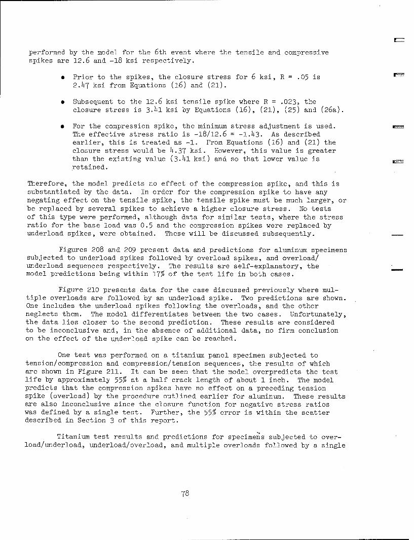
performed by the model for the 6th event where the tensile and compressivespikes are 12.6 and -18 ksi respectively.

"* Prior to the spikes, the closure stress for 6 ksi, R = .05 is2.47 ksi from Equations (16) and (21).

"* Subsequent to the 12.6 ksi tensile spike where R = .023, theclosure stress is 3.41 ksi by Equations (16), (21), (25) and (26a).

" For the compression spike, the minimum stress adjustment is used.The effective stress ratio is -18/12.6 = -1.43. As describedearlier, this is treated as -1. From Equations (16) and (21) theclosure stress would be 4.37 ksi. However, this value is greaterthan the existing value (3.41 ksi) and so that lower value isretained.

Therefore, the model predicts no effect of the compression spike, and this issubstantiated by the data. In order for the compression spike to have anynegating effect on the tensile spike, the tensile spike must be much larger, orbe replaced by several spikes to achieve a higher closure stress. No testsof this type were performed, although data for similar tests, where the stressratio for the base load was 0.5 and the compression spikes were replaced byunderload spikes, were obtained. These will be discussed subsequently.

Figures 208 and 209 present data and predictions for aluminum specimenssubjected to underload spikes followed by overload spikes, and overload/underload sequences respectively. The results are self-explanatory, themodel predictions being within 17% of the test life in both cases.

Figure 210 presents data for the case discussed previously where mul-tiple overloads are followed by an underload spike. Two predictions are shown.One includes the underload spikes following the overloads, and the otherneglects them. The model differentiates between the two cases. Unfortunately,the data lies closer to the second prediction. These results are consideredto be inconclusive and, in the absence of additional data, no firm conclusionon the effect of the underload spike can be reached.

One test was performed on a titanium panel specimen subjected totension/compression and compression/tension sequences, the results of whichare shown in Figure 211. It can be seen that the model overpredicts the testlife by approximately 55% at a half crack length of about 1 inch. The modelpredicts that the compression spikes have no effect on a preceding tensionspike (overload) by the procedure outlined earlier for aluminum. These resultsare also inconclusive since the closure function for negative stress ratioswas defined by a single test. Further, the 55% error is within the scatterdescribed in Section 3 of this report.

Titanium test results and predictions for specimens subjected to over-load/underload, underload/overload, and multiple overloads followed by a single

78

underload, are presented in Figures 212 through 214. Like the aluminumresults, the predictions agree closely with the data (greatest error 20 %)for all three cases.

Based on the results presented here, it is felt that the model accountsfor compression and tension/compression interactions fairly well. This makesit possible to account for, rather than disregard, excursions to zero load and/or load reversals for typical aircraft spectra. It should be noted also that,in general, the application of occassional compression or underload spikeshad little effect on the overall specimen life. Where they were preceded by a -single overload cycle, they had minimal influence on aluminum, but did tendto offset the overload effects on titanium. Where an underload spike was pre-ceded by multiple tensile overloads, it significantly reduced the retardingeffects of the overloads in both materials. _-

It is suspected that compressive spikes, following single tensileoverloads which are of sufficient magnitude, may negate at least partiallythe retarding effect of the overload. However, none of the specimens testedduring this program had high enough single overloads to test this theory.

4.1.4 Crack Closure Model Logic Diagram

Figures 215 and 216 present the overall and detailed logic flow forthe crack closure model. These charts are presented to provide additionalclarification of the decision processes of the model. Certain functions areused in the charts and are described below. The significant equations arereproduced here for convenience.

F(a) = Converts stress to stress intensity

da/dN(AK eff) = Crack growth rate based on AKeff, Equation (19)

Cf(R) = Cf as a function of R, Equation (21)

Sc(Aa) = function for decreasing closure, Equation (22)

y(J) = function for increasing closure, Equation (26)

p = governing affected crack length

da )A C[(Smax - S F n (19)

(7efff 1 1

C (R) = C + (C o C +R)p (21)

79

BS (Aa) (SSc - ) ; o Aa p (22)

y (j) = yI + (1 - Y)NOsa 1) (26)Nsat-

p(S (max)) - F(a) S(max) 2

The charts are self-explanatory and, coupled with the discussion in subsection4.1.2 of this report, should allow convenient use of the model.

4.1.5 Basic Data Requirements

The crack closure model offers a greater sophistication and variety ofloading options than currently available crack growth interaction mathematicalmodels. As a result, the basic data required to use the model are more complexthan for the other models. Additional data requirements center principallyaround the measurement of crack closure and the effects of number of overloads.

The crack closure model requires constant-amplitude crack growth ratedata for at least three stress ratios. Two of these should be R = -1 andzero. The third stress ratio must be greater than zero, but less thanthe stress ratio cutoff value. If a value greater than the cutoff is used, anerroneous crack closure function will result. Unfortunately, there is nomethod of determining the cutoff value other than by obtaining crack growthrate data at various positive stress ratios and then comparing the results ona rate vs stress intensity range basis. Numerical procedures can be an aidin this effort. For example, Equation (1) can be used in conjunction withleast squares and trial and error procedures to obtain q and R . Alterna-

cotively, the data can be plotted and the stress ratio cutoff value can bedetermined by inspection. The coefficient C and exponent n obtained fromEquation (1) are used in Equation (19) to calculate crack growth rates.

The constant amplitude data are used as described in subsection 4.1.2to obtain the closure Equation (21) as a function of the closure factors atR = 0 and -1, (C and C f). There the crack growth rate data were used in

Equation (19a) to relate closure factors at stress ratios other than zero tothe closure factor at R equal to zero. It should be noted that these dataonly relate the closure factors, and do not define their absolute values.

80

The magnitude of the closure factor at some stress ratio must bedetermined. A stress ratio of zero is suggested for convenience. However, aspointed out earlier, other values of stress ratio may be used with successexcept that R must be less than the cutoff value, R co to obtain a valid

result.

The closure factor at the stress ratio selected may be measured usingtechniques similar to those described in subsection 2.4 of this report. Itwas pointed out there that experimentally-obtained values, based on the results =of this program, generally exhibit considerable scatter. Comparatively smallvariations in the closure factor can produce large errors in predicted life,depending on the type of loading. As a result, an analytical method ofdetermining the closure factor is suggested.

One method, outlined in Subsection 4.1.2, was used with success inthis program. The technique employs Equation (22) and the numerical inte-gration of Equation (19). The use of this technique requires the results fromat least one test where the loading sequence is high-to-low. As described inSubsection 4.1.2, the method is iterative, but other useful data can beobtained. In addition to the closure factor, Cf , the affected crack length

0and the exponent B in Equation (22) can be obtained. Since these parametersare also required as input data, the proposed test serves a three-fold purpose.

Finally, data pertaining to the number of overloads must be obtained.As described in Subsection 4.1.2 (Effect of Single and Multiple Overloads onSubsequent Crack Growth), the crack closure model assumes that the closurestress varies linearly as a function of the number of overloads applied. Therequired input data are y and N sat, which were described in relation to

Equation (26). The parameter y is the effectiveness of a single overload

cycle on increased closure level, while Nsat is the number of overload cycles

required to achieve saturation.

These parameters are obtained from test results for different numbersof overload applications. Although the value of Nsat is generally unknown, the

results from this program and other sources indicate that Nsat is from 10 to

20 cycles for aluminum alloys, and is approximately 100 for titanium. The testsequences shown in Figures 172 and 173, with the numbers of overloads alteredto suit the material, provide a good range of values. The results from atleast one single overload test are required to obtain y1.

The analytical procedures used to obtain y and Nsat in this program

are outlined below:

1. Obtain test data (a vs cycles) for different values of N0L where

the minimum stresses for both the overloads and baseline loadingare zero or nearly zero.

81

2. Using the crack length vs cycles after the overload(s) and

3. The previously determined values of Cf 9 B and p,0

4. Let S c in Equation (22) be an unknown.

5. Numerically integrate Equation (19) using different values of K c

(or S c ) until the calculated crack length vs cycles curve fits

the data. Note that S C must be greater than S C in Equation (22).

6. Using the value of S obtained from a single discrete overloadc 1

case, determine y 1 from Equation (25), taking N OL ý 1. For the

case where the minimum stresses are all zero, the closure stressafter N sat is C f times the maximum overload stress.

0

7. The value of y must be greater than the reciprocal of the overload

ratio, O/L. As mentioned earlier, unless the overload ratio forsingle overload application exceeds some minimum value, the over-load has negligible effect on subsequent crack growth. The minimumvalues of O/L were found to be approximately 1.5 and 1.25 for2219-T851 aluminum and Ti 6Al-4V titanium respectively. If y 1is approximately equal to the reciprocal of O/L, the test resultsare questionable and a larger overload ratio should be used.

8. The value of N sat can be determined by plotting the ratio of S C i(or K C. ) from Step 5 above to the stabilized closure stress for

Ithe overload against the number of applied overloads. This methodis shown in Figures 126 and 127 where y equals the ratio of theclosure stress after N OL overloads to the stabilized closure stress

for the overloads. The value of N sat is the value of N OL for

Y = 1.

To summarize, the data required as input for the crack closure modelare:

a. Crack growth rate data at three stress ratios. These yield thecrack growth coefficient, C, and exponent, n.

b. Closure factor at R = zero, C f0

82

c. Closure factor at R = -1, Cf and exponent p (obtained from a.and b.).

d. Affected crack length, p, and exponent, B, for use in Equation (22).

e. Parameters y and Nsat for Equation (26).

4.2 RESIDUAL FORCE MODEL __

4.2.1 Concepts

The effective stress range approach seems to be the most straightfor-ward method of explaining crack growth interaction effects. For example, itwas shown in Ref. 5 that the Wheeler Model (Ref. 10) can be related to theEffective Stress Retardation Model (Ref. 11). The Effective Stress RetardationModel can, in turn, be related to our crack closure model. Since all of thesemodels can predict certain crack growth interaction effects, it was thoughtthat a model based on the distribution of residual stresses left in the wakeof a propagating crack could provide a basic understanding of the overallcrack growth phenomenon. As a result, the Residual Force Model was developed.Although some analytical problems related to certain crack growth interactioneffects were encountered, the basic concept is appealing since it may ulti-mately lead to a prediction model which is less empirical than those currentlyavailable. The development of the Residual Force Model and the resultsobtained using it are described below.

4.2.2 Application to Model

Elber (Ref. 15) proposed that the phenomenon of crack closure could beexplained by the existence of residual tensile strains left in the wake of apropagating crack. These deformations cause interference along the fracturesurface and, as the remotely applied stress, S, is reduced to zero, the crackcloses at some positive stress. The stress distribution caused by the crackface interference tends to prop the crack open. Figure 217a shows this conceptschematically. A crack of half length a. is subjected to a remote tensilestress, S, which causes a plastic zone of extent py. When the remote stress,

yS, is removed, a reverse plastic zone of extent, ry, remains defining an area

of compressive residual stresses. In Figure 217b, the crack has propagated toa new half length, a, and the crack tip is part way through the envelope ofcompressive residual stresses developed as the crack propagates. Figure 217cshows a residual stress distribution, S r, which represents the integrated valueof the residual forces existing from a rto a. Extending this concept to the

0

case where the crack has propagated a long distance, (Figure 217d), the crackis now subjected to the residual stress, S., along the entire length of its

83

faces. During the application of remote stress S, the crack tip stress

intensity is composed of two parts:

K = S 7a (28)

and

K r S r V/Tra (29)

For the case when S > S r5 the effective stress intensity is given by super-

position as:

AK eff = (S - S r (30)

If the crack can propagate only when it is open, as proposed by Elber, thenAK eff is the stress intensity range which should be employed to compute crack

growth.

In an effort to define the magnitude and extent of the residual stress,S r the following assumptions were made.

" S r is proportional to S and may be proportional to SIG y where a yis the material tensile yield stress.

" S r is related to the applied stress ratio, although no correlation

has been found.

" The extent of S r due to the application of one cycle of tensile

loading is one quarter of the maximum plastic zone size, assuggested by Rice (Ref. 20) and is given by

r K ) 2 (31)y 2a

where

for plane stress27T

and

for plane strain

84

Initially, it seemed that S should be equal to the material com-r

pression yield stress. However, a review of Equations (28) - (30) revealedthat the crack could only be opened by the application of S > a . ExperienceYindicates that this is not the case and that S must therefore be somethingrless than a . It was decided that, since the value of S was not known, it

y rwould be taken as:

S = cS (32)r

Further, initial analyses indicated that S should be proportional to ther

ratio of applied stress over the yield stress:

S =L S G (33)r (\ y

If the residual force proposition holds, then Equation (33) implies that allmaterials should show a stress level effect on crack growth rates, even duringconstant amplitude crack growth. Some materials strongly exhibit such aneffect, while many materials do not. Because our interaction studies usingthe Residual Force Model have to date been limited to 2024-T3 which is aninsensitive material, Equation (32) has been used.

An interesting effect produced by this model is that delayed retarda-tion is predicted. It was found that the delay period depends on the number ofoverloads applied and that as the number of overloads increases to the satur-ation value, the delay period decreases to zero. In addition, the modelpredicts acceleration when changing from a low load to a high load. Theseresults are included in the following discussion of the development of theworking model.

Figure 218a shows a crack which has propagated to a half length, a ,

under the influence of remote stress SI, which has caused the residual stress

S r to be developed. At half length a0, a remote stress S2 ( where S2 > S1)

has been applied and then removed. The plastic zone p caused by S2 is shown,along with the reverse plastic zone r which exists when S returns to zero.

y 2The crack then continues to propagate under the influence of SI.

85

Immediately after the application of S2 , and neglecting any growth

during the application of S 2 , the residual forces (stresses) acting behind

the crack are those caused only by the application of SI, and the residual

stress intensity is the same as for the constant-amplitude case for SI.

However, as the crack begins to propagate into the reverse plastic zone causedby S2 5 the residual forces Sr begins to act behind the crack tip, and an

2increase in K occurs. When the crack half length is, a + r , the influencer y

of S is most prominent and K is a maximum. As the crack continues tor2 r

propagate, S becomes remote from the crack tip so that its effect on K isr2 r

reduced, and when the crack half length is large relative to a + ry , the effect

of S on K approaches zero.r2 r

If a crack propagation law of the Paris type is used, so that:

da = C(AKff)n (34)

and AKeff = K - Kr (35)

then AKeff is smallest when the crack half length is a + ry and da/dN is the

smallest at the same point. Therefore, the minimum crack growth rate occursat a point ry, from where the overload was applied and delayed retardation has

been represented by the model. Figure 218b shows the resulting crack growthrate schematically.

To test this approach, an equation of the form

Kr=S sinl(c) sinl()- 1 _(L)2 +1 - ()2]

in = sin C nY-I +

was taken from Ref. 21. The force distribution for use in this expression isshown in Figure 219. The equation given in Ref. 21 has been multiplied by twoto account for forces acting on both surfaces of the crack. At any cracklength, a, it is a simple matter to sum the effects of the various residualstress distributions over the crack half length from zero to a, to obtain thetotal K

r

86

One drawback of this approach, is that it predicts that an overloadaffects the residual stress intensity even after the crack has propagatedseveral plastic zone sizes. Recent experimental investigations, includingRef. 4, indicate that this is not the case and that the effect of the overloadshould have been dissipated by the time the crack has propagated through adistance approximately equal to the plastic zone caused by the overload. Inan effort to circumvent this drawback, it was decided to include only theeffect of those residual stresses which extend back from the crack tip a dis-tance equal to the distance from the crack tip to the elastic-plastic inter-face. This approach forces the residual stress intensity to return to aconstant-amplitude value when the crack has propagated through one plasticzone. Although this assumption is open to question, some justification mightbe found in the fact that those forces closest to the crack tip have the mosteffect on crack tip behavior.

An equation for the effective stress intensity range, AKeff, was

finally formed as

AKeff= S - - - sin-b)-- 1 (- ) +1 _ ]

(36)

In order to relate AK to the applied AK, it is necessary to introduce aeff

modifying factor of the form

r sin- i(a (a - py (36a)7 2

as a denominator in the crack growth equation such that

"daN C/(AK e

n

C

{' - sin-1 a - - b

a 7(37)

87

For the constant amplitude case, this equation reduces to:

n

Tr -- sin +___ 1- ___ (38)-17 ( a_ (a a~)

- = C

sinT (a - a - Pyj

or

S a csr

Obviously, these expressions do not account for stress ratio or stresslevel effects. However, it is felt that when an expression relating S rto

stress ratio and/or level is developed, it could be incorporated as a simplemodification.

4.2.3 Results and Discussion

The model was tested using data which strongly exhibited delayed retar-dation. As stated earlier, this phenomenon was not strongly evident for thematerials tested during this program. Therefore, data from the literaturewere employed.

Figure 220 shows data for 2024-T3 aluminum taken from Ref. 4 forseveral loading sequences, along with the predictions using this model.Certain liberties taken for convenience in the analysis procedure were:

"* Test data were constant K; analysis was constant stress.

"* Test specimens were compact tension; analysis assumes an infinite

center cracked panel.

88

* Test stress ratios were .05 for AK = 15 ksiiUn. and .03 for AK= 22.5 ksi Fin-.; analysis assumes all stress ratios equal to zero.

In light of the limited change in crack length, it is felt that theinfluences of these modifications were minimal.

Figure 220 shows crack growth rate data vs crack growth incrementafter a load change for four different loading conditions:

1) Number of overload cycles equal to zero (NOL 0, constant _

amplitude)

2) NOL =1

3) N0L = 450

4) NOL = 9000

The dashed lines represent predictions for N = 1 and 2 300. Thebasic trend is evident and shows, for the case of N = 1, a minimum crack

growth rate when Aa is .08 inch. A comparison of the predicted and test curvesindicates that the curve shapes and magnitudes agree fairly well. In the caseof the Residual Force Model, when the limiting case of 300 or more overloadsis applied, a crack growth rate is achieved which is much lower than the datasuggests.

One characteristic of the Residual Force Model is that, as the numberof overloads is increased, the initial crack growth rate is reduced, untilsaturation is reached, and then no further decrease in rate is observed regard-less of the number of applied overloads. For the parameters a and ý chosenfor this analysis, saturation occurred after about 300 overloads had beenapplied. Referring to Figure 220, one can see that this is not consistentwith the data, which indicate saturation sometime after 450 overloads.

A further difference is that the data indicate that a minimum crackgrowth rate always seems to occur at about the same Aa, while the model pre-dicts less delay for more overloads, reaching a limit of no delay atsaturation.

The irregularities which appear in the Residual Force Model curves areattributed to the selection of the dimension a - a in Equations (36-38). In

pthe computer program developed to generate these predictions, a was updated

pcontinuously so that when the plastic zone extent from S exceeded that from

$25 a discontinuity occurred.

89

Figure 221 shows a case from Ref. 4 where the crack growth rate vs

distance after load change is plotted for a low-high loading. The plotsbegin at the change from AK = 15 ksi 11. to 22.5 ksi /i37 Here, the predic-tions are based on the same values of a and 1 used for the delayed retardationcases. Prediction and test agree fairly well.

In order to extend the model to more complex loading cases, an inte-gration scheme was introduced into the computer program. This method issimilar to that suggested by T.R. Brussat (Ref. 22) and enables rapid calcula-tion of crack growth for specimens subjected to block loading.

It is assumed that the crack growth per block, da/dB, can be related tothe crack size, a, by the expression:

da n '-= C! a )d (39)

The two parameters, a and 6, must be obtained prior to calculating a vs B.In its current stage of development, the model requires at least one spectrumtest in addition to constant-amplitude data to evaluate a. and 1.

The evaluation can be made by comparing predicted and experimentalcrack growth curves under spectrum loading for various assumed values of aand 3, and thereby determine the best-fit values of a and 1. It is simpler,however, to compare predicted and experimental values of crack growth-rateat a few (at least two) crack lengths, for various assumed values of a. and 1,and determine the best-fit values of a and 1 in this way.

For example, the crack growth-rate data from a spectrum test areplotted as in Figure 222. By trial-and-error, values of a and 1 are determinedwhich, when substituted into the Residual Force Model, result in calculatedvalues of da/dB that lie close to the test data in the range of interest.(Two such points are shown by the dark triangles in Figure 222, correspondingto a = 2.6 and 1 = 0.1.) These calculations require that test data describingthe crack growth behavior of the material under constant amplitude loadingalso be available.

The simplifying assumption is then made that the crack growth-ratecurve for the particular loading spectrum being considered can be approximatedby a straight line (see Equation 39) drawn through the two calculated valuesof da/dB. The particular straight line shown in Figure 222 is defined by

C' = 1.138 x 10-3 and n' = 2.263 in Equation (39). This crack growth-rateequation is then easily integrated to give a crack growth equation (a vs B)which can be directly compared with the test curve.

Comparisons of predicted and experimental curves of a vs B are shownin Figure 223 for various loading spectra taken from Ref. 23. (The da/dB datain Figure 222 were obtained from the No.3 test curve in Figure 223.) For allcases of spectrum loading, the previously determined values of . = 2.6 and $

= 0.1 were assumed to apply. However, the calculated crack growth-rates are

9o

different for the different loading spectra, so that the values of C' and n'in Equation (39) vary from spectrum to spectrum. These values are tabulatedin Table 16. The crack growth curves calculated on the basis of thesetabulated values of C' and n' are shown by the dashed lines in Figure 223.These calculated curves compare favorably with the test curves. Even betteragreement might be possible if various additional factors were considered,such as finite-width corrections and non-linearity in the observed crackgrowth-rate behavior. With regard to the latter, efforts involving moresophisticated equations (in lieu of Equation 39) produced better approximationsto the actual data in Figures 222 and 223, but all require the program to

daproduce at least three values of d-N" Many of the resulting expressions could

not be integrated in a closed form. As a result, the program retained thesimple form of Equation (39).

During an attempt to predict the data of Reference 24, it was foundthat the model would not produce sufficient retardation to fit the data. Thereasons for this are outlined below.

The numerator of Equation (37) represents the effective stress inten-sity range (AKeff = Kmax - Kr), while the denominator was introduced to nor-

malize the total expression so that constant-amplitude conditions are repre-sented when appropriate.

The variable S represents the residual stresses distributed behindr.

the crack tip. The dimensions b. and c. define the limits of the distributions1. 1

of S . The value of ot may be varied to increase or decrease K r The residualr. r

stresses are summed over the distance a - r to a, so that K may also be variedY rby varying the reversed plastic zone size r .

y

In general, increased retardation is obtained by increasing a whilethe duration of the retardation is controlled by r . However, the denominator

yof Equation (37) must always be greater than zero. As a result, it can be seenthat a is limited by the reversed plastic zone size r , and must be less than

some value, max, for a given value of ry

If

a = a - r , (40)r y

then

max (41)7 - sin ( + 1

2

91

The value of a ranges from 1.22 for a r/a 0 to - for a /a = 1. Sincemax rr

the reversed plastic zone size is generally small relative to a, a r/a is

generally smaller than, but close to, unity. As a result, a may usuallymax

be fairly large. However, the data of Reference 24 could not be fitted for0<a< a

max

For cases where the crack growth rate is small, the effective stressintensity range should be small, and therefore a should be large. However,as a increases, the denominator of Equation (37) decreases, so that there maybe a limit to the minimum value of Equation (37). In some cases, this minimumvalue may not be sufficiently small to yield the proper crack growth rates.The form of Equation (37) must therefore be modified.

A secondary constraint occurs due to the last term in the denominatorof Equation (37):

1 (a ;- ry ) 2 (142)

For the simple case of a single cycle of overload, the reversed plastic zoneradius, ry, is set by the overload:

/( •~ry 2 (Oy (43)

Some data have indicated that the affected crack growth increment overwhich transient effects (crack growth rates higher or lower than normal) occuris not necessarily equal to the theoretical plastic zone radius. Because ofthis, the coefficient ý in Equation (43) may be varied to match the observedaffected length and r may be larger or smaller than the plane stress or planeystrain plastic zones.

Substituting Equation (43) into (42):

a - - a a (42a)

92

The term

a- 1\•/) a

a

should always be positive and less than 1, or: m

0 < 1 < 1 (44) m

The second limit is trivial and requires that

( 0 (44a)

while the first term requires

1 (44b)

y

The relation between the plastic zone size coefficient, 8, and SOL/cy isgenerally not a significant constraint. For cases where the data indicatethat the affected length for transient effects might be several times thetheoretical plastic zone radius, Equation (44b) could be a too-restrictiveconstraint.

These constraints suggest that the form of Equation (37) is incorrect.Alternative forms were considered, but no definitive result was achieved.Further, this model, in its current form, cannot account for stress ratio orcompressive load effects on subsequent crack growth. Finally, it is currentlynecessary to assume the magnitudes and distributions of the residual stresses.However, new developments in the field of finite element analysis of crackproblems, noteably References 16 and 25, indicate that these difficulties mightbe overcome analytically. The possibility of modifying the residual stresses,because of environmental variations like temperature cycles, appears attractive.With these considerations in mind, the Residual Force Model retains its basicappeal.

93

5 - SUGGESTIONS FOR FUTURE EFFORTS

A logical result of any program such as this is that new ideas aregerminated. Such was the case for this program. It was found that therewere certain bits of information which would have been desirable, but whichwere not included in the test program and which could not be deduced from thedata available. In addition, there are programs which would be logical ex-tensions of the work reported here. The following is a list of items whichmight-be considered for inclusion of future Air Force developmental programs.The list is not arranged according to any priorities or our consideration oftheir importance.

" Investigation of thickness effects on crack growth interaction.This would consist of an analytical and experimental program todetermine whether thickness affects plastic zone sizes as they

are used for modeling purposes.

"* Experimental program to determine the influence of the number ofoverloads on affected crack length and, if applicable, the extentof that influence.

"* Experimental program to extend the validity of the Crack ClosureModel to aircraft structural materials other than those testedunder the current program. This would entail performing a specificset of tests to determine the factors required to use the model.Variable-amplitude tests might be included for verification purposes.

" Analytical and experimental program to extend the Crack ClosureModel to other environments and loading regimes. These mightinclude'the effect of temperature cycles on crack growth retardationand the effect of delay time periods where, after an overload, thecrack is maintained at zero or other loads for some specifiedperiod. This program might include some of the concepts ofReference 11.

"* A program to obtain greater insight into the effects of compressionloading under constant- and variable-amplitude loading conditionswith the objective of updating the crack closure or other models.

"* An analytical program to include crack growth under sustained load-ing in existing mathematical models.

94

9 Further investigations into crack growth for the type of testsreferred to as single periodic overloads. This type of loadingwas the only one to escape a reasonable prediction by the model.Logically, any insight obtained during such an investigationmight reveal similar loading sequences which are not handledproperly by the model.

95

6 - OBSERVATIONS AND CONCLUSIONS

This program has provided considerable insight into the phenomenon ofcrack growth during a variety of loading sequences. As a result, a variety ofcrack growth interaction effects can be predicted with reasonable confidence.Principal among these are the effects of compression, number of overloads,overload ratio and crack length affected by an overload or overloads. With _M

the inclusion of the mathematical model developed during this program in theCRACKS 2 computer program, and through the distribution capability of AFFDL,it is felt that a large number of organizations will have access to a powerfulpredictive tool.

The following conclusions have been reached or verified and quantifiedas a direct result of investigations performed during this program:

(1) A stress ratio effect on crack growth rate exists for bothmaterials investigated.

(2) Crack closure concepts explain a variety of crack growthinteraction effects.

(3) Crack closure levels can be obtained analytically through theuse of crack growth rate data.

(4) The number of overloads which causes maximum retardation isapproximately 13 for 2219-T851 aluminum and approximately 100for Ti 6A1-4V titanium.

(5) The ratio of the crack closure level after one overload to thestabilized overload closure level is nominally 0.67 for aluminumand 0.8 for titanium.

(6) During the application of a number of overloads, the increasein the closure level is proportional to the number of overloadsapplied, up to the saturation (stabilized) closure level forthe overloads.

(7) The crack length affected by the application of one or moreoverloads is proportional to the theoretical plastic zoneradius of the overload.

(8) The application of occasional compression or underloads hasnegligible effect on subsequent crack growth rates.

96

(9) The application of a compression or underload spike preceding anoverload has negligible effect on subsequent crack growth rates.

(10) The application of a compression or underload spike followingone or more overload applications may negate the effect of theoverload on subsequent crack growth rates.

(11) The application of a few cycles of load, where the new minimumload is less than the preceding minimum load, causes an almostimmediate decrease in the crack closure level.

(12) Under steady-state conditions, the ratio of the closure level tothe maximum applied stress (or load) is a function of the steady-state stress ratio.

(13) Crack growth retardation is the most significant interactioneffect which occurs during variable amplitude loading.

(14) Acceleration (faster than constant-amplitude growth) can beclassified as a second-order effect.

(15) The data obtained during this program did not reveal whether ornot delayed retardation is a significant consideration for crackgrowth interaction effects.

(16) Stable tear, which occurred during high K applications for 2219-T851 aluminum, masked some interaction effects based on surfacemeasurements.

(17) The stable tear threshold stress intensities were approximately30 ksivT-n. and 72 ksiv'Ein. for aluminum and titanium respectively.

(18) Neither the Wheeler nor Effective Stress Retardation models canaccount for several crack growth interaction effects.

(19) The crack closure model developed during this program accountsfor:

* Effect of stress ratio, R = Smin/Smax, on constant amplitudecrack growth.

* Effect of maximum overload stress, SOL, on subsequentretarded growth.

* Effect of previous minimum stress relative to current minimumstress on subsequent growth.

* Effect of number of overload cycles, NOL on subsequent retardedgrowth

* Effect of compression on both constant-amplitude and variable-amplitude growth.

97

7 - REFERENCES

1. "Military Specification, Airplane Damage Tolerance Requirements",

MIL-A-83 4 44 (USAF), 2 July 1974.

2. Roberts, R. and Schmidt, R.A., "Observations of Crack Closure", Inter-national Journal of Fracture Mechanics", Vol. 8, No. 4, 1972.

3. Hudson, C. Michael, "Effect of Stress Ratio on Fatigue-Crack Growth In7075-T6 and 2024-T3 Aluminum-Alloy Specimens", NASA TN D-5390, August1969.

4. Trebules, V.W., Roberts Jr., R., and Hertzberg, R.W., "Effect of Multiple

Overloads in Fatigue Crack Propagation in 2024-T3 Aluminum Alloy," ASTMSTP 536, July 1973.

5. Corbly, D.M. and Packman, P.F., "On the Influence of Single and MultiplePeak Overloads on Fatigue Crack Propagation In 7075-T6511 Aluminum,"

Journal of Engineering Fracture Mechanics, Vol. 5, 1973.

6. Schmidt, R.A. and Paris, P.C., "Threshold for Fatigue Crack Propagationand the Effects of Load Ratio and Frequency", ASTM STP 536, 1973.

7. Hall, L.R., Shah, R.C. and Engstrom, W.L., "Fracture and Fatigue CrackGrowth Behavior of Surface Flaws and Flaws Originating at Fastener Holes,"AFFDL-TR-74-47.

8. "Fracture Toughness Evaluation by R-Curve Methods", ASTM STP 527, 1973.

9. McClintock, F.A. and Irwin, G.R., "Plasticity Aspects of FractureMechanics," ASTM STP 381, 1964.

10. Wheeler, O.E., "Crack Growth Under Spectrum Loading," Report No. FZM-5602,General Dynamics Corporation, Fort Worth Division, June 1970.

11. Willenborg, J., Engle, R. and Wood, H.A., "A Crack Growth RetardationModel Using an Effective Stress Concept," Technical Memorandum 71-lFBR,Air Force Flight Dynamics Laboratory, WPAFB, January 1971.

12. Gallagher, J.P. and Hughes, T.F., "Influence of Yield Strength On OverloadAffected Fatigue Crack Growth Behavior in 4340 Steel, AFFDL-TR-74-27,June 1974.

13. Jonas, 0. and Wei, R.P., "An Exploratory Study of Delay in Fatigue CrackGrowth," International Journal of Fracture Mechanics, Vol. 7, No. 1,March 1971.

98

14. Wei, R.P. and Shih, T.T., "Delay in Fatigue Crack Growth," LehighUniversity Publication.

15. Elber, W., "The Significance of Fatigue Crack Closure," ASTM STP 486,1971.

16. Newman Jr., J.C. and Armen Jr., H., "Elastic-Plastic Analysis of aPropagating Crack," Paper 74-366, AIAA/ASME/SAE 15th Structures,Structural Dynamics and Materials Conference, Las Vegas, Nevada,April 1974.

17. Shih, T.T. and Wei, R.P., "A Study of Crack Closure in Fatigue," NASACR-2319.

18. Hudson, C. Michael and Raju, K.N., "Investigation of Fatigue CrackGrowth Under Simple Variable-Amplitude Loading," NASA TN D-5702,March 1970.

19. von Euw, E.F.J., Hertzberg, R.W. and Roberts, R., "Delay Effects inFatigue Crack Propagation", ASTM STP 513, 1972.

20. Rice, J.R., "Mechanics of Crack Tip Deformation and Extension by Fatigue",ASTM STP 415, 1966.

21. Paris, P.C. and Sih, G.C., "Stress Analysis of Cracks", ASTM STP 381,1965.

22. Brussat, T.R., "Rapid Calculation of Fatigue Crack Growth by Integration",ASTM STP 559, 1974.

23. Porter, T.R., "Method of Analysis and Prediction for Variable AmplitudeFatigue Crack Growth", Engineering Fracture Mechanics, Vol. 4, No. 4,1972.

24. Raju, "Effect of Exposure to Elevated Temperatures on Delay in Crack

Growth due to a High Stress Cycle", International Journal of FractureMechanics, Vol. 8, 1972.

25. Newman, Jr., J.C., "Finite-Element Analysis of Fatigue Crack Propagation-Including the Effects of Crack Closure", Doctoral Thesis, VirginiaPolytechnic Institute, 1974.

99

04-

E0

toO

Lu E

CL

.~ " c

Ci.

L~LL

*0o

0>

E

100

CRACKOPENING

LOAD LOAD

DISPLACEMENT

Fig. 3 Load vs Displacement Trace

G LU••,,STRAIN

FATIGUE GAGE CELLOPHANECRACK -TAPE

Fig. 4 Schmidt's Strain Gage Technique for Closure Measurements

101

CI >1

>j OPTIMUM SETTING

(D INCREASING< C2

VL vs Vd

(C1 1, C2 0)

OPENING

LOAD

DISPLACEMENT VOLTAGE, Vd OR (CI Vd-C2 VL)

Fig. 5 Load vs Displacement Voltages

UPPER BUMP

LOAD

LOWER BUMP

DISPLACEMENT

Fig. 6 Load vs. Displacement Trace

102

Ti-6AI-4VSPECIMEN TD-25-25CTA, W 2.5 IN., t=.25 IN.

800- P max 750 lb.

-*GAGE 3-d = 1.570 IN.

600- ALL REMAININGOPENING LOADS

.0GAGE 1 GAGE 2 AT OR BELOWDEFECTIVE d =1.273 IN. =i =375 lb.

< 400-0.0

200- ri 2 b

Prmin 37.5 lb. DT

b) OPENING LOAD

1.6 0

CONSTANT AMPLITUDE

z 1.4- Prin =225 lb.

I- ~~CONSTANT AMPLITUDE-CNTN MLTDP = 750lb.0 OSAT MLTD

Z 1.2- max 0LU- Pa =5 750 ma.

- Rn =3.05 lb 0mPrin =375 lb.*e. R=.5

1.0- DATA

725 750 800 850 900

CYCLES, THOUSANDSa) CRACK LENGTH

Fig. 7 Titanium Specimen with Constant Amplitude Loading

103

Ti-6AI-4V

11251 SPECIMEN TD-25-14 f800- Pmax ýý750 Ib.

0DURING CONST AMPLITUDE

6-- A UPPER BUMPS600 El LOWER BUMPo 0 STEADY STATE 0

DURING OVERLOAD A

400 L A BUMP 1 0

0 BUMP 2 LA0 *.i GAGE 3, d= 1.240 lb.

**. % TOO MUCH NON-

200 GAGE 2 LINEARITY TO

GAGE 1 %00 0 0 -d 1.11 IN. DETERMINECLOSURE

Pmin = 35 b. d = 0.980 IN. -I.

0 I - 1------- I I I I I I I

b) OPENING LOAD

1.9

1.7

S1.5 CONST. AMPLITUDE

R = 0.05I- max=7501b.

Pmi 35 lb1.3- mi

-J

N ,L 5320c.)

n-O~~~ ~~ 1. A •'L. MULTIPLE OVERLOADN 41g * NOL=2419 BLOCKS OF NOL CYCLES

Pmax =1125 lb.

0.9 • 0 • NOL=101 9 Pmin=351b.

! III I I I I I

1.04 1.06 1.08 1.10 1.12 1.14 1.16 1.18 1.20

CYCLES, MILLIONS

a) CRACK LENGTH

Fig. 8 Titanium Specimen with Multiple Overloads

1o4

600-A UPPER BUMP

0 LOWER BUMP DATA0 STEADY STATE

Ti-6AI-4VSPECIMEN TD-25-13

400

A

0 BEFORE O.L. X CONTINUE% 0 • • NEXTPAGE

200

• GAGE 1 GAGE 2d =0.98 IN. d =1.135 IN.

Pmin 35 lb.

b) OPENING LOAD

1.60 1SINGLE OVERLOADA DATA Pmax = 1062.5 lb. 0

Z 1.40 Pmin = 42.5 lb. 0*

S1.2SINGLE OVERLOADz 1.20- 000Pmax = 875 1b. CONSTPmin = 35 lb. */0 AMPLITUDE

< - Pmaxo1.00- 850 lb.

* *0 CONST AMPLITUDE Pmin =Pmax = 700 lb., Pmin 35 lb. 42.5 lb.

0.80-_ IIII I

1.10 1.15 1.20 1.25 1.30 1.32

CYCLES, MILLIONS

a) CRACK LENGTH

Fig. 9 Titanium Specimen with Single Overloads

105

A UPPER BUMP D600 o LOWER BUMP DATAA A

0 STEADY STATE •A A ATi-6AI-4VSPECIMEN TD-25-13 A A

A A AkA

A AA 400 A A

AAAA 9-- A

A0 0 00 00 o

o cl 0 b o 0 3

2 [0 [] GAGE 5GAGE 2 ,lGAGE 3 d = 1.54 IN.

d = 1.135 IN. d 1.29 IN. \ GAGE 4

1 Pmin 35 lb. Pmin =42.5 lb. d= 1.42

II I

d) OPENING LOAD

1.70 -CONST AMPLITUDE•;Pmax = 850 lb.Z-4-•--•--CONST AMPLITUDE P -4251b. 0

Pmx70 lb min = 42.5 lb.S~~Pmax = 700 lb. 4p-"" .O

- 1.50 Pmin = 35 lb.

zLu

SINGLE OVERLOAD

1.30- max = 1062.5 lb.00 000 Pmin = 4 2 .5 lb.

- *o o 00 0a

S-!* SINGLE OVERLOAD

Pmax = 875 lb., Pmin = 35 lb.

1.25 1.26 1.27 1.28 1.29 1.30 1.31 1.32

CYCLES, MILLIONSc) CRACK LENGTH

Fig. 9 (Cont'd)

1o6

.A UPPER BUMP

A300 03 LOWER BUMP DATA•

* STEADY STATE A A AAA2219-T851SPECIMEN, AD-25-7 A AJ A

AL A

200 CONTINUE0 . [.o 0 NEXT PAGE

-- A 0 0

0_j GAGE 1 GAGE 2

d = 0.965 IN. d =1.095 IN.

100

Pmin = 17.5 lb.

oI I

b) OPENING LOAD

1.706.,

z_

, 1.500 SINGLE SPIKE OVERLOAD

Pmax = 630 lb.z Pmin = 17.5 lb.

j1.3000

cc0

1.100 AODATA g CONSTANT AMPLITUDE

* max 3 50 lb.i 0 Pmin = 17.5 lb.

p I00 I I

1.100 1.200 1.300 1.400 1.500

CYCLES, MILLIONSa) CRACK LENGTH

Fig. 10 Aluminum Specimen with Multiple Overloads

107

300 A UPPER BUMP

o LOWER BUMP DATA* STEADY STATE

2219-T851 ASPECIMEN AD-25-7 AtA At

AA A

200 0 A

00

0 0..J

100 GAGE 2 GAGE 3 GAGE 4

d = 1.095 IN,. d 1.215 IN. GAG-(BADG GAGE 7

GAGE 5 GAGE 6

d=1.461N. d=1.5851N. d =1.71 IN.

Pmin =17.5 lb.

0A?

d) OPENING LOAD

1.90-

1.70-7

CONST AMPLITUDE

maxPmin = 17.5 lb. -

H 1.50m

zw

13 SINGLE SPIKE OVERLOAD

0 o* Pmax = 630 lb.

Pmin = 17.5 lb.1.10

1

1.400 1.450 1.500 1.550

CYCLES, MILLIONSc) CRACK LENGTH

Fig. 10 (Cont'd)

108

00

CN Z

-z

cou (n F

C,)

cnE

4-

13-IAO/NI' XMp '31VU HIMOME) )N3VHOep

co

CM*04

6.

00

01

00

LLI <

. ~C,

C) >

% I--6 6 6

1094

00

000

00 00

OoQ4(0 L

4.Z

U)

CrD

0~

0 U)

LUU

L9 '9

C,,

ep cc o

F- 0

110

10-4

0- 0o oo-)o0 /0

00

Z 0o

O / MAXIMUMC., [•) PC~IMEN LOAD____CONFIGURATION (lb.)

0•: 0 CTh 500

LA [ CTB 700

O•/ A K =Kmax

10-6

24 6 810 20 40 60STRESS INTENSITY RANGE, A K, ksiME

Fig. 12 da/dN vs A K for 2219-T851 Aluminum Constant Amplitude Tests; R=-1

111

Lo

to

#ALn

uJ L

< M

UNe%

z-% >

u "0,

U-

3J10)kO/Ni' N '31VU HIMOHD )13VHOep

4-C C

0 0

F-~o C)CJ

C14 D ;o1

uio c

>- CJ*

coLSU)

4-a

E

C-4

0 0

3-10,kD/N' !ME 'HILDN3T1 HIMOUD NOVH3ep

112

co

0 -

Co cc~.

CNcc

C)

00

C.)

oj E

310A3/NI' NP 31VU HIMOUE) )IOV)J C

0

,2oLo co

LLi L

oza

II

3-10AD/Nl' NP 3LVH HIMOHD )I3VHO cep -a

113

0~ _0

C/)

0 -000 wL

IN

L9L

O~LO

S C LL

u-iD

z

U)

LO In

Lo

3-13A3P/NI NP'-V HIMOHD )IOVHO

"14

10-4_

Lu 10"5 -

>-00

OS

F-0

IS

1 0

oS

10-7ctIz

107 I - II

2 4 6 8 10 20 40 60STR ESS I NTENSITY RANG E, A K, ksirlN

e) R =-1.0, A K =Kmax

Fig. 15 Concluded

115

10-4-

0

0

0

0

0

% INCH DATA 0Ui R 0.05

10-5 -

Ld

R00.01

0 00.50cc0

cr 1/4 INCH DATAR = 0.50

00

10-6-

L 10 20 40 60STRESS INTENSITY RANGEA K, ksi VrIN.

Fig. 16 da/dN vs A K for Ti 6AI-4V Titanium Constant Amplitude Tests;Thickness = .75 in., R = .01 and .50

116

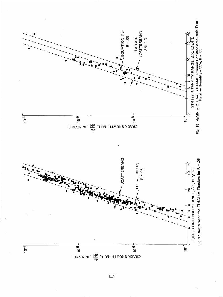
0

0U E

< Ino

<<

c If

o 0 C0- 0 cc

-D E --

00

(0 CI

1t w 4-.olr

Co 00

3-1OA3/-NI' !L!B '3LIv HIMOUD )13VH3

"7p

P = 525 lb

1.6- POL = 656 lb

PMIN = 26 lb

P = 400 lb

SPOL = 500 Ib1.4 PMIN = 201b

1.2- INDICATES ONE OVERLOADCYCLE APPLIED

zw.- 1v lSPECIMEN:

L) 1.0 - AD-25-11

2219-T851 ALUMINUMo CTA

W = 2.5 IN., t =.25 IN.

.8- O/L = 1.25

400 450 500 550

CYCLES, THOUSANDS

Fig. 19 Crack Length vs. Cycles for Overload Tests; O/L = 1.25, 2219-T851 Aluminum

SPECIMEN:AG-25-122219-T851 ALUMINUM

CTB1.6- W = 2.5, t = .25 INCICATES ONE CYCLE

O/L = 1.25 OF POL APPLIED

P = 950 1b, R = 0.1

1.4- P = 8001b P = 5001bPOL = 1000 lb 0 POL = 6251b

P PMIN = 401b

'1.2-

1.-cc

z

.J

S1.0-

.6 I I I I I II

0 20 40 60 80 100 120 140 160CYCLES, THOUSANDS

Fig. 20 Crack Length vs. Cycles for Overload Tests; O/L - 1.25, 2219-T851 Aluminum

118

1.6- P = 950 lb INDICATES 1 CYCLE

IMIN = 50 Ib OF POL APPLIED

1.4

P = 1000 lb-0Q 0 P = 750 lb-*--! POL = 1500 lb POL = 1050lbi _ PMIN= 50Ib PMIN= 401b

1l.2- O/L = 1.5 O/L =1.4

zw_Joe 10o

10-<M SPECIMEN:

ADAG-25-11221A9MT851 ALUMINUM

1.6- CTA

W = 2.5, t =4.25O/L = 1.4, 1.5

.6 1.0 10 20 30 40 50 60

CYCLES, THOUSANDS

Fig. 21 Crack Length vs. Cycles for Overload Tests; O/L = 1.4 and 1.5, 2219-T851 Aluminum

SPECIMEN:AD-25-152219-T851 ALUMINUM

1.6- CTAW =2.51IN., t =.251IN. P = 4001IbO/L =1.5 POL = 600Ib•

S1.4 PM IN = 20 1Ib

z 1.2 - INDICATES ONE OVERLOAD-j CYCLE APPLIED

c• P = 550 Ibn- • •- POL = 825 lb -

010 PMIN = 27.51Ib

.8--

500 550 600 650

CYCLES, THOUSANDS

Fig. 22 Crack Length vs. Cycles for Overload Tests; O/L =1.5, 2219-T851 Aluminum

119

2.0- SPECIMEN:AG-25-2P2219-T851 ALUMINUMCCPW = 6.0 IN., t = .25 IN.

C6,H-- INDICATES ONE OVERLOAD

1.0 - CYCLE APPLIEDz 1.0

-J

C-,

) S =10 ksi

SOL = 15 ksiSMIN = 0.5 ksi

O/L = 1.5

0- 1300 400

CYCLES, THOUSANDS

Fig. 23 Crack Length vs. Cycles for Overload Tests; O/L = 1.5, 2219-T851 Aluminum

SPECIMEN:AD-25-72219-T851 ALUMINUM

1.6 -- CTAW =2.5 IN., t =.25 IN.

-- 1.4 4C6

uJ 1.2 INDICATES ONE OVERLOAD

S1.0- P = 3501Ib

POL = 630 IbPMIN = 17.5 lb

O/L = 1.8.8

I II

1.1 1.2 1.3 1.4 1.5

CYCLES, MILLIONS

Fig. 24 Crack Length vs. Cycles for Overload Tests; O/L = 1.8, 2219-T851 Aluminum

120

SPECIMEN:AG-25-3P

2.0 2219-T851 ALUMINUMCCPW = 6.0 IN., t =.25 IN.

S = 10 ksiSOL = 18 ksi

SMIN = 0.5 ksiO/L = 1.8

S1.0z,,, INDICATES ONE OVERLOAD"CYCLE APPLIED

<

o DATA NOT GATHEREDOVER THESE RANGES

.0800 900

CYCLES, THOUSANDS

Fig. 25 Crack Length vs. Cycles for Overload Tests; O/L = 1.8, 2219-T851 Aluminum

SPECIMEN:AG-25-6P

2.0 2219-T851 ALUMINUM 12.51CCPW = 6.0 IN., t=.25 IN.O/L = 1.25, 2.1 21

STRESSES AS NOTED 12.51

SMIN 0.5 2I-•0.8 ksi I I 12.5 , 12.51 .,.fz9 0.6 12.5 i21

w" INDICATES ONE OVERLOADi I/I CYCLE APPLIED0 IVALUESHOWN IS<• OVERLOAD MAGNITUDE (ksi)

0250 300 350 400

CYCLES, THOUSANDS

Fig. 26 Crack Length vs. Cycles for Overload Tests; O/L 1.25 and 2.1, Aluminumi

121

Inco

N

LLJ En LCV)N

z ii

-UH U)

Li L I

oa_ I. . .U) 0)

0. 0

'--Vzz

S CLU CL LOin1 1 1

F7 3: u) iSý 0co0) CL F- x

LU w (

00~

Cd*4

Vo OC C 00

U) U)

~~z < a

-JJ mE~

0 0

-1 00 in 0

in) -It ODNI 00 6H9J >IDVU-

C122

F-- co

U) -J I

zo~Z LU~1

C.0U,

-ý _ -z Lo z rCN MN D~ 0

CNC 0~ -0

0 H.0~Lo E -j,. 0 0

0Ex 0

01D 2:

<0

(D OD I

LLJ 0

V)~d < C

0 in 0 O

IncoI

wU d)H 0 -zN

H- coo

n-U,wuZ D0j

Z: 0 Cz 0

1ý 1 0 CD n-H H

zl 00 0) -

2: R: )

U, ch O*: 00

U)jd 0 NEX Cu4

0) o Lo

123

CN

~~~0

0

I-

c 0

0

CL

C.D)

E E

LL

0C00

LO)

('N S IOAD V-C)

12

1.10-SPECIMEN:AD-25-112219-T851 ALUMINUMCTAW= 2.5 IN., t=.25 IN.

P = 400 Ib /POL = 500 Ib /

PMIN = 20 IbO/L = 1.25 /

1.05 /

z

zuJ-J

0

1.00

/ INDICATES ONE OVERLOADCYCLE APPLIED

DATA

CONSTANT AMPLITUDE

/ CALCULATION

.95-

400 450 500

CYCLES, THOUSANDSFig. 32 Crack Length vs. Cycles for Overload Tests; O/L = 1.25, 2219-T851 Aluminum

125

AA

20•SPECIMEN:

• * AD-25-101

16- A *2219-T851 ALUMINUM

SA * a AT OVERLOAD (IN.)C-) * 1.094b 12- A A 1.124

C6 A

8 t * APPLIED ONE CYCLEOF OVERLOAD.

A O/L =1.25

4 A•

0 0I I I II

0 1 2 3 4 5CYCLES, THOUSANDS

Fig. 33 Crack Length vs. Cycles, O/L = 1.25

SPECIMEN:AD-25-1 01

10- 5 TEST 1

A TEST 285 TEST 3

8 A

j 6

£5 A

2-

2 4 6 8 10 12 14 16 18 20

Aa SINCE OVERLOAD, 10-3 IN.

Fig. 34 Instantaneous A a/A N vs. A a after Overload

126

12- /SPECIMEN:

AD-25-1 01

w * TEST 1J 10 TEST 2

10 A TEST 3

z Acob 8

6--

w A A A

< A A_ A

D A *

o A

2

I I I I II I I

0 2 4 6 8 10 12 14 16 18 20

A/a SINCE OVERLOAD, 10-3 IN.

Fig. 35 Cumulative A a/A N vs. A a after Overload

10SPECIMEN:

AD-25-101

w 0 TEST 1-J A TEST 28-

A TEST 3zCo 4 AA

* 4

w (4-

w

2

U I I I I I I

0 4 6 8 10 12 14 16 18

Aa SINCE OVERLOAD, 10-3 IN.

Fig. 36 Average A a/A N vs. A a after Overload

127

12

A Kbase = 15 ksi (IN)½104

8- AKpeak 20

Zj Npeak 5

'6-

4,,ý ASSUMEDBEHAVIOR

2-

0 0I1 10 100 1000

CYCLES AFTER PEAKa)

10

8

LU6J

C0

4-

2-

0 I I I

0 100 200 300 400 500 600 700 800

CYCLES AFTER PEAKb)

Fig. 37 "Typical" Crack Growth After An Overload

128

KC

a. Cycles after PeakKc

b. Crack growth after PeakFig. 38 Variation of Kc after Overload

5000 -

0/

-/

z //

_ozLU

X 2500 /LUtre

/i INCLUDED

"" ~HIGHLY TRANSIENT BEHAVIOR ECUE"- ,,-

0

0 500 1000CYCLES

Fig. 39 Calculated Crack Growth With and Without Highly Transient Behavior

129

1250-

SPECIMEN: AD-25-43

OV ERLOAD CYCLE

1000-

750-m ~+10 +5 0

CYCLES AFTER +1 +2 +3 +100 +500 +750 +1000

OVERLOAD0

500-

250- ,, . t i~ ~ ' '

0a) MODIFIED DISPLACEMENT VOLTAGE, (ClVd - C2VL)

1250

1000

750_ CYCLES AFTER -1 +1 +500 1,000 -1 +500 +1000

OVERLOAD

0

500-

2501 I I

0 I I __MODI FI ED DISPLACEMENT VOLTAGE, (ClVd - C2 VL)b)

Fig. 40 Crack opening Traces, Periodic Overload

130

SPECIMEN AD-25-432219-T851 ALUMINUM Pmax Pmin CYCLES

CTA, W = 2.5 IN., t =.25 IN. (Ib) (Ib)

1170 33 1650 33 1000

600MEASURED CLOSURE LOAD

000 0

400 - '0. 0 0 0

00

200 -

010 40 80 120 160

CYCLES, THOUSANDS

Fig. 41 Crack Opening Load vs Cycles, Periodic Overload

z

"TS1(R0TEST 2 -PERIODIC OVERLOAD-o TEST 1 (R =0)

w OL =P O/L

R 0

II0

K1 K2 Ak KSTRESS INTENSITY RANGE, AI K, ksiV-

Fig. 42 Periodic Overload and Constant Amplitude Tests

131

z TEST 3 (R f0) TEST 1 (R= 0)0 TEST 2 (R=0)

Ld

rr"

0

V

o<

I )

A K3 K1 AK

STRESS INTENSITY, K, ksiA/Th.

Fig. 43 Effect of Stress Ratio Changes

z

-O

'0 R > Rcutoff R =R

uJcc

0<•

C- I II I

o I

A Kex A K AK

STRESS INTENSITY RANGE, K, ksiV-N.

Fig. 44 Evaluation of Extreme Rate Curve

132

A Kth A Keffth

I1 i-Cf0

>:

tU)zw

I--fz

W AKeffth IC,)

Rcutoff STRESS RATIO, R

Fig. 45 Variation of A Kth with Stress Ratio

SPECIMEN: AD-25-45 AD-25-26O/L =1.25 O/L 1.8

10-5

-J

zz

"0

I-

0

C-,

10 20 30 40 50

STRESS INTENSITY RANGE, A K, ksiV"i-.

Fig. 46 Periodic Overload Test Comparison

133

SPECIMEN:TG-25-1 01Ti 6AI-4VCT B

1.5 W=2.5, t =.251.5 -

P =1000 lb

POL = 1500 l bPMIN 75 Ib

•1.3-

(Dz

Uj.9

INDICATES 1 CYCLEOF 1500 lb APPLIED

60 80 100 120 140 160 180 200 220

CYCLES, THOUSANDSFig. 47 Crack Length vs. Overloads for Single Overloads; O/L =1.5, Ti 6AI-4V Titanium

SPECIMEN:1.8- TG-25-11

Ti 6A1-4VCT B

W =2.5, t=.25I1.6-P = 10001b

OOL =01800 lb1.PMIN = 751b

1.2-

1.0I INDICATES 1 CYCLEJr OF 1800 lb APPLIED

.810 100 200 300

CYCLES, THOUSANDS

Fig. 48 Crack Length vs. Cycles for Single Overloads; O/L = 1.8, Ti 6AI-4V Titanium

134

M U)

<. D

-J NN*NAg~

iLi

< U) cU) -

000 Co Q Z0 Cof)Q

-P - -2

Co

10 14 00 -0 0 10 C, 0 *I0

CCo

Co Q 0 Ua C/3 0

wL 0 >1 zi

V) Cor 0

N0 0ct 0

0 00-~ 00c

'N1 'e 'HI9N31 )IOVHO

'35

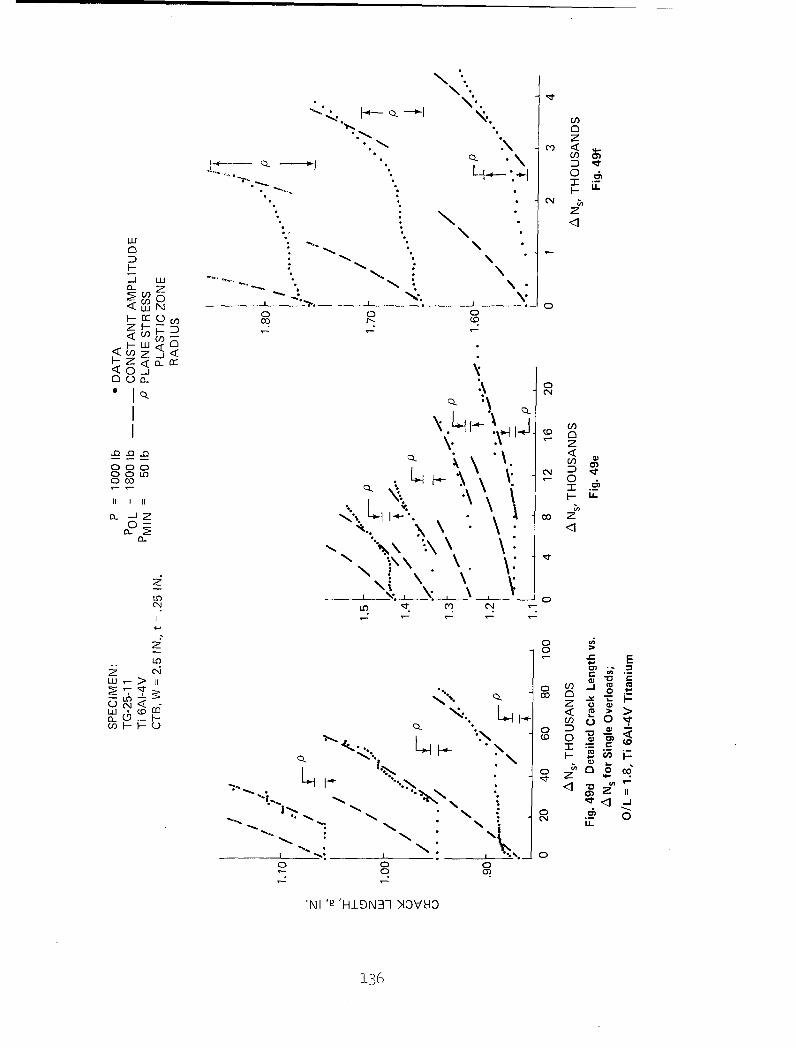
I.-

IN. Z

0) 0w0u N

F- cc, a- *\

zz

F-w <

Lc- 0

0: \

0

LO -j z 00

..

IN 't

N .2

0 0 CDL, 0)0

N1~~~ 'aIDT )~U

136o

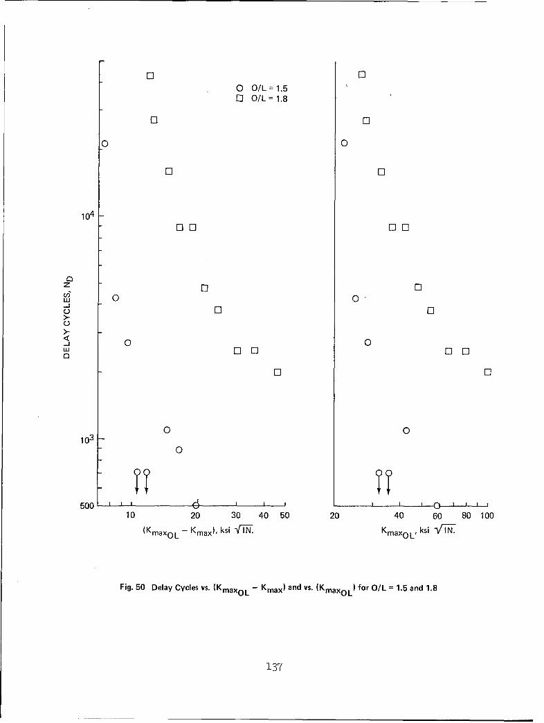
0 O/L = 1.50l O/L = 1.8

00

104

El- El ElE

Ci

0103

000

10 20 30 40 50 20 40 60 80 100

(KmaxOL - Kmax), ksi IKmax 0 ksi -VTI N.

Fig. 50 Delay Cycles vs. (KmaxOL - Kmax) and vs. (K maxOL) for OIL = 1.5 and 1.8

'37

1.8 POL P R N

SPECIMEN (Ib) (Ib) (CYCLES)

o TD-25-30 1870 1040 .05 500 O

1.6 0 -37 1440 800 .05 500+ -28 1440 800 .05 10003 1.4- N 0,/

F- POL-(2'z

O 1.2

1.0

.80 100 200 300 400

CYCLES, THOUSANDS

1.8

1.6

F-

z 1.4w-J

n 1.2

1.0

.8 I I I I0 200 400 600 800

CYCLES, THOUSANDS

Fig. 51 Crack Length vs. Cycles for Single Periodic Overloads, O/L 1.8, Titanium

138

- EIc

Ci

0

o U c

-1 0 00

CD~C C Dcm

00 00 0

000 CL

0~. 000

0 Uý

T-6i LL

Ln L

ciA CCNC

00

'39

0 cCd, 0

06~

0 I

000

0000 00

01 0000 lzr0 0 0

00

2ý00~- 0

00-z

00< LO C14'~-~ 0 CN

0 0U

1d F- .10

0 0Z)0 0

0i < 0

00MI

10 O

S .2

40

w U000

Z 0) LO LOO -

0-

0 0 0

000 000 0000

<00 .2

0 0 00 ~0 ng

0~ *0.0 0

-LO)

z~ UJCNN

- U ) .0

SON

<0<0

on FnC, )u

00 LO

3-10kO/HNP 3- HIMOHD )NDV80 TDVH3AV

1~40

10-4 -

EQUATION (c)

USING R = .0278AND AK= AKOL

w 0-J

1lO-5-z 0

00

I--< 0- 0 0F- 0 0A

AA0

H 0

So Ao A A

0.Uj 0S10-6 -

,<w POL P R N

< SPECIMEN (Ib) (Ib) (CYCLES)

*TD-25-28 1440 800 .05 1000-30 1870 1040 .05 500

o -37 1440 800 .05 500

10-71 1

20 30 40 50 60 70 80

A KOL, ksii'ifN.

daFig. 55 -N-vs. A KOL for Single Periodic Overloads, OIL = 1.8, Titanium

141

SPECIMEN:32 0 AD-25-105

0 SINGLE O/L28 0 ao =.778 IN.

0 POL = 1170 lb24 0 Pmax = 650 Ib

0 Pmin = 32.5 Ib

S20 0Y 0b 16 0

Cu 0<1 12 0

08 0

040

0 [0- L- L L L0 1 2 3 4 5 6 7 8 9 10 11 12 13 14 15

ANs, THOUSANDS

a)

SPECIMEN AD-25-105

FIRSTO/LAPPLIED AT: ao=1.051 0 POL = 11701bao=1.0 7 6 El Pmax = 650 lbao= 1.10 2 A Pmin = 32.51bao = 1.202 0ao = 1.235 C>

SECOND O/L AT Aa = .010SECOND O/L AT Aa = .00628 0 0

0 El A 0 024 0 -l A 0 0

0 El A 0 <2z 20 0 El A 0 C0.7 El A 0 <2C16 0 El A 0 0

0 El A 0 0<112 0 El A 0 0

0 l A o0 08 0 El A 0 C

o El A 0 C>4 El A 0 C>S, El A 0 C>0 i I I I I I I I i I

0 0 1 2 3 4 5 6 7 8 9 10 11 12 13 14 15El 0 1 2 3 4 5 6 7 8 9 10 11 12 13A 0 1 2 3 4 5 6 7 8 9 10 11 A0 0 1 2 3 4 5 6 7 0

C> 0 1 2 3 4 5

b) A Ns, THOUSANDS

Fig. 56 Detailed Crack Growth vs. A NS for Single Overload Interactions, 2219-T851

142

0 33 x 10-6

12 SPECIMEN:

AD-25-105

10 a = 1.051 - 1.077

O/L SEPARATED BY .006S8 POL = 1170 lb

P 8max = 650lb 0

"" Pmin = 32.5 lb e.025oalz 6

170 Ib 1170 lbOVERLOAD OVERLOAD

2 f - - f t0 2 4 6 8 10 12 14 16 18 20 22

CRACK LENGTH, a, 103 IN.a)

SPECIMEN:AD-25-105a = 1.076 - 1.102

O/L SEPARATED BY .00610* POL = 1170 lb

- Pmax= 650 lb6 - Pmin 32.5 lb 0

"1170 lb 1170 Ib- OVERLOAD OVERLOAD * •

21 - f0 2 4 6 8 10 12 14 16 18 20 22

CRACK LENGTH, a, 10-3 IN.b)

34 x 10-5

t 4SPECIMEN:

10- AD-25-105a= 1.102- 1.124

z 8- O/L SEPARATED BY .06

POL = 1170 lb6 max= 6501b

Pmin= 32.5 lbMIZ. z 11701b 11701b * * *

OVERLOAD OVERLOAD

21 - i i p i0 2 4 6 8 10 12 14 16 18 20 22c) CRACK LENGTH, a, 10-3 IN.

Fig. 57 Measured Crack Growth Rate vs. Crack Extension for Single Overload Interactions, 2219-T851

143

40 SPECIMEN:AD-25-102

36 FIRST OVERLOAD APPLIED AT: SECOND O/Lao = .9010 ao = .983 0 ATAa=.006

32 ao = .931] ao = 1.1300 0-0

28- POL = 11701b 0 0Z Pmax= 6501b 0 E 0

C) 24 Pmin 32.5 1b 0 El0 El OK

20 0 El 00 El >

16 0 [] 0 0K SECOND O/L0 El 0 AT ,a =.010

12 0 E00 El0 C

8- 0 El 0 00 El 04 - 0 El 0 K

0 ElDLEG END 0 I I I I I I I I I I I I I I

0 0 1 2 3 4 5 6 7 8 9 10 11 12 13 14 15 0El 0 1 2 3 4 5 6 7 8 9 10 11 12 13 El0 0 1 2 3 4 5 6 7 8 9 0K 0 1 2 3 4 5 6 7

ANs, THOUSANDS

Fig. 58 Detailed Crack Growth vs. A Ns for Single Periodic Overloads, Aluminum

0

SPECIMEN: El40_ AD-25-108

ao= .902 0 SINGLE O.L. 036- ao= .961 El O/L EVERY 2000 CYCLES

ao= 1.167A RECOVERY A

32- 0POL = 2000 lb

7; 28 - Pmax 1600 Ib EA

Pmin 1120 lb 0

b 24

<3 20 0E

16 -0A

12 0 A02 AEl

8 0 A

A4 0

0 ( 1 1t A. I I I I I I I I I I I

0 0 1 2 3 4 5 6 7 8 9 10 11 12 13 14 15 0El 0 1 2 3 4 5 6 7 8 9 10 11 12 13 DA 0 1 2 3 4 5 6 7 8 9 10 11 A

A Ns, THOUSANDSFig. 59 Detailed Crack Growth vs. A Ns for Single Overload Interactions, Aluminum

144

1.8

2219-T851 ALUMINUMSPECIMEN AD-25-12

1.6 -

z CONSTANT AMPLITUDE Ad?a; R = 0.05

E 1.4 Pmax = 450 lb.Pmin = 22.5 lb. N 1730

zw-J

v 1.2c: • N -880

1.0 0 *e A MULTIPLE OVERLOAD0 N30BLOCKS OF N CYCLES

N=3020 Pmax = 675 lb.

Pmin = 22.5 lb.

0.8 L L L L6.50 6.55 6.60 6.65

CYCLES, MILLIONS

Fig. 60 Aluminum, a vs N for Multiple Overloads, R = .05

1.8 2219-T851 ALUMINUM

SPECIMEN AD-25-20 01.7

1.6 CONSTANT AMPLITUDE 0z R = 0.50

4 15 Pmax = 7 0 0 lb.

:- 1.4 Pmin = 350 lb.

zw-j 1.3-

N 640< 1.2 -

1.1 0 l

1.0 - 0000 o•0 N=1010 A MULTIPLE OVERLOAD

0.9 - BLOCKS OF N CYCLES

0.8 0 • N =1550 Pmax = 1050 lb.0.8 *Pmin = 350 lb.

0.7 I I I I I I160 200 240 280 320 360 400

CYCLES, THOUSANDS

a) CRACK LENGTH

Fig. 61 Aluminum, a vs N for Multiple Overloads, R = .50

145

1050,1

800J

S

700 Pmax 700 lb.0

(a DURING OVERLOADA BUMP 1

6008- o BUMP 260A A AFTER OVERLOAD

m (ONE BUMP ONLY)

-AJ

0 500

PRIOR TO OVERLOAD ACLOSURE LOAD AT •

A400 OR BELOW Pmin A A

A6 A

A~ AAAA APmin= 350 lb. T

300 - REMAINDER OF 7CLOSURE LOADS

AT OR BELOW PminGAGE 1 GAGE 2d = 1.178" d = 1.292"

c) OPENING LOAD DETAIL

FOR ONE OVERLOAD BLOCK

1.40

CONSTANT AMPLITUDER = 0.50

z 1.30 - 'max = 700 lb.cc:" Pmin = 350 lb.

w" 1.20--i

A A MULTIPLE OVERLOAD BLOCK

OF 1010 CYCLESo 1.101.10Pmax = 1050 lb.

Pmin = 350 lb.

1.0 I I I I

300 310 320 330 340 350 360 370

CYCLES, THOUSANDS

b) CRACK LENGTH DETAIL FOR ONE OVERLOAD BLOCK

Fig. 61 (Continued)

146

SPECIMEN AD-25-112

.050 -CRACK LENGTH AT O/L = .899 IN.

.050

.040 -

Aa, IN. 0

.030 00

0.020 o) 0 DATA

A ESTIMATED

0 RETURN TO C.A.0

.010 0

0 AO0A 0

i I I I II I

4 8 12 16 20 24 28 32

AN, Cycles, Thousands

Fig. 62a A a vs A N Since Multiple Overloads, Aluminum

5

4) (D 0Q 0 (

LU-J

SA 0

3 0 0000 (z

00

£2 0 DATA

A ESTIMATED0 RETURN TO C.A.

00

4 8 12 16 20 24 28 32

A N, Cycles, Thousands

daFig. 62b N vs A N Since Multiple Overloads, Aluminum

147

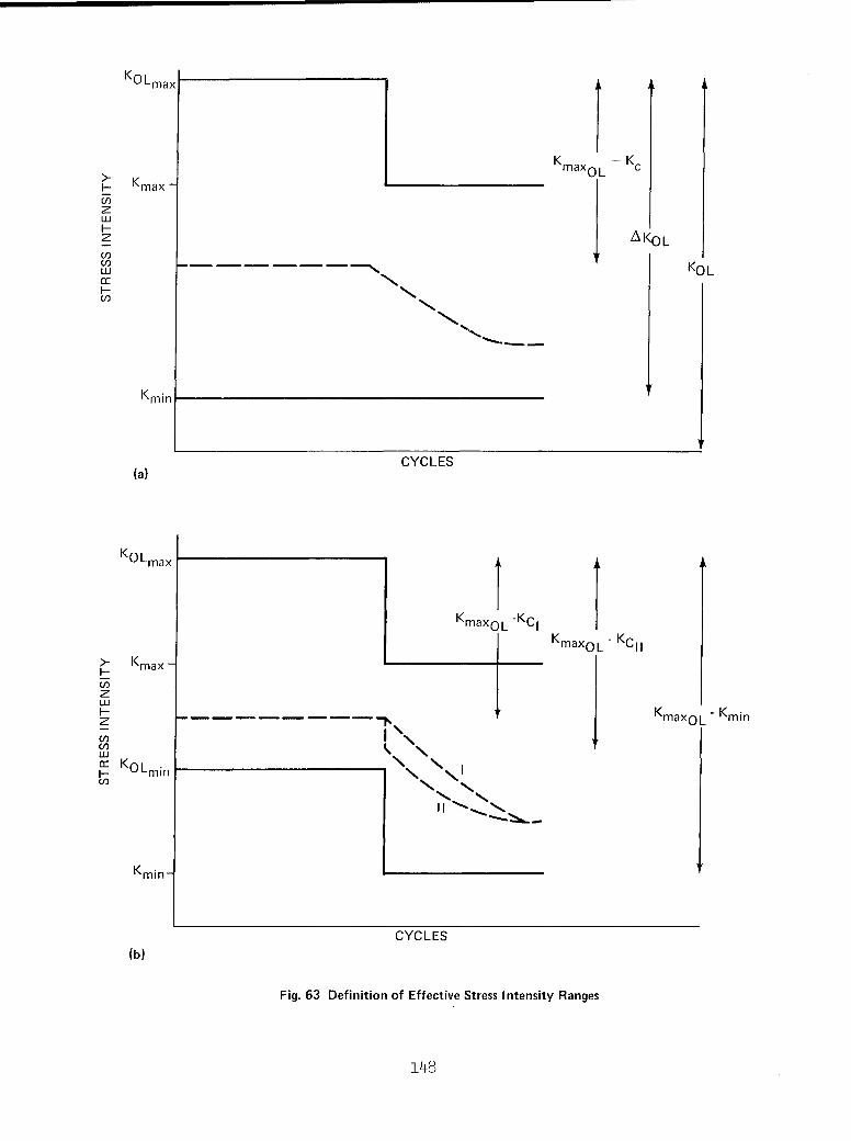
K0 LmaxI

> ma K KmaxO - KC

U)

UU) K0 L

Kmnin

CYCLES(a)

KOLmaxI

KmaxOL- KC,

KmaxOL -KCI 1

zU)wHKmaxOL - min

K0 Lmin N K

Kmin-

CYCLES(b)

Fig. 63 Definition of Effective Stress Intensity Ranges

14t8

- N

0J

0

- o

00

xzco 4-

co

- U.

0

0)

xz00 C?

0 00

U-

(N 0l G )COC

xxcou

149-

C)0

N c

0 b

x

C? 4-

c00

gn

C.,~~- 0 01 _C

0EJ 0

V a,

Ca)

00

OD,U-

NC

10 C0

05

1 [KmaxOL- KCII]2

USING - x21r o y2

12

11 0Z

10-

9-

"' 7- GO

2 6-0

<O

5-

4- ® ®0

3- 0

2--

1-

0~

0 1 2 3 4 5 6 7 8 9 10 11 12

Aa* CALCULATED, 10-3 IN.

Fig. 68 •a* Measured vs A a* Calculated for A K eff (Rmin)

51

TITANIUM SPECIMEN TD-25-21

SCONSTANT AMPLITUDE1.5 Pmax = 12001b

Pmin = 600 Ib SR =.5 •1.•4

6 1.3 -

S_,i• •NO 738

S1.2

wU 1.1

.1.001 dJ . A MULTIPLE OVERLOADS

*9 NOL = 5 3 0 OF NOL CYCLES ATPmax = 1800 lbPmin = 600 lb

.8 O/L = 1.5

250 300 350CYCLES, THOUSANDS

Fig. 69a Crack Length vs. Cycles for Multiple Overloads, R .50, Titanium

SPECIMEN:

1800 -ITD-25-21 POL = 1800 lbs

1700

1600

1500 GAGE •GAGE NO. 1 G-AG-- NO. 2

1400 - d0.959" d 1.079" I GAGE NO. 4

1300 d = 1.382"

1200 S Prnax 1200 lbs

0O 1100 (b LE.J0 LEGEND:

1000 o DURING OVERLOAD

BETWEEN OVERLOADS900 ATRANSIENT

S STEADY STATE800 A A

70 S CLOSURE AT A A CLOSURE AT700 6 lb . AORBELOWPmýý L / ORBELOWPmin

600 min 600 b

250 300 350CYCLES, THOUSANDS

Fig. 69b Crack Opening Load vs. Cycles for Multiple Overloads, R = .50, Titanium

152

1.8 Ti 6AI-4V

SPEC. NO. TD-25-5

1.6 CONST. AMPLITUDE

C6 ~~R = 0.05 O 4,3I- 1.4 Pmax 650 lb

L9 ~~~Pmin = 32.51lb/ -- --- •ozw"j 1.2

/ NO= 27,070

10 MULTIPLE OVERLOADNo , 26,8 on, BLOCKS OF NOL CYCLES"OL-26,800 Pmax= 812.5 lb

0,8 Pmin = 32.5 lb.• I I n n I I

3.60 3.65 3.70 3.75 3.80 3.85 3.90 3.95 4.00

CYCLES, MILLIONS

Fig. 70a Crack Length vs. Cycles, Multiple Overloads, R = .05, Titanium

1.5

;•1.4 0

-- CONST. AMPLITUDER = 0.05

13-- Pmax= 650 IbPmin 32.5 lb"' I

-J 1.2

O L = 27,0701. MULTIPLE OVERLOAD

0 1O1 VBLOCKS OF NOL CYCLES

e Pmax = 812.5 lb1.0 * Pmin = 32.5 lb

I I I I I I

3.84 3.86 3.88 3.90 3.92 3.94 3.96 3.98

Fig. 70b CYCLES, MILLIONS

1000

PmaxOL 821.5 lb •.UPPER BUMP

800- A LOWER BUMP

. Pmax 650 lbI a STEADY STATE

0600 NO CLOSURE,RECORDS TOO NONLINEAR0

400 *. . . .

"0o GAGE 2

200 d = 1.265"-GAGE 1 d = 1.145" 0. -0

Pmin 32.5 lb

3.84 3.86 3,88 3.90 3.92 3.94 3.96 3.98

CYCLES, MILLIONS

Fig. 70c

153

1.230

SPECIMEN:

TD-25-102

1.220 R =.05

*POL =1350 lb

6 max 900 lb

• 1.210 Pmin 45 Ib

zw-J

0< 1.200

1.190

NOL =2

1.180 0

142 146 150 154

CYCLES, THOUSANDS

Fig. 71a Crack Length vs. Cycles for Multiple Overloads, NOL = 2, Titanium

1.160

1.150

z

C6

1.140zw-j

cc 1.1300

1.120 NOL= *

1.110 I I I

134 136 138 140 142 144 146 148

CYCLES, THOUSANDS

Fig. 71b NOL =5

154

1.100

1.090

c 1.080I.-

z0Luw

v 1.070

1.060

NOL= 10o

1.050126 128 130 132 134 136 138 140 142

CYCLES, THOUSANDS'

Fig. 71c NOL = 10

1.045

1.035 -

I- 1.025 -zw-U

,• 1.015

1.005

NOL = 20'

.995118 120 122 124 126 128 130 132 134

CYCLES, THOUSANDS

Fig. 71d NOL = 20

155

.985

.975 -

H .965

zwV0

L)0

< .955 -L)

.945 S

NOL 50

O I I.935

105 107 109 111 113 115 117 119 121

CYCLES, THOUSANDS

Fig. 71e NOL 50

.935

.925 -

Z

C6

CD .915zwI--

< .905

0Irl

.895 NO L 100

.885 I I I I92 94 96 98 100 102 104 106

CYCLES, THOUSANDS

Fig. 71f NOL = 100

156

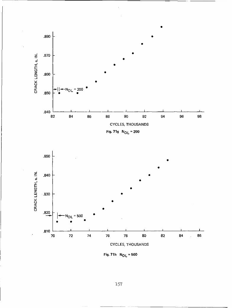
.880 S

z .870m0

3-

z .860-j

US,,

I- NO L 200 0o .850 0 0

.840 I i I

82 84 86 88 90 92 94 96 98

CYCLES, THOUSANDS

Fig. 71g NOL = 2 0 0

.850

-E .840 -

z"_ .830.82 0

0 0

W .810 0

-,J

vS

C,<

.8200-. t. -" NOL =500

.810 tIIIIIII

70 72 74 76 78 80 82 84 86

CYCLES, THOUSANDS

Fig.71h NOL=500

157

.7500 SPECIMEN:

TD-25-115R R=.3

.740- 500 O/L CYCLES

z POL = 1929 IbSPmax=

1286 lb* Pmin = 386 lb

H .7300DzUJ

< .7200C-)

.710-

[--NOL = 500

.700 I I I100 102 104 106 108 110 112 116

CYCLES, THOUSANDSFig. 72a Crack Length vs. Cycles for Multiple Overloads, NOL = 500, Titanium

.800-

.790

S.780I- 0

zw-j,J 0

.770

S-•1I"*-NO L =200

0.760

.750114 118 122 126 130

CYCLES, THOUSANDS

Fig. 72b NOL = 200

158

.850 -

.840

mS

'. .830

zI'-

LuI.820w

_q NOL= 100.810 0

.800

124 126 128 130 132CYCLES, THOUSANDS

Fig. 72c NOL =100

.910

.900

.890

091

zLu

v .880

<

I-

.870NO L =50

.860

134 136 138 140 142CYCLES, THOUSANDS

Fig. 72d NOL = 50

159

.970

.960

j .950l-(9zw-j

yv .940

.930

NOL 20

.920 I144 146 148 150 152

CYCLES, THOUSANDS

Fig. 72e NOL = 20

1.030

1.020

m5

I- 1.010zw-J

0< 1.000

.990

NOL = 10 APPLIED AT151,000 CYCLES

.980 I I 1 1

152 154 156 158 160CYCLES, THOUSANDS

Fig. 72f NOL = 10

160

1.170 -

1.150

:z:"

7.F- 1.130

zLu

-J

S1.110C-"

o0

1.090

NOL = 5 APPLIED AT 159,000 CYCLES

1.070160 162 164 166 168

CYCLES, THOUSANDS

Fig. 72g NOL =5

1.270 -

1.250 -

I--L 1.230zLU

' 1.210C-,.

1.190

NOL = 2

1.170 1 1

165 167 169 171 173

CYCLES, THOUSANDS

Fig. 72h NOL = 2

161

SPECIMEN:AD-25-1152219-T851 ALUMINUMCTA, W = 2.5 IN., t =.25 IN.

1.6 P = 800 IbPmin = 400 lb

POL = 0,1200 lb 5TH O/L *

1.4 1200 4 L

4T O/LL1.2 00-*000 1. .04O

z 3R 2ND O/LU TIME 2DO-j

1.0 T1ST O/L

< 1.0- ~ ~TY IF so

50 100 150 200CYCLES, THOUSANDS

Fig. 73 Crack Length Data for Underload/Overload Spike Sequence, 2219-T851 Aluminum

SPECIMEN:AD-25-1162219-T851 ALUMINUMCTA, W = 2.5 IN., t =.25 IN.

1.6 P = 800 lbPmin = 400 lbPOL = 1200, 0 lb

Z 1.4 1200 NOL

ci 800z 00- 1.2 -J 400'-j

1.0- NOL = 1 * .

S gO

.8 o

100 150 200

CYCLES, THOUSANDS

Fig. 74 Crack Length Data for Overload/Underload Spike Sequences, 2219-T851 Aluminum

162

SPECIMEN:TD-25-119Ti 6AI-4V TITANIUMCTA, W = 2.2 IN., t =.25 IN.

2100

1.2 - 1400

2z 0J 700 •

0 001-- 1.0 - 0i i

z 00(.9.

I00000C- 0

< .8- * 0c 000

.6 t

160 170 180 190 200 210 220 230 240

CYCLES, THOUSANDS

Fig. 75 Crack Length Data for Overload/Underload Spike Sequences, Ti 6AI-4V Titanium

SPECIMEN:TD-25-118Ti 6AI-4V TITANIUMCTA, W = 2.2 IN., t = .25 IN.

1.2- 21000

-1400

,1.0 700 3RD O/L.•

w 0 0 0 0S_2ND O/L 0 0 0

0 1ST O/L

.8 o o• 0 0 0 0 0° °

) 000 00

.61 I I I 1 1 a 1 I

80 90 100 110 120 130 140 150 160

CYCLES, THOUSANDS

Fig. 76 Crack Length Data for Underload/Overload Spike Sequences, Ti 6AI-4V Titanium

163

SPECIMEN:TD-25-117Ti 6AI-4V TITANIUMCTA, W = 2.2 IN., t =.25 IN.

2100. - NOL

- 1400.

1.2 o 700.

OL - 10

a: 100 1oO- 1.0I

z I U1

< 0

C 0 °0

20 30 40 50 60 70 80 90 100

CYCLES, THOUSANDS

Fig. 77 Crack Length Data for Multiple Overload/Underload Spike Sequences, Ti 6AI-4V Titanium

SPECIMEN:AD-25-1172219-T851 ALUMINUMCTA, W = 2.5 IN., t = .25 IN. 1200 NOL

P = 800 Ib 800

Pmin = 400 lbPOL = 1200 Ib <

1.4 0 4000

1.2 103:" 1.2o•°°

z 0

~~1100 010- 1 O0 •g

0 NoL 50<• 0 0 0 0 0O 0 00 '

wI •1 0 0 OS0

.8 I I p

0 10 20 30 40 50 60 70 80

CYCLES, THOUSANDS

Fig. 78 Crack Length Data for Multiple Overload/Underload Spike Sequence, 2219-T851 Aluminum

164

0

0 2 E

00

00

00

00

01

z X, ~LO0 0

CýC11)

Zw<~ 4-0

Z 0>- - N

5:~~co 7 o3 lCý S-0

CLu

CI' 0 (

0N 0 0oCDC

W ~0I 0) o0 o0

'N H0 EN- )D H

Oe~d~f 165

cli

_ * 0

0

O 0 N

o 0 *1*O 6

0ý

LILq

00

C C

LL D 0 o LuU

z 0- 0n 6- U 0 <. E

O - - 0 Lu0~~c I: * *"

CD LU Cc U) Z 'i -< U) -j _j a-,-r)-

0 -L m CL 7C)-l< D UJLLU - (. J

C) C0cl a d

2s (o z

* - 0)

0 0 00O

Z ) C0 j n

LU m

~ E00

'N I 'e 'HILDN3*bovHo 3

166

SPECIMEN:AG-25-9P2219-T851 ALUMINUMCCP, W = 6 IN., t = .25 IN.

Smax= 10 ksiR = 0.05

DATA

CONSTANT AMPLITUDECALCULATION

1.6- (xx) ONE CYCLE OFCOMPRESSION STRESS OFMAGNITUDE xx ksi APPLIEDATZANs =0.

1.4 - (20)

1 .2 -( 5

1.0 (10

• . • _ • ------- " " •(5)

.8-

.6 I I I I

0 1 2 3 4 5 6

A Ns, THOUSANDS

Fig. 81 a vs. A Ns for Compression Spikes, Aluminum

167

* (N

00

00

00 U

0

0 z

a- * 0

L I

CL

C) U)

o .1a- (n N o 0 oC

<J 0

a i (n <± z04<N 0j L .

0 0 <N

0 u~z

0z

LO Z

Loo xNN

a- E

HZ C) * 0

LU COO CC C-t

NI '

168

SPECIMEN:AG-25-9P2219-T851 ALUMINUMCCP, W= 6. IN., t =.25 IN.

Smax= 10 ksi • DATAR .05 CONSTANT AMPLITUDE

CALCULATION(X,Y)TENSILE SPIKE OF

X ksi FOLLOWED BYCOMPRESSIVE SPIKE OF

2.0- Y ksi AT ANs 0

(15, 15)

t 1.81--

1.2

a)- 1.N _ T15OUSANDS

Fig. 83 a vs. A Ns for Tension/Compression Spike Sequences, Aluminum

169

ULJ e'j

2 f<

0 C

Fn~ -i

OCLLO

06 CAu > -

LL 0

CCA

F-

z

0 0

C.)

WL co

H LL.

< 0

<0

2< -

< o CA

C A)

2*J

CL- II

F- i *

W0 Co

CjLh E(n < 0- U) 1\1 Co Co- 1

'N1 'HIONT1 )IOVHO

170

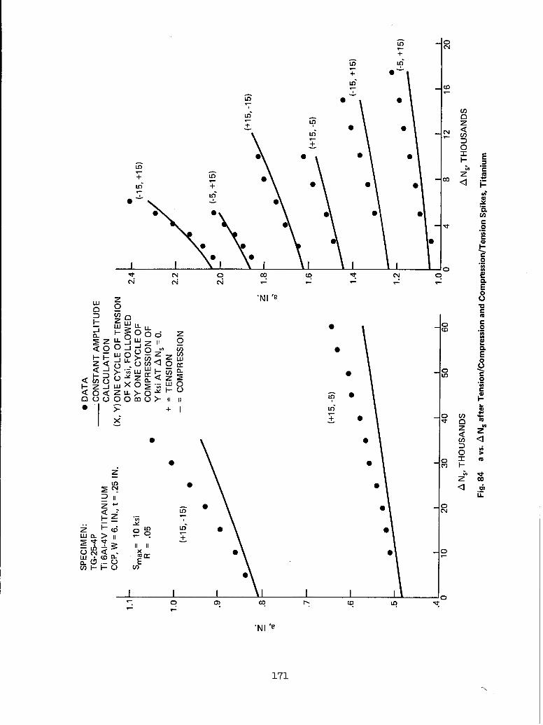
Gin

L6 ~C/

+ 0

Gi

- Z 00+ n6 U

L + 00 0 ~ *6

C2 q C

0 0"00

(N LL- -D E.0

N< 'e 0 J w C)

0 0

W<'luw-l.. 0

LU L)

F-Z) ~~ir 0O

0<J Z- L >- H 0. * 0

a- W) 00 0 m U,)

+ LO 4

+ 0

0

in 0Z co

< -' - 00

-- .ý 0GeP0 06L) L

uj (0CL(D C-) En F- P -) U)

0 CD 00 C. LOi

'N1 'B

171

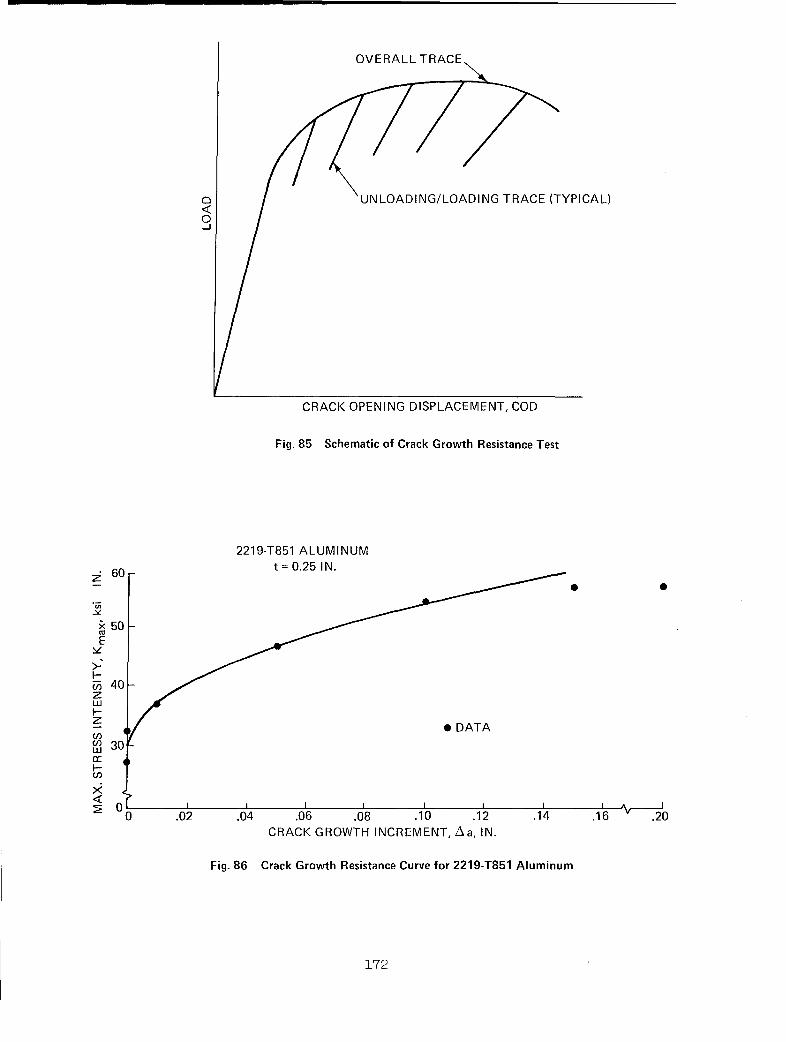
OVERALL TRACE

o •UNLOADING/LOADING TRACE (TYPICAL)

0-J

CRACK OPENING DISPLACEMENT, COD

Fig. 85 Schematic of Crack Growth Resistance Test

2219-T851 ALUMINUM60-t =0.25 I N.S60

0 0

i<50E

zLU

z ODATA

U)cr 4

0 .02 .04 .06 .08 .10 .12 .14 .16 .20

CRACK GROWTH INCREMENT,/Aa, IN.

Fig. 86 Crack Growth Resistance Curve for 2219-T851 Aluminum

172

a 0 TUNNELING DURING OVERLOAD

SPECIMENPROPAGATION THICKNESS

DIRECTION (.25 IN. NOM.)

CRACK FRONT: BEFORE OVERLOADAFTER OVERLOAD

Fig. 87 Schematic of Crack Front Tunneling

//

p

g o-' 100S.90 2

z-w

0a ASSUMEDo ~< ,<o HALF CRACK LENGTH ATcc .0o MID-THICKNESS - O

SOSURFACE LENGTH"" ~(MEASURED)

.85- T 0 0 0 0 00000000

TUNNELING DURING OVERLOAD, at

I I I I I I I I I I I325 330 335

CYCLES, THOUSANDS

Fig. 88 Assumed Crack Front Behavior After Tunneling

173

2219-T851 CCP

a AT OVERLOAD = .852 INCH

KmaxOL = 36.3 ksi IN.

1.0 S = 10 ksiUcSOL =21 ksic- LU\ Samin= 0.5 ksi

SrO

.05 .10

CRACK GROWTH INCREMENTAFTER OVERLOAD, IN.

Fig. 89 Normalized Crack Growth Rate vsCrack Growth Increment After Overload

Ti 6AI-4V TITANIUM

t =0.25 IN.

>- 80---

Uzi 70"Z

U- 60

HE 0 DATAulV 50

0 .02 .04 .06 .08 .10 .12 .14

CRACK GROWTH INCREMENT, Aa, IN.

Fig. 90 Crack Growth Resistance Curve

for Ti 6AI-4V Titanium

174

NOL=100 N=1000O/L = 1.5

1.200- t = .25 IN., SPECIMEN TD-25-50 POL = 1350 lb.t = .75 IN., SPECIMEN TD-75-1 POL = 4,050 lb.

1.100 -

a, IN.

1.000 0

* $

.900-10

.800 - i i i F0 10 20 30 40 50 60 70 80

A CYCLES, A N, THOUSANDS

Fig. 91 a vs A N for Multiple Periodic Overloads for Two Thicknesses

1 .2 l 0 l 0 ,

0

l SPECIMEN TD-25-102

1.1 20 t=.250 W=2.2991N.

0 5 O/L= 1.5Xlw•.oo POL 1 3 5 0 lb., Pmax =900 lb.,

TD-75-2 0• R =.051.0 l~*1 O .0tl 10

1 j SPECIMEN TD-75-2

a, IN. 2 0 t= .75mo 100 0 r- W = 2.496 IN.

.9- 08 0 O 5•750 O/L= 1.5-0 . J 100 TD-25-102 POL 4 0 5 0 lb., Pmax = 2700 Ib.,

S1 5~0 4¶100 R = .058 2K 50 200

* 2K

.7-

SPECIMEN:

TD-75-2 180 220 260 300 340

TD-25-10240 80 120 160 2b0

CYCLES, THOUSANDSFig. 92 Effect of Multiple Overloads for Two Thicknesses

175

DATA: *SPECIMEN TD-25-106 A SPECIMEN TD-75-3

1.3 O/L =1.8 O/L =1.8

POL =1620 LB POL =4860 LB

Pmax =900 LB Pmax =2700 LB

1.2 Pmin 45 LB Pmin 135 LB

t = .250 IN. t =.749 IN.

W =2.200 IN. W =2.497 IN. A

1.1 oe

z gA

1.0 •

SLOPES MATCH A

A

.9 t=%IN.

1st O.L. -. t =¼IN.

.8 [AA A A

0 4th

*A

7 00 3rd

A 2nd

A 1st OVERLOAD

SPECIMEN : I I I I I I I I I

25-106 80 90 100 110 120 130 140 150 160 170 180 190

75-3 150 160 170 180 190 200 210 220 230 240 250 260

CYCLES, THOUSANDS

Fig. 93 Comparison of Crack Growth Rates for Two Thicknesses, 1st Overload

1.3

1.2

000*A

1.1 A

*A

1.0-2:oo° A

.9- AAA S

2nd OVERLOAD *.8 -

0 A

.7 •c oJ

"Aso 2nd OVERLOAD

.6 I I 1 I I 1 I 1 1 I

25-106: 90 100 110 120 130 140 150 160 170 180 190

SPECIMEN: 75-3: 210 220 230 240 250 260

CYCLES, THOUSANDS

Fig. 94 (Continued Fig. 93 2nd Overload)

176

1.3-

SPECIMEN TD-25-106:*

1.2 TD-75-3: A

11 .1

• 1.0 -z r eA AAA

.9 3rd OVERLOAD 0.0

.8-

S3rd OVERLOAD

.6 I I I I I I I ITD-25-106: 90 100 110 120 ' 130 ' 140 150 160 ' 170 180 190

TD-75-3: 240 250 260 270 280

CYCLES, THOUSANDS

Fig. 95 (Continued from Fig. 94) 3rd Overload

1.3

SPECIMEN TD-25-106: e 0

1.2 TD-75-3: A 0

603

1.1 AAA' •4th OVERLOAD

- 1.0 - e[I

.9

,8 *0• 4th OVERLOAD.8

.7 oe. 01

.6 I I II I I I III

TD-25-106: 90 100 110 120 130 140 150 160 170 180 190TD-75-3: 280 290 300 310 320

CYCLES, THOUSANDS

Fig. 96 (Continued from Fig. 95) 4th Overload

'77

SPECIMEN: EB WELDED Ti 6AI-4V TITANIUM

CYCLESSmax PER

-ý .8 (ksi) BLOCK 2

9.4 2860

V

="18.7 1240 0 ~c48 .0

1 IN C H

F- 28.0 497u 6 37.4 141

0 a/c= IL-4"-J 46.7 30o 56.3 1

C.)•0.0 DATA

00LL

EFFECTIVE STRESS MODEL PREDICTION

00 10020304 0BLOCKS

400Fig. 97 Comparison of Data and Prediction Using Effective Stress Model

EFFECTIVE STRESS

RANGE, Z Seff

w RCRACK CLOSUREU) STRESS

\ /

TIME

a) TIP OPEN b) TIP CLOSED

Fig. 98 Schematic of Crack Closure

178

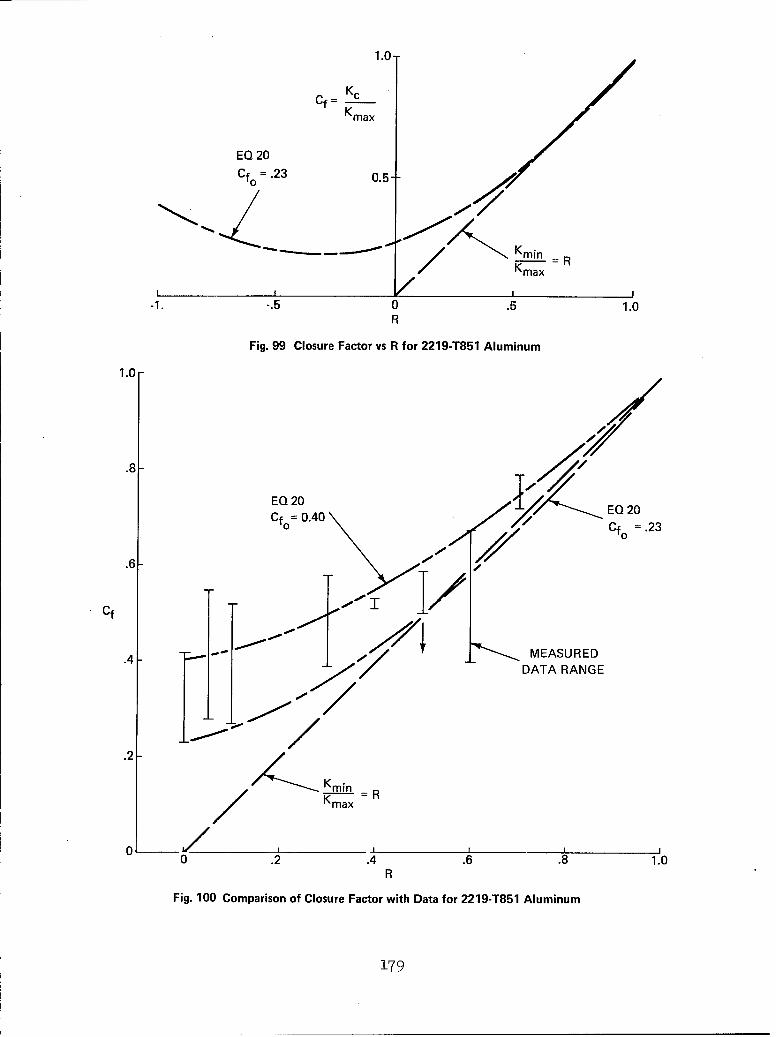
1.0-

Cf= KcKmax

EQ 20

Cfo = .23 0.5

-05

•""•'--• • "Kmin=R

Kmax

__ _ _ _ __ _ _ _ __ _ _ _ __ _ _ _I

-1. -.5 0 .5 1.0R

Fig. 99 Closure Factor vs R for 2219-T851 Aluminum

1.0

.8

EQ 20Cfo = 0.40

.6 //Cf 0 .23

Cf

4 MEASUREDDATA RANGE

KminKmax =R

0 I 1 10 .2 .4 .6 .8 1.0

R

Fig. 100 Comparison of Closure Factor with Data for 2219-T851 Aluminum

179

1.0-/

Cf K _ /Kmax

EQ 21

Kmax

-1. -.5 0 .5

b) TI-6AL-4V TITANIUM R

1.0 //

Kc

_ Kmax

EQ 20 /S~Cfo -=o0.4400-

Kmax

I III

-1. -.5 0 .5R

a) 2219-T851 ALUMINUMFig. 101 Modified Closure Factor vs R

$) o~ca,, i iSc

U)

U)

Sc2

P CYCLES, N,-A a CRACK LENGTH, a

Fig. 102 Schematic of Closure Variation through Effected Length caused by Overload

180

CONSTANT AMPLITUDE CRACK GROWTHRATE (CALCULATED)

z __

I-

MEASURED CRACK0 GROWTH RATE

0p p2

Aa AFTER LOAD CHANGE

Fig. 103 Schematic of da/dN vs Aa After an Overload

/

) PLOT CONSTANT AMPLITUDE /GROWTHTO ESTIMATE p

- /sw•-/

° /0U--

-r•LI.

/ pAa / (ESTIMATED)

1 MODIFY Cf UNTIL INITIAL SLOPE AGREES

ANs

Fig. 104 Schematic of Iteration Procedure to Obtain Cfo

181

1.06- NOL = 20/ SPECIMEN: AD-25-107N*2219-T851 ALUMINUM

1 0 CTA, W = 2.5 IN., t =.25 IN.

* 71.04- • 0 DATA

0 PREDICTION

USING CRACK- "CLOSURE MODEL

1.02 Cfo =.40

0/NOL 50

1.00-

0/0/

.98 -

f .96HN

o I/ 1 P = 650 lb..- 6 POL= 1170 b.

/ * Pmin = 3 2 lb.

S

.92 -

.90 /.NOL 500 /

/.

.881

"80 4 8 12 16 20

Z•Ns, CYCLES SINCE LOAD CHANGE, THOUSANDS

Fig. 105 Comparison of Predictions with Data for High-Low Sequence, 2219-T851 Aluminum, O/L =1.8

1_82

SP

SPECIMEN: AD-25-109 POL S

.94 2219-T851 ALUMINIM • A NsCTA, W =2.5 IN., t =.25 IN. P = 550 lb.

POL= 825 lb.

Pmin= 28 lb.

0 DATAz ~~-PREDICTION 0

S.92 USING CRACK

CLOSURE MODEL

Cfo =.40LU-j

.90 NOL ' o 00cc

.88I I I I I2 4 6 8 10 12

A Ns, THOUSANDS

Fig. 106 Comparison of Prediction with Data for High-Low Sequence,2219-T851 Aluminum, O/L = 1.5

1.2- SPECIMEN: AG-25-12 P 500 lb.

2219-T851 ALUMINUM P POL= 800 lb.

CTB, W =2.5 IN., t =.25 IN. , Pmin = 25 lb.

z 0

H . NOL~-Ow 0

- 0 DATAO• PREDICTION

1.0 I

0 10 20 30 40 50

A Ns, THOUSANDS

Fig. 107 Comparison of Prediction with Data for High-Low Sequence,2219-T851 Aluminum, O/L = 1.6

183

00

LOH<

<- -6 -I ýHH O (N -N

<0

Lu LOLr) 11 - .LO110 11~ *1 Io-4

0

C14 z C

NN MU.-

II -L I-

O %j CZ N 0

(0 ( (l0 in N

U? 0

10 <( 0

II 0 00 ,)*I-) 11 l *

CD c 11 010 HwD -jt_00U

110 E0

rN < 0J3~(,N 0

0 rz H .2c

z *

00

0

00 cNC

z 0

m o C .,( C0 C (CD(N (N - 0 00

184

SPECIMENTG-25-2PTi 6AI-4VCCP, W = 6 IN, t = .25

1.4 NOL= 0 DATA

S = 6 ksi - PREDICTION

SOL = 10ksi USING CRACK

Smin 0.3 ksi CLOSURE MODEL

1.2 O/L = 1.67

1.0 * " -0

a(IN) 7,

.8 0

NOL= 0

.6S = 10ksi

SOL 16 ksi

•-- Smin = 0.5 ksiO/L = 1.60

.4I I I0 40 80 120 160 200

A NS (THOUSANDS)

Fig. 110 Comparison of Predictions with Data for High-Low Sequence, Ti 6AI-4V TitaniumO/L = 1.6, 1.67

185

STRESS

SEQUENCE A SEQUENCE B

A~ ANs CYCLES, N N

SEQUENCE A

SEQUENCE B

k 0 ANS

Fig. 111 Effect of Two Different Load Histories on Subsequent Crack Growth

186

SPECIMEN: AG-25-1P2219-T851 ALUMINUM

6 ksi

6.0-

-4.13.54

S3 4 5 6 7 8 9 10 11 ---- CYCLE NO. 4 t 4 ftR = 0.05

COD

Fig. 112 Load vs COD Sequence for Two Stress Ratios, R = .5/.05

SPECIMEN: AG-25-1P2219-T851 ALUMINUM

1 23R = 0.7

Smax = 6 ksi2c = 5.0 IN.

"T 7-" 6 - CYCLE NO.4 5

R = .05COD

Fig. 113 Load vs COD Sequence for Two Stress Ratios, R = .7/.05

187

STRESS

S1 --- _ _

SS

mm 1 l

mS2Smin, SI P I• c2

Smin2I

CYCLES, N

Fig. 114 Schematic of Minimum Stress Adjustment

CURRENT LOADING: P=951 lb., R =0

LOADING PRIOR TO A NS =0: P=951 1b., R=0.7

SPECIMEN: AG-25-292219-T851 ALUMINUM 0

1.0CTB (W 2.5 IN., t = .25 IN.)

0z .9-LU-J

0 CONSTANT AMPLITUDE

.8- •CALCULATION

0 DATA

.7 1 1 i 10 8 12 16 20

Ns, THOUSANDS

Fig. 115 Comparison of Constant Amplitude Calculation withData For Minimum Stress Variation

188

SPECIMEN: AG-25-302219-T851 ALUMINUMCTB (W = 2.5 IN., t =.25 IN.)

1.3 CURRENT LOADING: P = 951 lb., R = 0.3

LOADING PRIOR TO AN =0: P 91l. .

F- 1.23z

w-J CONSTANT AMPLITUDEle" 0 CALCULATIONC.)

1.1 0 DATA

SI I

0 2 4 6 8A Ns' THOUSANDS

Fig. 116 Comparison of Constant Amplitude Calculation with Data for Minimum Stress Variation

STRESS

S2

Sc2

Scl i_..

0 NSAT CYCLES

NOL

Fig. 117 Schematic of Variation of Closure Stress with Number of Overload Cycles

189

STRESS

N OL CYCLES,

Aas CRACK LENGTH

N OL

F-KNOLN NSAT

3:

0

Cr

0

Aas

190

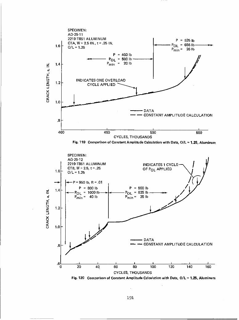
SPECIMEN:AD-25-112219-T851 ALUMINUM P = 525 lbCTA, W = 2.5 IN., t =.25 IN. = 6561.6 O/L = 1.25 POL =65 Ib•

Pmin = 26 lb

P = 400 Ib

•'--- POL = 500 lbz 1.4 Pmin = 20 lb

C6I-

INDICATES ONE OVERLOADz 1.2-u CYCLE APPLIED-J

0

SDATA- - CONSTANT AMPLITUDE CALCULATION

.8

400 450 500 550CYCLES, THOUSANDS

Fig. 119 Comparison of Constant Amplitude Calculation with Data, O/L 1.25, Aluminum

SPECIMEN:AG-25-1 22219-T851 ALUMINUM INDICATES 1 CYCLECTB, W = 2.5, t =.25 OF POL APPLIED

1.6 O/L = 1.25

-.- -o--P=9501b,R=.01

1.4 P = 8001b P = 5001b" PO L = 1000 lb =POL = 625 lb

C6 Pmin = 401b Pmin = 25 lb

I-

z 1.2-j

c 1.0

DATA.8 CONSTANT AMPLITUDE CALCULATION

.6 II I I I I I0 20 40 60 80 100 120 140 160

CYCLES, THOUSANDSFig. 120 Comparison of Constant Amplitude Calculation with Data, O/L = 1.25, Aluminum

191

SPECIMEN:AG-25-112219-T851 ALUMINUM

1.6 CTB, W = 2.5, t =.25 JINDICATES 1 CYCLE

P = 1000 lb P = 7501b OFPOLAPPLIED

1.4 - OL =1500 lb POL = 1050 lbPmin = 50 Ib- b Pmin = 40 lb

-O/L = 1.5 O/L= 1.4

1.2L•P = 950 Ibzu Pmin = 50 Ib-J

< 1.0

.8 . DATA

CONSTANT AMPLITUDE CALCULATION

0 10 20 30 40 50 60

CYCLES, THOUSANDSFig. 121 Comparison of Constant Amplitude Calculation with Data, O/L = 1.4, 1.5, Aluminum

1.6 SPECIMEN:AD-25-1 5 P = 400 lb

CTA, W=2.5 IN.,t=.25 IN. Pmin = 201b

. 1.4 O/L =1.5

Z 1.2 INDICATES ONE OVERLOAD-J CYCLE APPLIEDv

< , _5--•P = 5501IbL) 1.0 PO• ' -- P L = 825 1b _

Pmin = 27.5 lb

DATA.8 CONSTANT AMPLITUDE CALCULATION

500 550 600 650

CYCLES, THOUSANDS

Fig. 122 Comparison of Constant Amplitude Calculation with Data, O/L = 1.5, Aluminum

192

2.0

SPECIMEN: IAG-25-2P2219-T851 ALUMINUMCCP, W= 6.0 IN, t=.25 IN.

f/6 S = 10 ksiINDICATES ONE OVERLOAD SOL = 15ksi

U CYCLE APPLIED /min = 0.5 ksiuz 1.0 Smn= 0. s

O/L = 1.50

__ DATA- CONSTANT AMPLITUDE CALCULATION

300 400

CYCLES, THOUSANDS

Fig. 123 Comparison of Constant Amplitude Calculation with Data, O/L = 1.5, Aluminum

2.2 2219-T851 ALUMINUM

): NUMBER OF DATA POINTS

2.0 Sc AFTER NOL = 11= Sc AFTER NOL = NSAT

0

_j 1.8/,i41) E)(2)QW 1.6 / , ,(1)2

On"

> //

w /20

u.i

Er 1.6

-J

0

/

L ) 1.4 (•12 2/3)17

0 I I I i I

1.0 1.2 1.4 1.6 1.8 2.0

OVERLOAD RATIO, O/L

Fig. 124 Calculated Closure Stress After One Overload over Previous Closure Stress vs Overload Ratio

'93

1.8 - G 2219-T851 ALUMINUM

1.6 -

Rc 1.4- O/L= 1.8

1.2

3 POINTS

1.0 . I I I I0 4 8 12 16 20

NO/L

Fig. 125 Rc vs NOL for O/L = 1.8 2219-T851 Aluminum

1.0 - 2219-T851 ALUMINUM

NSAT.9- 0] 0

7 'A

.8 00 0

O/L01.50 1.8

.7 0A2.1

(9)

NUMBER OF DATA POINTS

.6-

0 4 8 12 16 20

NOL

Fig. 126 Factor -y vs NOL for 2219-T851 Aluminum

1-94

1.2

1.0 (8) 0 0 0 0(2)(12) (2)

0 0

OVERLOADc 0 RATIO

.8 031.5A1.6, 1.6701.8

)NO. OF DATA POINTS

.6 RANGE OF DATA

0100 200 300 400 500 2000

NUMBER OF OVERLOADS, NOL

Fig. 127 Factor y vs NOL for Ti 6AI-4V Titanium

.4

01

STRESS RATIO, R

Fig. 128 Crack Tip Crushing vs. Stress Ratio, R

195

TENSION

Stain 1 - $1____ 2

W S,

0 CYCLES

Smin2

COMPRESSION

Fig. 129 Schematic of Closure Adjustment for Compression Stresses

TENSION

Co Sc-

SI'

CowU) Sc'U)

Smin1

S2

0 •

CYCLES

Fig. 130 Schematic of Closure Adjustment for Underload Spike

TENSION

$1

Sc

Sc' -CoU)wc 0-

CYCLESCn Sminl

$2ý

COMPRESSION

Fig. 131 Schematic of Closure Adjustment for Compression Spike

196

I-x x < c

E E U(n cnC (n cn (n CA

CN 0 00

C14A

wUJ (n -o

z z 0

E -JI

CAN

SS381S

x xco m

E U. EL E UEACA CA CA CA CA c

I 2

(n In = c

0C

CO W 1r 0~

z Eco 114

cli 2

U -1ssh:n

'97

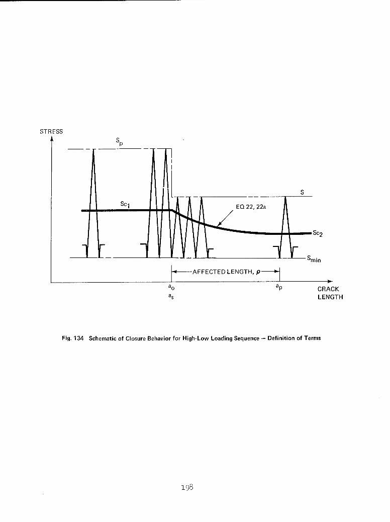
STRESS

Sp

pS

SCl EQ 22, 22a

AFFECTED LENGTH,

ao ap CRACK

as LENGTH

Fig. 134 Schematic of Closure Behavior for High-Low Loading Sequence - Definition of Terms

195

CD

x x c x C DC

E E E E c. E(n, C/) Cin (n )

e'_j

C~j E

I U Z

F <~Vn E 0:

[FI - E

cn C/),

CV)

CV) V)

C/) (n )

(0

I cv

F i C)Cl)

En, CL

av I

ca c

cu 4

NN C.

Fi '-I cv a

LO

199

2.0- SPECIMEN: /AG-25-1P /2219-T851 ALUMINUM /CCP, W = 6.0 IN., t =.25 IN. /

1.9- / 0

/S = 6 ksi

C6 R = 0.5I1.8 CONSTANT AMPLITUDE

LU 10V- 0

L 1.7-<o ool

1.6- ~ DATAPREDUCTION

1.5q

500 520 540 560 580

CYCLES, THOUSANDS

Fig. 137 Predicted a vs. N for R = 0.5, 2219-T851 Aluminum

1.1 SPECIMEN:AG-25-29 02219-T851 ALUMINUMCTB, W = 2.5 IN., t =.25 IN. S

S1.0e -

"c" P = 951 IbSR = 0.0

(D CONSTANT AMPLITUDE

.Z .9.

8• . 0 DATA--- PREDICTION

.7 I I I I I I I I I I200 205 210 215

CYCLES, THOUSANDS

Fig. 138 Predicted a vs. N for R = 0., 2219-T851 Aluminum

200

SPECIMEN:AG-25-7P2219-T851 ALUMINUMCCP, W = 6.0 IN., t =.25 IN.

2.0 S =6 ksi /0

R =-1

/0

• 1.5 -

I- /00z

-j

<o0 1.0-

--- 0

•.5 - "- .--- 0""0" 0 DATAPREDICTION

450 500 550 600

CYCLES, THOUSANDS

Fig. 139 Predicted a vs. N for R =-1, 2219-T851 Aluminum

SPECIMEN:TD-25-17Ti 6AI-4V TITANIUMCTA, W = 2.5 IN., t = .25 IN.

P = 1000 Ib 00R = 0.5 0CONSTANT AMPLITUDE 00 .

.c" 1.1 0-

0S01-

z 0

o 01.0 0 DATAS100 - -- PREDICTION

0

.90 1 I I I I I

140 160 180 200 220 240 260

CYCLES, THOUSANDS

Fig. 140 Predicted a vs. N for R = 0.5, Ti 6AI-4V Titanium

201

SPECIMEN:TG-25-06Ti 6AI-4V TITANIUMCTA, W = 2.5 IN., t = .25

CONSTANT AMPLITUDE1.9 P = 700 lb

R = 0.3

-I

,(1.

600 700 800 900

CYCLES, THOUSANDSFig. 141 Predicted a vs. N for R 0.3, Ti 6AI-4V Titanium

1.6- SPECIMEN:TG-25-02 /

-- Z ~Ti 6AI-4V TITANIUM//eTA, W = 2.5, t =.25D

1.4O ~CONSTANT AMPLITUDE,,z P = 11001b/

-j R = 0.05 -C) ~~PREDICTION-,,

<• 1.2-

c:

1.3

.81

180 200 220 240 260 280 300 320 340

CYCLES, THOUSANDS

Fig. 142 Predicted a vs. N for R = 0.05, Ti 6AI-4V Titanium

202

SPECIMEN:TG-25-5PTi 6AI-4V TITANIUMCCP, W = 6.0 IN., t =.25_I . /

1.5 S= 10 ksi 0 /R =-1CONSTANT AMPLITUDE -

I 0-

_ 1.0 *

.0<0

.5 - - DATA- -PREDICTION

.- - CALCULATED FROMEQUATION 3

0750 800 850 900

CYCLES, THOUSANDS

Fig. 143 Predicted a vs. N for R = -1, Ti 6AI-4V Titanium

SPECIMEN:AD-25-112219-T851 ALUMINUMCTA, W = 2.5 IN., t =.25 IN. P = 525 Ib

1.6 O/L= 1.25 POL = 656 lbPmin = 26 Ib

P = 400Ib /POL = 500 lb

; 1.4 Pmin = 20Ib /

ONE OVROAD--

Z 1.2- CYCLE APPLIED

DATAPREDICTION

.8

I ,400 450 500 550

CYCLES, THOUSANDS

Fig. 144 Predicted a vs. N for O/L = 1.25, 2219-T851 Aluminum, Single Overload

203

SPECIMEN:AD-25-15

1.6 2219-T851 ALUMINUMCTA, W=2.5 IN.,t=.25 IN. P = 400 lbO/L = 1.5 • POL = 600 Ib-

Pmin= 20 lb_z 1.4 /

F-C9 INDICATES ONE OVERLOADwZ1. CYCLE APPLIED-J

< 5 P = 550 Ib

A10 POL = 825 Ib -

S 1.4 5 0 = - /s

Pmin m 27.5 Ib

SDATA.8 • •PREDICTION

I-I A

500 550 600 650CYCLES, THOUSANDS

Fig. 145 Predicted a vs. N for O/L =1.5, Single Overload, 2219-T851 Aluminum

1.8- SPECIMEN:AG-25-2P I

1.6 - CCP, W =6. IN., t =.25 IN. /

S = 1,8

.6min O 5 VER STARTING AT

M-~~~ 1.2 29000 CYCLE500CYLE

1.4-

.- /a:: INDICATES (1) CYCLEOF OVERLOAD,,PPLEo\, '00.,,..6- • / iSTAR TI N GAT

!Y _i"290000 CYCLES

DATA.2- PREDICTION

0 290 300 320 340 360 380 400CYCLES, THOUSANDS

Fig. 146 Predicted a vs. N for O/L = 1.5, Single Overloads, 2219-T851 Aluminum Panel

204

SPECIMEN:

1.6 AD-25-72219-T851 ALUMINUMCTA, W= 2.5 IN., t=.25 IN.

P = 350 Ib

1.4 POL = 630 lbPmin= 17.5 lbO/L = 1.8

INDICATES ONE OVERLOAD

Z 1.2- CYCLE APPLIED

f-J

0 1.0--

DATAPREDICTION

.8 i1.1 1.2 1.3 1.4 1.5

CYCLES, MILLIONS

Fig. 147 Predicted a vs. N for O/L = 1.8, Single Overloads, 2219-T851 Aluminum

2.0-

1.8 SPECIMEN:AG-25-3PCCP, W = 6. IN., t = .25 IN.

1.6 S = 10ksi 4/

SOL = 18ksi

zý 1.4 Sm in =.5 ksi

-O/L = 1.8*

F- 1.2 ××

z *w

J 1.0Sxx/

0 .8 INDICATES (1) CYCLE

OF OVERLOAD 'PeE ,DITIO.6 APPLIED PREDICTION

.- * STABLE TEAR INCLUDEDIN CALCULATIONS

+++++ DATA NOT GATHERED IN.4- THESE RANGES

.2 f I810 850 900 950

CYCLES, THOUSANDS

Fig. 148 Predicted a vs. N for O/L = 1.8, Single Overloads, 2219-T851 Aluminum Panel

205

SPECIMEN:TD-25-13Ti 6AI-4V TITANIUM

1.6 CTA, W = 2.5 IN., t =.25 IN. 0

SO/L =1.25

S1.4•_ o /

z ONE CYCLE OF 0 7w OVERLOAD APPLI ED -"" 0 O DATAS1.2- O -P PREDICTION

0

1.0 1 P = 700 lb P = 850 lbPOL = 875 lb POL = 1063 lbPmin = 35 lb Pmin = 43 lb

.8 1

1.20 1.25 1.30

CYCLES, MILLIONS

Fig. 149 Predicted a vs. N for O/L 1.25, Single Overloads, Ti 6AI-4V Titanium

SPECIMEN:1.7 - TG-25-10

Ti 6AI-4V TITANIUM ICTA, W = 2.5, t =.25

1.5 - oP = 1000 lb PREDICTION -,-/

1. min = 75 IbSIIO/L= 1.5•- 1.3

zw-J

S 1.1DATA

INDICATES 1 CYCLEOF 1500 Ib APPLIED

.7 1 1 1

60 80 100 120 140 160 180 200 220

CYCLES, THOUSANDS

Fig. 150 Predicted a vs. N for O/L = 1.5, Single Overloads, Ti 6AI-4V Titanium

2o6

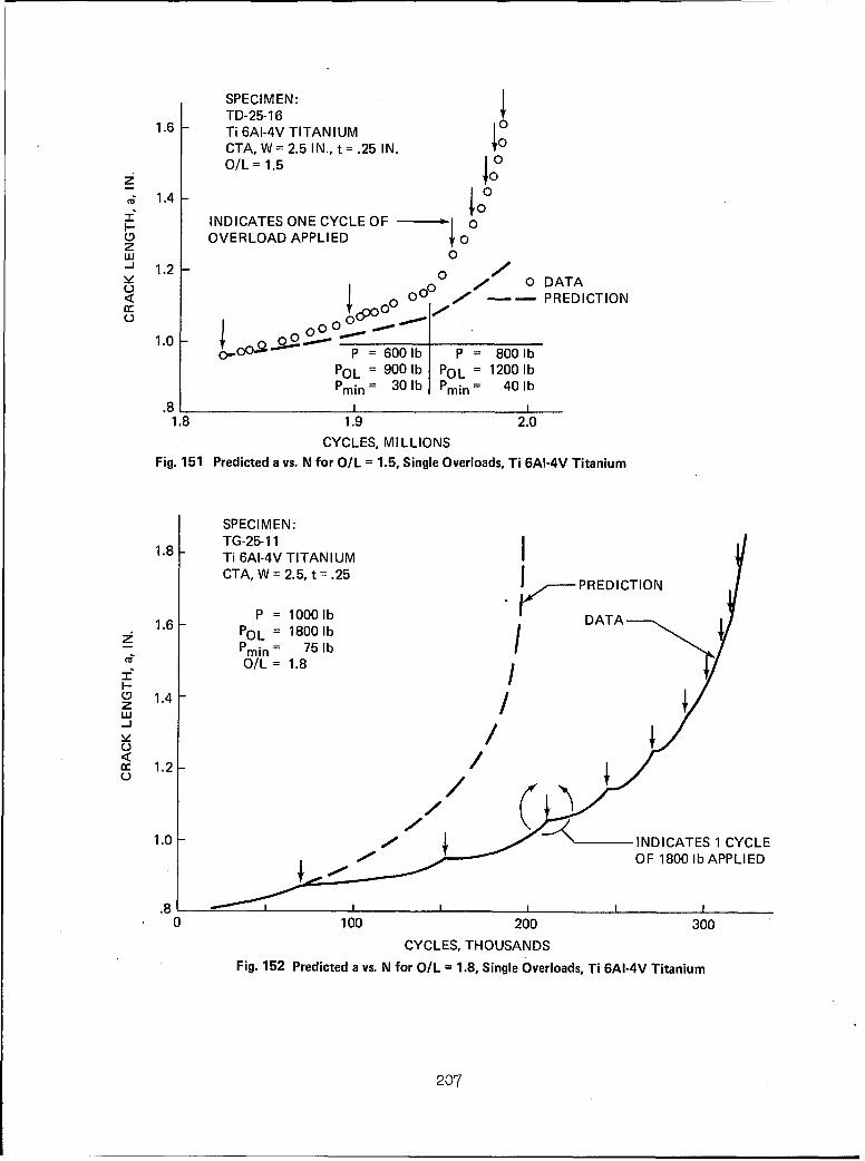
SPECIMEN:TD-25-16

1.6 Ti 6AI-4V TITANIUM 0

CTA, W = 2.5 IN., t = .25 IN.

O/L = 1.50

ci1.4 00

SINDICATES ONE CYCLE OF 0OVERLOAD APPLIED 0z

w 0"- 1.2- 0o° 0 ° oDATA

< 00- PREDICTION

0000001.0 0 0

O--oO2 P = 6001b P = 8001b

POL = 900 lb POL = 1200 IbPmin = 30 lb Pmin = 40 Ib

.8 1 _ _ _ _ _ _ _ _11.8 1.9 2.0

CYCLES, MILLIONS

Fig. 151 Predicted a vs. N for O/L = 1.5, Single Overloads, Ti 6AI-4V Titanium

SPECIMEN:

1.8 - TG-25-11Ti 6AI-4V TITANIUMCTA, W =2.5, t=.25 I~,-PREDICTION

P = 1000 lb DATA1.6 POL = 1800 lb

Pmin = 75Ib IO/L= 1.8

1.4 /-J

o= 1.2 /

1.0, INDICATES 1 CYCLE

OF 1800 Ib APPLIED

8I I

0 100 200 300

CYCLES, THOUSANDSFig. 152 Predicted a vs. N for O/L = 1.8, Single Overloads, Ti 6AI-4V Titanium

207

SPECIMEN:TD-25-2Ti 6AI-4V TITANIUM /

1.4 - C T A , W = 2 .5 IN ., t= .2 5 IN ,.N I A E O E C C E O

SP = 5501b OVERLOAD APPLIED

"¶"1.2 POL = 990 IbP 28 lb 110• "Pmin = 28I

• •

O/L = 1.8 •o

LU 0

•1.0 •< 0c 00 0 0 DATAi: --- PREDICTIONL)

.8 I I I I I III0 .1 .2 .3 .4 .5 .6 .7 .8

CYCLES, MILLIONS

Fig. 153 Predicted a vs. N for O/L = 1.8, Single Overloads, Ti 6AI-4V Titanium

SINGLE PERIODIC OVERLOAD2219-T851 ALUMINUMCTA, W = 2.5 IN., t = .25 IN.

SPECIMEN:AD-25- AD-25-26 AD-25-38

26 38 S

1.6 P (Ib) 600 500

POL (Ib) 1080 900

Pmin (Ib) 30 25

1.4-O/L = 1.8 o•l

A AN 50

1.2-- NH- AD.J A A *,A DATA

,y y••~j •• --A PREDICTION

M1.0- A AD-25-26. -.S°A A AAA----

;_..- _. --- -AD-25-38

.810 100 200 300 400

CYCLES, THOUSANDS

Fig. 154 Predicted a vs. N for O/L = 1.8, N = 500, Single Periodic Overloads, 2219-T851 Aluminum

208

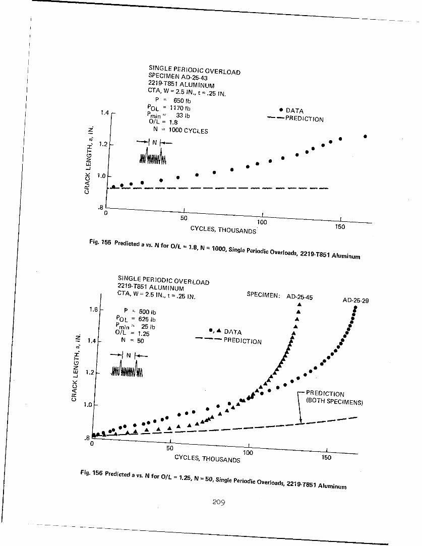
SINGLE PERIODIC OVERLOADSPECIMEN AD-25-432219-T851 ALUMINUMCTA, W = 2.5 IN., t =.25 IN.

P = 650 IbPOL = 1 1701b

0 DATA1.4 Pmin = 33 lb - PREDICTIONO/L = 1.8

N = 1000 CYCLES

ce N

S1.0 0 0c &A

8L0 501100

CYCLES, THOUSANDS 150Fig. 155 Predicted a vs. N for O/L = 1.8, N = 1000, Single Periodic Overloads, 2219-T851 Aluminum

SINGLE PERIODIC OVERLOAD2219-T851 ALUMINUMCTA, W = 2.5 IN., t = .25 IN.

SPECIMEN: AD-25-45 AD-25-29A

1.6 P = 500 Ib A 0

POL = 625 lb AP m in = 2 5 1b AD T AAO/L = 1.25 DATA A

-1.4 N = 50 - PREDICTION

N0

0

00A/K< A00

0 , *0 PREDICTION-. • ,(BOTH SPECIMENS)

1.0 - -A50

100 *A__CYCLES, THOUSANDS

150

Fig. 156 Predicted a vs. N for O/L = 1.25, N = 50, Single Periodic Overloads, 2 219-T851 Aluminum

209

SINGLE PERIODIC OVERLOADSPECIMEN AD-25-272219-T851 ALUMINUM

SP = 550 lbPOL = 688 lb

Pmin= 281bSO/L = 1.25

1.4 N = 100 CYCLES

z

1.2 -

0 0o DATA

1.0 - PREDICTION

.8 I I I I I I I0 10 20 30 40 50 60 70 80

CYCLES, THOUSANDS

Fig. 157 Predicted a vs. N for O/L = 1.25, N = 100, Single Periodic Overloads, 2219-T851 Aluminum

SINGLE PERIODIC OVERLOADTi 6AI-4V TITANIUM SPECIMEN:CTA, W = 2.5 IN., t =.25 IN. TD-25-30

_ _ _ _1 8______ TD-25- I S e

1.6 - 30 37 T23 37P (Ib) 1040 1050 TD-2D353/

z PoL(,b) 1870 1890 / / D- 2-

ea 1.4 - Pmin (Ib) 52 I / / 5N 500 500 /

I- 00I N 000,- /"- TD-25-37

1.2 ,,,nn•nr

0 0

1.0 0 o A 0 0 DATA|•0 / 0 • PREDICTION

.8 I

0 100 200 300 400

CYCLES, THOUSANDS

Fig. 158 Predicted a vs. N for O/L = 1.8, N = 500, Single Periodic Overloads, Ti 6AI-4V Titanium

210

SINGLE PERIODIC OVERLOADSPECIMEN TD-25-28Ti 6AI-4V TITANIUMCTA, W = 2.5 IN., t =.25 IN.

1.6 - P = 1040 Ib

POL = 1870 IbPmin= 52lbO/L = 1.8

z1.4 N = 1000 CYCLES

z" 1. -- N •LI--

I- / •* ~ 0o *

/cc DATA01.0 /

-- PREDICTION

.8 I0 100 200 300 400

CYCLES, THOUSANDS

Fig. 159 Predicted a vs. N for O/L = 1.8, N = 1000, Single Periodic Overloads, Ti 6AI-4V Titanium

SINGLE PERIODIC OVERLOADTi 6AI-4V TITANIUMCTA, W = 2.5 IN., t = .25 IN.

1.6-f 1P = 800lb

POL 1000 lb, /Pmin = 40 lb ,

1.4 O/L 1.25N= 50 ,/ /

z 1.2o

0o,,'. DATA SPECIMEN PREDICTION

1, _- TD-25-32 -. ..1.0, do-l- • TD-25-39

.8 II

0 100 200 300CYCLES, THOUSANDS

Fig. 160 Predicted a vs. N for O/L = 1.25, N = 50, Single Periodic Overloads, Ti 6AI-4V Titanium

211

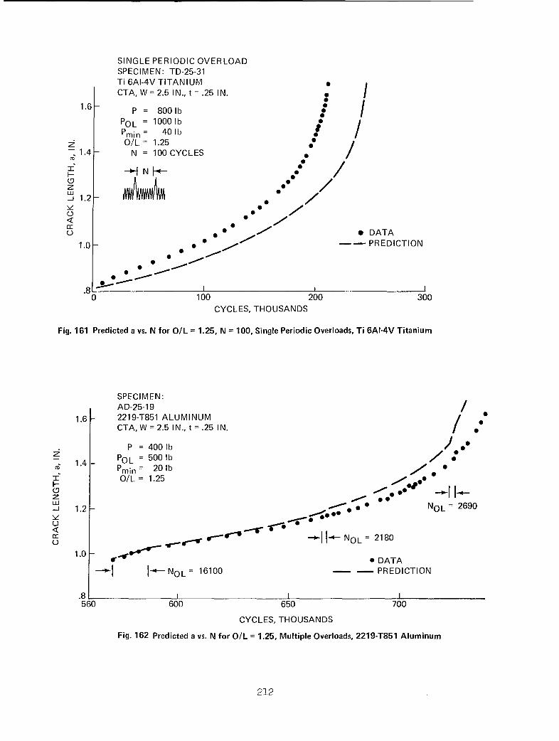
SINGLE PERIODIC OVERLOADSPECIMEN: TD-25-31Ti 6AI-4V TITANIUMCTA, W = 2.5 IN., t =.25 IN. I/ I

1.6 P = 800 Ib

POL = 1000 lbPmin = 40 Ib s

z O/L = 1.25-1.4 N = 100 CYCLES

F- S*

(J .

S1.2 * 0

<0 0

6 0 ' DATA1.0- -- PREDICTION

0

.8 -I -- :0 100 200 300

CYCLES, THOUSANDS

Fig. 161 Predicted a vs. N for O/L = 1.25, N = 100, Single Periodic Overloads, Ti 6AI-4V Titanium

SPECIMEN:AD-25-19

1.6 2219-T851 ALUMINUM /CTA, W = 2.5 IN., t =.25 IN. 0

P = 400 Ib 0 ee

- 1.4 POL = 500 IbPmin= 20 'b oS

SO/L = 1.25 1I-

z 00.j 1.2 * NOL= 2690

v g

o •.-e-''r-'- K NOL = 21801.0

0 DATA"-' -- NOL = 16100 - PREDICTION

.8 1 1

560 600 650 700

CYCLES, THOUSANDS

Fig. 162 Predicted a vs. N for O/L = 1.25, Multiple Overloads, 2219-T851 Aluminum

212

SPECIMEN:AD-25-122219-T851 ALUMINUM

1.6 CTA, W = 2.5 IN, t =.25 IN.

P = 450Ib / .:

_Z POL = 675 lb1.4 Pmin = 23 lb

O/L = 1.5 .1

- NOL 1730LU

1.2 .. rz

0 "----NOL= 880

1.0 NOL 3020 • DATAS•PREDICTION

.8 I I INI I I I

6.58 6.60 6.62 6.64

CYCLES, MILLIONS

Fig. 163 Predicted a vs. N for O/L = 1.5, Multiple Overloads, 2219-T851 Aluminum

SPECIMEN:TD-25-1 10Ti 6AI-4V TITANIUMCTA, W = 2.2 IN., t = .25 IN.

P = 900 Ib

POL = 1620 IbPmin = 45 lb DATA

1.0 O/L = 1.8 PREDICTION

I" 100I-

0 200W.8 -NOL500O

(L)

.6 i i I100 120 140 160 180

CYCLES, THOUSANDS

Fig. 164 Predicted a vs. N for O/L = 1.8, Multiple Overloads, Ti6A1-4V Titanium

213

SPECIMEN: /AD-25-24

1.6- 2219-T851 ALUMINUM /CTA, W = 2.5 IN. t =.25 IN./

'1.4- P = 6501b /3" POL = 813lb Ib- 1720%J[--OL 1720

(D Pmin = 325 lb OL;z O/L = 1.25

a- Sv 1.2-

.< •-o 1-- NoL= 3051

1.0 ,• " '"1.0

9 DATA

S-*I I-*-NoL= 4670 PREDICTION

.8 1 1 1400 450 500

CYCLES, THOUSANDS

Fig. 165 Predicted a vs. N for O/L = 1.25 and R = 0.5, Multiple Overloads 2219-T851 Aluminum

1.6- SPECIMEN:AD-25-20 6

2219-T851 ALUMINUMCTA, W = 2.5 IN., t =.25 IN.

_ 1.4 -C6 P = 7001b

POL = 1050Ib NOL = 640HPmin = 3501b

Z 1.2- O/L = 1.5

r 4 [NOL= 1010

o1.0- ••• '

- * DATA

* * -•F--NOL= 1550 PREDICTION

.8

250 300 350

CYCLES, THOUSANDS

Fig. 166 Predicted a vs. N for O/L = 1.5 and R = 0.5, Multiple Overloads 2219-T851 Aluminum

214

1.6-

SPECIMEN: 2

TD-25-23Ti 6AI-4V TITANIUM

1.4 CTA, W= 2.5 IN, t=.25 IN. /_z P = 12001b / /

POL = 1500 Ib (*.

Pmin = 600 Ib __1 - 1590

O/L = 1.25

[.--NOL 1930

< 1.0

"". --JNOL= 1590 • DATA.8---PREDICTION

0 100 200 300CYCLES, THOUSANDS

Fig. 167 Predicted a vs. N for O/L = 1.25 and R = 0.5, Multiple Overloads, Titanium

SPECIMEN:TD-25-21Ti 6AI-4V TITANIUM

1.4 CTA, W = 2.5 IN., t =.25 IN.

P = 1200lb ,"

POL = 1800 Ib

1.2 Pmin = 600 lb . 738O/L = 1.5z -:. -----

- -

e 1.0 - -U ~ .J *DATA

-4-1I-4-NOL= 530 -- PREDICTION

.8I I I l I I I I0 10 20 30 40 50 60 70 80

CYCLES, THOUSANDS

Fig. 168 Predicted a vs. N for O/L = 1.5 and R = 0.5, Multiple Overloads, Titanium

215

["NOL

SPECIMEN: P

AD-25-107 E i:ikLZ2219-T851 ALUMINUMCTA, W 2.5 IN., t =.25 IN. .NS

1.12 -NOL= 10 0/

P = 650 lb

/ POL = 1170lb- Pmin = 32 lb

::c oO/L = 1.8I-

z 1.10

v ODATA0<• • PREDICTION

C-)

1.08 I I I0 4 8 12 16

A NS, THOUSANDS

Fig. 169 Predicted a vs. A Ns for O/L = 1.8 and NOL 10, 2219-T851 Aluminum

1.20-NOL= 100 /

SPECIMEN: /

AD-25-1092219-T851 ALUMINUM

C- 1.18 CTA, W = 2.5 IN., t= .25 IN.

I-: •DATAI- -- PREDICTION

V

"o P = 550 lbr<y 1.16- POL = 825 lb

Pmin 28 IbO/L = 1.5

1.14 I I0 2 4 6 8

A NS, THOUSANDS

Fig. 170 Predicted a vs. A Ns for O/L = 1.5 and NOL 10, 2219-T851 Aluminum

216

SPECIMEN:AD-25-110 0 DATA2219-T851 ALUMINUM PREDICTIONCTA, W = 2.5 IN., t =.25 IN.

1.04 -

NOL= 2

1.02 -

00

1.-00 NO L

(UL(

z .98 ANSF NOL 5 40

C-)P = ~ ~ 650 lb< I OL =1170 lb

o .96. Pmin = 32 lbOIL-= 1.8

.94 NO= 100

.92 0

S•oo - -" - - 1I"-No

.90I102 4 6 8 10 12

A"Ns THOUSANDS

Fig. 171 Predicted a vs. A Ns for OL = 1.8 and NOL = 2,O5 & 10, 2219-T851 Aluminum

217

SPECIMEN:TD-25-1 10Ti 6AI-4VCTA, W = 2.20, t = .251

P = 900 lb

1.4 POL = 1620 lbPmin = 45 lbO/L = 1.8

z LOAD (Ib) .*NOLI 20

3" 16201 DATA-F- 2(9 900-LU J

-j 1.0- 55• ~CYCLES10

<00

N200.8 - N LPREDICTION

S....--• • -NOL< Nsat

.6 I

100 150 200 250

CYCLES, THOUSANDS

Fig. 172 Predicted a vs. N for O/L = 1.8 and NOL < Nsat, Ti 6AI-4V Titanium

SPECIMEN:TD-25-111Ti 6AI-4VCTA, W = 2.194, t = .250

P = 900 lb

POL = 1620 lbPmin = 45 lb

z LOAD (Ib) H-NoLS1.3 A 2000

- 1620 PREDICTION

S20 0 0-j 1.1 9005 200 50SCYCLES 100

cc: 50C' 20 L / "\ ..

.9 10 20 DATA

NOL 2 5•INOL= . NOL < Nsat

.7 - ' I- .60 80 100 120 140 160 180 200 220

CYCLES, THOUSANDS

Fig. 173 Predicted a vs. N for O/L = 1.8 and NOL < Nsat, Ti 6AI-4V Titanium

218

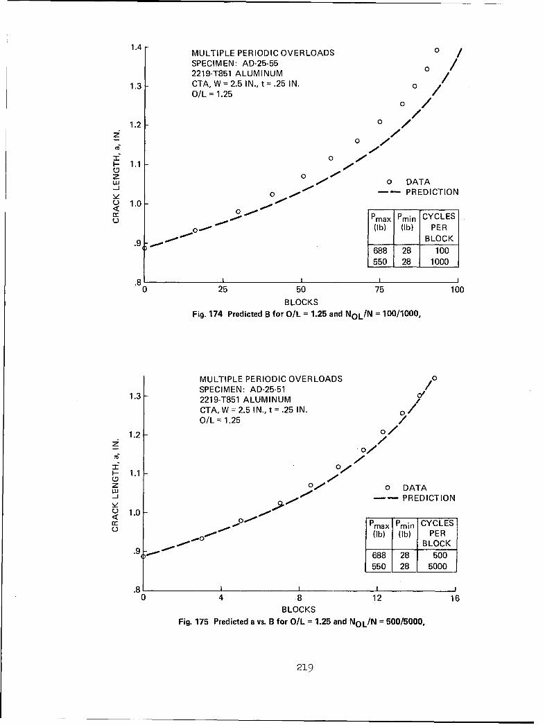
1.4 MULTIPLE PERIODIC OVERLOADS 0

SPECIMEN: AD-25-55 /2219-T851 ALUMINUM /

1.3 CTA, W = 2.5 IN., t =.25 IN. oO/L= 1.25

/

1.2 0 /

-0 -

I-- 1.1 -

0u 0 DATA

So - -- PREDICTION1.0 o__

Pmax Pmin CYCLESo (Ib) (Ib) PER

.9 BLOCK688 128 100

550 28 1000

.8 I L L j

0 25 50 75 100

BLOCKS

Fig. 174 Predicted B for O/L = 1.25 and NoL/N = 100/1000,

MULTIPLE PERIODIC OVERLOADS 0SPECIMEN: AD-25-51 /o

1.3 2219-T851 ALUMINUM 0

CTA, W= 2.5 IN., t= .25 IN. 0/O/L= 1.25 /

1.2 0/

-- 1 .1

z 0" 0 DATAU. /-- PREDICTION

19.o1.0 o/<cc Pmax Pmin CYCLES

(Ib) (Ib) PERBLOCK

688 28 500550 28 5000

.8 L0 4 8 12 16

BLOCKSFig. 175 Predicted a vs. B for O/L = 1.25 and NOL/N = 500/5000,

219

1.4 MULTIPLE PERIODIC OVERLOADSSPECIMEN: AD-25-472219-T851 ALUMINUM

CTA, W = 2.5 IN., t =.25 IN.

1.3 O/L = 1.25

/0R=0.5/

z1.2-//

/0

z 1.1 70 DATA-J 7 PREDICTION

"lo

S1.0 max CYCLES

S(Ib) (lb) PER_ _ _ BLOCK

688 275 200

550 275 1000

.8 I I I I I I

0 40 80 120 160 200 240 280 320

BLOCKS

Fig. 176 Predicted a vs. B for O/L = 1.25 and NOL/N = 200/1000, R = 0.5,

Multiple Periodic Overloads, 2219-T851 Aluminum

MULTIPLE PERIODIC OVERLOADS /1.3- SPECIMEN: AD-25-53

2219-T851 ALUMINUMCTA, W = 2.5 IN., t =.25 IN.

O/L = 1.25R 0.5 A;• 1.21

F-

.1 ,0 DATA

7'- PREDICTION

0

Pmax Pmin CYCLESI 0b) (Ib) PER

/ BLOCK

.9 F/ 1031 413 1000

825 413 5000

"08 4 8 12 16

BLOCKSFig. 177 Predicted a vs. B for O/L = 1.25 and NOL/N = 1000/5000, R = 0.5,

Multiple Periodic Overloads, 2219-T851 Aluminum

220

1.4 MULTIPLE PERIODIC OVERLOADS

SPECIMEN: AD-25-57 02219-T851 ALUMINUMCTA, W = 2.5 IN., t = .25 IN. 0

1.3 O/L =1.5 /0/

S1.2O

o o /

00z'" -"-J 1.1 O0 •o a-

C< 00 DATA

0 PREDICTION

0 a- Pmax Pmin CYCLES(Ib) (Ib) PER

.9- _ _"BLOCK

.9 825 28 100550 28 500

.8 I I I I I I0 20 40 60 80 100 120 140 160

BLOCKSFig. 178 Predicted a vs. B for O/L = 1.5 and NOL/N = 100/500, Multiple Periodic Overloads,

2219-T851 Aluminum1.3 / 0

/MULTIPLE PERIODIC OVERLOADS 0 0SPECIMEN: AD-25-59 /

z; 1.2 2219-T851 ALUMINUM 0-- CTA, W = 2.5 IN., t = .25 IN.

arO/L 1.5 0

I- -0z 1.1w -

S0 ODATAo .0- PREDICTION

O 1.0 P Pmax Pmin CYCLES

S(Ib) (Ib) PER

__ _ _ BLOCK0 825 28 200

09 - 550 28 1000

.8 I I I I I I I

0 10 20 30 40 50 60 70 80 90

BLOCKSFig. 179 Predicted a vs. B for O/L = 1.5 and NoL/N 200/1000, Multiple Periodic Overloads,

2219-T851 Aluminum

221

1.4 MULTIPLE PERIODIC OVERLOADSSPECIMEN: AD-25-342219-T851 ALUMINUMCTA, W = 2.5 IN., t = .25 IN.

1.3 O/L =1.5 /7

70

S1.2 -

S-4-

A * DATAz 1.1uz 11- PREDICTION

cc

-J 0-

0 1.0 -1Pmax Pmin CYCLES

(Ib) (Ib) PERBLOCK

825 28 100550 28 1000

.8II1 I I I I10 10 20 30 40 50 60 70 80

BLOCKS

Fig. 180 Predicted a vs. B for O/L = 1.5 and NOL/N = 100/1000,

Pmax Pmin CYCLES SPECIMEN:(Ib) (Ib) PER TD-25-54

BLOCK Ti 6AI-4V TITANIUM

1350 45 50 CTA, W = 2.5 IN., t =.25 IN.-_ 900 45 500 O/L 1.5

i1.2 DATA0z

PREDICTIONo 1.0

.8'0 100 200 300

BLOCKS

Fig. 181 Predicted a vs. B for O/L = 1.5 and NOL/N = 50/500,

222

SPECIMEN:TD-25-50Ti 6AI-4V TITANIUM

-Pmax -mi~mn CYCLES CTA, W = 2.5 IN., t =.25 IN.~max min CCLESOIL = 1.5(Ib) (Ib) PER

BLOCK

1.4 1350 45 100900 45 1000

•. 1.2 S~DATAQI.-

zLJ

v 1.0o

ccN PREDICTION

.8 . I I I I I II

0 20 40 60 80 100 120 140 160

BLOCKS

Fig. 182 Predicted a vs. B for O/L = 1.5 and NOL/N = 100/1000, Multiple Periodic Overloads, Ti 6AI-4V Titanium

SPECIMEN:

TD-25-52Ti 6AI-4V TITANIUMCTA, W = 2.5 IN., t= .25 IN.

Pmax Pmin CYCLES O/L 1.5(lib) 0ib) PER

BLOCK

z 1.4 1350 45 200- 900 45 1000

z 1.2DII •zu PREDICTION

C-)<• •• DATA

o 1.0

.8 I I I I I I

0 20 40 60 80 100 120 140

BLOCKS

Fig. 183 Predicted a vs. B for O/L 1.5 and NOL/N = 200/1000, Multiple Periodic Overloads, Ti 6AI-4V Titanium

223

SPECIMEN:TD-25-46Ti 6AI-4V TITANIUMCTA, W = 2.5 IN., t =.25 IN.O/L = 1.25

Pmax Pmin CYCLES(Ib) (Ib) PER

BLOCK1125 45 100900 45 1000

1.4-

'" 1.2- DATA

zLU-J

v 1.0- -i

~- - - --cc- PREDICTION.

.8 ---- I I I I

0 10 20 30 40 50 60 70 80 90BLOCKS

Fig. 184 Predicted a vs. B for O/L = 1.25 and NOL/N = 100/1000, Multiple Periodic Overloads,Ti 6AI-4V Titanium

SPECIMEN:TD-25-56Ti 6AI-4V TITANIUMCTA, W = 2.5 IN., t .25 IN.O/L = 1.25

Pmax Pmin CYCLES1.4- (Ib) (Ib) PER DATA

clý 1125 45 500

3" 900 45 50001.2-

<10

w PREDICTION

C-V

.8 • ' II IIII I0 10 12 14 16 18 20 22 24BLOCKS

Fig. 185 Predicted a vs. B for O/L = 1.25 and NOL/N = 500/5000, Multiple Periodic Overloads,Ti 6AI-4V Titanium

224

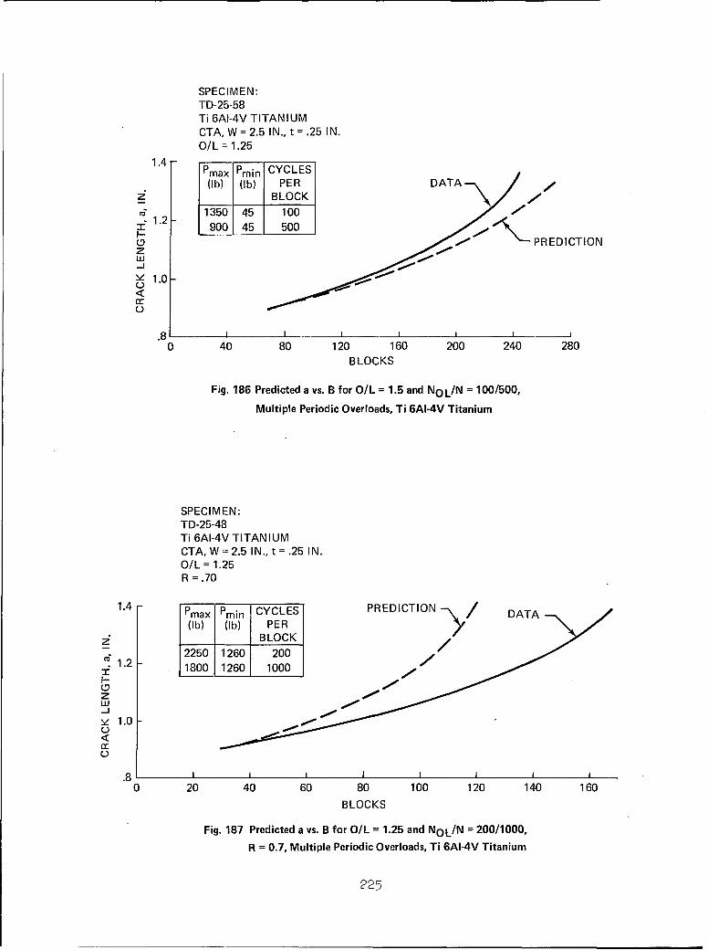
SPECIMEN:TD-25-58Ti 6AI-4V TITANIUMCTA, W = 2.5 IN., t = .25 IN.O/L = 1.25

1.4 Pmax Pmin CYCLES

(Ib) (Ib) PER DATA ,eZ; BLOCK

S1.2 1350 45 100: 900 45 500

PREDICTIONzw-J

1.0

.8 I I0 40 80 120 160 200 240 280

BLOCKS

Fig. 186 Predicted a vs. B for O/L = 1.5 and NOL/N = 100/500,

Multiple Periodic Overloads, Ti 6AI-4V Titanium

SPECIMEN:TD-25-48Ti 6AI-4V TITANIUMCTA, W = 2.5 IN., t = .25 IN.O/L = 1.25R = .70

1.4 Pmax Pmin CYCLES PREDICTION DATA

(ib) (ib) PERBLOCK

2250 1260 2003 1.2 1800 1260 1000

z --J

1.0

.8 I IIII II

0 20 40 60 80 100 120 140 160

BLOCKS

Fig. 187 Predicted a vs. B for O/L = 1.25 and NOL/N = 200/1000,

R = 0.7, Multiple Periodic Overloads, Ti 6AI-4V Titanium

225

BLOCK LOADING - HIGH-LOW2219-T851 ALUMINUM SPECIMENCTB, W =2.5 IN., t =.25 IN. / AG-25-06

1.4 - Pmax Pmin CYCLES

(Ib) (Ib) PER-Z BLOCK

C6 750 25 1000

Z 500 25 3000zLU-J

o 1.0 •rr DATA

PREDICTION

.8

0 10 20 30

BLOCKS

Fig. 188 Predicted a vs. B for High-Low Block Loading, 2219-T851 Aluminum

BLOCK LOADING - LOW-HIGH2219-T851 ALUMINUM

1.6 CTB, W= 2.5 IN., t =.25 IN. 0 AG-25-09

Pmax Pmin CYCLES / 01.4 (Ib) (Ib) PER I SPECIMEN: 0

50 BLOCK AG-25-08 o 0650 25 3000 0

625 25 2000 t O

1.2- 750 25 1000 0/

LU-J / g0

10 / 00

0 00o< 1.0- 0

0 0 0 DATA0 000

. O8 00 PREDICTION

.8 f 0"

0 20 40 60BLOCKS

Fig. 189 Predicted a vs. B for Low-High Block Loading, 2219-T851 Aluminum

226

BLOCK LOADING - RANDOM2219-T851 ALUMINUM SPECIMEN:CTB, W = 2.5 IN., t = .25 IN. AG-25-04 AG-25-05

1.6 Pmax Pmin CYCLES* 0

(Ib) (Ib) PER____ ____ BLOCK 0, /

1A4 750 25 100625 25 200 0 /

S500 25 300 /1.2J *RANDOMIZED /v 1.2 El

1.0 00 , 0/ /

1.0

0 6,0 DATA0 -r PREDICTION

0 100 200 300

BLOCKS

Fig. 190 Predicted a vs. B for Block Random Loading, 2219-T851 Aluminum

BLOCK LOADING -2219-T851 ALUMINUMCTB, W 2.5 IN., t = .25 IN.

AG-25 Pmax Pmin CYCLES SEQUENCE(Ib) (Ib) PER

1.6 BLOCK1250 500 1000

-22 1125 500 2000 HIGH

1000 500 3000 LOW AG-25231.4 1000 500 3000 /

-23 1125 500 2000 LOW

S1250 500 1000 HIGH /(D 1.2 DATASSPECIMEN: 0 DAW AG-25-22 / •, 0 AG-25-22

•,,e E0 AG-25-23(SOLID SYMBOLS

cc 1.0 5 INDICATE WHERELOAD WAS REDUCEDTO ZERO)

i- - PREDICTION".8 '• i ~ EXCLUDING ZERO

LOAD EXCURSIONS

0 4 8 12 16

BLOCKS

Fig. 191 Predicted a vs. B for High-Low and Low-High Block Loading, Rmin = 0.5, 2219-T851 Aluminum

227

BLOCK LOADING - RANDOM2219-T851 ALUMINUMCTB, W = 2.5 IN., t =.25 IN.

1.6 Pmax Pmm CYCLES* AG-25-28 AG-25-24

(Ib) (Ib) PER 0 0 0

BLOCK I01250 500 100 0

1.4 1125 500 200 /01000 500 300 E

I01.2 *RANDOMIZED /

, 00 DATA2

(SOLID SYMBOLSo -INDICATE WHERE

.1. LOAD WAS REDUCEDo 1.0 N TO ZERO)

0 , -•. O PREDICTION,0 o EXCLUDING ZERO

.8] 0 LOAD EXCURSIONS

0 20 40 60 80 100 120 140B LOCKS

Fig. 192 Predicted a vs. B for Block Random Loading, Rmin =0.5, 2219-T851 Aluminum

BLOCK LOADING - LOW-HIGH, 4 LEVELS2219-T851 ALUMINUM

1.6 CTB, W= 2.5 IN., t =.25 IN.

Pmax Pmin CYCLES(Ib) (Ib) PER AG-25-25

BLOCK 0z 1.4 500 25 3000 /""6 625 25 2000 /0S750 25 1000 / 0F- 1000 25 1 0D I/2! 1.2 0-J /0

/ 0

-•1.0 0 0 0 DATA0 PREDICTIONSo0

0 0

0 20 40 60

BLOCKS

Fig. 193 Predicted a vs. B for 4 Level Low-High Block Loading, 2219-T851 Aluminum

228

BLOCK LOADING - LOW-HIGHTi 6AI-4V TITANIUMCTB, W= 2.5 IN., t =.25 IN.

SPECIMEN:

"Pmax Pmin CYCLES

S (Ib) (Ib) PERBLOCK

1.4 - 500 25 3000 0

z/ 625 25 2000

750 25 1000

S1.2 IzUJ-

o !

c10 / 00• / DATA

- - PREDICTION

0 200 400 600BLOCKS

Fig. 194 Predicted a vs. B for Low-High Block Loading, Ti 6AI-4V Titanium

BLOCK LOADING - LOW-HIGHTi 6AI-4V TITANIUM (b) (min CYLESCTB, W= 2.5 IN., t =.25 IN. (Ib) (Ib) PERCT=W__________ BLOCK

800 40 30001000 40 2000

1.6- 1200 40 1000 e SPECIMEN:1 1 TG-25-09

I 0

.1.4 /

1.2 -z /

51.0 7 0 0 DATAS -- PREDICTION

4.8"80 20 40 60 80

BLOCKS

Fig. 195 Predicted a vs. B for Low-High Block Loading, Ti 6AI-4V Titanium

229

BLOCK LOADING - HIGH-LOWTi 6AI-4V TITANIUMCTB, W = 2.5 IN,, t =.25 IN.

SPECIMEN: TG-25-08 TG-25-07

1.5Pmax Pmin CYCLES 0

(Ib) (Ib) PERBLOCK /

1200 40 1000 01.3 1000 40 2000 /

800 40 3000 / 0

u" / [-6

( 0

j 0 0

C- .9 ",

0,0 DATA-- PREDICTION

7)I I I I I I

0 10 20 30 40 50 60 70 80BLOCKS

Fig. 196 Predicted a vs. B for High-Low Block Loading, Ti 6AI-4V Titanium

BLOCK LOADING - RANDOM SPECIMEN: TG-25-05 TG-25-04

Ti 6AI-4V TITANIUM 0l 0CTB, W = 2.5 IN., t =.25 IN.

1.6 E0Pmax Pmin CYCLES* 0(Ib) (Ib) PER

__B __ LOCK 01.4 1200 120 300 /

_ 1000 100 200 0800 8 0 /

*RANDOMIZED 0 /

Z 1.2 0 0

01.0 0 E

C'1.0 0"

0,0E1 DATA--- PREDICTION

.80 100 200 300 400

BLOCKS

Fig. 197 Predicted a vs. B for Block Random Loading, Ti 6AI-4V Titanium

230

BLOCK LOADINGTi 6AI-4V TITANIUM SPECIMEN:

1.6 CTB, W 2.5 IN., t = .25 IN. TG-25-22

TG-25 Pmax Pmin CYCLES(Ib) (Ib) PER 0

BLOCK1600 400 1000

1.4 -21 1400 400 2000 Tz 1200 400 3000 / 0TG-25-21 O

1e 200 400 3000-22 1400 400 200 DATA

" 1.2 -1600 400 1000 0 0 TG-25-21"z0 [] TG-25-22

00 (SOLID SYMBOLSo INDICATE WHERE< 1.0 -.AJK# 0 LOAD WAS REDUCED

CC 0U 0 TO ZERO)

000 -- PREDICTION,.8 .1- OEXCLUDING ZERO

0 0 • •OLOAD EXCURSIONS

0 10 20 30BLOCKS

Fig. 198 Predicted a vs. B for High-Low and Low-High Block Loading,Rmin = 0.333, Ti 6AI-4V Titanium

BLOCK LOADING - RANDOMTi 6AI-4V TITANIUM 0

1.6 CTB, W = 2.5 IN., t =.25 IN. SPECIMEN:

Pmax Pmin CYCLES* TG-25-23 0(Ib) (Ib) PER(1) 0 ) BLOCK ]

1.4 1600 400 100 0/

S1400 400 2001200 400 300 0/

1.2 *RANDOMIZED 0*1.120 0

z DATA,,0 0 (SOLID SYMBOLS

000 O INDICATE WHERE< 1.0 .0 LOAD WAS REDUCED

0 TO ZERO)

0-- PREDICTION,

.8 EXCLUDING ZEROLOAD EXCURSIONS

0 100 200 300

BLOCKS

Fig. 199 Predicted a vs. B for Block Random Loading, Rmin = 0.333, Ti 6AI-4V Titanium

231

BLOCK LOADING - 4 LEVELTi 6AI-4V TITANIUM

CTB, W = 2.5 IN., t = .25 IN.

TG-25 Pmax Pmin CYCLES

(Ib) (Ib) PERBLOCK

800 40 3000-19a 1000 40 2000

1200 40 10001600 40 1

1600 40 1-18 1200 40 1000

1000 40 2000

800 40 3000 o

SPECIMEN: I I "°

z 1.4 TG-25-18 //TG-25-19A 00

(D 1.2 -•z/ 00 O

o 1.0- DATAC c TG-25-19a

So o 0 0 TG-25-18

.8 e.0 €) 0 * 3 0 --P PREDICTION

II I I0 20 40 60 80

BLOCKS,

Fig. 200 Predicted a vs. B for High-Low and Low-High 4 Level Block Loading, Ti 6AI-4V Titanium

1.0- BLOCK LOADING - FIGHTER SPECTRUM

2219-T851 ALUMINUMCCP, W = 6.01 IN., t =.251 IN. 6

.9 - SPECIMEN: S

AG-25-15p

C6 0

S.8 -•8 64 LEVELS

z PER BLOCK-j

- .7 . 66 LEVELS0 0 PER BLOCKCr

.6.00 0DATA

-PREDICTION

0 10 20 30

BLOCKS

Fig. 201 Predicted a vs. B for Fighter Spectrum, 2219-T851 Aluminum

232

1.0- BLOCK LOADING - FIGHTER SPECTRUMTi 6AI-4V TITANIUMCCP, W = 6.01 IN., t = .284 IN.SPECIMEN:TG-25-3P /LVL

64 LEVELS 66/ "PEPERLBLOCK

PER BLOCK/ /

° ///.- I

,I,w ,/C).7 -

• DATA

.6 / .".PREDICTION

.5 I I I I I I250 270 290 310

BLOCKS

Fig. 202 Predicted a vs. B for Fighter Spectrum, Ti 6AI-4V Titanium

6.SPECIMEN: 4.i5'2.0- SPECIMEN: CONSTANT AMPLITUDE I4.52219-T851 ALUMINUM 6 ksi, R =-1CCP, W = 6.0 IN., t= .25 IN.

1.5

S 6ksi 4.5Smin = .3 ksi 3.

1 INDICATES (1)CYCLE DATA /4 6.45

OF COMPRESSIONLOAD APPLIED. VALUE 1.5SHOWN IS MAGNITUDE 6.

,z, 10_INKSI . 5.-1 1.5 ? 1 L T •_.•L 4.5 6.'• -•,CONSTANT AMPLITUDE

CC 1 5 3. •o {•='' S = 6 ksi, R =.05

"" •- PREDICTION.5

0[0 550 600 650 700

CYCLES, THOUSANDS

Fig. 203 Predicted a vs. N for Occasional Compression Loads, 2219-T851 Aluminum

233

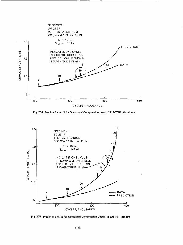
SPECIMEN:AG-25-9P2219-T851 ALUMINUM

CCP, W = 6.0 IN., t =.25 IN.

2.0 S = 10 ksiSmin = 0.5 ksi

PREDICTION

Z INDICATES ONE CYCLESOF COMPRESSION LOAD

3' 1.5 APPLIED. VALUE SHOWNH- IS MAGNITUDE IN ksi

z DATAwu15

0< 1.0 10

.5

480 490 500 510

CYCLES, THOUSANDS

Fig. 204 Predicted a vs. N for Occasional Compression Loads, 2219-T851 Aluminum

2.5

SPECIMEN: 20

TG-25-1 PTi 6AI-4V TITANIUMCCP, W = 6.0 IN., t = .25 IN.

10

2.0 S = 10 ksi

Smin = 0.5 ksi

SINDICATES

ONE CYCLE 20

OF COMPRESSION STRESS(-Z 1.5 APPLIED. VALUE SHOWNJ IS MAGNITUDE IN ksi 10

5,;r-,

m0

1.0 20

5• •I " DATA

-- PREDICTION.5

200 300 400

CYCLES, THOUSANDS

Fig. 205 Predicted a vs. N for Occasional Compression Loads, Ti 6AI-4V Titanium

234

R FORCOMPRESSIONSPIKE:

2.5 SPECIMEN:TG-25-1 P

Ti 6AI-4V TITANI UM1 CCP, W = 6. IN., t =.25 IN.

2.0 S = 10ksiz Y -.5 Smin = .5 ksi

" 1-2I--

z. 1.5 DATA

w .5J - CONSTANT AMPLITUDE

v -1 CALCULATION FORSS= 10 ksi, R =.05

U-.- 1.0 .

* * *-2* ..

.5 -5

0 10 20 30 40 50 60 70

ANs, THOUSANDS

Fig. 206 Data vs. Constant Amplitude Growth after Occasional Compression Loads, Ti 6AI-4V Titanium

-18, +91

1.8 S = 6 ksi SPECIMEN:1min = 0.3 ksi AG-25-10P +9, -18

2219-T851 ALUMINUM

1.6 CCP, W = 6.0 IN., t =.25 IN. +9,-12 /.

TENSILE OVERLOAD FOLLOWED BY /eA COMPRESSION SPIKE 1/6

S1.4 - 9 .+12.6, -18 A;cc 6

C 1.2 , +12.6, -12z TIME

S1n c1+12.6, -3 e• ./1.0 -12 . TYP.+9,-.12 +9 -80i e.D T

+96 - ***~- PREDICTION+9,+9 -13..86 -12 *DAT

500 550 600 650 700 750

CYCLES, THOUSANDS

Fig. 207 Predicted a vs. N for Tension/Compression Spike Sequences, 2219-T851 Aluminum

235

SPECIMEN:AD-25-1152219-T851 ALUMINUMCTA, W = 2.5 IN., t =.25 IN.

1.6- P = 800 Ib

Pmin = 400 Ib

POL = 0,1200 Ib /

1.4 1200• /

±1 800 / , '2 12!0 TIMEUj 0

_j _

o< 1.0-1.0 TYP. D ATA

o • DATA

V. " - PREDICTION.80.•.-W- "

50 100 150 200CYCLES, THOUSANDS

Fig. 208 Predicted a vs. N for Underload/Overload Spike Sequence, 2219-T851 Aluminum

SPECIMEN:AD-25-116

2219-T851 ALUMINUMCTA, W = 2.5 IN., t = .25 IN.

1.6 P = 800 IbPmin = 400 Ib

POL = 1200, 0 Ib

S1.4 1200 NOL / 1

108 00

z 0,, 1.2 -J 400 ee

0 0 1, 10

0 o DATA.8 -oPREDICTION

100 150 200

CYCLES, THOUSANDS

Fig. 209 Predicted a vs. N for Overload/Underload Spike Sequences, 2219-T851 Aluminum

236

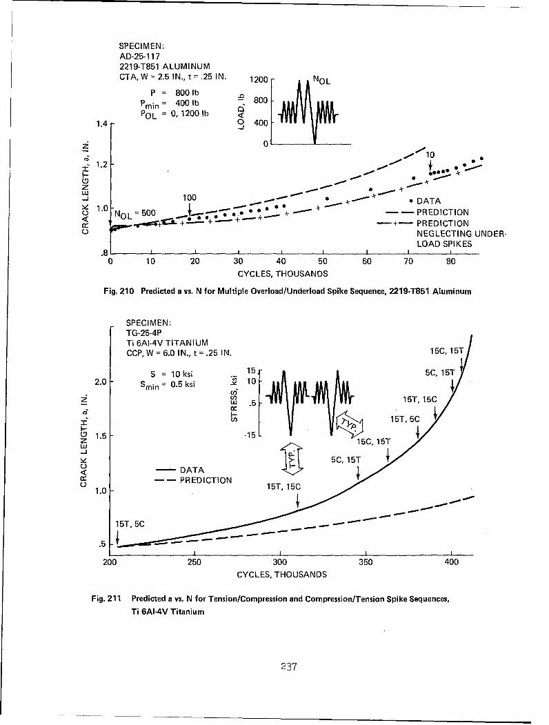
SPECIMEN:AD-25-1172219-T851 ALUMINUMCTA, W = 2.5 IN., t =.25 IN. 12008- NOL

~min = 400 I80lb -800 -POL =0, 1200 lb

1.4 9 400-

1.0~ ~ NOL 50 0001RD~lS1.2 fee -

10 +ATAS1.0 _•.-NIoL-500 •""' -"+ PREDICTION

S••,.•, i+'•- ... +... --- • - - PREDICTION

-U NEGLECTING UNDER-

LOAD SPIKES.8 I

0 10 20 30 40 50 60 70 80

CYCLES, THOUSANDS

Fig. 210 Predicted a vs. N for Multiple Overload/Underload Spike Sequence, 2219-T851 Aluminum

SPECIMEN:TG-25-4PTi 6AI-4V TITANIUMCCP, W = 6.0 IN., t =.25 IN. 15C, 15T

15,-S = 10 ksi 15 5C, 15T

2.0 Smin =0.5 ksi 10

U,-w .5 15T, 15C

3ý 15T, 5CS-15 _ 15C, 15T

v 5C, 15T- DATA ,OSl"

1015T, 15C •

15T, 5C

CYLSTOUAD

200 250 300 350 400

CYCLES, THOUSANDS

Fig. 211 Predicted a vs. N for Tension/Compression and Compression/Tension Spike Sequences,

Ti 6AI-4V Titanium

237

SPECIMEN:TD-25-119Ti 6AI-4V TITANIUM

2100

1.2 1400-

S700-- PECI

1.0 0

'1"D-25-11

Uj '

< .8 .cc F DATA

Ti6A4 IT-PREDICTION160 170 180 190 200 210 220 230 240

CYCLES, THOUSANDS

Fig. 212 Predicted a vs. N for Overload/Underload Spike Sequences, Ti 6A1-4V Titanium

SPECIMEN:TD-25- 118Ti 6AI-4V TITANIUMCTA, W = 2.2 IN., t = .25 IN.

1.2 2100,

6 Q1400I0

"- 0 0( o 1.0- _- 700 Pz

w0

L)00 0.

00 o *DATA0 -- PPREDICTION

.6 1 1 1 1 I 1 1 I I

80 90 100 110 120 130 140 150 160

CYCLES, THOUSANDS

Fig. 213 Predicted a vs. N for Underload/Overload Spike Sequences, Ti 6AI-4V Titanium

238

SPECIMEN:TD-25-117Ti 6AI-4V TITANIUMCTA, W = 2.2 IN., t = .25 IN.

2100. -40 NOL

-- 1400 . A,,,

1.2- 00-

"1.0z •0

NOL500

< .8 - • DATAPREDICTION

.6 1 i i

20 30 40 50 60 70 80 90 100

CYCLES, THOUSANDS

Fig. 214 Predicted a vs. N for Multiple Overload/Underload Spike Sequences, Ti 6AI-4V Titanium

239

DECREASIN CLOSURE CONDTIOScOELACNDTN

'~ef=S(max)-S

C Kf= f (R)fx~a

da2 = da/d(maxKf)

aMaNIMda

Fig. 15Ov Ral EogcFlwChr

ADJSTEN

INITIAL CONDITIONS S(max) OL' Scl

ROL, aOL, P

MINIMUM STRESS ADJUSTMENT

•~YES

ROL = S(min)/S(max)OL

Cf' = Cf (ROL)'

Sc 1 = Cf x S(max) OL

aOL = a

DECREASING CLOSURESSc =Sc21

ISc = sc (A a)

OVERLOAD CONDITION J YES Sc Sc2

÷~NOI y + ' (J)

Sc =-") S(max)

UPDATE CONDITIONS YES

••~NO

S~a) Smx YES

NO RESET CONDITIONS

RESET CONDITIONS Scl = Sc2

S(max) OL = S(max)

ROL= R

aOL = a

p = p (S(max))

Fig. 216 Detail Logic Flow

241

t ~S

/ \ /Sr

Sr

0 ry ao

a) a

S t 2 SI ta0 0 / \ ,

S /S

a

b) d)

Fig. 217 Residual Stress Distributions

242

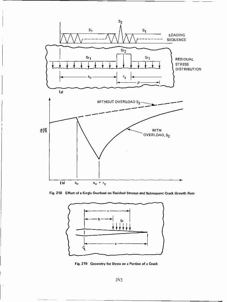
S2

Si S1LOADING

S--------- SEQUENCE

_______Sr______________ RESIDUAL

DISTRIBUTION

(a)

WITHOUT OVERLOAD 82 -

cmZ-•I-oZ-. WITH/ OVERLOAD, S2

(b) ao ao + ry

Fig. 218 Effect of a Single Overload on Residual Stresses and Subsequent Crack Growth Rate

C

Fig. 219 Geometry for Stress on a Portion of a Crack

243

10- NO

LU

CU0

LU1 A

< 1-

03.

cc0.UvC-,

1 OL

Fig.~ ~ > 22 esda FrePrdctosvsDt

2n 15 J

4 0I- 0 L

0 0 0 2

0 x 0<00< < J(

0H _3 <~4 i C~i.U- . D Z CUL

coo

~zCU'

cc4

*U-_w

NCN

CC?o 0

)~3O~fPNILP- '31VU HIMOýJD )OVUOep

LO

LUU0mZ -j

0 0 * -

0LU WU 0I

4U4

CLC

~~A!)1)9NV LO

0o Lo 0C.ý - _j

UU-

0 0L

00o *iZ

~13A~NI ~ 'IV~JH1M~J9 O-a-0 2

245c

X cc0 - C'l) (D 0 CD) 0LO ~- N O

0

-0)

C.,D

W 0 X

C: E,

E c_ 0 c

0

00 0Q0, - cv

CL

0

L/3 0

c-J

00

0 00

CN C)

'N 'L UD3 NV O:-V

2460

TABLE 1 CONSTANT AMPLITUDE TEST PROGRAM

SPEC. THICKNESS STRESS (LOAD) RATIOMATERIALS SPEC. NO. TYPE (INCH) R NOTES

TG-25-1 CTB .25 .052 CTB .25 .05,.56 CTB .25 .3

TD-25-1 CTA .25 .05Ti-6A1-4V 3 CTA .25 .05,.5 ( Relative humidity=

4 CTA .25 .05 95%, Cyclic frequency=Titanium 17 CTA .25 .05,.5,.7 ½ to 25 Hz.

25 CTA .25 .05,.3,.5TG-75-1 CTB .75 .01 ,.5TG-25-6P CCP .25 0,.05,.7

2P CCP .25 .05,.5,.7j Smax 6 to 30 Ksi5P CCP .25 -1.

AG-25-1 CTB .25 -.1,-.3,.1,.3,,5,.7-2a CTB .25 -1.-20 CTB .25 -1.-21 CTB .25 -1.-27 CTB .25 .05-29 CTB .25 0,.7

2 219-T851 -30 CTB .25 -.1,.1,.3,.5,.7AD-25-6 CTA .25 .05,.3,.5,.7,-1.

Aluminum 8 CTA .25 .05,.3,.5,.7 Relative humidity=9 CTA .25 .05 95%, Cyclic frequency=10 CTA .25 .05,.5 ½ to 10 Hz18 CTA .25 .05,.5

AG-50-1 CTB .50 .05-25-1 P CCP .25 .05,.50,.70

-7P CCP .25 -1. Smax 6 to 16 ksi

-1 2P CCP .25 .05,.3,.4,.6

247

TABLE 2 SINGLE-OVERLOAD TEST PLAN

a) Ti 6A1-4V Titanium

CYCLES OFOVERLOAD BASE LOAD LOW LOAD

SPECIMEN SPECIMEN RATIO STRESS RATIO BETWEENNUMBER TYPE O/L R OVERLOADS, N

TD-25- 2 CTA 1.8 .05 (2)106 CTA 1.8 .05 (2)109 CTA 1.8 .05 5000 (3)

16 CTA 1.5 .05 (2)104 CTA 1.5 .05 (2)105 CTA 1.5 .05 2000

13 CTA 1.25 .05 (2)107 CTA 1.25 .05 (2)108 CTA 1.25 .05 (3)

30 CTA 1.8 .05 50037 CTA 1.8 .05 50028 CTA 1.8 .05 1000

TG-25- 10 CTB 1.5 .075 (2)TD-25- 32 CTA 1.25 .05 50

39 CTA 1.25 .05 5031 CTA 1.25 .05 100

TG-25- 11 CTB 1.8 .075 (2)TD-75- 3(1) CTA 1.8 .050 (2)

b) 2219-T851 Aluminum

AD-25- 7 CTA 1.8 .05 (2)102 CTA 1.8 .05 (2), (3)105 CTA 1.8 .05 (2), (3)

15 CTA 1.5 .05 (2)106 CTA 1.5 .05 (3)103 CTA 1.5 .05,50 (3)

11 CTA 1.25 .05 (2)101 CTA 1.25 .05 (2)108 CTA 1.25 .70 (2),(3),(4)

26 CTA 1.8 .05 50038 CTA 1.8 .05 50043 CTA 1,8 .05 1000

AG-25- 12 CTB 1.25 .05 (2)AD-25- 29 CTA 1.25 .05 50

45 CTA 1.25 .05 5027 CTA 1.25 .05 100

AG-25- 11 CTB 1.5,1.4 .05 (2)2P CCP 1.5 .05 (2)3P CCP 1.8 05 (2)4P CCP 1.5 .05 (3)

6P CCP 2.1,1.25 .05 (2)

(1) Thickness = .75 inch (all others .25 inch)

(2) N was large enough to prevent interaction of overloads(3) N was selected to provide interaction of overloads(4) Two or more consecutive overloads applied in some events

248

TABLE 3 OVERLOAD CRACK LENGTH,STRESS INTENSITY AND NUMBER OF DELAY

CYCLES, ND, FOR SPECIMEN AG-25-2P

HALF-CRACK KmaxoL

LENGTH AT DELAY

OVERLOAD, (KSIV I CYCLES

a (IN.) ND

.490 18.6 -600

.600 20.9 500

.677 22.5 600

.755 23.9 550

.842 25.7 750

1.045 29.4 8001.222 32.8 1050

1.387 36.2 1000

TABLE 4 CALCULATED AND MEASURED PARAMETERS FORTITANIUM SINGLE OVERLOAD TESTS

SPECIMEN CRANK LENGTH KmaxoL PLANE STRESS

NO. AT OVERLOAD ND PLASTIC ZONE RADIUS

(INCH) (KSI N .) (CYCLES) (INCH x 10-3)

.887 22.1 21,500 4.6

.994 25.0 4,300 5.9

1.098 28.6 2,700 7.7

1.189 32.2 ' 0 9.7TG-25-10 1.264 35.6 '-0 12.0

1.383 42.5 1,100 16.9

1.483 49.5 900 23.1

1.581 58.5 500 32.2

.873 26.1 - 44,000 6.4

.950 27.9 27,500 7.3

1.059 32.6 16,000 10.01.147 36.6 9,000 12.5

TG-25-11 1.250 42.0 9,000 16.6

1.345 48.0 4,800 21.81.440 55.5 3,800 29.1

1.550 66.5 2,500 41.61.650 79.6 2,500 59.9

1.760 100.4 2,000 94.7

249

TABLE 5 MULTIPLE OVERLOAD TEST PLAN

a) 2219-T851 Aluminum

SPECIMEN OVERLOAD BASELINE OVERLOAD NO.OF NO.OFNO. RATIO STRESS STRESS OVERLOADS BASELINE

RATIO RATIO LOADS

AD-25-12 1.5 .05 (1) LARGE (2)-104 1.5 .05 (1) VARIOUS (2)-20 1.5 .50 (1) LARGE (2)-109 1.5 .05 (1) VARIOUS (2)-111 1.5 .50 .67 LARGE (2)-112 1.5 .50 .67 LARGE (2)-19 1.25 .05 (1) LARGE (2)-115a 1.8 .05 .77 VARIOUS (2)-24 1.25 .50 .40 LARGE (2)-114 1.25 .05 .55 VARIOUS (2)-110 1.8 .05 (1) VARIOUS (2)-107 1.8 .05 (1) VARIOUS (2)

-33 1.5 .05 (1) 50 500-34 1.5 .05 (1) 100 1000-57 1.5 .05 (1) 100 500-59 1.5 .05 (1) 200 1000

-55 1.25 .05 (1) 100 1000-51 1.25 .05 (1) 500 5000-47 1.25 .50 (1) 200 1000-53 1.25 .50 (1) 1000 5000

AD-25-35 1.5 .05 (1) 10 500AG-25-5P' 1.5 .05 (1) LARGE (2)

b) Ti 6A1-4V Titanium

TD-25-14 1.5 .05 (1) LARGE (2)-21 1.5 .50 (1) LARGE (2)-115 1.5 .30 (1) VARIOUS (2)-116 1.5 .30 (1) VARIOUS (2)

-112 1.5 .05 (1) VARIOUS (2)-102 1.5 .05 (1) VARIOUS (2)-5 1.25 .05 (1) LARGE (2)-114 1.25 .05 (1) VARIOUS (2)-23 1.25 .50 (1) LARGE (2)-113 1.25 .30 (1) VARIOUS (2)-111 1.8 .05 .55 VARIOUS (2)-110 1.8 .05 (1) VARIOUS (2)-54 1.5 .05 (1) 50 500-42 1.5 .05 (1) 100 500-36 1.5 .05 (1) 50 500-50 1.5 .05 (1) 100 1000

-40 1.5 .05 (1) 100 1000-58 1.5 .05 (1) 100 500-52 1.5 .05 (1) 200 1000-44 1.5 .05 (1) 200 1000-46 1.25 .05 (1) 100 1000

-56 1.25 .05 (1) 500 5000-48 1.25 .70 (1) 200 1000

TD-25-103 1.25 .05 (1) 1000 5000TD-75- 1( 1.5 .05 (1) 100 1000

2 (3) 1.5 .05 (1) VARIOUS (2)TD-75- 4 1.5 .05 (1) LARGE (2)

(1) Selected so that the minimum loads were equal for overloads and base line loads,

(2) Sufficient to reestablish constant amplitude crack growth conditions.

(3) These specimens 3/4 inch thick, all others 1/4 inch.

250

TABLE 6. POSSIBLE PLASTIC ZONE CALCULATIONS

K 2i max L)

K K 22 2y2 2T T ra OL mi L .1(KL

a2

K -K 2maxOL min I AKP22T \= /•o 2Tr \ o0

K -K 2maxOL mi)

P4 21T ay

K K** 2

maxOL Cpa )

P5 2• fy

*K calculated using K 2 and K

c I maxL mn0

**K calculated using K and K n

c 1 maOL min

251

TABLE 7 COMPARISON OF MEASURED AND CALCULATED VALUESOF ry AFTER MULTIPLE OVERLOADS

SPECIMEN A r (MEAS) IKmx ~ AKOLI KOL -Kmin1 fKmx KC KmaxOLKC 11No. (IN.) (IN.) m.-L- . p 2' i .2sp 3 , a c4 )( OL-

AD-25-109 .89 .0035 (13.6) (13.151 (.13151 )8.2

A.25110 910 .007 (19.66) (19.12) (19.12 (118. (.11.80.0-5 I .005 00 I.-S- .00741 .0074'

AD-25-110 1.156 .010 (25.2 124.51 (24.51 (15.1 (15.1)

.0085 .0081 1.008 I 0°) ~12

AD-25-111 .893 .004 (.1316) (13.15) (.13.15) 8.2) (.82

AD-25-111 1.013 .006 122.2 7. ( .4 (14.81 6 ,66) I1 11

.00675 .00075 .003 I 1.002 J.007

AD-25-111 1.097 .010 (24.21 ( 8.1 (.16.2 7.3 (12.1

.008 0 1.000910 .0036 (.0(25)

AD-25-112 .900 .004 (19.91 ( 6.6 113.31 6.0) 110.01

1.005 .0006 1.0024) .002-- 1.0051

AD-25-112 .971 .003 121.41 (7.1 1 (1421 (6•4) 11071

.006 DOW .00271 1.0/)AD-2-114 1.14

:FO7.00

AD-25-114 1.145 .011 (25-6) (8.51 (.0)•/0 (7.7) (12.8)

AD-25-115 .801 .0045 17"8) (4.0 • (17.31 3.6 11.0610.71

1 ~5~7J 1.002) 1.04)50007/ 1.0061

AD-25-20 1.205 .007 123.91 (15.9 1 115.9 (1195I (11.951

1.00761 .0034 1.0034) 1.0076 1 1.0076/

NOTE: Values of K are ksirlA-.

Values of .25p and pare in.

TABLE 7 (CONT'D) LOADING RELATIONSHIPS

SPECIMEN BASELINE OVERLOAD OVERLOAD

NO. STRESS STRESS RATIORATIO RATIO

AD-25-109 .05 .033 1.5

110 .05 .028 1.8

111 .50 .67 1.5112 .50 .67 1.5

114 .05 .56 1.8115 .05 .78 1.8

20 .50 .33 1.5

252

TABLE 8 VARIABLE AMPLITUDE TEST

a) 2219-T851 Aluminum

SPECIMEN SPECIMEN LOADING COMMENTS

NO. TYPE PROGRAM

AG-25-6 CTB AHL-3

-7 CTB AHL-3

-8 CTB ALH-3

-9 CTB ALH-3

-4 CTB AR-3

-5 CTB AR-3

-2 CTB AHL-3a

-3 CTB AH L-3

-13 CTB ALH-3 WITH OCCASSIONAL 750 lb. COMPRESSION LOADS

-14 CTB ALH-3 WITH OCCASSIONAL 250 lb. COMPRESSION LOADS

-16 CTB AHL-3 WITH OCCASSIONAL 750 lb. COMPRESSION LOADS

-45 CTB AHL-3 WITH OCCASSIONAL 250 lb. COMPRESSION LOADS

-18 CTB AR-3 WITH OCCASSIONAL 750 lb. COMPRESSION LOADS

-19 CTB AR-3 WITH OCCASSIONAL 250 lb. COMPRESSION LOADS

-22 CTB AHL-3b WITH OCCASSIONAL ZERO LOADS

-23 CTB ALH-3b WITH OCCASSIONAL ZERO LOADS

-24 CTB AR-3b WITH OCCASSIONAL ZERO LOADS

-28 CTB AR-3b WITH OCCASSIONAL ZERO LOADS

-25 CTB ALH-4

-lip CCP AHL-3s WITH OCCASSIONAL 2.5 AND 7.5 KSI COMPRES-

-14P CCP ALH-3s SION STRESSES

-13P CCP AR-3s

AG-25-15P CCP FIGHTER LIMIT STRESS = 30.9 KSI (SEE TABLE 9d

FOR SEQUENCE)

b) Ti 6A1-4V Titanium

TG-25-3 CTB ALH-3

-9 CTB TLH-3-7 CTB TH L-3

-8 CTB TH L-3-4 CTB TR-3

-5 CTB TR-3

-17 CTB TLH-3 WITH OCCASSIONAL 1200 lb. COMPRESSION LOAD

-16 CTB TLH-3 WITH OCCASSIONAL 400 lb. COMPRESSION LOAD

-15 CTB THL-3 WITH OCCASSIONAL 1200 lb. COMPRESSION LOAD

-14 CTB THL-3 WITH OCCASSIONAL 400 lb. COMPRESSION LOAD

-13 CTB TR-3 WITH OCCASSIONAL 1200 lb. COMPRESSION LOAD

-12 CTB TR-3 WITH OCCASSIONAL 400 lb. COMPRESSION LOAD

-21 CTB THL-3b WITH OCCASSIONAL ZERO LOADS

-22 CTB TLH-3b WITH OCCASSIONAL ZERO LOADS

-23 CTB TR-3b WITH OCCASSIONAL ZERO LOADS

-18 CTB THL-4

-19a CTB TLH-4

-20 CTB TR-4

TG-25-3P CCP FIGHTER LIMIT STRESS = 61.9 KSI (SEE TABLE 9dFOR SEQUENCE AND LOADS)

253

TABLE 9a VARIABLE AMPLITUDE LOADING PROGRAMS FOR 2219-T851 ALUMINUM

LOADING LAYER Pmax Pmin CYCLESPROGRAM (LB) (LB) PER

BLOCK

1 750 25 100AHL-3 2 625 25 200

3 500 25 300

1 500 25 3000ALH-3 2 625 25 2000

3 750 25 1000

A 500 25 300AR-3(1) B 625 25 200

C 750 25 100

1 1200 120 1000AHL-3a 2 1000 100 2000

3 800 80 3000

1 1250 500 1000AHL-3b 2 1125 500 2000

3 1000 500 3000

1 1000 500 3000ALH-3b 2 1125 500 2000

3 1250 500 1000

A 1000 500 300AR-3b( 1

) B 1125 500 200C 1250 500 100

1 500 25 30002 625 25 2000

ALH-4 3 750 25 10004 1000 25 1

(1) Randomized block - See Table 9c for sequence

LOADING LAYER Smax Smin CYCLESPROGRAM (ksi) (ksi) PER

BLOCK

1 7.5 .25 1000AHL-3s 2 6.25 .25 2000

3 5.0 .25 3000

1 5.0 .25 3000ALH-3s 2 6.25 .25 2000

3 7.5 .25 1000

A 5.0 .25 300AR-3s(1) B 6.25 .25 200

C 7.5 .25 100

(1) Randomized block - See Table 9c for sequence

254

TABLE 9b VARIABLE AMPLITUDE LOADING PROGRAMS FOR Ti 6A1-4V TITANIUM

LOADING LAYER Pmax Pmin CYCLESPROGRAM (LB) (LB) PER

BLOCK

1 800 40 3000TLH-3 2 1000 40 2000

3 1200 40 1000

1 1200 40 1000TH L-3 2 1000 40 2000

3 800 40 3000

A 1200 40 300TR-3a(1) B 1000 40 200

C 800 40 100

A 800 80 300TR-3(1) B 1000 100 200

C 1200 120 100

1 1600 400 1000

THL-3b 2 1400 400 20003 1200 400 3000

1 1200 400 3000TLH-3b 2 1400 400 2000

3 1600 400 1000

A 1200 400 300TR-3b(1) B 1400 400 200

C 1600 400 100

1 1600 40 1TH L-4 2 1200 40 1000

3 1000 40 2000

4 800 40 3000

1 800 40 3000TLH-4 2 1000 40 2000

3 1200 40 1000

4 1600 40 1

A 800 40 300TR-4(1) B 1000 40 200

C 1200 40 100D 1600 40 1(2)

(1) Randomized block - See Table 9c for sequence

(2) This cycle of 1600 lb. applied randomly within each 10 block group. SeeTable 9c for sequence of layers A, B and C.

255

TABLE 9c RAMODOMIZED BLOCK LOADING STEP SEQUENCE

STEP LAYER CYCLES STEP LAYER CYCLES STEP LAYER CYCLES

1 A 1 62 B 1 123 B 1

2 B 1 63 C 2 124 A 1

3 A 1 64 A 3 125 B 2

4 B 1 65 B 1 126 A 1

5 A 1 66 C 1 127 C 1

6 C 2 67 B 1 128 B 4

7 A 1 68 A 1 129 C 2

8 B 1 69 C 1 130 A 1

9 A 1 70 A 2 131 B 1

10 C 2 71 B 1 132 A 2

11 A 2 72 C 2 133 B 2

12 C 1 73 A 3 134 A 4

13 A 1 74 B 2 135 C 1

14 B 1 75 A 2 136 A 1

15 A 2 76 B 4 137 B 2

16 C 1 77 C 1 138 A 1

17 A 1 78 B 1 139 C 1

18 C 2 79 A 5 140 B 2

19 B 1 80 C 2 141 A 2

20 A 2 81 B 1 142 B 2

21 B 1 82 A 4 143 A 1

22 A 1 83 B 7 144 C 1

23 B 1 84 A 3 145 B 1

24 A 2 85 C 1 146 C 1

25 C 1 86 B 2 147 B 1

26 B 1 87 C 1 148 A 2

27 C 1 88 A 1 149 B 1

28 A 1 89 B 1 150 A 1

29 C 1 90 A 1 151 B 2

30 A 1 91 C 2 152 C 131 B 1 92 B 1 153 A 1

32 A 1 93 A 2 154 C 1

33 C 1 94 C 1 155 A 3

34 B 1 95 A 3 156 B 135 A 1 96 C 1 157 A 2

36 B 2 97 A 2 158 C 1

37 A 1 98 B 1 159 A 1

38 C 2 99 A 1 160 B 1

39 A 2 100 B 1 161 A 240 C 1 101 C 1 162 B 1

41 B 2 102 B 1 163 A 7

42 C 1 103 A 1 164 B 1

43 A 1 104 B 2 165 A 1

44 C 1 105 A 3 166 C 1

45 B 1 106 B 1 167 B 1

46 A 4 107 A 5 168 A 1

47 B 1 108 B 1 169 B 148 A 2 109 A 1 170 A 2

49 B 1 110 B 1 171 B 2

50 A 1 111 A 6 172 A 151 C 1 112 C 2 173 C 1

52 B 1 113 B 1 174 A 2

53 A 3 114 C 1 175 C 1

54 C 1 115 A 6 176 B 155 B 3 116 B 1 177 A 1

56 C 1 117 A 2 178 C 1

57 B 1 118 B 1 179 A 2

58 A 6 119 C 2 180 B 1

59 C 2 120 A 4 181 C 1

60 B 2 121 B 1 182 B 1

61 A 3 122 A 3 183 A 2

256

TABLE 9c (CONTINUED)

STEP LAYER CYCLES STEP LAYER CYCLES STEP LAYER CYCLES

184 B 1 245 B 1 306 A 7185 A 1 246 A 1 307 B 1186 C 1 247 B 2 308 A 3187 A 1 248 C 1 309 B 1188 C 1 249 B 2 310 C 1189 B 1 250 C 1 311 A 1190 C 2 251 B 3 312 B 1191 A 1 252 A 2 313 A 3192 C 3 253 C 1 314 B 1193 A 1 254 A 3 315 C 1194 B 1 255 B 1 316 B 1195 A 2 256 A 1 317 A 1196 B 1 257 B 1 318 B 2197 A 1 258 A 1 319 C 1198 C 2 259 B 1 320 A 3199 A 1 260 C 2 321 B 1200 B 7 261 B 2 322 C 1201 A 2 262 A 2 323 A 1202 B 3 263 B 1 324 B 1203 A 3 264 A 3 325 C 1204 C 2 265 B 2 326 A 2205 A 4 266 A 1 327 B 2206 B 1 267 B 2 328 A 1207 A 2 268 A 3 329 B 1208 B 2 269 B 1 330 A 1209 A 1 270 C 1 331 C 2210 B 1 271 B 2 332 A 1211 A 4 272 A 6 333 B 2212 B 1 273 C 1 334 A 1213 C 2 274 A 2 335 B 1214 B 1 275 B 1 336 A 1215 A 5 276 A 3 337 B 1216 C 2 277 C 1 338 A 6217 A 3 278 A 1 339 C 1218 C 1 279 C 1 340 B 2219 B 4 280 A 2 341 A 3

220 A 1 281 B 1 342 B 1221 B 1 282 A 2 343 A 1222 A 2 283 B 1 344 B 2223 B 2 284 A 1 345 A 1224 C 1 285 C 1 346 B 2

225 A 1 286 B 1 347 A 1226 B 1 287 A 1 348 B 2227 A 1 288 B 1 349 A 1228 B 1 289 A 2 350 B 2229 A 5 290 B 1 351 A 1230 B 1 291 A 5 352 B 1231 A 1 292 B 1 353 A 1232 C 1 293 A 2 354 B 1233 B 1 294 B 1 355 A 1234 A 1 295 A 4 356 B 6235 B 1 296 B 3236 C 1 297 C 1237 B 1 298 B 1238 C 1 299 C 1239 A 2 300 A 1240 B 2 301 B 1241 C 2 302 A 3242 A 5 303 B 2243 B 1 304 A 2244 A 1 305 B 2

257

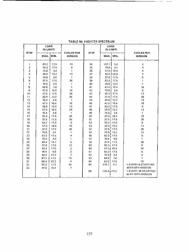
TABLE 9d FIGHTER SPECTRUM

LOAD LOAD

(% LIMIT) (% LIMIT)

STEP CYCLES PER STEP ---- CYCLESSPERMAX. MIN. MISSION MAXMIN. MISSION

I I1 63.2 I 17.5 10 34 103.1 j 5.8 1

2 55.3 17.5 9 35 70.8 3.4 53 70.8 3.4 1 36 47.0 16.4 4

4 28.9 13.2 13 37 46.5 1-18.9 1

5 70.8 3.4 1 38 37.51 17.5 5

6 37.5 17.5 39 39 63.2 175 1

7 70.8 3.4 1 40 28.9 13.2 1

8 84.8 7.0 1 41 47.0 16.4 169 47.0 I 16.4 18 42 70.8 3.4 3

10 37.5 17.5 39 43 55.31 17.5 13

11 28.9 I 13.2 26 44 37.51 17.5 3912 76.4 I 4.6 1 45 28.91 13.2 13

13 47.0 I 16.4 18 46 47.01 16.4 18

14 28.9 I 13.2 13 47 63.2 17.5 515 47.0 16.4 19 48 28.91 13.2 13

16 76.4 4.6 1 49 70.8 3.4 117 55.3 17.5 28 50 47.0 16.4 19

18 37.5 17.5 39 51 37.51 17.5 39

19 63.2 I 17.5 5 52 55.3 17.5 9

20 47.0 I 16.4 19 53 28.9 13.2 13

21 37.5 I 17.5 39 54 37.51 17.5 3922 70.8 3.4 1 55 28.91 132 13

23 63.2 17.5 4 56 63.2 17.5 5

24 76.4 4.6 1 57 76.4' 4.6 125 94.4 14.7 5 58 37.5 17.5 39

26 37.5 17.5 12 59 55.3 17.5 9

27 63.2 17.5 2 60 47.01 16.4 36

28 76.4 4.6 2 61 55.31 17.5 929 66.4 22.2 7 62 70.8 I 3.4 3

30 63.2 I 17.5 10 63 84.81 7.0 131 66.4 I 22.2 4 64 63.21 17.5 10

32 55.3 I 17.5 30 65 118.1 4.1 1 EVERY 6 STARTING33 47.0 16.4 7 WITH 6TH MISSIONI 66 120.4 1-14.2 1 EVERY 18 STARTING

I WITH 18TH MISSION

258

TABLE 10 UNDERLOAD AND COMPRESSION SPIKE TEST PLAN

SPECIMEN NO. COMPR/ TENS/ COMPR/ OVER/ UNDER/ONLY COMPR TENS UNDER OVER

AD-25-115 XAD-25-116 XAD-25-117 X(1)

TD-25-117 X(1)TD-25-118 XTD-25-119 X

AG-25- 8P XAG-25- 9P X XAG-25-10P X X

TG-25- IP XTG-25- 4P X X

(1) Multiple Overloads before Underload

TABLE 11 MEASURED AND CALCULATED STABLETEAR, SPECIMEN AG-25-6P

SURFACE CRACK KmaxoL MEASURED FROMLENGTH AFTER (ON FRACTURE RESISTANCEOVERLOAD (IN.) ( KS IVI/i SURFACE) CURVE

.633 30.4 .003 .00

.852 36.3 .007 .0081.045 41.4 .020 .0231.282 47.9 .044 .0521.532 55.5 .095 .105

TABLE 12 MECHANICAL PROPERTY RESULTS

MATERIAL 2219-T851 Ti 6A1 - 4V TITANIUMALUMINUM

THICKNESS (INCH) 1/4 1/4 3/4

TENSILE ULTIMATE (KSI) 66.9 132.6 137.6TENSILE YIELD (KSI) 54.7 130.0 135.3*ELONGATION AT FAILURE (%) 10.3 17.8 12.6NUMBER OF TESTS 6 4 4

Gage length = 2 inches

259

TABLE 13 COMPARISON OF CRACK GROWTH RATES

AS A FUNCTION OF R FOR 2219-T851 ALUMINUM

STRESS CRACK GROWTH RATE, da/dN (IN./CYCLE) @ K = 15 KSI IN"

RATIO EQ 19a EQ la EQ lb EQ 2

R EQ 21

-1 2.18 x 10-6 2.18 x 10-6

0 1.66x 10.5 1.66x 10-

5

.2 2.52 x 10"5 2.43 x 10-5

.4 3.57 x 10,5 3.41 x 10.5

.5 4.00x 10-5 4.0 x 10-5

.6 4.08 x 10-5 4.0 x 10-5

.7 3.38 x 10-5 4.0 x 10-5

KMAX = 15 ksi %/- FOR ALL VALUES OF R-..-I

1--R

TABLE 14 COMPARISON OF CRACK GROWTH RATES ASA FUNCTION OF R FOR Ti 6A1-4V TITANIUM

STRESS CRACK GROWTH RATE, da/dN (IN./CYCLE) @ K =15 KSI INW

RATIO EQ 19a EQ 1c EQ3

R EQ 21

-1 3.44 x 10-6 4.65 x 10-6

0 2.47 x 10-6 2.47 x 10-6

.3 4.37 x 10-6 4.45 x 10-6

.5 6.26 x 10-6 6.23 x 10-6

.7 8.62 x 10-6 8.45 x 10 6

15 ksifImax 1-R for all values of R --- -1

260

TABLE 15 COMPARISON OF TEST AND PREDICTED LIVES FORSINGLE PERIODIC OVERLOAD TESTS

MATERIAL SPECIMEN OVERLOAD CYCLES OF CYCLES REQUIRED TO PREDICTED LIFENO. RATIO, O/L LOW LOAD REACH a = 1.6 IN TEST LIFE

BETWEEN TEST PREDICTION (AT a = 1.6 INCHES)OVERLOADS

AD-25-26 1.8 500 238,000 (2)-38 1.8 500 390,000 1,500,000 3.98

2219-T851 -43 1.8 1000 142,000(1) 430,400 3.04ALUMINUM -29 1.25 50 160,000 (2)

-45 1.25 50 126,000 290,000 2.30-27 1.25 100 75,500 75,500 1.00

TD-25-30 1.8 500 323,000 212,000 .66-37 1.8 500 445,000 235,000 .53

Ti 6A1-4V -28 1.8 1000 -900,000 195,000 .22TITANIUM -32 1.25 50 210,000 265,000 1.26

-39 1.25 50 214,000 248,000 1.16-31 1.25 100 207,000 241,000 1.16

(1) afinal = 1.3 in.

(2) Prediction terminated

Table 16 - Values of C' and n' used in Equation 39 for Predictionsin Figure 223 when a= 2.6 andf8= 0.10

REF. FIGURE 223 FOR EQUATION (39)CASE x y C' n,

1 0 50 2.571 x 10- 2.1192 50 0 1.223x10-2 2.1023 1 50 1.138x 10-3 2.2634 3 50 1.563 x 10-3 2.0665 6 50 2.249 x 10-3 2.0636 10 50 3.289 x 10-3 2.0887 25 50 6.962 x 10-3 2.0968 50 50 1.321 x 10-2 2.105

261

APPENDIX A - EQUATIONS

The equations which are referred to most frequently in the text arepresented here for reference.

da =9 .6R)AKj 0 _< R _• 0.5 (la)S-= 1.96 x 10 [(i+d-N

3.3I4

= 1.96 x 10-9 [1.3AK] R > 0.5 (ib)

-10 3.085.9 x 10 [(l + .7R)AK] 0 < R < 0.7 (ic)

3.34

2.6 x 10- 9 [Kmax] R = -1 (2)

3.08 R=- 3

= 1.11 x 10-9 [Kmax] R = -1 (3)

K -Kmax2 max1

f 0/L • K - Kmax2 maxI

where:

P Pmin 1 in 2

P O/L • Pmax 1 max2

ASeff = Smax - Sc = Smax (i - Cf) (15)

SCf - sc (16)

max

262

d a max- [S v# (19)

Cf= cf-i+ (c f f (i +R)P (21)

where for:

2219-T851 Ti 6AI-4vAluminum Titanium

cf .4o .4o

C .347 .332

p 3.93 3.33

B

S 1 (= -Se)( ) (22) S

Y +(i- y +s-Nt-1 (26)

where for:

2219-T851 Ti 6A1-4vAluminum Titanium

.67 .80

N sat 13 100

AKeff = (S - Sr) • (30)

263

S r •S (32)r

n

S S a F (asin ' - sin- (I -a - p y a

dN F 21(7a_ T (a a )(- a - p

I T_ f_ sin-I + 1_2

264

APPENDIX B - COMPUTER PROGRAM

The Crack Closure Model developed during this program, called sub-routine CLOSUR, was mated to the CRACKS 2 computer program. The combinedprograms have been checked out on both IBM and CDC facilities although only

the CDC program is available for general usage. The CRACKS 2 CDC computerprogram was converted to run on the IBM system 360/70 computer. In order to -

perform this conversion, the following changes were required:

9 All A10 formats became 2A4, A2. Whenever this was required, thenecessary redimensioning was included. A result of this operationwas that DATA statements defining those variables were replacedwith REAL type statements which included the appropriate dimen-

sioning. In addition, where the original program tested againsta single variable, now a three-part logical IF statement isrequired.

* All variable and program names exceeding six characters werecontracted to six characters. The equivalences between the original

and contracted names are tabulated as comments at the beginning ofeach program.

These changes were retained when the composite program was re-converted toCDC.

B-1 MODIFICATIONS TO CRACKS 2

The addition of the Crack Closure Model was achieved in as straight-forward a manner as possible and can be considered to be a comparativelyindependent subroutine. It does interface with the CRACKS 2 program at appro-priate locations. These include the following subroutine programs:

Name Type

MAIN

INPUT SubroutineOUTPUT SubroutineGRWCRK (GROWCRK) SubroutineBETAS SubroutineRY Real function

NOTE: Names in ( ) shortened to six characters for IBM 360.

A flow chart showing the overall path through the program is presentedin Figure B-1. Links between original CRACKS 2 subroutines or subroutinescalled by CLOSUR are not shown.

265

Changes to the original program in order to implement CLOSURE wereminimal. These are described below.

MAIN - No changes.

INPUT - Added:

1. Common blocks CLOS and CLOSIC. Also REAL NSAT.

2. Initial conditions immediately following common information.

3. The CLOSUR option was defined as model three. Subsequent to

statement 523, READ/WRITE statements introduced to read additionalinput required and print out appropriate information. The READstatement uses existing format 1020. Format statements 2107 and2108 were added for output.

4. Appropriate READ/WRITE statements following statements 537 and538 to read BETA factors 7 and 8. These are described under BETAS.Formats 2206 and 2207 were added for new BETA functions.

5. The Crack Closure Model accepts negative loads.- Therefore, appro-priate statements were introduced between statements 600 and 650to circumvent instructions setting negative stresses equal to zerowhenever MODEL = 3.

OUTPUT - No changes.

GRWCRK - Immediately following statement 130, added: CALL CLOSUR (CYC, A,DN)

BETAS - These two new stress intensity solutions for compact tension specimenswere added. Type 7 is the ASTM standard geometry compact specimen.The stress intensity expression was taken from Equation 12 of Refer-ence B-l. Type 8 is for the Grumman compact tension specimen geometryused in this program. The stress intensity solution is described inAppendix C.

RY - No changes.

B-2 ADDITIONAL INPUT DATA REQUIREMENTS

No changes were made to the basic input data format. Additions wererequired. The following descriptions refer to the tables of Reference B-2.Table 3 - If CONl (Model) on RETARD card is 3., one additional input card isrequired. This card immediately follows the RETARD card. All other variableson the RETARD card remain the same. The new card contains the following var-iables and a description of their relationship to equations within thisreport, Section 4. The format is number 1020 in INPUT, 8El0.0.

266

The card contains: CF, CCOEF, CFEXP, B, BOL, NSAT

Program EquivalentName Name Description

CF Cf Equation 210

CCOEF Cf Equation 21

CFEXP p Equation 21

B B Equation 22

BOL YI Equation 26

NSAT Nsat Equation 26

Description of BETA following Table 3 - There, type 7 and 8 BETAfunctions were added. The type 7 factor is for the ASTM standard geometrywhile the type 8 factor is for the Grumman compact tension geometry used inthe test program. The format remains the same as for type 1 for example, withthe following definitions:

CON 1 - Specimen type (7. or 8.)

CON 2 - Specimen width - reference Figure 2 of this report

CON 3 - Specimen thickness

CON h- a.)S4- Same as existing definitions

CON 5 - af I

Whenever these BETA factors are employed, the input stresses are replaced byloads. That is, simply assume the equivalence S = P. The loads are eitherin pounds or kips to be compatible with the crack growth equation parametersselected.

B-3 DESCRIPTION OF SUBROUTINE CLOSUR

The CLOSUR subroutine contains its own integration and crack growthrate calculation routines.

The integration routine is implemented only if the closure level isdecreasing (retarded growth) or constant (constant amplitude growth) and thenumber of cycles in the current layer is greater than or equal to 20. The

267

routine only applies to the current layer and does not integrate overallflight growth. It assumes that, for small increments of crack extension (arbi-trarily selected as 10% of the current crack length), the crack growth ratefollows the law:

da C an (B-1)

dN

within a given load layer. The parameters C and n are evaluated by calculat-ing the crack growth rates at crack lengths a. and af. There, a. is the

1I 1

current crack length and af is either 1.1 a. or a , whichever is less. As

described in Section 4 of this report, a is the location of the elastic-

plastic interface. Then, given C and n, Equation B-1 is integrated to obtainAN:

AN - C (1--n) L n - a.l - n] (B-2)

11The value of AN is the number of cycles required for the crack to propagatefrom a.1 to a f. If AN is less than N, the number of cycles in the current

layer, a., is set equal to a and the process is repeated. When the accumu-I f

lation of ANs exceeds N, Equation B-2 is evaluated for af in the last defini-

tion so that Z AN = N. Control is then returned to GRWCRK.

The Crack Closure Model intrinsically contains a stress ratio effecton crack growth rates. As a result, only the bi-linear Paris and tabular da/dNvs. AK input formats are accepted and used by CLOSUR. If either the Walker orForman equations are called with CLOSUR, a diagnostic message is printed andexecution of the problem is terminated. As a convenience, the subroutine RATE

is not called by CLOSUR and the crack growth rates are calculated withinCLOSUR, CLOSUR calls BETAS and RY as required.

An overall flow chart for CLOSUR is presented in Figure B-2 while thecomputer listing is presented in Table B-1,

REFERENCES

B-1 Newman, Jr., J. C., "Stress Analysis of the Compact Specimen Includingthe Effects of Pin Loading", Presented at the ASTM Seventh NationalSymposium on Fracture Mechanics, College Park, Maryland, August 1973.

B-2 Engle, R. M., "CRACKS II Input Instructions", 13 November 1973.

268

L '[,NPUT•,N I ;OUTPUTI

GRWCRK

B ETASCLOSUR

RY

Fig. B-1 Overall Flow Chart of Modified CRACKS 2 Program

SFUNCTIONS i

CONDITIONS •L.B

100 CALCULATE P MINIMUM STRESS ADJUSTMENTINITIAL ANDFINAL CLOSUREBEALEVELS - TEST FOR AKeff > DELKTH

5013 DETERMINE IF 6000 I

INTEGRATION IS SINTEGRATIO

205 APPLICABLE 6280' ROUTINE•NO 45 E A

205 CYCLE-BY-CYCLE O WTHRATE ROUTINE'CRACK GROWTHTETFR

310 ANALYSIS A > AMAXS~~KM-AX >__ KQI• ~PROPER

LGROWTH EQUATION,

NOTE:

311 UPDATE: CLOSURE 4--B NUMBERS NEAR BOXES AREST R ESS, AP, STATEMENT NUMBERS AT

50 INITIAL CONDITIONS RY APPROXIMATE BEGINNINGAND END OF EACH ROUTINE.

Fig. B-2 Subroutine CLOSUR Flow Chart

269

TABLE B-i CLOSUR SUBROUTINE, SHEET 1 OF 8

SUPROUTINE CLOSUR(CYC9AI9DN)CCCC INCLUDES MODIFICATION 4 OF SMALLC SEPT 49 1974CCC EQUIVALENCE BETWEEN CRACKS 2 AND CLOSURC CRACKS 2 CLOSURC ASUBP APC SMAX SC CYCLES CYCLSC ISEGIC J4KC SMALLN AN (NOT USED AS SMALLN ANYWAY)C KSURO AKCC DELKTH KTHc A AlC AMAX AFCC

COMMON/DATA/ EQNNASAJlPRTJ2PRTJ3PRT ,J4PRTAZEROAF.NZEROINTEGER EONREAL NZEROCOMMON/RDATA/ MODEL ,RETARDPLSTRNCVLDSIGMAXSIGMIN ,APSMALLMINTEGER RETARDPLSTRNCOMIMON/MDATA/ M'ATID(20),C,)ANCARRAY(lO0),SNARAY(lO0),KSURC,

/AKCSIGMAY, KTHsRMULT9RCUTsOLMAXREAL KSURCCO;MMON/LDATA/ S(100,50),SMIN(100,950),CYCLS(10OO,50),NLYRS(50)s

/ ~NFRLKSIRLKS( 1000) ISEGS(1OC0) ,NSEGSCOMMON/STEDS/ KJlJ2,J3,IISTOPIRSTRTNORTRDCOMMON/CORFAC/ ISURFRATIO,%PHITHICKIBETA(1O)oBETA(1O),NPTS,

/ AOVERB(100),BTABLE(100),NPTS2,AOVRB2(100),/ RýTABL2(l0O),ASTART(1O),ASTOP(10)

COMMON/PAR IS/ClSNlDKCOvC2,5N2COMMVON /DIREICT/ NCADNCOMNI',ON/OU)TPOT/XK,XKA ,XKEFFNREAL KYAX ,KYAXACOý-IMON/CLOS/CFCCOEFCFEXPBBOLNSATCOM'-.1ON,\/CLOSIC/SCSPEAKPRVMXAPEAKSC1,SC2,SC3,PRVMN.r)ATA PI/3ol4l59265/REAL ISUM,"KTHSGKCOEFKEXPNOL ,NSATNPRNPREVKTHDIMENSION )(6)9Q0O(2)

CCCC CLOSURE FUNCTION

CLOSE(GlG2) = Gl*(CCOEF + (CF - CCOEF)*(lo + G2)**CFEXP)CC FUNCTION FOR SC LT OR EQ SC INITIAL

DOWN(Z1,Z2oZ3) = Zl - (Z1-SC3)*(Z2/Z3)**B

270

TABLE B-i CLOSUR SUBROUTINE, SHEET 2 OF 8

CC FUNCTIONS FOR SC GT SC INITIAL

SCONF(SC3) = SC3*ROLCC FUNCTION FOR INCREASING CLOSURE STRESS

NPREV(SCqSC39SCll) =l.+(NSAT-1. )*(SC-SCll)/(SC3-SCll)CCCC INITIALIZE PARAMETERS

IGIROW = 0MODE =0ITEM = 11 G R-O W = 1

CYSUM = CYCLS(ItK)NOL = 0.ASTRT =AlKLU =1R =0.

IF (S(IK) *NE, 0.s R SMIN(I#K)/SCIsK)SMNGP. = SMIN(IsK)

IF C SPEAK *NE. 0. GO TO 30SINITL =S(I*K)IF CSINITL *LE* 0s) SINITL 0*05*SIGMAYR =SMIN(IsK)/SINITL

CALL 8ETASCS(IqK)9AlqALP9QE)XK = SINITL*SQRT(PI*Al)*ALPGl = SINITLG2 = R

IF (G2 *LT* -1s) G2 =-16SC =CLOSECGlsG2)sci = SCSC2 = S CSC3 =SCSPEAK = SINITLPRVMX = SINITLPRVMN = SMIN(IsK)APEAK =AlAP =Al + RYCXKPLSTRN)OMGA2 = AP

30 CONTINUECCC START ANALYSIS

100r ISUM =0.CC

61 = S(IK)G2 = R

IF ( 62 + 1.e 104,105,105104 62 =-1.

105 SC3 =CLOSE(G~lsG2)IF(SMIN(I9K) - PRVMN) 5003960960

C MINIMUM STRESS ADJUSTMENT5003 CONTINUE

PRVMN = SMIN(ItK)

271

TABLE B-I CLOSUR SUBROUTINE, SHEET 3 OF 8

GI 6 SPEAKG2 = SMIN(I9K)/SPEAK

IF (G2 + 1.) 5005,5006,50065005 G2 = -le5006 SCI = CLOSE(G1,G2)

G1 = PRVMXG2 = SMIN(ItK)/PRVMX

IF (G2 + l.) 57,58,5857 G2 = -1o58 SC3 CLOSE(G1,G2)

G3 = ASTRT - APEAKG4 = AP - APEAKSC2T = DOWN(SClG3tG4)

IF(SC2T - SC2) 59,6096059 SC2 SC2T60 SC = SC2

IF(S(I*K)-SC2) 450,450,50095009 SMNGR = SC2

IF (SMIN(ItK)-SC2) 501095011950115010 SMNGR = 5C25011 CALL BETAS(S(IK)9AltALP#QE)

XKEFF=(S(IK)-SMNGR)*SQRT(PI*A1)*ALPIF((XKEFF/(1.-RMULT*R)/(1.-CF))-KTH) 450,450,5012

5012 G6 = S(ItK)G2 = R

IF (G2 + 1.) 93,9499493 G2 : -1.94 SC3 CLOSE(GloG2)

IF ( S(IK) - SC3 ) 9599699695 SC3 = S(IK)96 CONTINUE

IF(S(IK) - SPEAK) 9095013,50135013 KLU = 3

CC INITIALIZATION FOR INTEGRATION ROUTINECC MODE = 1 IF CYCLS(IK) eLT. 20 AND SC3 oLE. SCC MODE = 2 IF CYCLS(IK) *LT* 20 AND SC3 oGT. SCC MODE = 3 IF CYCLS(IK) *GE* 20, SC3.GT.SC AND NoLT.NSATC MODE = 4 IF CYCLS(IK) *GE, 20 AND SC3 *LT. SCC MODE = 5 IF CYCLS(IK) *GE. 20 AND SC3 = SCC INTEGRATION PERFORMED FOR MODE = 4 AND 5

90 MODE = 5IF ( CYCLS(IK) - 20. ) 201,203,203

201 MODE = 1IF ( SC - SC3 ) 202,205,205

202 MODE = 2GO TO 205

203 IF C SC *EQo SC3 ) GO TO 205MODE = 3

IF ( SC3 - SC ) 204,205,205204 MODE = 4205 CONTINUE

CC

DCYC = CYCLS(IK)/30000.

272

TABLE B-1 CLOSUR SUBROUTINE, SHEET 4 OF 8

IF ( DCYC ,LTo 1.0 ) DCYC = 1.0NNCYC = CYCLS(IK)/DCYC

CC START CYCLE - BY - CYCLE ANALYSISC

DO 310 J = 19NNCYCIF ( MODE - 3 ) 2109210,6000

210 IF (SC3 - SC) 92092*11192 GO TO (1O191609101,O1)tKLU

101 IF (OMGA1) 501495015s50155014 OMGA1 = O05015 IF (OMGA1/OMGA2 - 1.) 5017o5017,50165016 OMGAI = OMGA25017 SC = DOWNCSC2oOMGAlOMGA2)

111 IF(SMIN(I9K} - SCO 5023,160,1605023 SMNGR = SC160 CONTINUE

GO TO 40504051 CONTINUE

ISUM = ISUM + DCYCCYC = CYC + DCYCCYSUM = CYSUM - DCYCDN = CYSUM

GO TO (138,501,50It50I)9ITEM138 CONTINUE

IF ( MODE - 2 ) 143,1449144143 OMGAI = Al - ASTRT

IF (Al - AP) 300,141,141141 KLU = 2

SC = SC3AP = Al

GO TO 300144 SC1l SCONE(SC3)

NPR = NPREV(SCoSC39SC11)IF ( NPR ) 145,146,146

145 NPR = 0.146 NOL = NPR + DCYC

SC = SCI1 + (SC3-SC11)*(NOL-1.)/(NSAT-1.)IF ( SC3 - SC 147o147,300

147 SC = SC3IF ( MODE - 2 ) 3009300,148

148 MODE = 5300 CONTINUE310 CONTINUE311 CONTINUE

PRVMX = S(IK)SC2 = SC

GO TO C501,4009400#400)9KLU,400 CALL BETAS(S(I9K)qAI9ALP9QE)

XK = S(IK)*SQRT{PI*A1)*ALPAP = Al + RY(XKtPLSTRN)APEAK = AlSPEAK = S(IK)PRVMN = SMIN(I#K)

IF (SC3 - SC) 420o420,430420 SC1 = SC3

GO TO 501

273

TABLE B-i CLOSUR SUBROUTINE, SHEET 5 OF 8

430 SCi = SCGO TO 501

450 ISUM =ISUM + CYCLS(IsK)

CYC CYC +CYCLS(I#K)DN = 0

501 CONTINUEC

GO T0C500#60096209503)sITEM503 ISTOP = 2

Al = ATRANS/(2**RATIO)WRITE(6,l) AICYC

1 FORMAT(1HO,120(lH*)/25X,55HTRANSITIONTFO A THRU CRACK OF EFFECTIVE1 LFNGTH# AEFF 9F9s594H AT 9F12*297H CYCLES /#lXtl20(lH*))

GO TO 50CCC END OF CYCLE BY CYCLE ROUTINEC

500 CONTINUEGO TO 50

C Al EXCEEDED AF (AMAX)600 ISTOP =1

GO TO 50620 ISTOP =1

WRITE (6.7)7 FORMlAT(IHO,12OC1H*)/25XA6HKMAX APPLIED EXCEEDS KSUBO. PROBLEM TER1MINATED/1X,120(1H*)/lHO,24X,26HLAST CALCULATED VALUES ARE///)

DELTAK = XK*(1.-R)WRITEC698) J1tJ2,I .J3,KCYCAlXKXKEFF.DELTAKDADN

8 FORMAT(25X918HBLOCK IN SPECTRUM 914// 25X918HFLIGHT NUMB3ER P14//25X918HMISSION NUMBER t14//25X9lSHPASS OF MISSION o14//25X918HLAYER IN MISSION 914/

5 25X .18HACCUMULATED CYCLES.E16o8/6 25X#18HCRACK LENGTH oEl6o8/7 25X,18HKMAX APPLIED PE16*8/8 25X#18HKMAX EFFECTIVE *E16*8/9 25X,18HDELTA K *E16*8/

/25XolBHDA/DN 9E1698)CC

50 CONTINUEXKA = XK

RETURNCCC GROWTH CALCULATIONS4050 CONTINUE

C CHECK FOR XK (KMAXA) *GE* AKC (KSUBQ)CALL AETAS(S(I9K)#AlsALPoOE)

XK =SCIsK) *SQRT(pI*Al)*ALPIF(X"K -AKC) 40629406094060

4060 ITEM = 3DADN = 06

GO TO (502,502*502,406294062)9MODE4062 XKEFF = (S(IsK) - SMNGR)*SQRT(PI*Al)*ALP

274i

TABLE B-1 CLOSUR SUBROUTINE, SHEET 6 OF 8

XKEFFN = XKEFF/(1,-CF)IF ( EQN oEQ. 1 GO TO 9000IF ( EON *EQ* 4 ) GO TO 9010IF ( EQN - 2 ) 8000,800098010

8000 CONTINUEC BI-LINEAR PARIS EQUATION

C = ClAN = SN1

IF ( XKEFFN *GE* DKCOM ) C = C2IF ( XKEFFN .GE* DKCOM ) AN SN2

DADN = C*XKEFFN**ANGO TO 8020

C8010 CONTINUE

C TABULAR RATE VALUESDADN = TBLKUP(CARRAYSNARAYNDADNtO10XKEFFN)DADN = 10**DADN

8020 CONTINUEAl = Al + DADN*.DCYC

IF (Al - AF)4064t4063*40634063 ITEM 2

GO TO 5024064 IF ( ISURF *EQ* 0 GO TO 502

ATRANS = THICK - (((XK/SIGMAY)**2o)/(2o*PI))IF ( Al sLTo ATRANS) GO TO 502

ITEM = 4502 GO TO (4051,6060)oIGROW

CCC END OF CRACK GROWTH CALCULATIONSCCCC INTEGRATION ROUTINE

6000 CONTINUEIF C MODE - 4 ) 6010,6010,6020

6010 0(l) = Al0(2) = APZ2 = Al - ASTRTZ3 = AP - ASTRT00(1) = DOWN(SC2sZ29Z3)Q0(2) = SC3

IF ( ISURF oEQ, 0 ) GO TO 6030IF ( 0(2) *LT* THICK ) GO TO 6030

0(2) = THICKZ2 = THICK - ASTRTQQ(2) = DOWN(SC2,Z29Z3)ISTOP = 2

GO TO 60306020 0(1) = Al

0(2) = ll0"*Al00(1) = SC30Q(2) = SC3

275

TABLE B-1 CLOSUR SUBROUTINE, SHEET 7 OF 8

IF C ISURF EQo. 0 ) GO TO 6030IF ( Q(2) *LT. THICK ) GO TO 6030

Q(2) = THICKISTOP = 2

6030 CONTINUESC = 00(1)

DO 6100 KK = 1#2Al = Q(KK)SMNGR = SMIN(IK)

IF ( SMIN(IK) - QQ(KK) ) 6045,6050o60506045 SMNGR = QQ(KK)6050 IGROW = 2

GO TO 40506060 GO TO (6070o6065.6065,6065)9ITEM6065 GO TO (501t6068),KK6068 ITEM = 1

ISTOP = 06070 KKK = KK + 2

KKKK = KK + 40(KKK) = XKEFFQ(KKKK) DADN

6100 CONTINUE02 = (0(3)-0(4))/(Q(1)-0(2))Ql = Q(3) - 02*0(1)Q4 = (ALOG(Q(5)/0(6)))/(ALOG(Q(3)/0(4)))03 = 0(5)/(0(3)**04)05 = 1. - 04DELTN = (Q(4)**Q5 - Q(3)**Q5)/(02*Q3*Q5)

IF ( DELTN - CYSUM ) 620096150,62506150 CONTINUE6200 Al = Q(2)

IF ( AP - Al ) 6210,6210s62206210 AP = Al

KLU = 2MODE = 5

6220 ISUM = ISUM + DELTNCYC = CYC + DELTNCYSUM = CYSUM - DELTNDN = CYSUM

IF ( CYSUM - ,01 ) 6260,6240,62406240 IF C MODE - 4 ) 6010,6010,60206250 0(4) = (Q(3)**05÷CYSUM*02*03*Q5)**II./05)

)(2) = (0(4) -01)/02DELTN = CYSUMISTOP = 0

GO TO 61506260 SC = SC3

IF ( KLU - 2 ) 627096280962806270 Z2 = Al - ASTRT

Z3 = AP -. ASTRTIF (Z3 *LE. 0. ) Z3 = Z2

SC = DOWN(SC2,Z29Z3)6280 GO TO 311

CcC END OF INTEGRATION ROUTINE

276

TABLE B-I CLOSUR SUBROUTINE, SHEET 8 OF 8

CCC DIAGNOSTICS FOR IVPROPER EQN

9000 WRITE(6,9005)9005 FORMAT(IHO,24X#44HCLOSURE MODEL CAN NOT ACCEPT FORMAN EQUATION /

1 40X920HEXECUTION SUPPRESSEDGO TO 9020

9010 WRITEC6.g015)9015 FORMAT(1HO*24X944HCLOSURE MODEL CAN NOT ACCEPT WALKER EQUATION /

I 40X,20HEXECUTION SUPPRESSED9020 ISTOP = I

XKA = XKRETURN

CC

END

277

APPENDIX C - STRESS INTENSITY FACTOR FOR CTB SPECIMEN

The compact tension specimen used by Grumman (CTB) was longer in theloading direction than its ASTM shaped counterpart, CTA. Referring to Figure2, the values of H/W and d/W were 0.95 and 0.60 respectively. An analyticalsolution for this geometry was interpolated from Table 3 of Reference C-1,using W = 2.5 inches. In addition, two aluminum specimens were equipped withclip gages and the stress intensity factors were determined using the methodof Reference C-2. The results, shown in Figure C-1, were fitted to theequation:

2 3

K .1229 + 16.4o98 ()- 37(-39+ 54.7667 wi) (C-l.a)

afor .2 < - • .5

w

2 3 4

Kt114.054 -830.132 + 2327.177 (i) -2890.811 (:) + 1382.306()P

a (C-1b)

for .5 _a- < .8w

where:

K = stress intensityt = specimen thickness

P = applied load

REFERENCES

C-1 Srawley, J.E. and Gross, B., "Stress Intensity Factors for Bend andCompact Specimens", Engineering Fracture Mechanics, Vol. 4, Compendium,1972.

C-2 Paris, P. C. and Sih, G. C. M., "Stress Analysis of Cracks", ASTM STP 381,1965.

278

20-

BA

EQUATION (Cl)

-A

KtP 10-

I N-

®REFERENCE C-2A EXPERIMENT

)II I I

.2 .4 .6 .8aw

Fig. C-1 Stress Intensity Factor For CTB Specimen

279J U. S. GOVERNMENT PRINTING OFFICE: 1976 - 657-630/377