CPU-Scheduling

Whenever the CPU becomes idle, the operating system must select one of the processes in the ready queue to be executed.

The short term scheduler (or CPU scheduler) selects a process to get the processor (CPU) among the processes which are already in memory. (i.e. from the ready queue).

Processor scheduling algorithms try to answer the following crucial question. Which process in the ready queue will get the processor?

In order to answer this, one should consider the relative importance of several performance criteria.

Performance Criteria

CPU utilization - It is defined as: (processor busy time) / (processor busy time + processor idle time)

Throughput – # of processes that complete their execution per time unit.

Turnaround time – The interval from the time of submission to the time of completion of a process.

Waiting time – amount of time a process has been waiting in the ready queue (waiting for I/O device is not counted)

Response time – amount of time it takes from when a request was submitted until the first response is produced, not output.

Performance Criteria

It is desirable that we,

Maximize CPU utilization Maximize throughput Minimize turnaround time Minimize waiting time Minimize response time

Preemptive – Nonpreemptive Scheduling

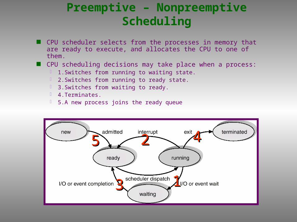
CPU scheduler selects from the processes in memory that are ready to execute, and allocates the CPU to one of them.

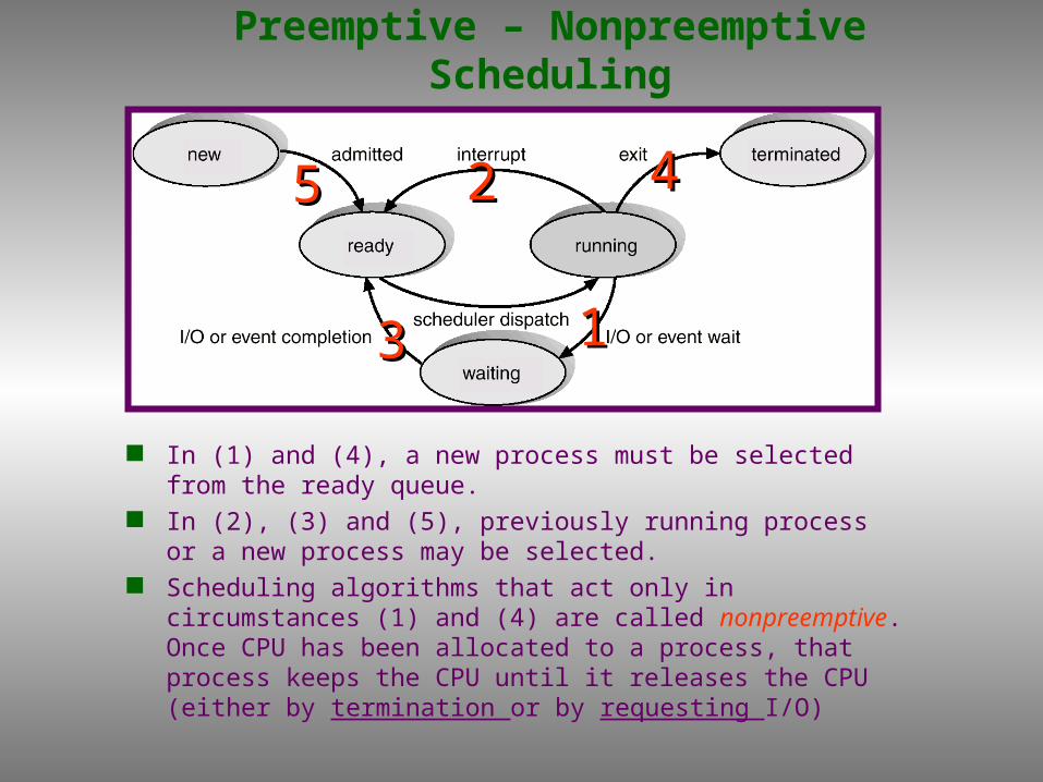
CPU scheduling decisions may take place when a process: 1.Switches from running to waiting state. 2.Switches from running to ready state. 3.Switches from waiting to ready. 4.Terminates. 5.A new process joins the ready queue

11

22

33

4455

Preemptive – Nonpreemptive Scheduling

In (1) and (4), a new process must be selected from the ready queue.

In (2), (3) and (5), previously running process or a new process may be selected.

Scheduling algorithms that act only in circumstances (1) and (4) are called nonpreemptive. Once CPU has been allocated to a process, that process keeps the CPU until it releases the CPU (either by termination or by requesting I/O)

11

22

33

4455

Preemptive – Nonpreemptive Scheduling

A scheduling algorithm which acts on all circumstances is called preemptive. (i.e. such an algorithm can select a new process in circumstances 2, 3 and 5).

The CPU is allocated to the highest-priority process among all ready processes. The scheduler is called each time a process enters the ready state.

Advantages of non-preemptive scheduling algorithms: They cannot lead the system to a race condition. They are simple.

Disadvantage of non-preemptive scheduling algorithms: They do not allow real multiprogramming.

Advantage of preemptive scheduling algorithms: They allow real multiprogramming.

Disadvantages of preemptive scheduling algorithms: They can lead the system to a race condition.

First-Come, First-Served (FCFS) Scheduling

This is the simplest one. In this algorithm the set of ready processes is managed as FIFO (first-in-first-out) Queue. The processes are serviced by the CPU until completion in the order of their entering in the FIFO queue.

Once allocated the CPU, each process keeps it until releasing

either due to termination or requesting I/O.

Example: FCFS Scheduling

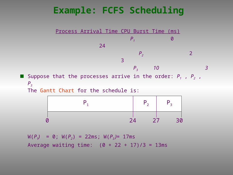
Process Arrival Time CPU Burst Time (ms)

P1 0 24

P2 2 3

P3 10 3

Suppose that the processes arrive in the order: P1 , P2 , P3

The Gantt Chart for the schedule is:

W(P1) = 0; W(P2) = 22ms; W(P3 )= 17ms

Average waiting time: (0 + 22 + 17)/3 = 13ms

P1 P2 P3

24 27 300

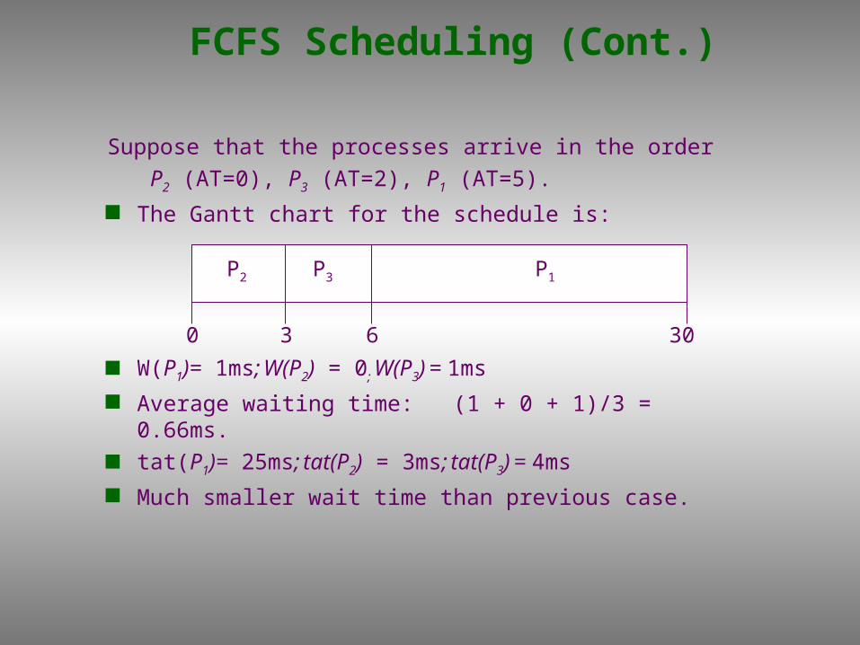
FCFS Scheduling (Cont.)

Suppose that the processes arrive in the order

P2 (AT=0), P3 (AT=2), P1 (AT=5).

The Gantt chart for the schedule is:

W(P1)= 1ms; W(P2) = 0; W(P3) = 1ms

Average waiting time: (1 + 0 + 1)/3 = 0.66ms. tat(P1)= 25ms; tat(P2) = 3ms; tat(P3) = 4ms

Much smaller wait time than previous case.

P1P3P2

63 300

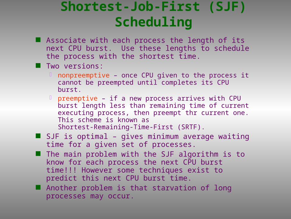
Shortest-Job-First (SJF) Scheduling

Associate with each process the length of its next CPU burst. Use these lengths to schedule the process with the shortest time.

Two versions: nonpreemptive – once CPU given to the process it cannot

be preempted until completes its CPU burst. preemptive – if a new process arrives with CPU burst length

less than remaining time of current executing process, then preempt thr current one. This scheme is known asShortest-Remaining-Time-First (SRTF).

SJF is optimal – gives minimum average waiting time for a given set of processes.

The main problem with the SJF algorithm is to know for each process the next CPU burst time!!! However some techniques exist to predict this next CPU burst time.

Another problem is that starvation of long processes may occur.

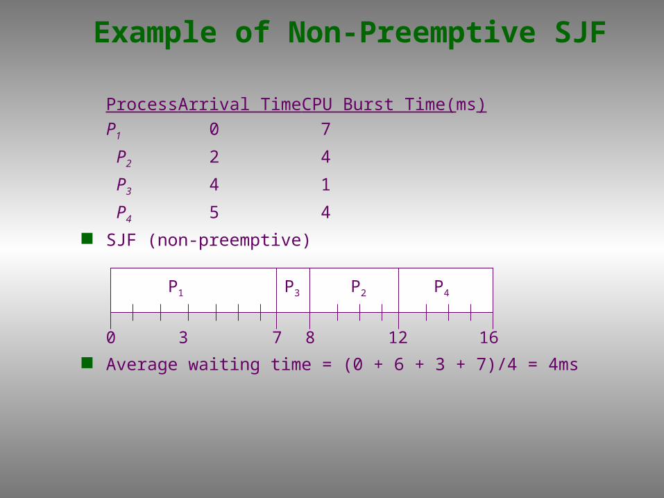
Process Arrival Time CPU Burst Time(ms)

P1 0 7

P2 2 4

P3 4 1

P4 5 4

SJF (non-preemptive)

Average waiting time = (0 + 6 + 3 + 7)/4 = 4ms

Example of Non-Preemptive SJF

P1 P3 P2

73 160

P4

8 12

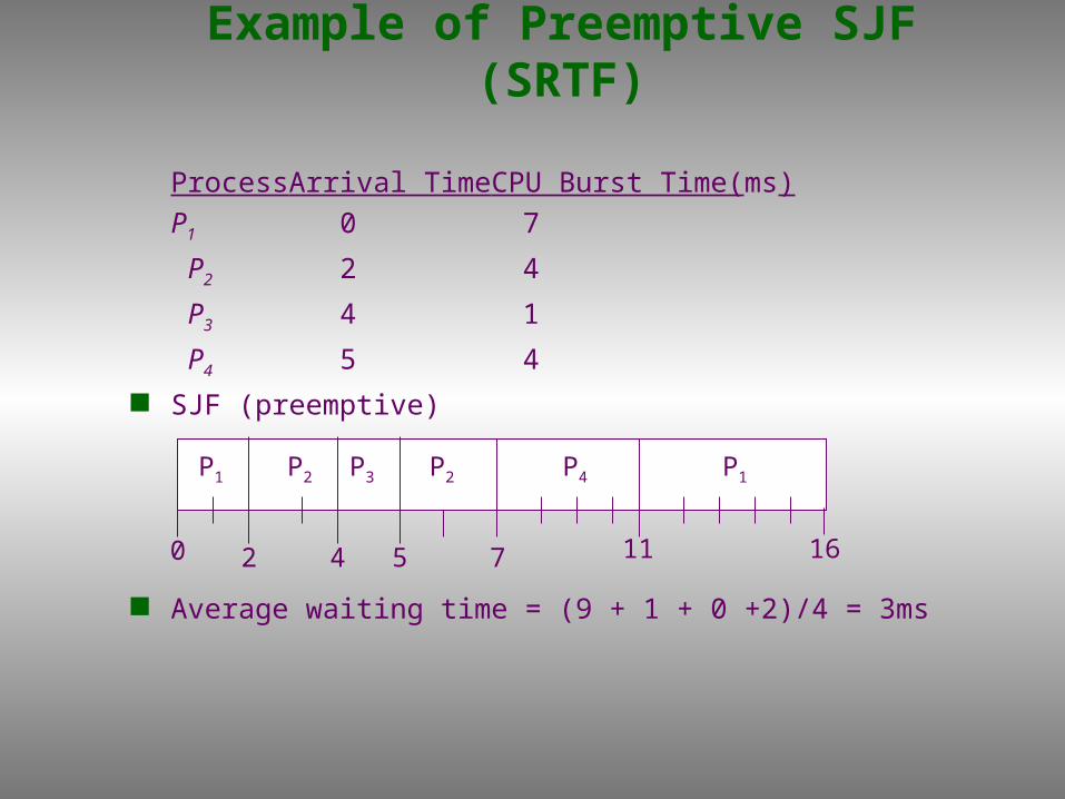
Example of Preemptive SJF (SRTF)

Process Arrival Time CPU Burst Time(ms)

P1 0 7

P2 2 4

P3 4 1

P4 5 4

SJF (preemptive)

Average waiting time = (9 + 1 + 0 +2)/4 = 3ms

P1 P3P2

42 110

P4

5 7

P2 P1

16

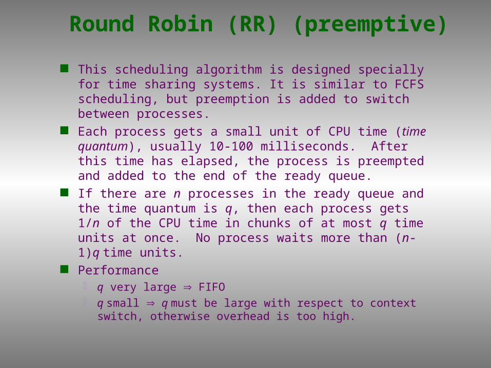
Round Robin (RR) (preemptive)

This scheduling algorithm is designed specially for time sharing systems. It is similar to FCFS scheduling, but preemption is added to switch between processes.

Each process gets a small unit of CPU time (time quantum), usually 10-100 milliseconds. After this time has elapsed, the process is preempted and added to the end of the ready queue.

If there are n processes in the ready queue and the time quantum is q, then each process gets 1/n of the CPU time in chunks of at most q time units at once. No process waits more than (n-1)q time units.

Performance q very large FIFO q small q must be large with respect to context switch,

otherwise overhead is too high.

Round Robin (continue)

The scheduler allocates the CPU to each process in the ready queue for a time interval of up to 1 time quantum in FIFO (circular) fashion. If the process still running at the end of the quantum; it will be preempted from the CPU

A context switch will be executed, and the process will be put at the tail of the ready queue. Then the scheduler will select the next process in the ready queue. However, if the process has blocked or finished before the quantum has elapsed, the scheduler will then proceed with the next process in the ready queue.

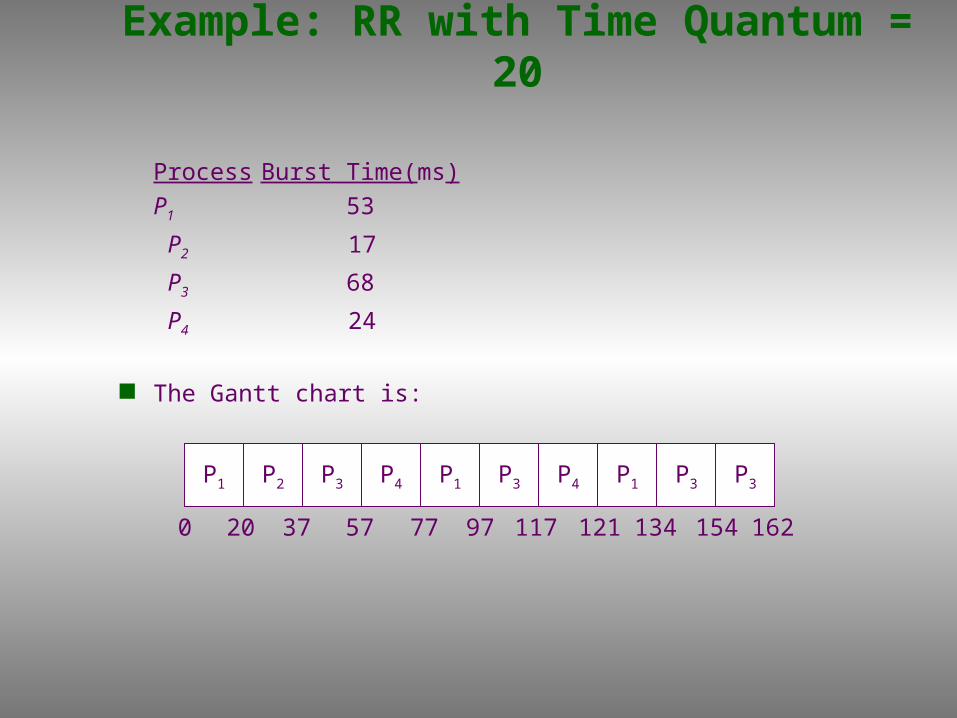
Example: RR with Time Quantum = 20

Process Burst Time(ms)

P1 53

P2 17

P3 68

P4 24

The Gantt chart is:

P1 P2 P3 P4 P1 P3 P4 P1 P3 P3

0 20 37 57 77 97 117 121 134 154 162

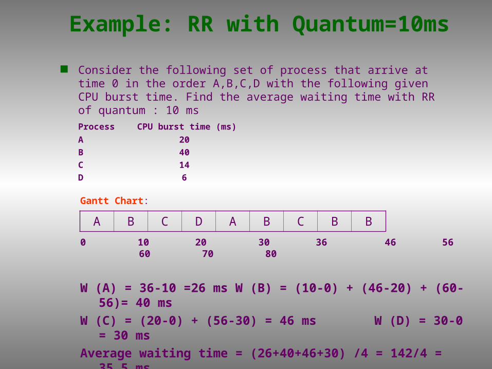
Example: RR with Quantum=10ms

Consider the following set of process that arrive at time 0 in the order A,B,C,D with the following given CPU burst time. Find the average waiting time with RR of quantum : 10 ms

Process CPU burst time (ms)

A 20

B 40

C 14

D 6

A B C D A B C B B

Gantt Chart:

0 10 20 30 36 46 56 60 70 80

W (A) = 36-10 =26 ms W (B) = (10-0) + (46-20) + (60-56)= 40 ms

W (C) = (20-0) + (56-30) = 46 ms W (D) = 30-0 = 30 ms

Average waiting time = (26+40+46+30) /4 = 142/4 = 35.5 ms

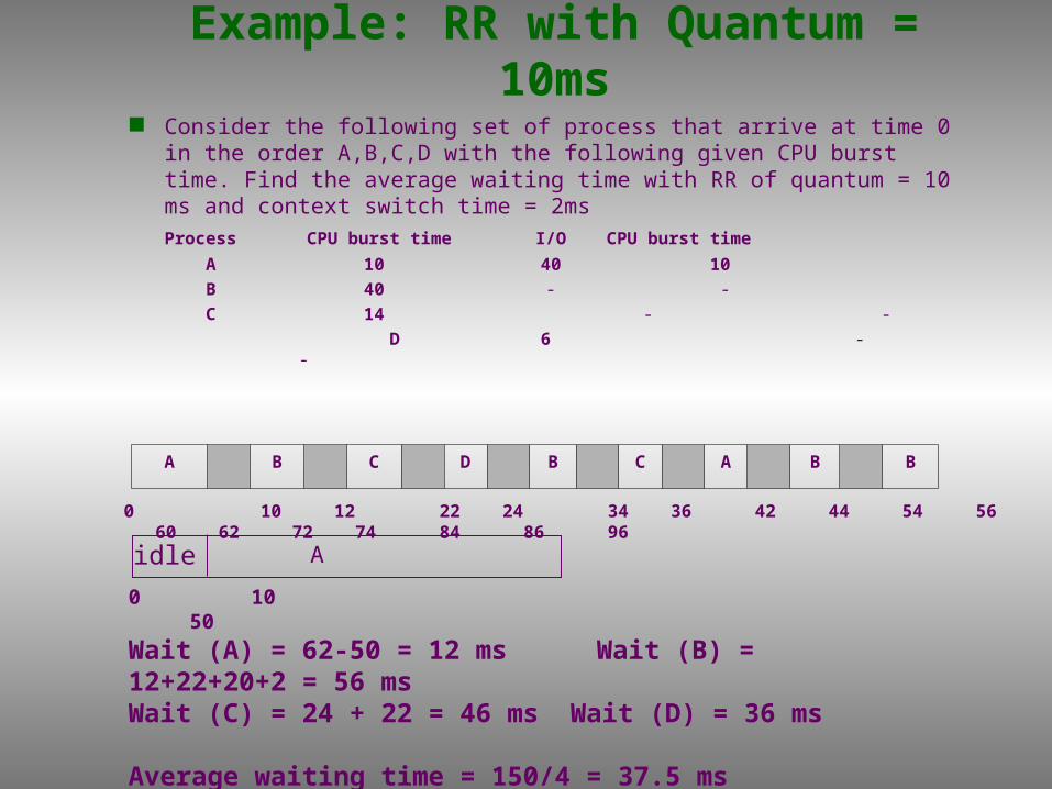
Example: RR with Quantum = 10ms Consider the following set of process that arrive at time 0 in the order

A,B,C,D with the following given CPU burst time. Find the average waiting time with RR of quantum = 10 ms and context switch time = 2msProcess CPU burst time I/O CPU burst time

A 10 40 10

B 40 - -

C 14 - -

D 6 - -

A B C D B C A B B

0 10 12 22 24 34 36 42 44 54 56 60 62 72 74 84 86 96

0 10 50

Wait (A) = 62-50 = 12 ms Wait (B) = 12+22+20+2 = 56 ms Wait (C) = 24 + 22 = 46 ms Wait (D) = 36 ms

Average waiting time = 150/4 = 37.5 ms

Aidle

Priority Scheduling

A priority number (integer) is associated with each process

The CPU is allocated to the process with the highest priority (smallest or largest integer value may be defined as the highest priority). Preemptive nonpreemptive

SJF is a case of the priority scheduling where priority = 1/ (next CPU burst time).

Problem Starvation – low priority processes may never execute.

Solution Aging – as time progresses increase the priority of the process.

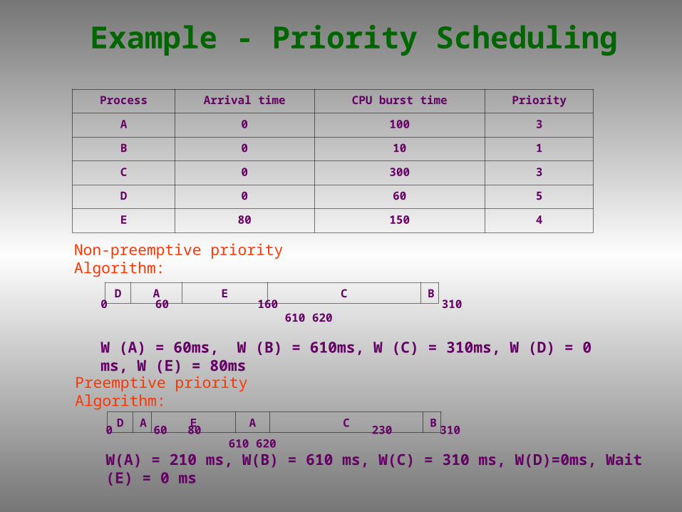
Example - Priority Scheduling

Process Arrival time CPU burst time Priority

A 0 100 3

B 0 10 1

C 0 300 3

D 0 60 5

E 80 150 4

Non-preemptive priority Algorithm:

D A E C B

0 60 160 310 610 620

W (A) = 60ms, W (B) = 610ms, W (C) = 310ms, W (D) = 0 ms, W (E) = 80ms

Preemptive priority Algorithm:

D A E A C B

0 60 80 230 310 610 620

W(A) = 210 ms, W(B) = 610 ms, W(C) = 310 ms, W(D)=0ms, Wait (E) = 0 ms

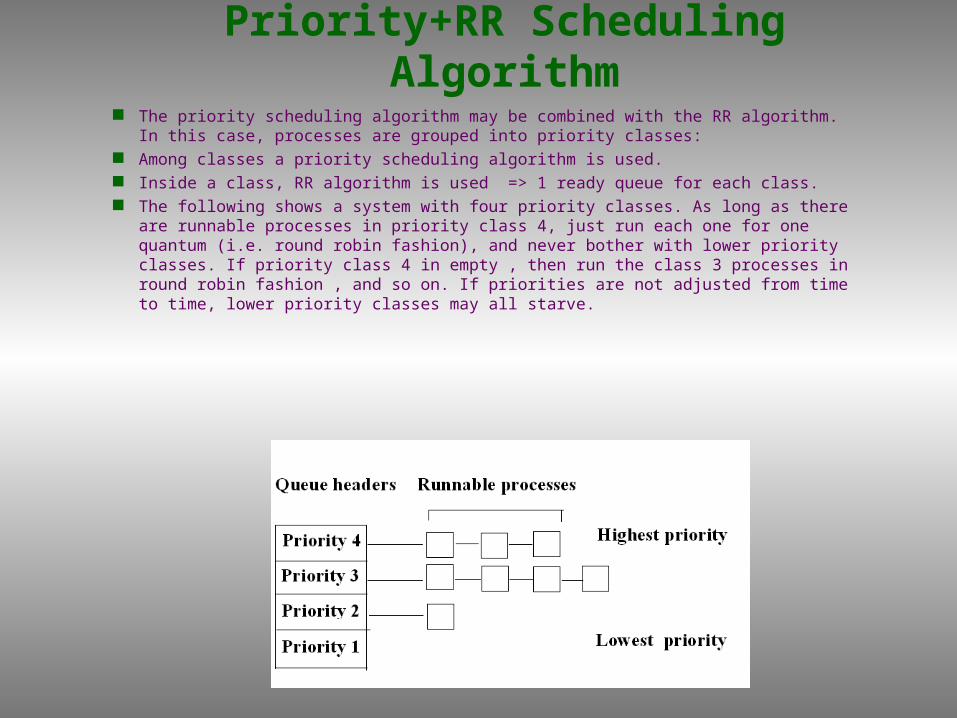
Priority+RR Scheduling Algorithm The priority scheduling algorithm may be combined with the RR algorithm. In this case,

processes are grouped into priority classes: Among classes a priority scheduling algorithm is used. Inside a class, RR algorithm is used => 1 ready queue for each class. The following shows a system with four priority classes. As long as there are runnable

processes in priority class 4, just run each one for one quantum (i.e. round robin fashion), and never bother with lower priority classes. If priority class 4 in empty , then run the class 3 processes in round robin fashion , and so on. If priorities are not adjusted from time to time, lower priority classes may all starve.

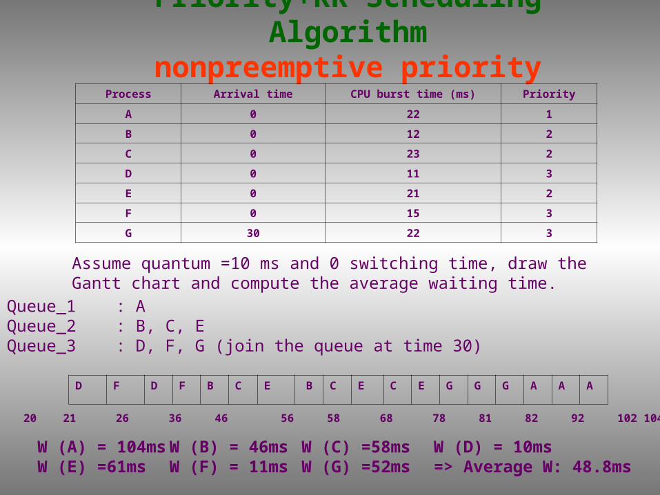
Priority+RR Scheduling Algorithmnonpreemptive priority

Process Arrival time CPU burst time (ms) Priority

A 0 22 1

B 0 12 2

C 0 23 2

D 0 11 3

E 0 21 2

F 0 15 3

G 30 22 3

Assume quantum =10 ms and 0 switching time, draw the Gantt chart and compute the average waiting time.Queue_1 : AQueue_2 : B, C, EQueue_3 : D, F, G (join the queue at time 30)

D F D F B C E B C E C E G G G A A A

0 10 20 21 26 36 46 56 58 68 78 81 82 92 102 104 114 124 126

W (A) = 104ms W (B) = 46ms W (C) =58ms W (D) = 10ms W (E) =61ms W (F) = 11ms W (G) =52ms => Average W: 48.8ms

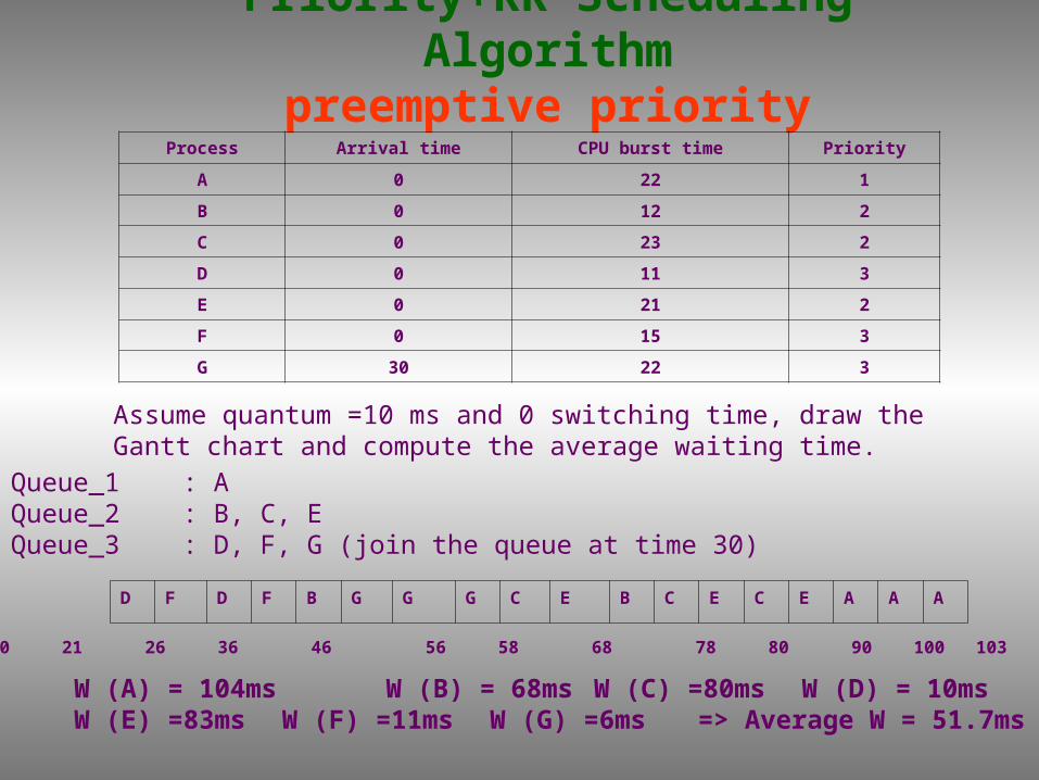
Priority+RR Scheduling Algorithmpreemptive priority

Process Arrival time CPU burst time Priority

A 0 22 1

B 0 12 2

C 0 23 2

D 0 11 3

E 0 21 2

F 0 15 3

G 30 22 3

Assume quantum =10 ms and 0 switching time, draw the Gantt chart and compute the average waiting time.Queue_1 : AQueue_2 : B, C, EQueue_3 : D, F, G (join the queue at time 30)

D F D F B G G G C E B C E C E A A A

0 10 20 21 26 36 46 56 58 68 78 80 90 100 103 104 114 124 126

W (A) = 104ms W (B) = 68ms W (C) =80ms W (D) = 10msW (E) =83ms W (F) =11ms W (G) =6ms => Average W = 51.7ms