cplex optimization studio, modeling, theory, best practices and case studies
TRANSCRIPT

Alkis Vazacopoulos Robert Ashford Optimization Direct
Optimization Direct, CPLEX and Very Large Optimization Models
Summary
• Introduce Optimization Direct Inc. • Explain what we do • Look at getting the most from optimization
• some modeling issues • optimizer issues
• Example of large scale optimization: scheduling heuristic

Optimization Direct
• IBM Business Partner
• Sell CPLEX optimization Studio
• More than 30 years of experience in developing and selling Optimization software
• Experience in implementing optimization technology in all the verticals
• Sold to end users – Fortune 500 companies
• Train our customers to get the maximum out of the IBM software
• Help the customers get a flying start and get the most from optimization and the software right away
Background
• Robert Ashford • Robert co-founded Dash Optimization in 1984. Helped pioneer the
development of new modeling and solution technologies – the first integrated development environment for optimization – in the forefront of technology development driving the size, complexity and scope of applications. Dash was sold in 2008 and Robert continued leading development within Fair Isaac until the Fall of 2010, Dr. Ashford subsequently, co-founded Optimization Direct in 2014.
• Alkis Vazacopoulos • Alkis is a Business Analytics and Optimization expert. From
January 2008 to January 2011 he was Vice President at FICO Research. Prior to that he was the President at Dash Optimization, Inc. where he worked closely with end users, consulting companies, OEMs/ISVs in developing optimization solutions.

Get more from Optimization • Modeling
• Use modeling language and ‘Developer Studio’ environment • Such as OPL and CPLEX Optimization Studio • Easier to build, debug, manage models
• Exploit (data) sparsity • Keep formulations tight
• Optimization • Many models solve out-of-the-box • Others (usually large) models do not
• Tune optimizer • Distributed MIP • Use Heuristics
Modeling: Use Sparsity
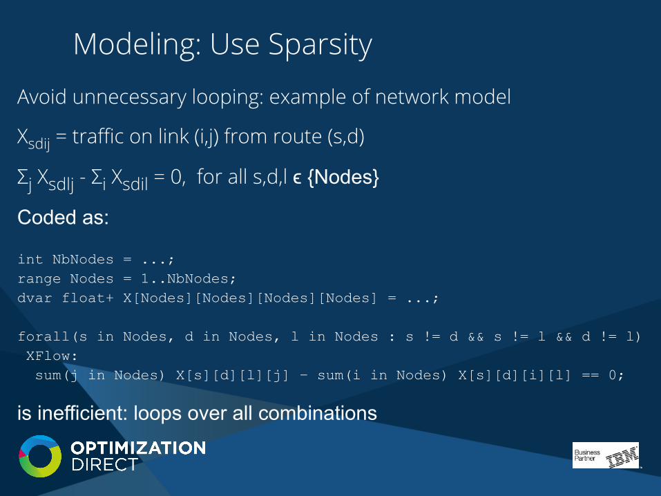
Avoid unnecessary looping: example of network model
Xsdij = traffic on link (i,j) from route (s,d)
Σj Xsdlj - Σi Xsdil = 0, for all s,d,l ϵ {Nodes}
Coded as: int NbNodes = ...; range Nodes = 1..NbNodes; dvar float+ X[Nodes][Nodes][Nodes][Nodes] = ...; forall(s in Nodes, d in Nodes, l in Nodes : s != d && s != l && d != l) XFlow: sum(j in Nodes) X[s][d][l][j] – sum(i in Nodes) X[s][d][i][l] == 0;
is inefficient: loops over all combinations
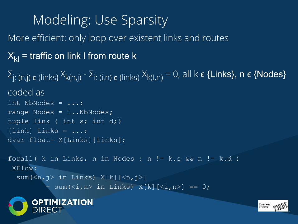
Modeling: Use Sparsity More efficient: only loop over existent links and routes
Xkl = traffic on link l from route k
Σj: (n,j) ϵ {links} Xk(n,j) - Σi: (i,n) ϵ {links} Xk(I,n) = 0, all k ϵ {Links}, n ϵ {Nodes}
coded as int NbNodes = ...; range Nodes = 1..NbNodes; tuple link { int s; int d;} {link} Links = ...; dvar float+ X[Links][Links]; forall( k in Links, n in Nodes : n != k.s && n != k.d ) XFlow: sum(<n,j> in Links) X[k][<n,j>] – sum(<i,n> in Links) X[k][<i,n>] == 0;
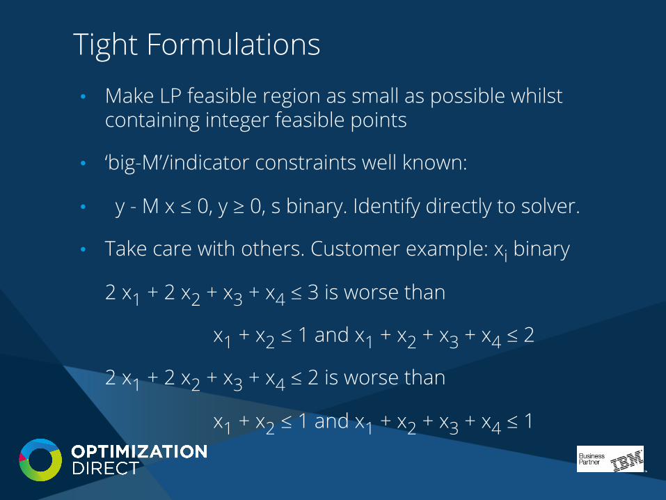
Tight Formulations • Make LP feasible region as small as possible whilst
containing integer feasible points
• ‘big-M’/indicator constraints well known:
• y - M x ≤ 0, y ≥ 0, s binary. Identify directly to solver.
• Take care with others. Customer example: xi binary
2 x1 + 2 x2 + x3 + x4 ≤ 3 is worse than
x1 + x2 ≤ 1 and x1 + x2 + x3 + x4 ≤ 2
2 x1 + 2 x2 + x3 + x4 ≤ 2 is worse than
x1 + x2 ≤ 1 and x1 + x2 + x3 + x4 ≤ 1
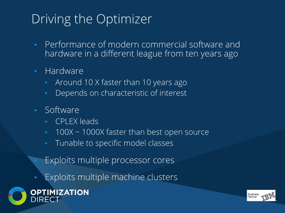
Driving the Optimizer
• Performance of modern commercial software and hardware in a different league from ten years ago
• Hardware • Around 10 X faster than 10 years ago • Depends on characteristic of interest
• Software • CPLEX leads • 100X ~ 1000X faster than best open source • Tunable to specific model classes
• Exploits multiple processor cores
• Exploits multiple machine clusters
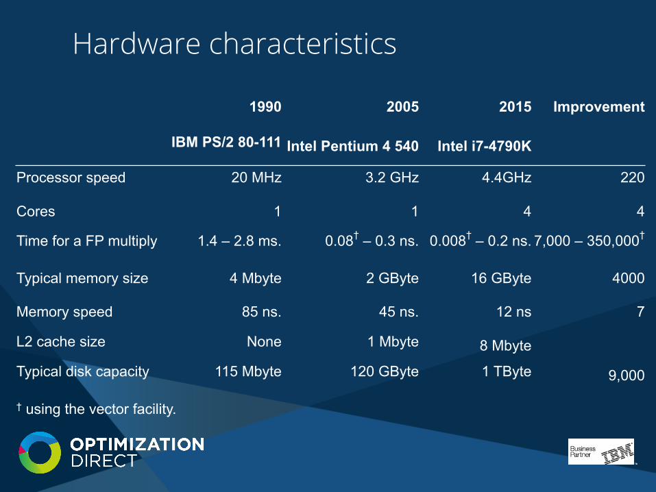
Hardware characteristics
1990 2005 2015 Improvement
IBM PS/2 80-111 Intel Pentium 4 540 Intel i7-4790K
Processor speed 20 MHz 3.2 GHz 4.4GHz 220
Cores 1 1 4 4
Time for a FP multiply 1.4 – 2.8 ms. 0.08† – 0.3 ns. 0.008† – 0.2 ns. 7,000 – 350,000†
Typical memory size 4 Mbyte 2 GByte 16 GByte 4000
Memory speed 85 ns. 45 ns. 12 ns 7
L2 cache size None 1 Mbyte 8 Mbyte
Typical disk capacity 115 Mbyte 120 GByte 1 TByte 9,000
† using the vector facility.
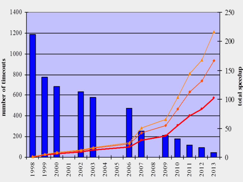
CPLEX Performance Improvements
Where’s the Problem? • Many models now solved routinely which would have
been impossible (‘unsolvable’) a few years ago
• BUT: have super-linear growth of solving effort as model size/complexity increases
• AND: customer models keep getting larger • Globalized business has larger and more complex supply
chain • Optimization expanding into new areas, especially
scheduling • Detailed models easier to sell to management and end-
users

The Curse of Dimensionality: Size Matters
• Super-linear solve time growth often supposed
• The reality is worse
• Few data sets available to support this
• Look at randomly selected sub-models of two scheduling models
• Simple basic model • More complex model with additional entity types • Two hour time limit on each solve • 8 threads on 4 core hyperthreaded Intel i7-4790K
• See how solve time varies with integers after presolve

Simple model
0
1000
2000
3000
4000
5000
6000
7000
8000
0 10000 20000 30000 40000 50000
Solu
tion
time
in s
econ
ds
Numer of ineteger entities
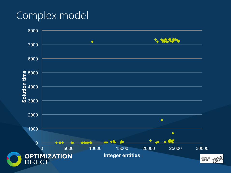
Complex model
0
1000
2000
3000
4000
5000
6000
7000
8000
0 5000 10000 15000 20000 25000 30000
Solu
tion
time
Integer entities
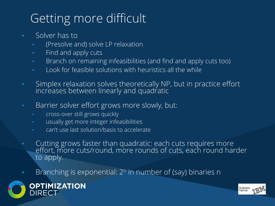
Getting more difficult • Solver has to
• (Presolve and) solve LP relaxation • Find and apply cuts • Branch on remaining infeasibilities (and find and apply cuts too) • Look for feasible solutions with heuristics all the while
• Simplex relaxation solves theoretically NP, but in practice effort increases between linearly and quadratic
• Barrier solver effort grows more slowly, but: • cross-over still grows quickly • usually get more integer infeasibilities • can’t use last solution/basis to accelerate
• Cutting grows faster than quadratic: each cuts requires more effort, more cuts/round, more rounds of cuts, each round harder to apply.
• Branching is exponential: 2n in number of (say) binaries n
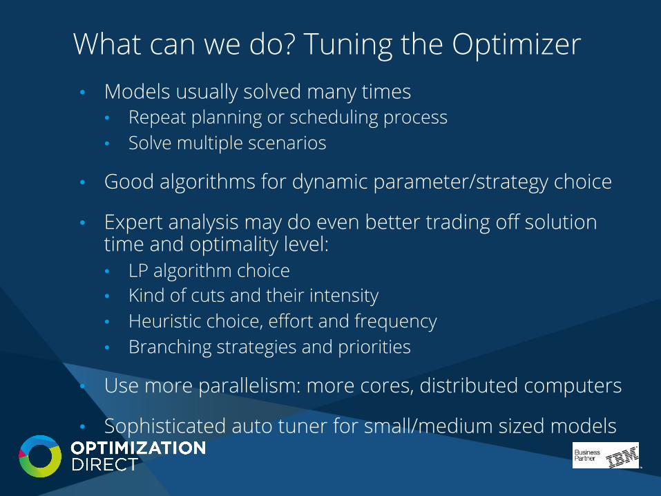
What can we do? Tuning the Optimizer • Models usually solved many times
• Repeat planning or scheduling process • Solve multiple scenarios
• Good algorithms for dynamic parameter/strategy choice
• Expert analysis may do even better trading off solution time and optimality level: • LP algorithm choice • Kind of cuts and their intensity • Heuristic choice, effort and frequency • Branching strategies and priorities
• Use more parallelism: more cores, distributed computers
• Sophisticated auto tuner for small/medium sized models
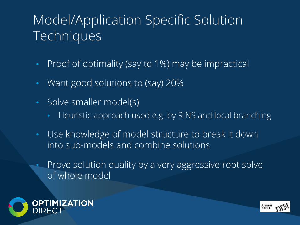
Model/Application Specific Solution Techniques
• Proof of optimality (say to 1%) may be impractical
• Want good solutions to (say) 20%
• Solve smaller model(s) • Heuristic approach used e.g. by RINS and local branching
• Use knowledge of model structure to break it down into sub-models and combine solutions
• Prove solution quality by a very aggressive root solve of whole model
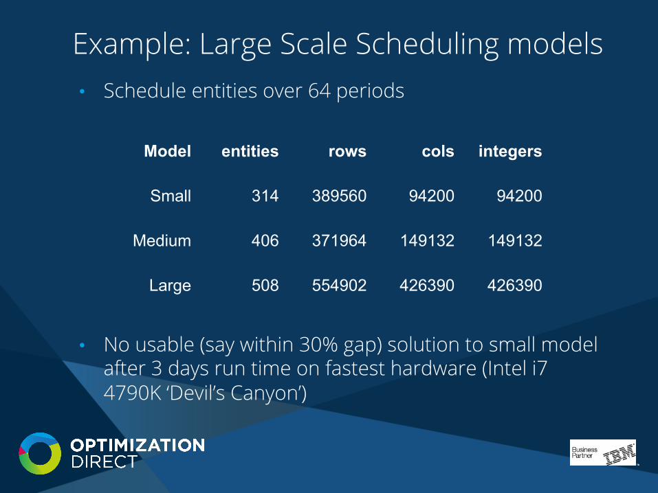
Example: Large Scale Scheduling models • Schedule entities over 64 periods
• No usable (say within 30% gap) solution to small model after 3 days run time on fastest hardware (Intel i7 4790K ‘Devil’s Canyon’)
Model entities rows cols integers
Small 314 389560 94200 94200
Medium 406 371964 149132 149132
Large 508 554902 426390 426390

Heuristic Solution Approach
• Solves sequence of sub-models
• Delivers usable solutions (12%-16% gap)
• Takes 4-36 hours run time
• Multiple instances can be run concurrently with different seeds
• Can run on only one core
• Can interrupt at any point and take best solution so far time limit / call-back /SIGINT

Heuristic Results on Scheduling Models Seed Solu(on Time Gap
Small 1234 118 65818 15.2% 5678 118 41122 15.2% 9012 117 38243 14.5% 21098 117 27623 14.5%
Medium 1234 703.32 100000 5678 728.64 100000 9012 718.23 100000 21098 832.43 100000
Large 1234 1039.67 60000 5678 1039.47 60000 9012 1039.43 60000 21098 1044.09 60000
Best bound of 100 established by separate CPLEX run Times are in seconds on Intel i7-‐4790K @ 4.4GHz (1 core)
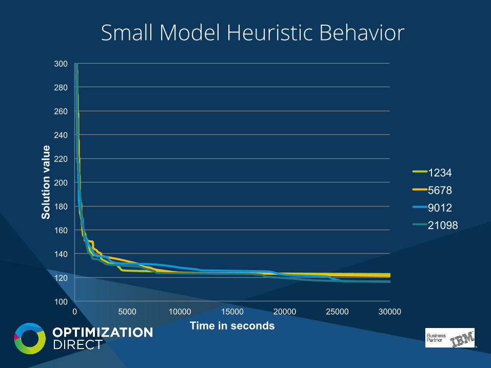
Small Model Heuristic Behavior
100
120
140
160
180
200
220
240
260
280
300
0 5000 10000 15000 20000 25000 30000
Solu
tion
valu
e
Time in seconds
1234 5678 9012 21098

Medium Model Heuristic Behavior
500
700
900
1100
1300
1500
1700
1900
0 20000 40000 60000 80000 100000 120000 140000 160000
Solu
tion
valu
e
Time in seconds
1234 5678 9012 21098

Large Model Heuristic Behavior
1020
1040
1060
1080
1100
1120
1140
1160
1180
0 10000 20000 30000 40000 50000 60000 70000
Solu
tion
valu
e
Time in seconds
1234
5678
9012
21098

Parallel Heuristic Approach
• Run several heuristic threads with different seeds simultaneously
• CPLEX callable library very flexible, so • Exchange solution information between runs • Kill sub-model solves when done better elsewhere
• Improves sub-model selection
• 4 instances run on 4 core i7-4790K • Each heuristic thread run with single CPLEX thread
i.e. 1 core each • Compare with serial runs using a single CPLEX thread
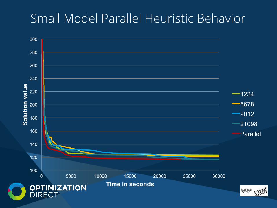
Small Model Parallel Heuristic Behavior
100
120
140
160
180
200
220
240
260
280
300
0 5000 10000 15000 20000 25000 30000
Solu
tion
valu
e
Time in seconds
1234 5678 9012 21098 Parallel

Medium Model Parallel Heuristic Behavior
500
700
900
1100
1300
1500
1700
1900
0 20000 40000 60000 80000 100000 120000 140000 160000
Solu
tion
valu
e
Time in seconds
1234 5678 9012 21098 Parallel

Large Model Parallel Heuristic Behavior
1020
1040
1060
1080
1100
1120
1140
1160
1180
0 10000 20000 30000 40000 50000 60000 70000
Solu
tion
valu
e
Time in seconds
1234
5678
9012
21098
Parallel
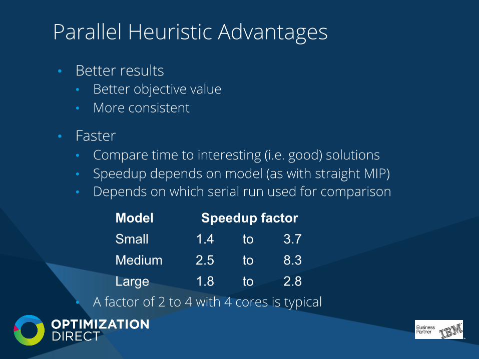
Parallel Heuristic Advantages
• Better results • Better objective value • More consistent
• Faster • Compare time to interesting (i.e. good) solutions • Speedup depends on model (as with straight MIP) • Depends on which serial run used for comparison
• A factor of 2 to 4 with 4 cores is typical
Model Speedup factor Small 1.4 to 3.7 Medium 2.5 to 8.3 Large 1.8 to 2.8