cpe 619 workloads: types, selection, characterization aleksandar milenković the lacasa laboratory...

CPE 619Workloads:

Types, Selection, Characterization

Aleksandar Milenković

The LaCASA Laboratory

Electrical and Computer Engineering Department

The University of Alabama in Huntsville

http://www.ece.uah.edu/~milenka

http://www.ece.uah.edu/~lacasa

2

Part II: Measurement Techniques and Tools

Measurements are not to provide numbers but insight - Ingrid Bucher

Measure computer system performance Monitor the system that is being subjected to a

particular workload How to select appropriate workload

In general performance analysis should know1. What are the different types of workloads?2. Which workloads are commonly used by other analysts?3. How are the appropriate workload types selected?4. How is the measured workload data summarized?5. How is the system performance monitored?6. How can the desired workload be placed on the system in a

controlled manner?7. How are the results of the evaluation presented?

3

Types of Workloads

Test workload – denotes any workload used in performance study

Real workload – one observed on a system while being used Cannot be repeated (easily) May not even exist (proposed system)

Synthetic workload – similar characteristics to real workload Can be applied in a repeated manner Relatively easy to port; Relatively easy to modify without affecting operation No large real-world data files; No sensitive data May have built-in measurement capabilities

Benchmark == Workload Benchmarking is process of comparing

2+ systems with workloads

benchmark v. trans. To subject (a system) to a series of testsIn order to obtain prearranged results not available on Competitive systems. – S. Kelly-Bootle, The Devil’s DP Dictionary

4

Test Workloads for Computer Systems

Addition instructions Instruction mixes Kernels Synthetic programs Application benchmarks

5

Addition Instructions

Early computers had CPU as most expensive component System performance == Processor Performance CPUs supported few operations;

the most frequent one was addition Computer with faster addition instruction

performed better Run many addition operations as test workload Problem

More operations, not only addition Some more complicated than others

6

Instruction Mixes

Number and complexity of instructions increased Additions were no longer sufficient

Could measure instructions individually, but they are used in different amounts

=> Measure relative frequencies of various instructions on real systems

Use as weighting factors to get average instruction time Instruction mix – specification of various instructions coupled

with their usage frequency Use average instruction time to compare different processors Often use inverse of average instruction time

MIPS – Million Instructions Per Second FLOPS – Millions of Floating-Point Operations Per Second

Gibson mix: Developed by Jack C. Gibson in 1959 for IBM 704 systems

7

Example: Gibson Instruction Mix1. Load and Store 13.22. Fixed-Point Add/Sub 6.13. Compares 3.84. Branches 16.65. Float Add/Sub 6.96. Float Multiply 3.87. Float Divide 1.58. Fixed-Point Multiply 0.69. Fixed-Point Divide 0.210. Shifting 4.411. Logical And/Or 1.612. Instructions not using regs 5.313. Indexing 18.0

Total 100

1959,IBM 650IBM 704

8

Problems with Instruction Mixes

In modern systems, instruction time variable depending upon Addressing modes, cache hit rates, pipelining Interference with other devices during

processor-memory access Distribution of zeros in multiplier Times a conditional branch is taken

Mixes do not reflect special hardware such as page table lookups

Only represents speed of processor Bottleneck may be in other parts of system

9

Kernels

Pipelining, caching, address translation, … made computer instruction times highly variable Cannot use individual instructions in isolation

Instead, use higher level functions Kernel = the most frequent function (kernel = nucleus) Commonly used kernels: Sieve, Puzzle, Tree

Searching, Ackerman's Function, Matrix Inversion, and Sorting

Disadvantages Do not make use of I/O devices Ad-hoc selection of kernels

(not based on real measurements)

10

Synthetic Programs

Proliferation in computer systems, OS emerged, changes in applications No more processing-only apps, I/O became important

too Use simple exerciser loops

Make a number of service calls or I/O requests Compute average CPU time and elapsed time

for each service call Easy to port, distribute (Fortran, Pascal) First exerciser loop by Buchholz (1969)

Called it synthetic program May have built-in measurement capabilities

11

Example of Synthetic Workload Generation Program

Buchholz, 1969

12

Synthetic Programs

Advantages Quickly developed and given to different vendors No real data files Easily modified and ported to different systems Have built-in measurement capabilities Measurement process is automated Repeated easily on successive versions of the operating systems

Disadvantages Too small Do not make representative memory or disk references Mechanisms for page faults and disk cache may not be

adequately exercised CPU-I/O overlap may not be representative Not suitable for multi-user environments because loops may

create synchronizations, which may result in better or worse performance

13

Application Workloads

For special-purpose systems, may be able to run representative applications as measure of performance E.g.: airline reservation E.g.: banking

Make use of entire system (I/O, etc) Issues may be

Input parameters Multiuser

Only applicable when specific applications are targeted For a particular industry: Debit-Credit for Banks

14

Benchmarks

Benchmark = workload Kernels, synthetic programs, application-level

workloads are all called benchmarks Instruction mixes are not called benchrmarks

Some authors try to restrict the term benchmark only to a set of programs taken from real workloads

Benchmarking is the process of performance comparison of two or more systems by measurements

Workloads used in measurements are called benchmarks

15

Popular Benchmarks

Sieve Ackerman’s Function Whetstone Linpack Dhrystone Lawrence Livermore Loops SPEC Debit-card Benchmark TPC EMBS

16

Sieve (1 of 2)

Sieve of Eratosthenes (finds primes) Write down all numbers 1 to n Strike out multiples of k for k = 2, 3, 5 … sqrt(n)

In steps of remaining numbers

17

Sieve (2 of 2)

18

Ackermann’s Function (1 of 2)

Assess efficiency of procedure calling mechanisms Ackermann’s Function has two parameters,

and it is defined recursively Benchmark is to call Ackerman(3,n)

for values of n = 1 to 6 Average execution time per call, the number of

instructions executed, and the amount of stack space required for each call are used to compare various systems

Return value is 2n+3-3, can be used to verify implementation

Number of calls:(512x4n-1 – 15x2n+3 + 9n + 37)/3

Can be used to compute time per call Depth is 2n+3 – 4, stack space doubles when n++

19

Ackermann’s Function (2 of 2)

(Simula)

20

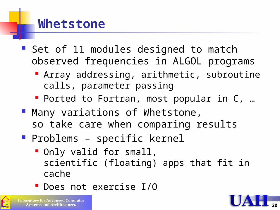
Whetstone

Set of 11 modules designed to match observed frequencies in ALGOL programs Array addressing, arithmetic, subroutine calls,

parameter passing Ported to Fortran, most popular in C, …

Many variations of Whetstone, so take care when comparing results

Problems – specific kernel Only valid for small,

scientific (floating) apps that fit in cache Does not exercise I/O

21

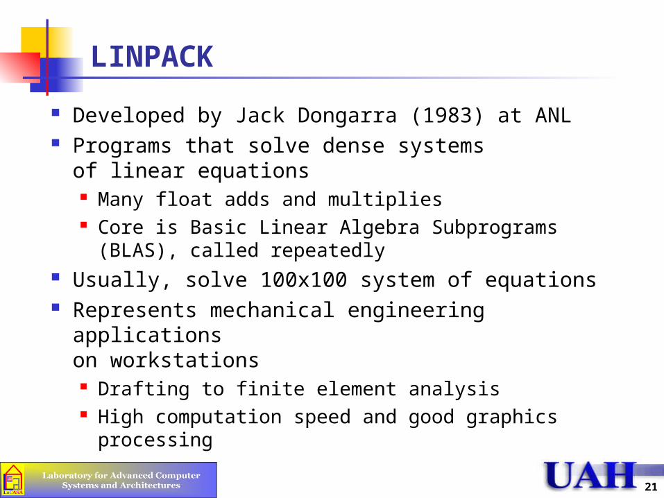
LINPACK

Developed by Jack Dongarra (1983) at ANL Programs that solve dense systems

of linear equations Many float adds and multiplies Core is Basic Linear Algebra Subprograms (BLAS),

called repeatedly Usually, solve 100x100 system of equations Represents mechanical engineering applications

on workstations Drafting to finite element analysis High computation speed and good graphics processing

22

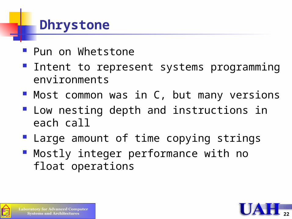
Dhrystone

Pun on Whetstone Intent to represent systems programming

environments Most common was in C, but many versions Low nesting depth and instructions in each call Large amount of time copying strings Mostly integer performance with no float operations

23

Lawrence Livermore Loops

24 vectorizable, scientific tests Floating point operations

Physics and chemistry apps spend about 40-60% of execution time performing floating point operations

Relevant for: fluid dynamics, airplane design, weather modeling

24

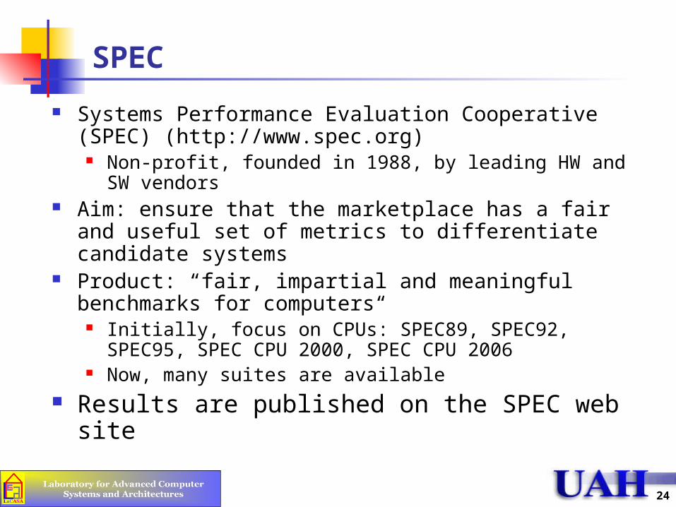
SPEC

Systems Performance Evaluation Cooperative (SPEC) (http://www.spec.org)

Non-profit, founded in 1988, by leading HW and SW vendors Aim: ensure that the marketplace has a fair and useful set of

metrics to differentiate candidate systems Product: “fair, impartial and meaningful benchmarks for

computers“ Initially, focus on CPUs: SPEC89, SPEC92, SPEC95, SPEC CPU

2000, SPEC CPU 2006 Now, many suites are available

Results are published on the SPEC web site

25

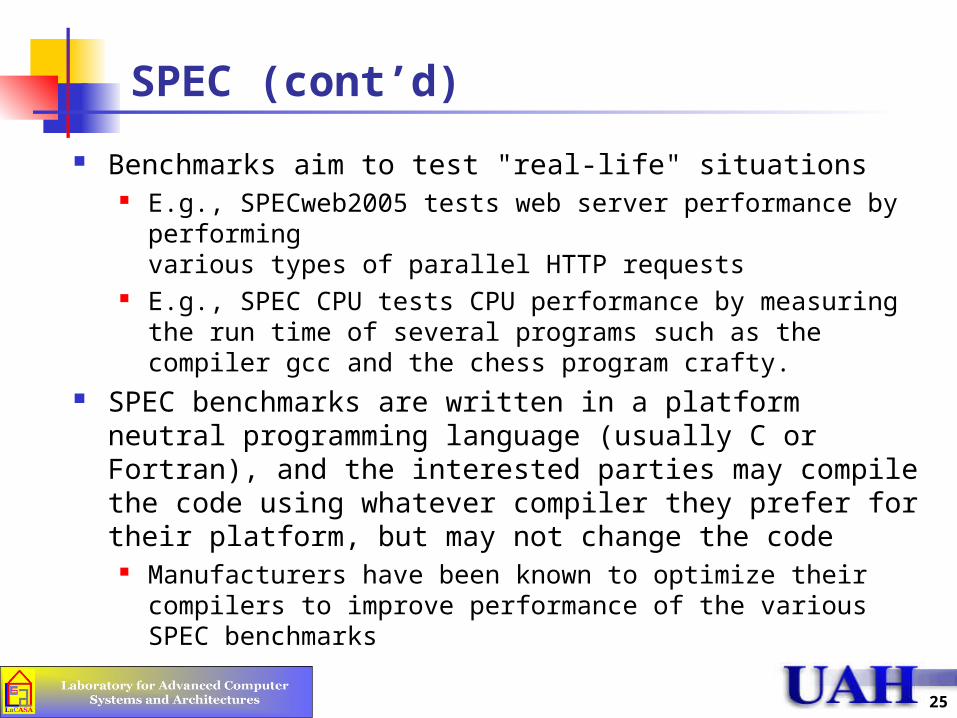
SPEC (cont’d)

Benchmarks aim to test "real-life" situations E.g., SPECweb2005 tests web server performance by performing

various types of parallel HTTP requests E.g., SPEC CPU tests CPU performance by measuring the run

time of several programs such as the compiler gcc and the chess program crafty.

SPEC benchmarks are written in a platform neutral programming language (usually C or Fortran), and the interested parties may compile the code using whatever compiler they prefer for their platform, but may not change the code

Manufacturers have been known to optimize their compilers to improve performance of the various SPEC benchmarks

26

SPEC Benchmark Suits (Current)

SPEC CPU2006: combined performance of CPU, memory and compiler CINT2006 ("SPECint"): testing integer arithmetic, with programs such as compilers,

interpreters, word processors, chess programs etc. CFP2006 ("SPECfp"): testing floating point performance, with physical simulations, 3D

graphics, image processing, computational chemistry etc. SPECjms2007: Java Message Service performance SPECweb2005: PHP and/or JSP performance. SPECviewperf: performance of an OpenGL 3D graphics system, tested with various

rendering tasks from real applications SPECapc: performance of several 3D-intensive popular applications on a given system SPEC OMP V3.1: for evaluating performance of parallel systems using OpenMP

(http://www.openmp.org) applications. SPEC MPI2007: for evaluating performance of parallel systems using MPI (Message

Passing Interface) applications. SPECjvm98: performance of a java client system running a Java virtual machine SPECjAppServer2004: a multi-tier benchmark for measuring the performance of Java 2

Enterprise Edition (J2EE) technology-based application servers. SPECjbb2005: evaluates the performance of server side Java by emulating a three-tier

client/server system (with emphasis on the middle tier). SPEC MAIL2001: performance of a mail server, testing SMTP and POP protocols SPECpower_2008: evaluates the energy efficiency of server systems. SPEC SFS97_R1: NFS file server throughput and response time

27

SPEC CPU Benchmarks

28

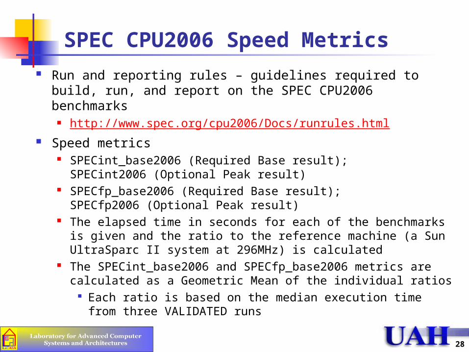
SPEC CPU2006 Speed Metrics

Run and reporting rules – guidelines required to build, run, and report on the SPEC CPU2006 benchmarks

http://www.spec.org/cpu2006/Docs/runrules.html Speed metrics

SPECint_base2006 (Required Base result); SPECint2006 (Optional Peak result)

SPECfp_base2006 (Required Base result); SPECfp2006 (Optional Peak result)

The elapsed time in seconds for each of the benchmarks is given and the ratio to the reference machine (a Sun UltraSparc II system at 296MHz) is calculated

The SPECint_base2006 and SPECfp_base2006 metrics are calculated as a Geometric Mean of the individual ratios

Each ratio is based on the median execution time from three VALIDATED runs

29

SPEC CPU2006 Throughput Metrics SPECint_rate_base2006 (Required Base result);

SPECint_rate2006 (Optional Peak result) SPECfp_rate_base2006 (Required Base result);

SPECfp_rate2006 (Optional Peak result) Select the number of concurrent copies of each benchmark to

be run (e.g. = #CPUs) The same number of copies must be used

for all benchmarks in a base test This is not true for the peak results where

the tester is free to select any combination of copies The "rate" calculated for each benchmark is a function of:

(the number of copies run * reference factor for the benchmark) / elapsed time in seconds which yields a rate in jobs/time.

The rate metrics are calculated as a geometric mean from the individual SPECrates using the median result from three runs

30

Debit-Credit (1/3)

Application-level benchmark Was de-facto standard for Transaction Processing

Systems Retail bank wanted 1000 branches, 10k tellers,

10,000k accounts online with peak load of 100 TPS Performance in TPS where 95% of all transactions

with 1 second or less of response time (arrival of last bit, sending of first bit)

Each TPS requires 10 branches, 100 tellers, and 100,000 accounts

System claiming 50 TPS performance should run: 500 branches; 5,000 tellers; 5,000,000 accounts

31

Debit-Credit (2/3)

32

Debit-Credit (3/3)

Metric: price/performance ratio Performance: Throughput in terms of TPS such that 95% of all

transactions provide one second or less response time Response time: Measured as the time interval between the

arrival of the last bit from the communications line and the sending of the first bit to the communications line

Cost = Total expenses for a five-year period on purchase, installation, and maintenance of the hardware and software in the machine room

Cost does not include expenditures for terminals, communications, application development, or operations

Pseudo-code Definition of Debit-Credit See Figure 4.5 in the book

33

TPC

Transaction Processing Council (TPC) Mission: create realistic and fair benchmarks for TP For more info: http://www.tpc.org

Benchmark types TPC-A (1985) TPC-C (1992) – complex query environment TPC-H – models ad-hoc decision support (unrelated queries, no

local history to optimize future queries) TPC-W – transaction Web benchmark (simulates the activities of

a business-oriented transactional Web server) TPC-App – application server and Web services benchmark

(simulates activities of a B2B transactional application server operating 24/7)

Metric: transaction per second, also include response time (throughput performance is measure only when response time requirements are met).

34

EMBS

Embedded Microprocessor Benchmark Consortium (EEMBC, pronounced “embassy”)

Non-profit consortium supported by member dues and license fees Real world benchmark software helps designers select the right

embedded processors for their systems Standard benchmarks and methodology ensure fair and reasonable

comparisons EEMBC Technology Center manages development of new benchmark

software and certifies benchmark test results For more info: http://www.eembc.com/

41 kernels used in different embedded applications Automotive/Industrial Consumer Digital Entertainment Java Networking Office Automation Telecommunications

The Art of Workload Selection

36

The Art of Workload Selection

Workload is the most crucial part of any performance evaluation Inappropriate workload will result in

misleading conclusions Major considerations in workload selection

Services exercised by the workload Level of detail Representativeness Timeliness

37

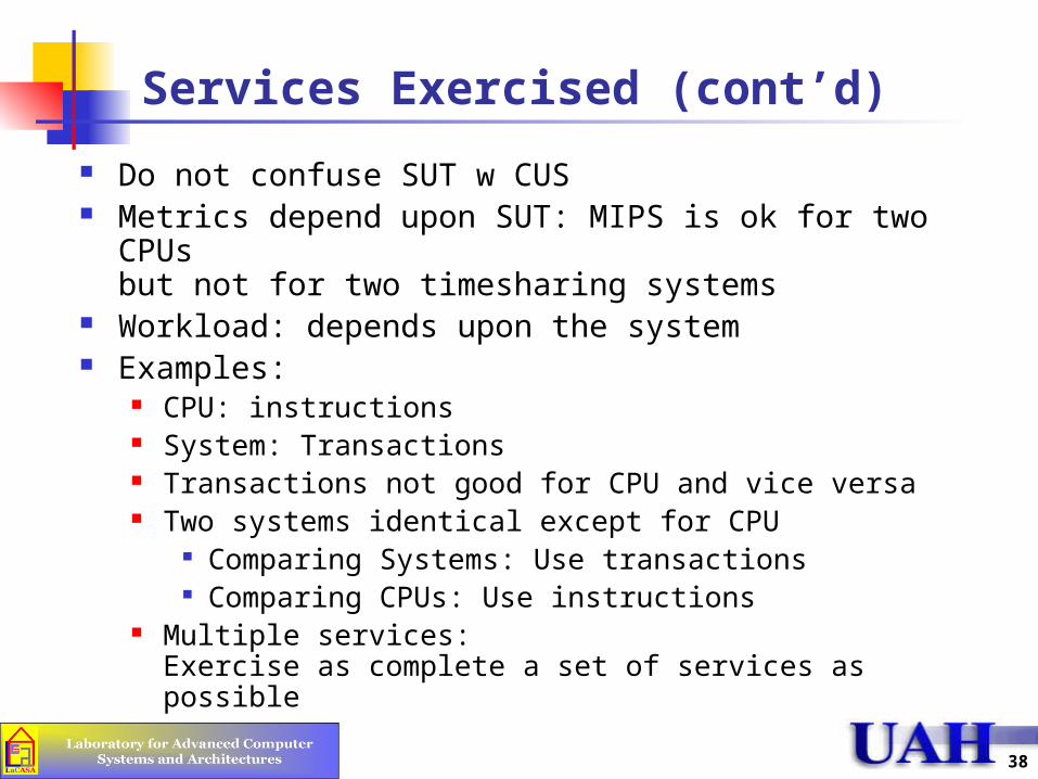
Services Exercised

SUT = System Under Test CUS = Component Under Study

38

Services Exercised (cont’d)

Do not confuse SUT w CUS Metrics depend upon SUT: MIPS is ok for two CPUs

but not for two timesharing systems Workload: depends upon the system Examples:

CPU: instructions System: Transactions Transactions not good for CPU and vice versa Two systems identical except for CPU

Comparing Systems: Use transactions Comparing CPUs: Use instructions

Multiple services: Exercise as complete a set of services as possible

39

Example: Timesharing Systems

Hierarchy of interfaces Applications

Application benchmark Operating System

Synthetic Program Central Processing Unit

Instruction Mixes Arithmetic Logical Unit

Addition instruction

40

Example: Networks

Application: user applications, such as mail, file transfer, http,… Workload: frequency of various types of applications

Presentation: data compression, security, … Workload: frequency of various types of security and

(de)compression requests Session: dialog between the user processes on the two end

systems (init., maintain, discon.) Workload: frequency and duration of various types of sessions

Transport: end-to-end aspects of communication between the source and the destination nodes (segmentation and reassembly of messages)

Workload: frequency, sizes, and other characteristics of various messages

Network: routes packets over a number of links Workload: the source-destination matrix, the distance, and

characteristics of packets Datalink: transmission of frames over a single link

Workload: characteristics of frames, length, arrival rates, … Physical: transmission of individual bits (or symbols) over the

physical medium Workload: frequency of various symbols and bit patterns

41

Example: Magnetic Tape Backup System

Backup System Services: Backup files, backup changed files, restore files, list

backed-up files Factors: File-system size, batch or background process,

incremental or full backups Metrics: Backup time, restore time Workload: A computer system with files to be backed up. Vary

frequency of backups Tape Data System

Services: Read/write to the tape, read tape label, auto load tapes Factors: Type of tape drive Metrics: Speed, reliability, time between failures Workload: A synthetic program generating representative tape I/O

requests

42

Magnetic Tape System (cont’d)

Tape Drives Services: Read record, write record, rewind, find record, move to

end of tape, move to beginning of tape Factors: Cartridge or reel tapes, drive size Metrics: Time for each type of service, for example, time to read

record and to write record, speed (requests/time), noise, power dissipation

Workload: A synthetic program exerciser generating various types of requests in a representative manner

Read/Write Subsystem Services: Read data, write data (as digital signals) Factors: Data-encoding technique, implementation technology

(CMOS, TTL, and so forth) Metrics: Coding density, I/O bandwidth (bits per second) Workload: Read/write data streams with varying patterns of bits

43

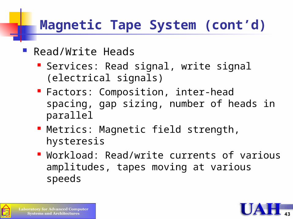
Magnetic Tape System (cont’d)

Read/Write Heads Services: Read signal, write signal (electrical signals) Factors: Composition, inter-head spacing, gap sizing,

number of heads in parallel Metrics: Magnetic field strength, hysteresis Workload: Read/write currents of various amplitudes,

tapes moving at various speeds

44

Level of Detail

Workload description varies from least detailed to a time-stamped list of all requests

1) Most frequent request Examples: Addition Instruction, Debit-Credit, Kernels Valid if one service is much more frequent than others

2) Frequency of request types List various services, their characteristics, and frequency Examples: Instruction mixes Context sensitivity

A service depends on the services required in the past => Use set of services (group individual service requests) E.g., caching is a history-sensitive mechanism

45

Level of Detail (Cont)

3) Time-stamped sequence of requests (trace) May be too detailed Not convenient for analytical modeling May require exact reproduction of component behavior

4) Average resource demand Used for analytical modeling Grouped similar services in classes

5) Distribution of resource demands Used if variance is large Used if the distribution impacts the performance

Workloads used in simulation and analytical modeling Non executable: Used in analytical/simulation modeling Executable: can be executed directly on a system

46

Representativeness

Workload should be representative of the real application

How do we define representativeness? The test workload and real workload should have

the same Arrival Rate: the arrival rate of requests should be the

same or proportional to that of the real application Resource Demands: the total demands on each of the

key resources should be the same or proportional to that of the application

Resource Usage Profile: relates to the sequence and the amounts in which different resources are used

47

Timeliness

Workloads should follow the changes in usage patterns in a timely fashion

Difficult to achieve: users are a moving target New systems new workloads Users tend to optimize the demand

Use those features that the system performs efficiently E.g., fast multiplication higher frequency of

multiplication instructions Important to monitor user behavior

on an ongoing basis

48

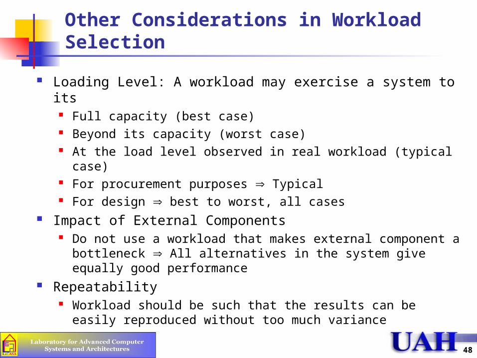
Other Considerations in Workload Selection

Loading Level: A workload may exercise a system to its Full capacity (best case) Beyond its capacity (worst case) At the load level observed in real workload (typical case) For procurement purposes Typical For design best to worst, all cases

Impact of External Components Do not use a workload that makes external component a

bottleneck All alternatives in the system give equally good performance

Repeatability Workload should be such that the results can be easily

reproduced without too much variance

49

Summary

Services exercised determine the workload Level of detail of the workload should match that of

the model being used Workload should be representative of the real

systems usage in recent past Loading level, impact of external components, and

repeatability or other criteria in workload selection

WorkloadCharacterization

51

Workload Characterization Techniques

Want to have repeatable workload so can compare systems under identical conditions

Hard to do in real-user environment Instead

Study real-user environment Observe key characteristics Develop workload model

Workload Characterization

Speed, quality, price. Pick any two. – James M. Wallace

52

Terminology

Assume system provides services User (workload component, workload unit) – entity

that makes service requests at the SUT interface Applications: mail, editing, programming .. Sites: workload at different organizations User Sessions: complete user sessions

from login to logout Workload parameters – the measure quantities,

service requests, resource demands used to model or characterize workload Ex: instructions, packet sizes, source or destination

of packets, page reference pattern, …

53

Choosing Parameters

The workload component should be at the SUT interface. Each component should represent as homogeneous a group

as possible. Combining very different users into a site workload may not be meaningful.

Better to pick parameters that depend upon workload and not upon system

Ex: response time of email not good Depends upon system

Ex: email size is good Depends upon workload

Several characteristics that are of interest Arrival time, duration, quantity of resources demanded

Ex: network packet size Have significant impact (exclude if little impact)

Ex: type of Ethernet card

54

Techniques for Workload Characterization

Averaging Specifying dispersion Single-parameter histograms Multi-parameter histograms Principal-component analysis Markov models Clustering

55

Averaging

Mean

Standard deviation:

Coefficient Of Variation:

Mode (for categorical variables): Most frequent value

Median: 50-percentile

s=¹x

56

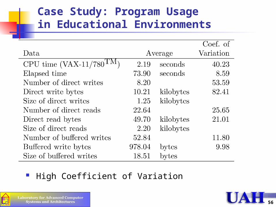
Case Study: Program Usage in Educational Environments

High Coefficient of Variation

57

Characteristics of an Average Editing Session

Reasonable variation

58



59

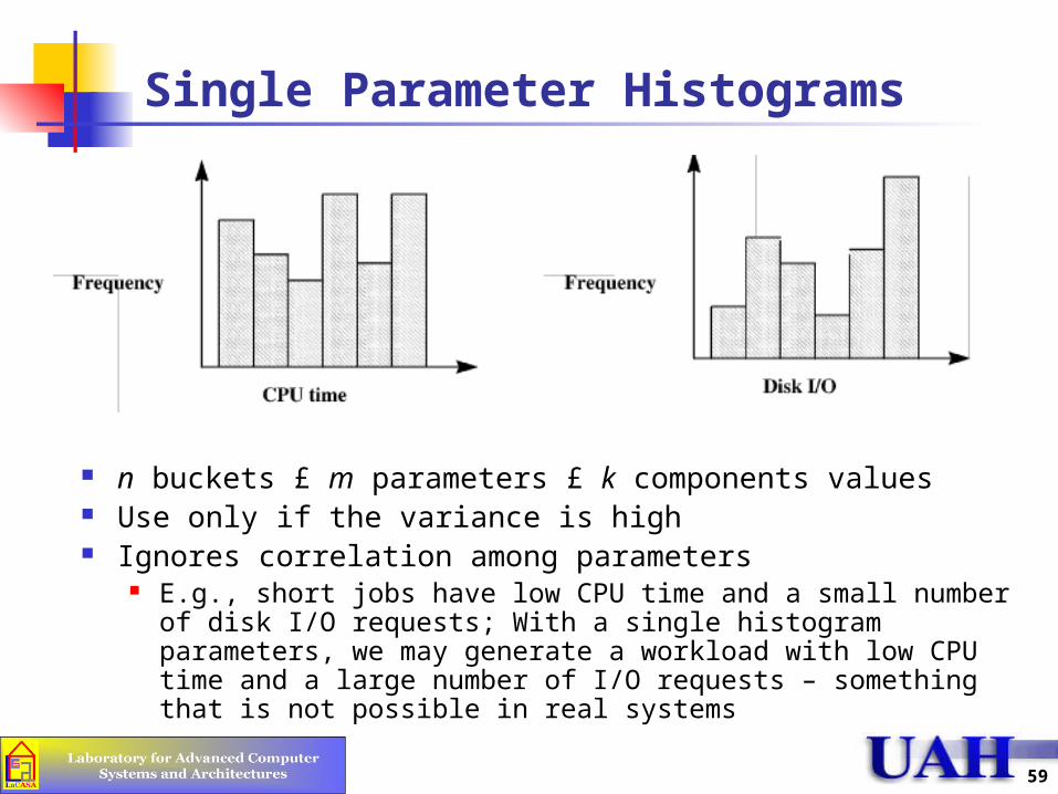
Single Parameter Histograms

n buckets £ m parameters £ k components values Use only if the variance is high Ignores correlation among parameters

E.g., short jobs have low CPU time and a small number of disk I/O requests; With a single histogram parameters, we may generate a workload with low CPU time and a large number of I/O requests – something that is not possible in real systems

60

Multi-parameter Histograms

Difficult to plot joint histograms for more than two parameters

61



62

Principal-Component Analysis

Goal is to reduce number of factors PCA transforms a number of (possibly) correlated

variables into a (smaller) number of uncorrelated variables called principal components

63

Principal Component Analysis (cont’d)

Key Idea: Use a weighted sum of parameters to classify the components

Let xij denote the ith parameter for jth component

yj = i=1n wi xij

Principal component analysis assigns weights w i's such that yj's provide the maximum discrimination among the components

The quantity yj is called the principal factor The factors are ordered. First factor explains the

highest percentage of the variance

64


Given a set of n parameters {x1, x2, … xn},the PCA produces a set of factors {y1, y2, … yn} such that

1) The y's are linear combinations of x's:

yi = j=1n aij xj

Here, aij is called the loading of variable xj on factor yi. 2) The y's form an orthogonal set, that is,

their inner product is zero:

<yi, yj> = k aikakj = 0

This is equivalent to stating that yi's are uncorrelated to each other

3) The y's form an ordered set such that y1 explains the highest percentage of the variance in resource demands

65

Finding Principal Factors

Find the correlation matrix Find the eigen values of the matrix and sort them in

the order of decreasing magnitude Find corresponding eigen vectors

These give the required loadings

66

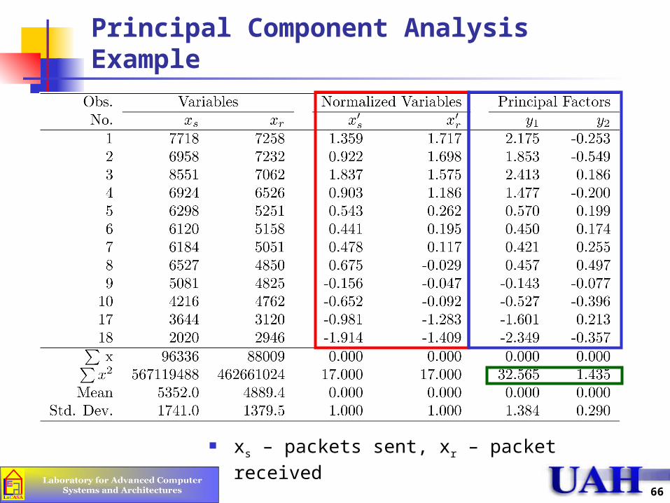
Principal Component Analysis Example

xs – packets sent, xr – packet received

67

Principal Component Analysis

1) Compute the mean and standard deviations of the variables:

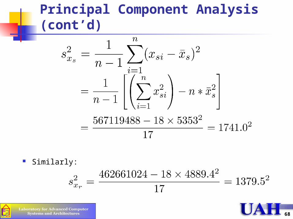
68


Similarly:

69


2) Normalize the variables to zero mean and unit standard deviation. The normalized values xs

’ and xr’ are given by:

70


3) Compute the correlation among the variables:

4) Prepare the correlation matrix:

71


5) Compute the eigenvalues of the correlation matrix: By solving the characteristic equation:

The eigenvalues are 1.916 and 0.084.

72


6) Compute the eigenvectors of the correlation matrix. The eigenvector q1 corresponding to 1=1.916 =1.916 are defined by the following relationship:

{C}{q}1 = 1 {q}1

or:

or:

q11=q21

73


Restricting the length of the eigenvectors to one:

7) Obtain principal factors by multiplying the eigen vectors by the normalized vectors:

74


8) Compute the values of the principal factors (last two columns)

9) Compute the sum and sum of squares of the principal factors The sum must be zero The sum of squares give the percentage of variation

explained

75


The first factor explains 32.565/(32.565+1.435) or 95.7% of the variation

The second factor explains only 4.3% of the variation and can, thus, be ignored

76



77

Markov Models

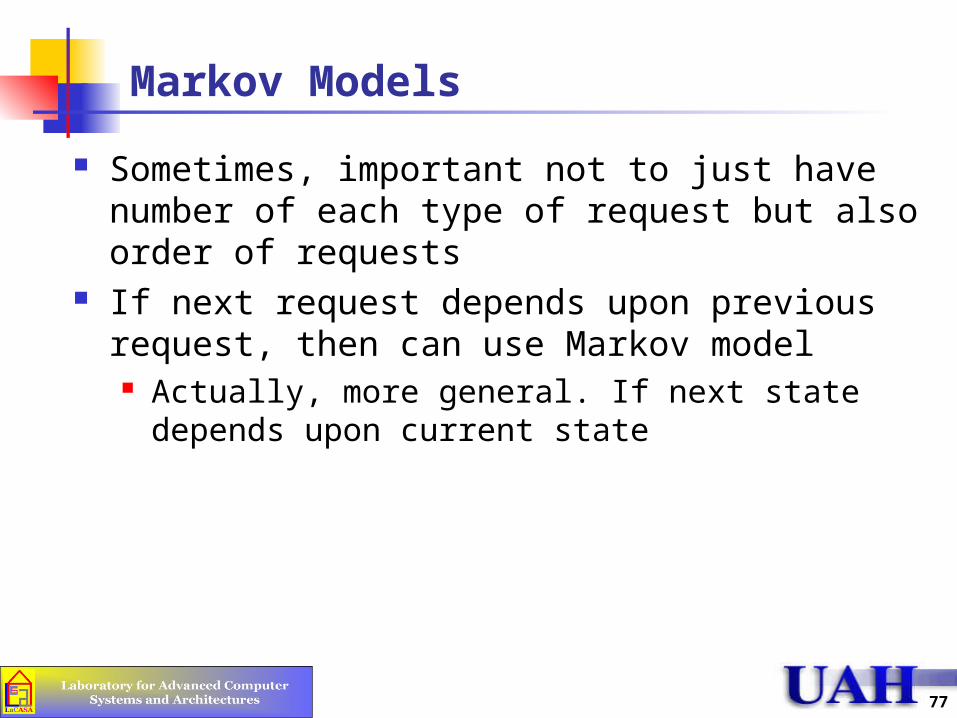
Sometimes, important not to just have number of each type of request but also order of requests

If next request depends upon previous request, then can use Markov model Actually, more general. If next state depends upon

current state

78

Markov Models (cont’d)

Example: process between CPU, disk, terminal

Transition matrices can be used also for application transitions E.g., P(Link|Compile)

Used to specify page-reference locality P(Reference module i | Referenced module j)

79

Transition Probability

Given the same relative frequency of requests of different types, it is possible to realize the frequency with several different transition matrices

Each matrix may result in a different performance of the system If order is important, measure the transition probabilities

directly on the real system Example: Two packet sizes: Small (80%), Large (20%)

80

Transition Probability (cont’d)

Option #1: An average of four small packets are followed by an average of one big packet, e.g., ssssbssssbssss.

Option #2: Eight small packets followed by two big packets, e.g., ssssssssbbssssssssbb

3) Generate a random number x; If x < 0.8, generate a small packet; otherwise generate a large packet

81



82

Clustering

May have large number of components Cluster such that components

within are similar to each other Then, can study one member

to represent component class Ex: 30 jobs with CPU + I/O. Five clusters.

Dis

k I/O

CPU Time

83

Clustering Steps

1. Take sample2. Select parameters3. Transform, if necessary4. Remove outliers5. Scale observations6. Select distance metric7. Perform clustering8. Interpret9. Change and repeat 3-710. Select representative components

84

1) Sampling

Usually too many components to do clustering analysis That’s why we are doing clustering

in the first place! Select small subset

If careful, will show similar behavior to the rest May choose randomly

However, if are interested in a specific aspect, may choose to cluster only “top consumers”

E.g., if interested in a disk, only do clustering analysis on components with high I/O

85

2) Parameter Selection

Many components have a large number of parameters (resource demands) Some important, some not Remove the ones that do not matter

Two key criteria: impact on perf & variance If have no impact, omit. If have little variance, omit.

Method: redo clustering with 1 less parameter. Count the number of components that change

cluster membership. If not many change, remove parameter

Principal component analysis: Identify parameters with the highest variance

86

3) Transformation

If distribution is skewed, may want to transform the measure of the parameter

Ex: one study measured CPU time Two programs taking 1 and 2 seconds are as different

as two programs taking 10 and 20 milliseconds

Take ratio of CPU time and not difference

(More in Chapter 15)

87

4) Outliers

Data points with extreme parameter values Can significantly affect max or min

(or mean or variance) For normalization (scaling, next) their

inclusion/exclusion may significantly affect outcome Only exclude if do not consume

significant portion of resources E.g., disk backup may make a number of disk I/O

requests, and should not be excluded if backup is done frequently (e.g., several times a day); may be excluded if done once in a month

88

5) Data Scaling

Final results depend upon relative ranges Typically scale so relative ranges equal Different ways of doing this

89

5) Data Scaling (cont’d)

Normalize to Zero Mean and Unit Variance:

Weights: xik

0 = wk xik

wk / relative importance or wk = 1/sk

Range Normalization Change from [xmin,k,xmax,k] to [0,1] :

Affected by outliers

90

5) Data Scaling (cont’d)

Percentile Normalization Scale so 95% of values between 0 and 1

Less sensitive to outliers

91

6) Distance Metric

Map each component to n-dimensional space and see which are close to each other

Euclidean Distance between two components {xi1, xi2, … xin} and {xj1, xj2, …, xjn}

Weighted Euclidean Distance Assign weights ak for n parameters Used if values not scaled or if significantly different in importance

92

6) Distance Metric (cont’d)

Chi-Square Distance Used in distribution fitting Need to use normalized or the relative sizes influence

chi-square distance measure

• Overall, Euclidean Distance is most commonly used

93

7) Clustering Techniques

Goal: Partition into groups so the members of a group are as similar as possible and different groups are as dissimilar as possible

Statistically, the intragroup variance should be as small as possible, and inter-group variance should be as large as possible Total Variance = Intra-group Variance + Inter-

group Variance

94

7) Clustering Techniques (cont’d)

Nonhierarchical techniques: Start with an arbitrary set of k clusters, Move members until the intra-group variance is minimum.

Hierarchical Techniques: Agglomerative: Start with n clusters and merge Divisive: Start with one cluster and divide.

Two popular techniques: Minimum spanning tree method (agglomerative) Centroid method (Divisive)

95

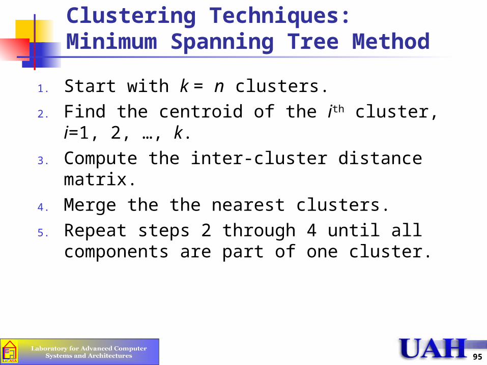
Clustering Techniques: Minimum Spanning Tree Method

1. Start with k = n clusters.

2. Find the centroid of the ith cluster, i=1, 2, …, k.

3. Compute the inter-cluster distance matrix.

4. Merge the the nearest clusters.

5. Repeat steps 2 through 4 until all components are part of one cluster.

96

Minimum Spanning Tree Example (1/5)

Workload with 5 components (programs), 2 parameters (CPU/IO) Measure CPU and I/O for each 5 programs

97

Minimum Spanning Tree Example(2/5)

Step 1): Consider 5 clusters with ith cluster having only ith program

Step 2): The centroids are {2,4}, {3,5}, {1,6}, {4,3} and {5,2}

1 2 43 5

12

43

5

Disk I/O

CPU Time

c

a

b

de

98


Step 3) Euclidean distance:

1 2 43 5

12

43

5

Disk I/O

CPU Time

c

a

b

de

Step 4) Minimum merge

99


The centroid of AB is {(2+3)/2, (4+5)/2}= {2.5, 4.5}. DE = {4.5, 2.5}

1 2 43 5

12

43

5

Disk I/O

CPU Time

c

a

b

dex

x

Minimum merge

100


Centroid ABC {(2+3+1)/3, (4+5+6)/3} = {2,5}

MinimumMergeStop

101

Representing Clustering

Spanning tree called a dendrogram Each branch is cluster, height where merges

12

43

5

a b c d e

Can obtain clustersfor any allowable distanceEx: at 3, get abc and de

102

Nearest Centroid Method

Start with k = 1. Find the centroid and intra-cluster variance for ith cluster,

i= 1, 2, …, k. Find the cluster with the highest variance and arbitrarily divide

it into two clusters Find the two components that are farthest apart, assign other

components according to their distance from these points. Place all components below the centroid in one cluster and all

components above this hyper plane in the other. Adjust the points in the two new clusters until the inter-cluster

distance between the two clusters is maximum Set k = k+1. Repeat steps 2 through 4 until k = n

103

Interpreting Clusters

Clusters will small populations may be discarded If use few resources If cluster with 1 component uses 50% of

resources, cannot discard! Name clusters, often by resource demands

Ex: “CPU bound” or “I/O bound” Select 1+ components from each cluster as a

test workload Can make number selected proportional to cluster

size, total resource demands or other

104

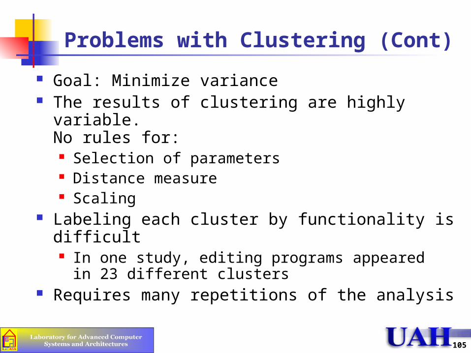
Problems with Clustering

105

Problems with Clustering (Cont)

Goal: Minimize variance The results of clustering are highly variable.

No rules for: Selection of parameters Distance measure Scaling

Labeling each cluster by functionality is difficult In one study, editing programs appeared

in 23 different clusters Requires many repetitions of the analysis

cpe 619 workloads: types, selection, characterization aleksandar milenković the lacasa laboratory...

Documents

workload benchmarking

particular workload

desired workload

appropriate workload

gibson instruction

test workload problem

measured workload data

addition computer