Comparing CFD and CORMIX for Buoyant Wastewater Near-Field Dispersion Modeling

Simon Mortensen1, Carl Jackson2, Ole Petersen3 and Geoff Wake4

1 DHI Water & Environment, Gold Coast, AUSTRALIA, email: sbm@dhigroup.com 2 DHI Water & Environment, Auckland, NEW ZEALAND.

3 DHI Water & Environment, Hørsholm, DENMARK. 4 Woodside Energy Ltd, Perth, AUSTRALIA.

The release plumes of Produced Formation Water (PFW) and Cooling Water from offshore oil and gas platforms have the potential to adversely impact the marine environment; therefore their effects need to be assessed and mitigated during engineering design. The near-field mixing processes of sub-surface strongly buoyant plumes, typically associated with PFW and Cooling Water, are complex and are poorly described in most commercially available software, thus making robust assessment of the potential impacts problematic. Consequently, Woodside Energy Ltd, as operator of the Browse Joint Venture, and DHI have carried out an investigation, in which a CFD model was used to perform a detailed 3D simulation of the near-field dispersion processes of a buoyant sub-surface plume. The CFD model was implemented in OpenFOAM® and included an extension of the standard “k-ε” turbulence model, adding a stratification term to the turbulence energy equation. In addition, the existing transport equations were extended to include dispersion of both temperature and salinity and a new boundary condition for temperature describing heat flux at the surface, based on Newton’s Law of Cooling, was also included. The computational domain captured the plume propagation out to 200 m from the outfall and utilized a cell subdivision method for splitting hexahedral, or cube-shaped, cells into nested sub-grids. This approach made it possible to capture very small turbulence structures close to the discharge point with length scales of only a few centimeters. Results for two selected release scenarios were compared to the industry-benchmark, empirically-based, plume-dispersion model, CORMIX. It was found that compared to the full CFD solution CORMIX underestimated the dilution occurring during the transition phase from a rising jet to a buoyant surface plume. It was also found that the CFD model was capable of reproducing a split in peak concentrations of the buoyant surface plume, which was attributed to a helical vortex generated through the interaction of the vertically aligned jet and the ambient side current. Keywords: 3D wastewater dispersion, buoyant plumes, CFD.

1. Introduction

The release plumes of Produced Formation Water (PFW) and Cooling Water from offshore oil and gas platforms have the potential to adversely impact the marine environment; therefore their effects need to be assessed and mitigated during engineering design. The near-field mixing processes of sub-surface strongly buoyant plumes, typically associated with PFW and Cooling Water, are complex and are poorly described in most commercially available software, thus making robust assessment of the potential impacts problematic. Consequently, Woodside Energy Ltd, as operator of the Browse Joint Venture, and DHI have carried out an investigation, in which a CFD model was used to

perform a detailed 3D simulation of the near-field dispersion processes of a buoyant sub-surface plume. In this paper a detailed CFD approach has been used to simulate the near field mixing processes for two release scenarios. Scenario 1 consisted of a PFW release discharged at a rate of 2500 m

3/day while Scenario 2 consisted of a cooling

water release with a discharge rate of 90,000 m

3/day. Both release scenarios took place at a

floating infield platform (FIP) located with the Browse LNG Field. The ambient flow conditions consisted of a 0.22 m/s steady current, a water temperature of 28 degrees and a salinity of 34 ppt. Each scenario utilized a single port downward facing diffuser design located at 10 meters below the sea surface. The port diameters for scenario 1

and 2 were 6’’ and 1.2 m respectively resulting in initial discharge velocities of 1.6 m/s and 0.9 m/s. The discharge temperature of the scenario 1

release was 98 C and a salinity of 7 ppt, while the

scenario 2 release temperatures was 45 C and an salinity equaling the ambient (34 ppt). The scenario 1 PFW release was considered as a conservative tracer with an initial concentration of 30 mg/L, while the 0.2 ppm concentration chlorine content in scenario 2 was modeled assuming a 1

st order decay

with a half-life of 20 minutes.

2. Methodology

2.1 Numerical Model Framework

The open-source CFD software platform

OpenFOAM® was used in this study. OpenFOAM®

makes use of the finite-volume discretisation

approach for fluid flow applications. For the

purposes of this study the standard buoyantBoussinesqPimpleFoam solver has been

extended in the following ways:

Addition of a salinity field and associated

transport equation;

Addition of a passive pollutant concentration

field and associated transport equation, which

incorporates a temporal, exponential-decay

term; and

Addition of a new transport model that

calculates the density and other seawater

properties as a function of salinity and

temperature as provided by El-Dessouky &

Ettouney (2002).

For this study a new “k-ε” turbulence model was

created by adding a stratification term to the

turbulence-energy equation as described in Rodi

(1984). A new boundary condition for temperature

to describe the heat flux at the surface, based on

Newton’s Law of Cooling, was also included.

The approach invokes the Boussinesq

approximation for handling the buoyancy effects,

which allows for the solution of the simplified

incompressible Reynolds-Averaged Navier-Stokes

equations by neglecting the density variation except

for a buoyancy term in the momentum equation.

Hence:

( ) (( ) ) ( ) (1)

Where:

= 3-component fluid velocity vector;

= kinematic pressure less the hydrostatic

pressure;

= molecular kinematic viscosity;

= turbulent kinematic viscosity, which is provided

by the turbulence model (see below); = 3-component gravitational acceleration;

= 3-component position vector; and

= kinematic density.

The effect of the variation in density is taken into

account in the final term on the right-hand-side of

the equation. The Boussinesq approximation

involves dividing the entire equations by a reference

density and assuming that the difference between

the actual density and the reference density is small

enough to be ignored. Hence the Boussinesq

approximation is valid in this context when:

| | (2)

The variable is calculated explicitly at each time

step using the values for temperature and salinity

from the previous time step.

The continuity equation is significantly simplified by

assuming the seawater can be treated as an

incompressible fluid. Hence:

(3)

The turbulence is assumed to be isotropic, which

allows the turbulence closure scheme to consist of just two variables, k (turbulence energy) and ε

(turbulent dissipation).

It is assumed that the heat dispersion is dominated

by turbulent diffusion.

The k-ε turbulence model was chosen for this

application due to its proven performance for free-

shear flows. It is presented here in its

incompressible form.

( ) ((

) )

( ) (4)

( ) ((

) )

( )

( ) (5)

Where = modulus of the mean rate-of-strain

tensor; and are empirically

determined constants given by Wilcox D. C. (1994).

The final term on the right-hand side of the

equations is the buoyancy term. The effect of the

turbulence is incorporated into the momentum

equation via the kinematic eddy viscosity, , defined as:

(6)

Where is an empirically determined constant

given by Wilcox D. C. (1994).

The linear transport equations for temperature, salinity and effluent are expressed by:

( ) ((

) ) (7)

( ) ((

) ) (8)

( ) ((

) ) (9)

Where = laminar Prandtl number, which

determines the ratio of the laminar temperature

diffusion rate to the laminar momentum diffusion

rate and is provided by a relation found in El-

Dessouky & Ettouney (2002) and = turbulent

Prandtl number, which determines the ratio of the

turbulent temperature diffusion rate to the turbulent

momentum diffusion rate and is set to a constant

value of 0.8 after Hinze (1959). is the laminar

Schmidt number, which determines the ratio of the

laminar salt diffusion rate to the laminar momentum

diffusion rate and is set to a constant value of

1000.0, which is an approximate value as laminar

diffusion in this study is negligible when compared

to the turbulent diffusion; and is the turbulent

Schmidt number, which determines the ratio of the

turbulent salt diffusion rate to the turbulent

momentum diffusion rate and is set to a constant

value of 0.8 after Hinze (1959). is the pollutant

exponential decay rate.

2.2 Domains and Boundary Conditions

Each computational domain extended from the

water surface to a sufficient water depth to avoid

artificial lid effects affecting the strongly buoyant

plumes. Due to the transversal symmetry of the flow

problem and the assumption of isotropic turbulence,

only half of the domain is included in the

computational domain as illustrated in Figure 2-1. A

symmetry boundary condition is used in the plane of

the outlet pipe.

The geometrical dimensions for the two release

scenarios are presented in Table 2.1.

Table 2.1 Geometrical Dimensions of Computational Domains for Scenarios 1 and 2

Dimensions Scenario 1 Scenario 2

Pipe Diameter 0.1524 m 1.2 m

Length (in current direction) 220.0 m 220.0 m

Width 50.0 m 100.0 m

Depth 14.0 m 34.0 m

Figure 2-1 Scenario 2 domain (black outline), computational domain (transparent blue volume), pipe location (red cylinder indicated by red arrow), ambient current direction (blue arrows) and boundary names.

In order to achieve high spatial resolution in the

vicinity of the pipe outlet as well as allow for a

relatively large model domain, a flexible grid

solution was adopted to allow simulations to

complete in a timely fashion. OpenFOAM®’s snappyHexMesh has been employed to realised a

nested-cell approach. The mesh discretization

approach uses a cell subdivision method for splitting

hexahedral, or cube-shaped, cells repeated until a

user-specified size is reached. As the number of

cells increases by a factor of 8 at every level of

subdivision, the refinement must be carefully

targeted to the region of the plume. Figure 2-2 gives

an example of the nesting of computational cells

around the pipe and outlet for Scenario 1. The

largest cells in the figure have side lengths of 0.5 m

and the smallest have side lengths of 15.6 mm

corresponding to 1/10 of the pipe diameter. A

similar requirement of 10 cells across the width of

the pipe has been fulfilled in the Scenario 2

computational grid. The cell counts for all

computational grids, both for simulation 1 and 2, are

between 2 and 3 million cells.

Figure 2-2 the illustration shows an oblique view of the nested hexahedral computational cells for Scenario 1. Computational cell extents are shown in white. The largest cells shown have a side length of 0.5 m and the smallest have a size length of 15.6 mm.

The pollutant concentration is fixed at 1.0 at the

outlet in order to simplify calculations of relative

concentration and dilution. For Scenario 1, the

pollutant is a hydrocarbon with a concentration of 30

mg/L and for Scenario 2 the pollutant is chlorine

with a concentration of 0.2 ppm. To find the actual

concentration of the pollutant at any point in the

simulation results, the local, simulated concentration

need only be multiplied by the initial concentration.

Note that the decay rate of the chlorine is also

unaffected by using an initial concentration of 1.0 as

the half-life remains unchanged.

3. Results

The two simulations undertaken in this study were

continued until a steady state was achieved, which

required a simulated period of 1500 s for Scenario

1 and 2000 s for Scenario 2. In both cases the

minimum possible simulation period that allows full

flushing of the domain is 1000 s: domain length of

220 m and an ambient current of 0.22 m/s. The

results, discussed in this section are taken from

these steady-state solutions.

2.3 Qualitative Interpretation

In a qualitative sense, both buoyant jets behave in a similar manner, despite the differences in scale, refer to Table 2.1, and jet velocity at the outlet pipe. The jet at the outlet is directed vertically downwards and bends sharply, influenced by the ambient current as shown in Figure 3-1. Velocity vectors in the plane of each transverse slice indicate the development of a helical vortex. The rapid drop in pollutant concentration is also evident in the strong change in colouring of the transverse slices as the distance from the outlet increases (moving towards the foreground of the image).

Figure 3-1 Scenario 1 transverse slices coloured by relative pollutant concentration and indicative velocity direction arrows (shown in black). Outlet pipe shown in red and relative pollutant concentration 0.003 iso-surface plotted in yellow.

The development of the plume can be divided approximately into two stages: the rising-stage close to the outlet where the plume retains a jet-like shape and properties, shown in Figure 3-1; and the surface-stage where the plume is in contact with the surface and primarily spreads laterally, shown towards the top of Figure 3-2.

Figure 3-2 Aerial view of Scenario 1 plume shape defined by a pollutant dilution of 10000 sliced down the plane of symmetry and coloured by relative pollutant concentration. The approximate location where the plume reaches the surface is indicated at 30 m.

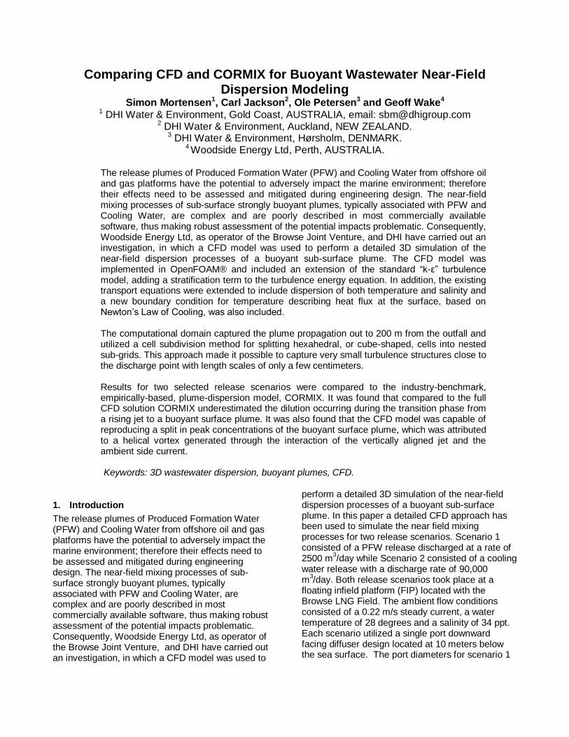
The distance from the outlet where the transition from the rising- to the surface-stage occurs in Scenario 1 has been approximated at 30 m, indicated by the dashed line in Figure 3-2. For Scenario 2, this transition occurs at approximately 40 m distance, indicated by the dashed line in Figure 3-3.

Figure 3-3 The figure presents an aaerial view of Scenario 2 plume shape defined by a pollutant dilution of 10000 sliced down the plane of symmetry and coloured by relative pollutant concentration. The approximate location where the plume reaches the surface is indicated at 40 m.

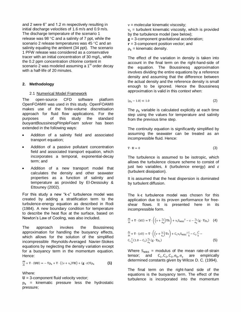
The rising-stage is characterised by strong turbulent mixing that results in a rapid increase in dilution, whereas the surface-stage is characterised by a more gentle increase in dilution as the buoyancy of the plume dominates and causes lateral spreading. Although a sharp transition from the rising-stage to the surface-stage makes simpler, conceptual models of the plume dynamics possible, the CFD results indicate that there is significant overlap between the two stages. In this transition-stage much of the strong turbulent mixing of the rising-stage is retained and slowly dissipates as the surface plume develops. The existence of this transition significantly increases the rate of dilution. The CFD results provide further evidence for a transition zone: rotational velocities, in the plane perpendicular to the ambient current direction, can be detected even 200 m downstream of the outlet as shown in Figure 3-4. The pair of helical vortices that originate at the outlet appear to influence the shape of the plume and play key roles in the lateral spreading of the surface-stage plume.

Figure 3-4 Scenario 2 transverse slices at 20-m intervals coloured by relative pollutant concentration and iso-surface of 0.0001. Location of maximum concentration indicated at 2 m intervals by white dots.

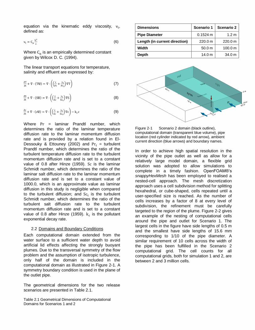
A very similar flow pattern develops in Scenario 2,

as shown in Figure 3-5 and Figure 3-6. There is a

more distinct shift in the location of the maximum

concentration, corresponding to minimum dilution

and indicated by white dots at 2 m intervals in

Figure 3-4, Figure 3-5 and Figure 3-6, in the

Scenario 2 results than in the Scenario 1 results.

Figure 3-5 Scenario 2 transverse slices at 20-m intervals coloured by relative pollutant concentration and contour of 0.0001. Location of maximum concentration indicated at 2 m intervals by white dots.

The reason for the shift in location of the maximum concentration is most clearly visible in Figure 3-6: effluent concentration is fed to the surface by the sub-surface vortex and then the maximum concentration at the centre of the sub-surface vortex decays at a faster rate than the concentration at the surface. The observed pattern in the surface-stage agrees well with other investigations (Petersen, 1992)

Figure 3-6 Four Scenario 2 transverse slices at 20-m intervals coloured by relative pollutant concentration and iso-surface of 0.0001. Location of maximum concentration indicated at 2 m intervals by white dots.

2.4 Comparison with CORMIX

In order to compare the CFD results with the CORMIX output for the two scenarios, integral values were extracted from the CFD results. CORMIX produces estimates of mean concentration and maximum concentration at distances downstream of the outlet for the rising-stage, but only produces mean concentration estimates for the surface-stage. This is a result of completely different mathematical treatments used by CORMIX for the different stages of the plume. Corresponding values of mean and maximum concentration were extracted from transverse slices of the CFD results at 2 m intervals as depicted in Figure 3-7.

Figure 3-7 Scenario 1 domain with transverse slices, at 2 m intervals, used in the results processing coloured by relative pollutant concentration. Outlet pipe location indicated by red arrow, ambient current direction indicated by blue arrow and boundary names shown (where boundary is visible).

The extraction of the maximum concentration at each transverse slices is straightforward, however mean concentration requires the definition of the area over which to perform the integration. In this study, the area is defined at each transverse slice by a contour line corresponding to a percentile of the maximum concentration on that slice. Mean concentrations calculated using percentiles of 1 %, 5 % and 10 % have been reported, in order to demonstrate the sensitivity of this approach. Overall, this approach has proven to be robust. Table 3.1 and Table 3.2 present extracted integral values at 5 distances downstream of the outlet: 10 m, 25 m, 50 m, 100 m and 200 m for Scenario 1 and Scenario 2, respectively. Table 3.1 Scenario 1 relative pollutant concentrations at distances downstream of the outlet. CFD mean pollutant concentrations given for cut-off percentiles 1%, 5%, and 10%.

Relative Pollutant

Concentration (-)

Distance from the Outlet (m)

10 25 50 100 200

CF

D

Max. 0.0216 0.00799 0.00356 0.00173 0.00117

Mean (1%)

0.00849 0.00281 0.00147 0.000789 0.000477

Mean (5%)

0.00934 0.00319 0.00170 0.000907 0.000554

Mean (10%)

0.0101 0.00350 0.00185 0.000980 0.000591

CO

RM

IX

Max. 0.0104 - - - -

Mean 0.00610 0.00270 0.00239 0.00202 0.00178

For both scenarios the maximum and mean

concentration values predicted by CFD are greater

than those predicted by CORMIX for distances of 10

and 25 m. This trend reverses for distances of 50 m

and greater, where the concentrations predicted by

CORMIX are higher than those predicted by CFD.

Compared to CORMIX, the CFD simulations predict

less mixing in the rising-stage and more mixing in

the beginning of the surface-stage. Plots of mean

concentration for Scenario 1 are provided in Figure

3-8 and Figure 3-9 where the rising- and surface-

stage are presented separately due to vertical

scaling issues.

Table 3.2 Scenario 2 relative pollutant concentrations at distances downstream of the outlet.

CFD mean pollutant concentrations given for percentiles 1%, 5%, and 10%.

Relative Pollutant

Concentration (-)

Distance from the Outlet (m)

10 25 50 100 200

CF

D

Max. 0.205 0.0643 0.0313 0.0127 0.00618

Mean (1%)

0.0768 0.0271 0.0131 0.00649 0.00281

Mean (5%)

0.0905 0.0296 0.0141 0.00708 0.00317

Mean

(10%) 0.103 0.0315 0.0149 0.00743 0.00336

CO

RM

IX

Max. 0.1475 0.0425 - - -

Mean 0.0867 0.0250 0.0176 0.0151 0.0133

The diffusive processes described by the CFD model and CORMIX predict very similar rates of dilution in the rising-stage, as shown in Figure 3-8 for Scenario 1. Although the values do not match exactly, the similarity of the shapes of the plotted lines suggest that the same processes are being described in both models. The CFD predicts higher concentrations, therefore lower dilutions in this stage.

Figure 3-8 Scenario 1 results. Rising-stage mean relative concentration in the direction of flow: CFD plots calculated using percentiles of 1%, 5% and 10%, and CORMIX mean concentration. Initial concentration of pollutant is fixed at 1.0.

In the surface-stage, the CFD and CORMIX results do not agree as well as in the rising-stage. Figure 3-9 presents the concentrations in the surface-stage for Scenario 1. The CFD results predict more rapid dilution from 20 m to 150 m from the outlet. After

150 m the rates of dilution (slopes of the plotted lines) in the CORMIX and CFD results begin to resemble each other. It is assumed that at this point both models are describing a decay-like process as the buoyancy-dominated spreading process takes over.

Figure 3-9 Scenario 1 results. Surface-stage mean relative concentration in the direction of flow: CFD plots calculated using percentiles of 1%, 5% and 10%, and CORMIX mean concentration. Initial concentration of pollutant is fixed at 1.0.

For Scenario 2, a very similar set of differences

between the CFD and CORMIX results are evident.

Figure 3-10 and Figure 3-11 present the rising- and

surface-stage concentration plots for Scenario 2.

Increased rates of dilution are indicated in the CFD

concentration profiles even up to 200 m

downstream of the outlet.

Figure 3-10 Scenario 2 results. Rising-stage mean relative concentration in the direction of flow: CFD plots

calculated using percentiles of 1%, 5% and 10%, and CORMIX mean concentration. Initial concentration of pollutant is fixed at 1.0.

Figure 3-11 Scenario 2 results. Surface-stage mean relative concentration in the direction of flow: CFD plots calculated using percentiles of 1%, 5% and 10%, and CORMIX mean concentration. Initial concentration of pollutant is fixed at 1.0.

The CFD results agree reasonably well with the CORMIX results for mean concentrations in the rising-stage of the plumes in both scenarios. The CFD and CORMIX mean concentration values diverge in the downstream direction in the surface-stage. However, at a distance of 200 m the slopes of mean concentration are similar for both CORMIX and CFD, indicating that a similar spreading process dominates in both models. Figure 3-12 presents the mean dilution transformed by log for Scenario 1. This plot is difficult to interpret, however it allows the profile of dilution (inverse of concentration) to be plotted for the entire domain in an easy-to-read fashion. This plot clearly shows the abrupt change in slope of the CORMIX predictions in the area of the transition. The CFD profiles, in contrast, are smooth and suggest a more natural transition from the rising-stage to the surface-stage. The Scenario 2 plot shows a similar phenomenon, so it has not been included here.

Figure 3-12 Scenario 1 results. Log mean dilution in the direction of flow: CFD plots calculated using percentiles of 1%, 5% and 10%, and CORMIX mean concentration. Initial concentration of pollutant is fixed at 1.0.

2.5 Comment

In both scenarios studied, the dilutions predicted by CFD are many times greater than those predicted by CORMIX. It is indicated that the reason for this lies in the fact that the sub-surface mixing process, initiated in the rising-stage, continues to operate in a transition zone that prevails for a distance up to around 150 m from the outlet in Scenario 1 and even beyond 200 m from the outlet in Scenario 2. This transition zone mixing is not described in the CORMIX model. The rate of dilution is much greater for the rising-stage than for the surface-stage.

4. Conclusion

The results produced by CFD differ considerably from those produced by CORMIX, both in detail and volume. Integrated concentration values, providing a mean concentration estimate for the CFD results, are the primary means of comparison with CORMIX. Integral values have been extracted from the CFD results using transverse slices cut downstream of the pipe at distances between 1 m and 200 m at 2 m intervals. The mean concentration of the plume is sensitive to the procedure used in its determination. In particular, the definition of the region, in which the plume is contained, has alternative definitions. For the CFD results in this study the plume region is defined by a fixed percentile of the concentration. This approach has been chosen for its simplicity

and for its ability to capture the important tendencies in the CFD results. It has also proven to be reasonable robust to the choice of percentile. The mixing processes in the rising- and surface-stage of the plume development are different, and consequently CORMIX applies separate empirical descriptions of them. The plumes from both scenarios behave in a similar manner and, when compared to CORMIX, display the same pattern of predicting less dilution in the rising-stage and higher dilution in the far surface-stage of the plumes. Transition from the rising-stage to the surface-stage for both scenarios occurs over a few metres, according to CORMIX. The CFD results show this transition to occur over a distance of approximately 120 m for the Scenario 1 plume and over a distance of much more than 160 m for the Scenario 2 plume. The CFD results indicate that the transition zone may be defined as the region of the plume where a gradual change from rising-stage to surface-stage dilution processes occur and that a sudden switch between the two as described in the CORMIX model, may not be a realistic description. The rising-stage dilution process appears to continue to be significant a distance after the plume has reached the surface and has a significant impact on the final dilution. Further validation of the CFD approach is required before a firm and quantitative conclusion can be reached for the transition between the rising- and surface-stage for this type of plume. It is concluded, however, that for the present case a less conservative estimate of plume dispersion, than that provided by CORMIX, is indicated by the detailed CFD mode.

5. References

[1] Doneker, R.L. and G.H. Jirka (2007): "CORMIX User

Manual - A Hydrodynamic Mixing Zone Model and

Decision Support System for Pollutant Discharges into

Surface Waters", US Environmental Protection Agency,

EPA-823-K-07-001, December 2007.

[2] El-Dessouky, H.T and H.M. Ettouney (2002):

Fundamentals of Sea Water Desalination, Elsevier.

[3] UNESCO (1981): The Practical Salinity Scale 1978

and the International Equation of State of Seawater 1980.

UNESCO Technical Papers in Marine Science 36, 25pp.

[4] Rodi, W. (1984) Turbulence models and their

application in hydraulics. IAHR, State of then art review,

Delft, the Netherlands.

[5] Petersen, O. (1992). Application of turbulence models

for transport of dissolved pollutants and particles. Series

Paper 4, Hydraulics and Coastal Engineering Laboratory,

Dept. Civil Eng., Aalborg University, pp. 130.

[6] Hinze J. O. (1959) “Turbulence”. Mc Graw-Hill, 790

pp.

[7] Wilcox D. C. (1994) “Turbulence Modeling for CFD”.

DCW Industries, Inc. 5354 Palm Drive, La Cañada,

California 91011.