covers wp4 benchmark 1 - qucosa: startseite · covers wp4 benchmark 1 ... and 100 205 11.9 13.3 0.3...

COVERS WP4 Benchmark 1

Fracture mechanical analysis of a thermal shockscenario for a VVER-440 RPV

Authors:

Martin AbendrothEberhard Altstadt

Acknowledgement:

This work was supported by the European Commission within the FP6 projectCOVERS.

June 04, 2007

2 ABSTRACT FZR-474

Abstract

This paper describes the analytical work done by modelling and evaluating a thermal shockin a WWER-440 reactor pressure vessel due to an emergency case. An axial oriented semi-elliptical underclad/surface crack is assumed to be located in the core weld line. Three-dimensional finite element models are used to compute the global transient temperatureand stress-strain fields. By using a three-dimensional submodel, which includes the crack,the local crack stress-strain field is obtained. With a subsequent postprocessing using thej-integral technique the stress intensity factors KI along the crack front are obtained. Theresults for the underclad and surface crack are provided and compared, together with acritical discussion of the VERLIFE code.

FZR-474 CONTENTS 3

Contents

1 Introduction 4

2 Benchmark Definition 52.1 Detailed description of the problem . . . . . . . . . . . . . . . . . . . . . . 5

3 Numerical Methods 93.1 Geometric Modelling . . . . . . . . . . . . . . . . . . . . . . . . . . . . . . 93.2 Submodel verification . . . . . . . . . . . . . . . . . . . . . . . . . . . . . . 163.3 Computation of stress intensity factors . . . . . . . . . . . . . . . . . . . . 18

3.3.1 The ANSYS kcalc method . . . . . . . . . . . . . . . . . . . . . . . 183.3.2 The VERLIFE method . . . . . . . . . . . . . . . . . . . . . . . . . 193.3.3 The j-integral method . . . . . . . . . . . . . . . . . . . . . . . . . 20

3.4 J-integral computation with ANSYS . . . . . . . . . . . . . . . . . . . . . 23

4 Results 254.1 Global model . . . . . . . . . . . . . . . . . . . . . . . . . . . . . . . . . . 254.2 Underclad crack . . . . . . . . . . . . . . . . . . . . . . . . . . . . . . . . . 294.3 Surface crack . . . . . . . . . . . . . . . . . . . . . . . . . . . . . . . . . . 31

5 Conclusions and Discussion 33

4 1 INTRODUCTION FZR-474

1 Introduction

The presented work is part of a benchmark from the workpackage four of the COVERSproject [1] within the Sixth Framework Programme of EURATOM. Aim of the COVERSproject is to ‘. . . establish a viable research and technical development structure with aview to change the scientific and technical cooperation of actors involved in WWER safetyresearch, in close co-operation with utilities, manufacturers, regulatory bodies and otherend users.’

One important point of workpackage four with the title ‘Material and EquipmentAgeing’ is ‘. . . to test and update the existing common unified procedure on plant lifeassessment VERLIFE. This document is prepared within FP5 with limited experience ofpractical use. It should be revised based on the:

• Available new information

• Experience gained during practical use

• Benchmark tests of different factors affecting the calculated service life according toVERLIFE’

The benchmark discussed here, refers to the chapter 5 of the VERLIFE code [6], whichdefines the assessment of component resistance against fast fracture. This assessmentis based on the stress intensity factors KI for a postulated crack. Especially, the coderecommends the j-integral to obtain the stress intensity factors. The well known j-integralintroduced by Eshelby [8], Cherepanov [7] and Rice [11] and modified by Shih at al. [12]is a measure for crack loading and directly related to the stress intensity factors. It hasbeen used by Bass at al. [3, 4], Kikuchi at al. [9] and Sievers and Hofler [13] to evaluatecracks in thermo-mechanical loaded pressure vessels.

FZR-474 2 BENCHMARK DEFINITION 5

2 Benchmark Definition

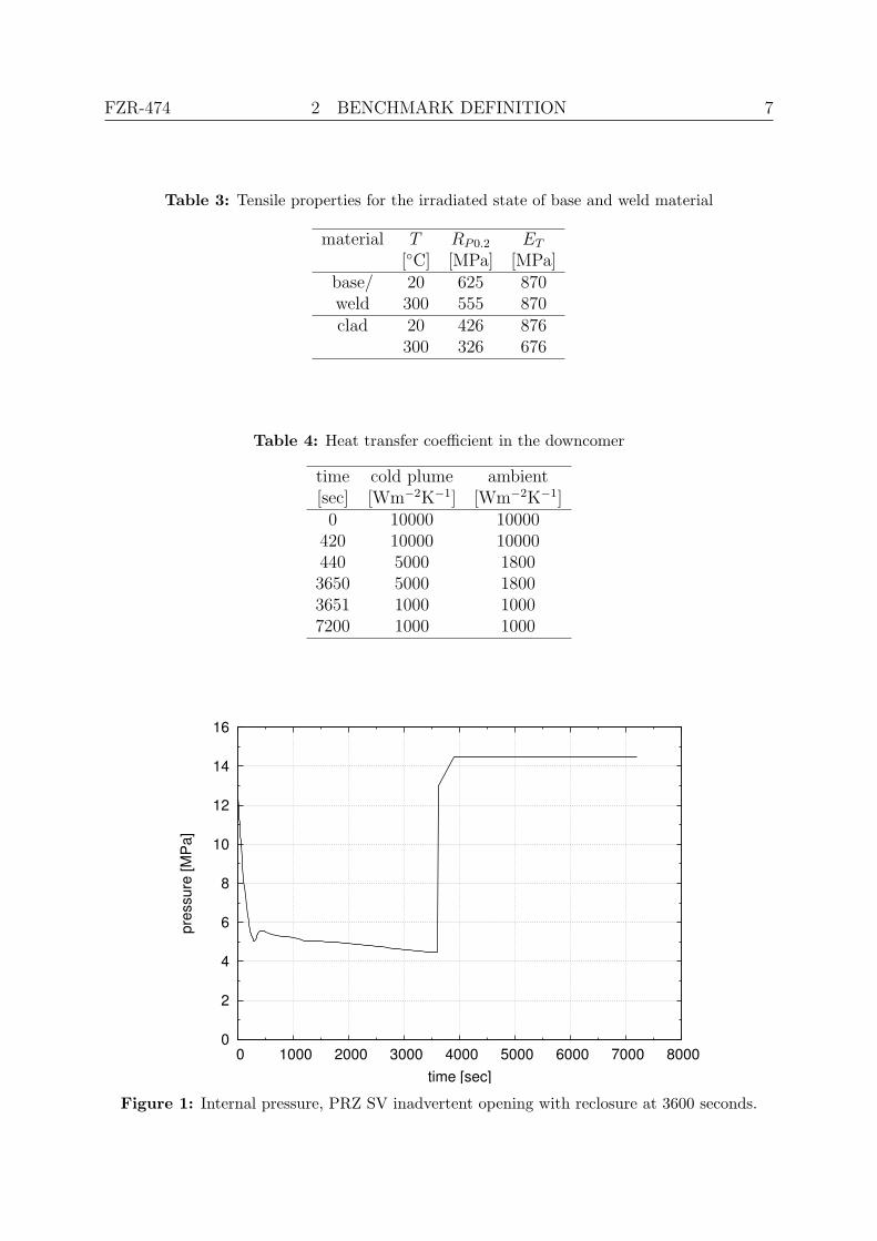
The given scenario describes a pressurized thermal shock (PTS) regime for a reactor pres-sure vessel (RPV) of the type WWER-440/V-213. The main reactor cooling system hasfailed and the emergency cooling system is the only source of cooling fluid. Additionally,an unintentional opening of a pressurizer safety valve (PRZ SV) is assumed, which will beclosed again after 3600 seconds. This scenario results in two opposite cold plumes belowthe cold legs in the downcomer of the RPV, which suddenly cool the inside of the RPV.The undercooled region includes the core weld line, which is supposed to be one of themost embrittled regions of the RPV due to neutron radiation. Additionally, weld linesare also likely locations for cracks or flaws. Therefore, the scenario postulates an axialoriented semi-elliptical underclad crack. The axial orientation is chosen because of themaximum principal stress in a pressurized cylindric vessel is acting in hoop direction andso perpendicular to the faces of the postulated crack. The undercooled inner surface ofthe RPV and the crack are exposed to tensile stress. Repressurizing the RPV after 3600seconds by closing the safety valve will suddenly increase the tensile stress and is assumedto be the critical phase of the scenario.

The primary questions regarding this scenario are:

• What is the loading of the crack during this scenario?

• What are the stress intensity factors during this scenario?

• What are the allowable stress intensity factors based on critical temperatures ofbrittleness Tk?

• What is the allowable critical temperature T ak of the material?

2.1 Detailed description of the problem

The component of interest is a WWER-440/V-213 RPV, which has an inner radius ofri = 1771 mm. The inner surface has a cladding with a thickness of sclad = 9 mm. Thethickness of the base material in the cylindric part of the vessel is sbase = 140 mm. Thegeometry of the two opposite cold plumes is given by means of levels, whereas level meansthe vertical distance below the lower part of the cold leg (see Fig. 3). Table 1 shows thefigures of the cold plumes. The geometry and the physical properties of the cold plumewere obtained from a thermohydraulic simulation, which is not part of this benchmark [10].

There is zero heat transfer at the outside of the vessel, which is reasonable because ofthe existence of an outer thermal isolation. The stress free temperature of the claddedvessel is Tsf = 267 ◦C. The weld material has the same thermal-physical and tensileproperties as the base material but is supposed to have residual stresses σR in both axialand circumferential orientation. These residual stresses result from the welding process.

σR = 60 MPa · cos

(2πx

sbase

)(1)

Here, x is the radial coordinate starting from the interface of cladding and base materialto the outside of the vessel. The postulated semi-elliptical underclad crack is located at

6 2 BENCHMARK DEFINITION FZR-474

the core weld 5/6 at level 3.485m. As already mentioned above, this weld accumulatesthe highest damage (embrittlement) due to neutron radiation of all welds from the RPVand is therefore the most critical one, which means that the ductile to brittle transitiontemperature (DBTT) for this weld line is above the DBTT for all the others.

The supposed crack width is a = 15 mm and the width/length ratio is a/c = 0.3.The crack is orientated in axial direction. The temperature dependent allowable stressintensity is given according to the VERLIFE code [6] Chapter 5.6 as:

[KIC ]3 = 26 + 36 exp[0.02 (T − Tk)] (2)

with [KIC ]3max = 200 MPam0.5. T denotes the temperature at the crack tip and Tk thecritical temperature, obtained from the ductile-to-brittle transition temperature.

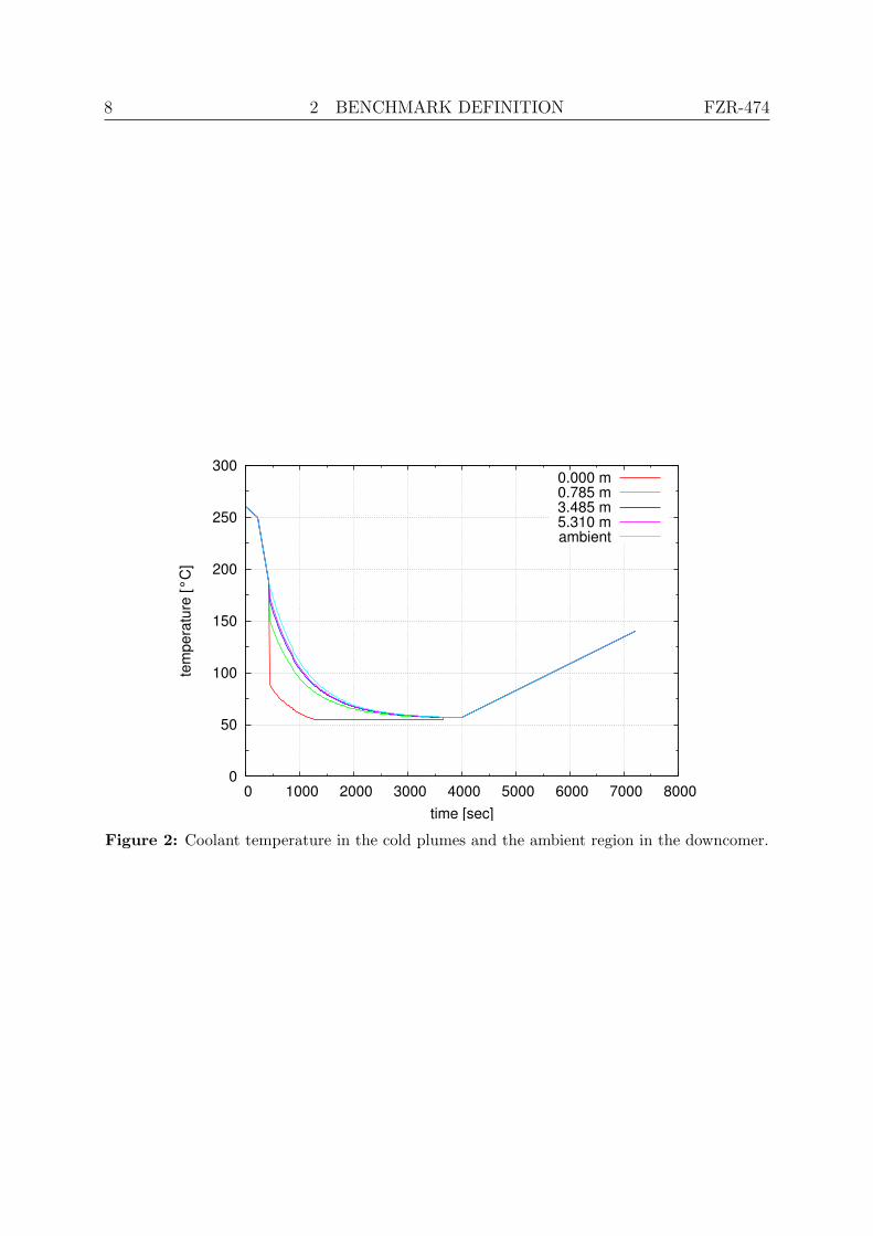
The tables 2 and 3 give the thermal-physical and tensile properties for the irradiatedstate of the base and the cladding material. In table 4 the heat transfer coefficient of thecold plum and the ambient region in the downcomer are given. Fig. 1 shows the internalpressure changing in time due to the opening and reclosure of the PRZ SV. In Fig. 2 thecoolant temperature in the downcomer is plotted over the time for the different levels.

Table 1: Cold plume geometry

level [m] width [m]0.000 0.80.785 0.83.485 1.8

> 3.485 1.8

Table 2: Thermal-physical properties of base and weld material [6], App. XV, T – temperature,E – elastic modulus, αref , α0 – thermal expansion coefficient based on reference andabsolute temperature, ν – Poisson ratio, λ – thermal conductivity, cp – specific heat,ρ – density

mat. T E αref α0 ν λ cp ρ

[◦C] [GPa] [10−6 K] [ - ][

Wm K

] [J

kg K

] [ kgm3

]base 20 210 - 12.9 0.3 35.9 445 7821and 100 205 11.9 13.3 0.3 37.3 477 7799weld 200 200 12.5 13.9 0.3 38.1 520 7771

300 195 13.1 14.5 0.3 37.3 562 7740clad 20 165 - 15.9 0.3 15.1 461 7900

100 160 14.6 16.5 0.3 16.3 494 7868200 153 15.7 16.5 0.3 17.6 515 7830300 146 16.0 16.8 0.3 18.8 536 7790

FZR-474 2 BENCHMARK DEFINITION 7

Table 3: Tensile properties for the irradiated state of base and weld material

material T RP0.2 ET

[◦C] [MPa] [MPa]base/ 20 625 870weld 300 555 870clad 20 426 876

300 326 676

Table 4: Heat transfer coefficient in the downcomer

time cold plume ambient[sec] [Wm−2K−1] [Wm−2K−1]

0 10000 10000420 10000 10000440 5000 18003650 5000 18003651 1000 10007200 1000 1000

0

2

4

6

8

10

12

14

16

0 1000 2000 3000 4000 5000 6000 7000 8000

pres

sure

[MPa

]

time [sec]Figure 1: Internal pressure, PRZ SV inadvertent opening with reclosure at 3600 seconds.

8 2 BENCHMARK DEFINITION FZR-474

0

50

100

150

200

250

300

0 1000 2000 3000 4000 5000 6000 7000 8000

tem

pera

ture

[°C]

time [sec]

0.000 m0.785 m3.485 m5.310 mambient

Figure 2: Coolant temperature in the cold plumes and the ambient region in the downcomer.

FZR-474 3 NUMERICAL METHODS 9

3 Numerical Methods

3.1 Geometric Modelling

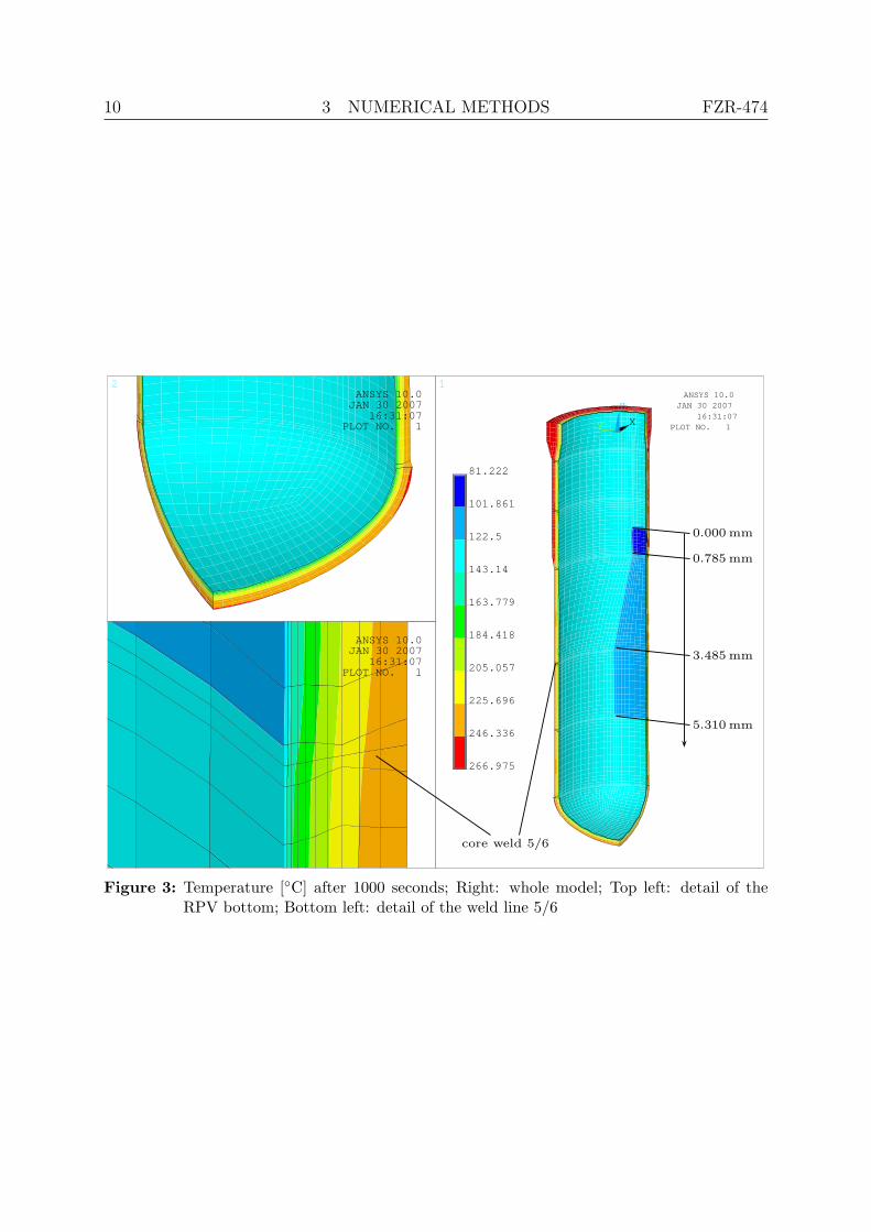
To solve the given problem we use a three-dimensional finite element (FE) model of onequarter of the RPV. Since the region of interest (core weld 5/6) is far away from the in-and outlets, these nozzles have been neglected in the model. This model does not containany crack so far. It is used to compute in a first run the transient spatial thermal field.

Fig. 3 shows the computed thermal field at the time t = 1000 s. On the right part ofthe figure the cold plume is clearly to see. The incoming cold water leads to a generalcool down of the inner surface of the RPV, but especially in the cold plum region thetemperatures are up to 50K lower than in the ambient region. This leads to elevatedtensile stresses in hoop and vertical direction in the cold plum region of the inner surfaceof the RPV.

In a second run the mechanical solution is obtained using the thermal field as a bodyload. In the mechanical solution also the time dependent inner pressure, the accelerationof gravity and the initial residual stresses in the welds are considered.

Fig. 4 shows the computed hoop stress at the time t = 1000 s. It can be seen that ingeneral the highest hoop stresses are located in the cladding which is directly in contactwith the coolant. Secondly, we identify the upper part, where the vessel wall thickness isgreater than in the lower part, having in general higher hoop stress values than the lowerpart. And thirdly, the cold plum region in the lower part is also a region with elevatedhoop stress.

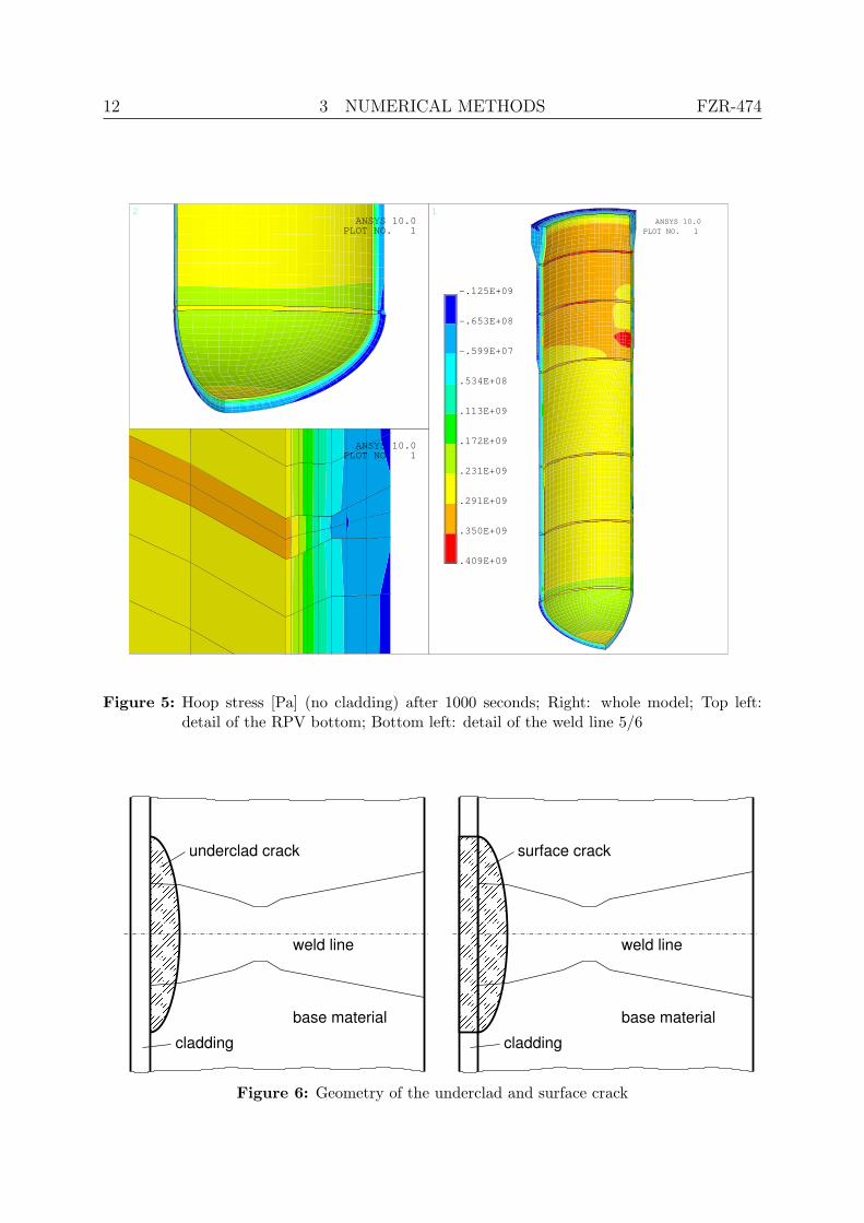
In Fig. 5 the cladding is virtually removed and we have a direct view to the base andweld material. It can be seen that the weld lines have higher hoop stress values than thebase material. This is due to the residual stresses, which are applied before the simulationstarts. With a closer look we find that the upper weld lines are subjected to higher hoopstresses, the reason for this is the greater RPV wall thickness. But we have to keep inmind that the upper weld lines are much less damaged due to radiation than the coreweld line.

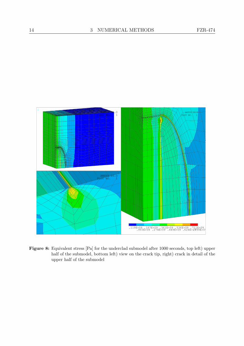
To consider cracks in the model we use a submodel technique. Two different crack areassumed, a underclad crack as defined in the benchmark and a surface crack as shownin Fig. 6. Only the crack and a reasonable large surrounding is modeled. At the cutboundaries of the submodel the interpolated degree of freedom results (displacements) ofthe global (coarse) model are applied. The thermal field obtained in the first run andthe gravity loads are used as a body loads. Additionally, the pressure (see Fig. 1) isapplied at the inner surface. Fig. 8 shows the equivalent stress in the submodel at timet = 1000 seconds. The crack is assumed to be an underclad crack. Here arises a principalproblem, since the cladding itself contains no crack and has common nodes with the basematerial, the crack mouth is virtually clamped close, which results in a second straightand sharp crackfront at the interface between cladding and base material.

The VERLIFE code does make any suggestions how to deal numerically with undercladcracks. Therefore a second submodel is used, which includes a surface crack which goesthrough the cladding. Fig. 9 shows the hoop stress at t = 1000 s. Here, the crack face isclearly distinguishable from the rest of the model.

10 3 NUMERICAL METHODS FZR-474

12

3

XY

Z

81.222

101.861

122.5

143.14

163.779

184.418

205.057

225.696

246.336

266.975

ANSYS 10.0JAN 30 2007

16:31:07PLOT NO. 1

ANSYS 10.0JAN 30 2007

16:31:07PLOT NO. 1

ANSYS 10.0JAN 30 2007

16:31:07PLOT NO. 1

0.000 mm

0.785 mm

3.485 mm

5.310 mm

core weld 5/6

Figure 3: Temperature [◦C] after 1000 seconds; Right: whole model; Top left: detail of theRPV bottom; Bottom left: detail of the weld line 5/6


12

3

-.125E+09

-.634E+08

-.215E+07

.591E+08

.120E+09

.182E+09

.243E+09

.304E+09

.365E+09

.427E+09

ANSYS 10.0PLOT NO. 1



Figure 4: Hoop stress [Pa] after 1000 seconds; Right: whole model; Top left: detail of the RPVbottom; Bottom left: detail of the weld line 5/6


12

3

-.125E+09

-.653E+08

-.599E+07

.534E+08

.113E+09

.172E+09

.231E+09

.291E+09

.350E+09

.409E+09




Figure 5: Hoop stress [Pa] (no cladding) after 1000 seconds; Right: whole model; Top left:detail of the RPV bottom; Bottom left: detail of the weld line 5/6

� � � � � ��

� � � � � ��

base materialcladding

weld line

underclad crack

� � � � � ��

� � � � � ��


weld line

surface crack

� ��

� ��

Figure 6: Geometry of the underclad and surface crack


12ANSYS 10.0

PLOT NO. 1ANSYS 10.0

PLOT NO. 1

P1

P2

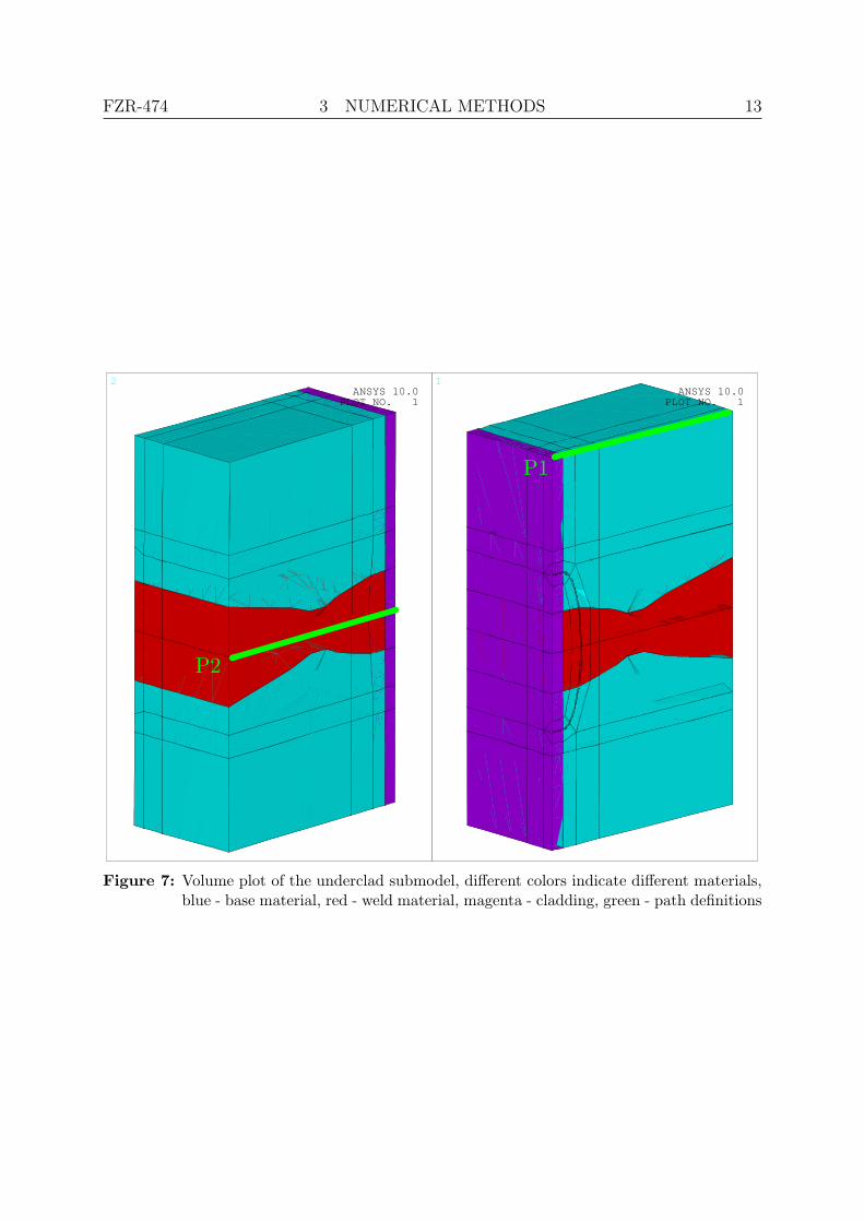
Figure 7: Volume plot of the underclad submodel, different colors indicate different materials,blue - base material, red - weld material, magenta - cladding, green - path definitions


12

3

.119E+08.993E+08

.187E+09.274E+09

.361E+09.449E+09

.536E+09.624E+09

.711E+09.799E+09




Figure 8: Equivalent stress [Pa] for the underclad submodel after 1000 seconds, top left) upperhalf of the submodel, bottom left) view on the crack tip, right) crack in detail of theupper half of the submodel


12

3

-.734E+08.128E+09

.330E+09.531E+09

.733E+09.934E+09

.114E+10.134E+10

.154E+10.174E+10




Figure 9: Hoop stress [Pa] for the surface crack submodel after 1000 seconds, top left) upperhalf of the submodel, bottom left) view on the crack tip, right) crack in detail of theupper half of the submodel


3.2 Submodel verification

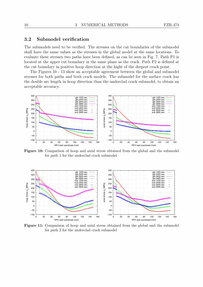
The submodels need to be verified. The stresses on the cut boundaries of the submodelshall have the same values as the stresses in the global model at the same locations. Toevaluate these stresses two paths have been defined, as can be seen in Fig. 7. Path P1 islocated at the upper cut boundary in the same plane as the crack. Path P2 is defined atthe cut boundary in positive hoop direction at the hight of the deepest crack point.

The Figures 10 - 13 show an acceptable agreement between the global and submodelstresses for both paths and both crack models. The submodel for the surface crack hasthe double arc length in hoop direction than the underclad crack submodel, to obtain anacceptable accuracy.

−100

−50

0

50

100

150

200

250

300

350

400

0 20 40 60 80 100 120 140 160

hoop

stre

ss σ

y [M

Pa]

RPV wall coordinate [mm]

glb 1200 sec.glb 2400 sec.glb 3600 sec.glb 3895 sec.sub 1200 sec.sub 2400 sec.sub 3600 sec.sub 3895 sec.

−100

−50

0

50

100

150

200

250

300

350

400

0 20 40 60 80 100 120 140 160

axia

l stre

ss σ

z [M

Pa]



Figure 10: Comparison of hoop and axial stress obtained from the global and the submodelfor path 1 for the underclad crack submodel

−100

−50

0

50

100

150

200

250

300

350

400

0 20 40 60 80 100 120 140 160

hoop

stre

ss σ

y [M

Pa]



−100

−50

0

50

100

150

200

250

300

350

400

0 20 40 60 80 100 120 140 160

axia

l stre

ss σ

z [M

Pa]



Figure 11: Comparison of hoop and axial stress obtained from the global and the submodelfor path 2 for the underclad crack submodel


−100

−50

0

50

100

150

200

250

300

350

400

0 20 40 60 80 100 120 140 160

hoop

stre

ss σ

y [M

Pa]



−100

−50

0

50

100

150

200

250

300

350

400

0 20 40 60 80 100 120 140 160

axia

l stre

ss σ

z [M

Pa]


glb 1200 sec.glb 2400 sec.glb 3600 sec.glb 3895 sec.

sub 1200 sec.sub 2400 sec.sub 3600 sec.sub 3895 sec.

Figure 12: Comparison of hoop and axial stress obtained from the global and the submodelfor path 1 for the surface crack submodel

−100

−50

0

50

100

150

200

250

300

350

400

0 20 40 60 80 100 120 140 160

hoop

stre

ss σ

y [M

Pa]



−100

−50

0

50

100

150

200

250

300

350

400

0 20 40 60 80 100 120 140 160

axia

l stre

ss σ

z [M

Pa]



Figure 13: Comparison of hoop and axial stress obtained from the global and the submodelfor path 2 for the surface crack submodel


3.3 Computation of stress intensity factors

For a crack loaded in mode I the stress intensity factor KI is related to the first componentof the j-integral J1. For a plane strain state the relation is

KI =

√J1E

1− ν2(3)

and for a plane stress state

KI =√

J1E. (4)

Here, E denotes the elastic modulus and ν Poisson’s ratio of the material.

3.3.1 The ANSYS kcalc method

A different approach is used by the ANSYS FE-code for elastic problems:

KI =√

2π2G

1 + κ

|uy|√r

, (5)

with the shear modulus G and stress state dependent κ

G =E

2(1 + ν), κ = 3− 4ν and κ =

3ν

1 + ν(6)

for plane strain and plane stress respectively. |uy| denotes the displacements perpendicularto the crack face for a model, which is symmetric to the ligament. r is the radial distancefrom the crack tip. Three pairs of |uy| and r are determined at node A located at the cracktip, and two nodes B and C, which are located at the crack face. The displacements arenormalized so that |uy| at node A is zero. Then two constants c1 and c2 are determinedso that

|uy|√r

= c1 + c2r (7)

at the nodes B and C. Then, let r approach 0

limr→0

|uy|√r

= c1 (8)

and Eq. 5 becomes

KI =√

2π2G

1 + κc1. (9)

The distances from the crack tip of the nodes B and C used to obtain |uy| are 3.75mmand 7.5mm for the underclad crack model and 7.5mm and 15mm for the surface crackmodel.


3.3.2 The VERLIFE method

The VERLIFE code gives a deterministic formula to estimate the stress intensity factor.

KI = σkY√

a (10)

This relation is also valid only for linear elastic cases. Here, σk is an effective stressmeasure obtained from the through wall distribution of the stress components normal tothe postulated crack face. For a surface crack the effective stress is

σk = 0.111 (3σA + σB + 5σc)

+ 0.4a

c(0.38σA − 0.17σB − 0.21σC)

− 0.28a

s

(1−

√a

c

)(σA − σB) (11)

and for an underclad crack

σk =σA + σC

2+

a

c· 4σA − 3σC − σB

30. (12)

The stress components σA, σB, and σC are calculated for the uncracked wall considering,however, the residual stresses in the weld. Y is a shape factor depending on the crackgeometry, which is for a surface crack

Y =2− 0.82a

c[1−

(0.89− 0.57

√ac

)3 (as

)1.5]3.25 (13)

and for an underclad crack

Y =1.79− 0.66a

c[1−

(a

b+a

)1.8(1− 0.4a

c− 0.8

{0.5− b+a

s

}0.4)]0.54 . (14)

The following table shows the geometric values, which are used to compute the stressintensity factor according to Eq. 10. The values for A, B and C are the distances fromthe inner vessel surface for the points where the normal stress components σA, σB andσC are obtained. s denotes the wall thickness, a and c the half crack width and length.Finally for the underclad crack, b is the distance of the point of the crack closest to thenearest surface from this surface, which is the length of the shorter ligament.

Table 5: Geometric values [mm] used to compute the stress intensity factor according to theVERLIFE code

value [mm] A B C a c s bunderclad crack 24 9 16.5 15 50 149 9

surface crack 24 0 12 24 50 149 -


3.3.3 The j-integral method

For the benchmark we will use the j-integral approach. For a two-dimensional case thefirst component of the j-integral is

J1 =

∫Γ

(wδj1 − σijui,1) njdΓ. (15)

Here, w denotes the strain energy density

w =

∫εij

σijdεij (16)

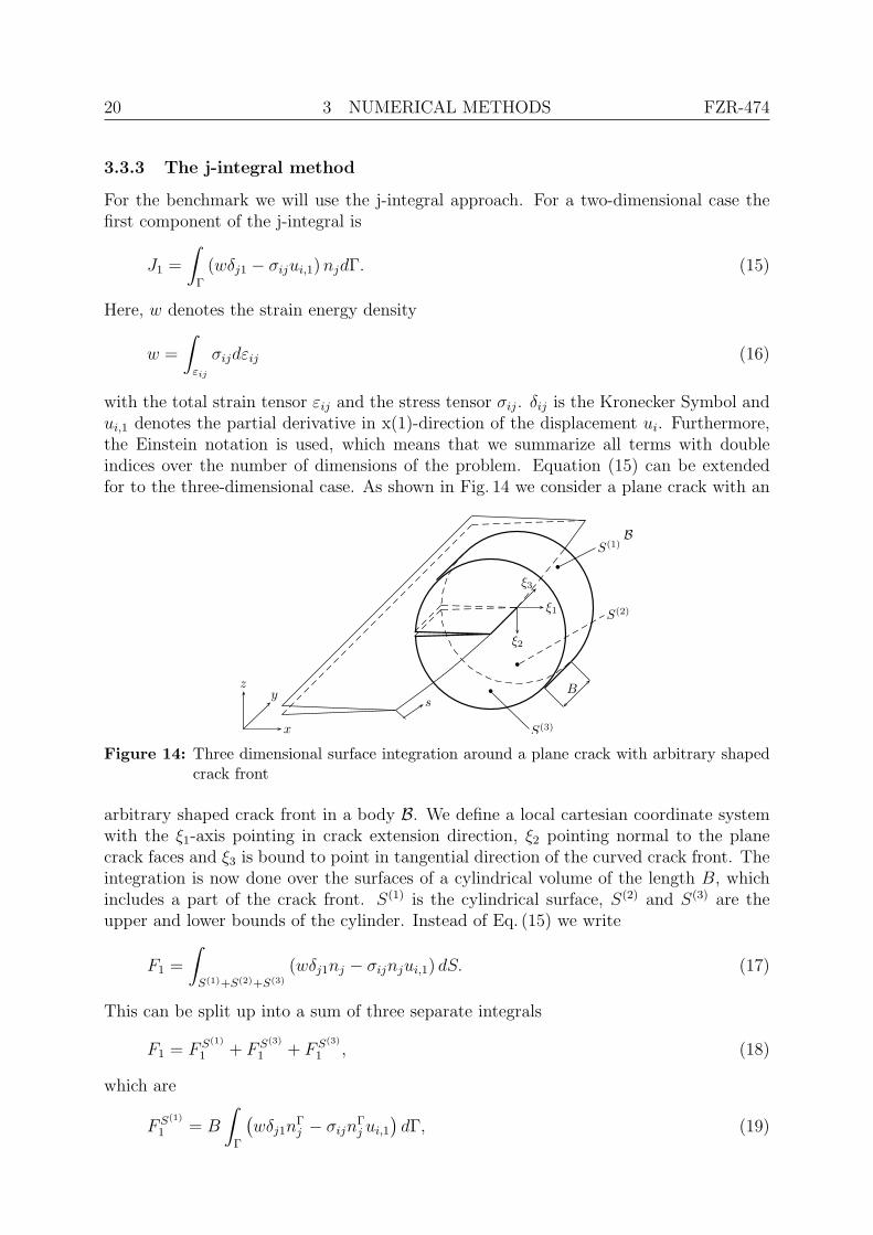
with the total strain tensor εij and the stress tensor σij. δij is the Kronecker Symbol andui,1 denotes the partial derivative in x(1)-direction of the displacement ui. Furthermore,the Einstein notation is used, which means that we summarize all terms with doubleindices over the number of dimensions of the problem. Equation (15) can be extendedfor to the three-dimensional case. As shown in Fig. 14 we consider a plane crack with an

B

x

yz

ξ1

ξ2

ξ3

sB

S(1)

S(2)

S(3)

Figure 14: Three dimensional surface integration around a plane crack with arbitrary shapedcrack front

arbitrary shaped crack front in a body B. We define a local cartesian coordinate systemwith the ξ1-axis pointing in crack extension direction, ξ2 pointing normal to the planecrack faces and ξ3 is bound to point in tangential direction of the curved crack front. Theintegration is now done over the surfaces of a cylindrical volume of the length B, whichincludes a part of the crack front. S(1) is the cylindrical surface, S(2) and S(3) are theupper and lower bounds of the cylinder. Instead of Eq. (15) we write

F1 =

∫S(1)+S(2)+S(3)

(wδj1nj − σijnjui,1) dS. (17)

This can be split up into a sum of three separate integrals

F1 = F S(1)

1 + F S(3)

1 + F S(3)

1 , (18)

which are

F S(1)

1 = B

∫Γ

(wδj1n

Γj − σijn

Γj ui,1

)dΓ, (19)


F S(2)

1 =

∫S(2)

(wδj1n

S(2)

j − σijnS(2)

j ui,1

)dS(2), (20)

F S(3)

1 =

∫S(3)

(wδj1n

S(3)

j − σijnS(3)

j ui,1

)dS(3). (21)

The outward normals on the three surfaces are

nΓj =

nΓ1

nΓ2

0

, nS(2)

j =

001

, nS(3)

j =

00−1

(22)

Now we let go B → 0 considering that nS(3)

j = −nS(2)

j and writing only S instead S(2) weget

J1 = limB→0

1

BF1 (23)

J1 =

∫Γ

(wδj1n

Γj − σijn

Γj ui,1

)dΓ +

∫S

(wδj1n

Sj − σijn

Sj ui,1

),3

dS. (24)

Considering further that the normal components nΓ3 = nS

1 = nS2 = 0 Eq. 24 becomes

J1 =

∫Γ

(wnΓ

1 − σijnΓj ui,1

)dΓ−

∫S

(σi3ui,1),3 dS. (25)

If we write all components we get

J1 =

∫Γ

(wnΓ

1

)dΓ

−∫

Γ

[(σ11n

Γ1 + σ12n

Γ2

)u1,1

]dΓ

−∫

Γ

[(σ21n

Γ1 + σ22n

Γ2

)u2,1

]dΓ

−∫

Γ

[(σ31n

Γ1 + σ32n

Γ2

)u3,1

]dΓ

−∫

S

(σ13u1,1 + σ23u2,1 + σ33u3,1),3 dS. (26)

If we take advantage of∫Γ

wnΓ1dΓ =

∫Γ

wdΓ2,

∫Γ

wnΓ2dΓ =

∫Γ

−wdΓ1, (27)


whereas dΓ1 and dΓ2 are the 1- and 2-component of the path increment dΓ, we get:

J1 =

∫Γ

wdΓ2

−∫

Γ

(σ11u1,1 + σ21u2,1 + σ31u3,1) dΓ2

−∫

Γ

(σ12u1,1 + σ22u2,1 + σ32u3,1) dΓ1

−∫

S

(σ13u1,1 + σ23u2,1 + σ33u3,1),3 dA. (28)

Eq. (28) needs to be extended if thermal strain fields, volumetric loads like gravity andtraction loads on the crack faces have to be considered.

J1 = Jmech1 + J th

1 − J bf1 − J cf

1 (29)

J th1 =

∫A(Γ)

σijεthij,1dA (30)

J bf1 =

∫A(Γ)

fiui,1dA (31)

J cf1 =

∫Γ(cf)

tiui,1dΓ(cf) (32)

Jmech1 is the classical mechanical part and equivalent to Eq. (26) and (28), J th

1 is thecorrection for thermal strains, J bf

1 is the correction for body forces or volumetric loadsand J cf

1 considers the crack face traction loads. A(Γ) is the cross section area of thecylinder bounded by circumferential path Γ and Γ(cf) is the path segment along the upperand lower crack face. If we assume an isotropic thermal expansion coefficient α and onlypressure loads p on the crack faces then we can simplify:

J th1 =

∫A(Γ)

(σ11 + σ12 + σ13) εth,1 dA, (33)

J bf1 =

∫A(Γ)

(f1u1,1 + f2u2,1 + f3u3,1) dA, (34)

J cf1 =

∫Γ(cf)

pu2,1 dΓ(cf). (35)


3.4 J-integral computation with ANSYS

We consider the following equation, which includes the correction terms for thermal fields,volumetric loads and crack face traction loads:

J1 =

∫Γ

(wδj1nj − σijnjui,1)dΓ

−∫

A(Γ)

(σijnjui,1),3dA(Γ)

+

∫A(Γ)

σijεthij,1dA(Γ)

−∫

A(Γ)

fiui,1dA(Γ)

−∫

Γ(cf)

pu2,1dΓ(cf) (36)

The value of J1 is theoretically independent from path Γ as long this path starts on

n2

B

ξ1

ξ2

Γ2 ΓA2 Γ1 Γ

A1

rA1

r1

rA2

r2

Γ+2

Γ−

2

Γ+1

Γ−

1

δw1

δw2

Figure 15: Integration scheme for two dimensional j-integral

a crack face, surrounds the crack tip and ends on the other crack face. If we considerplasticity J1 becomes path dependent if the outer integration contour (surface) passes theplastic zone [5]. For small scale yielding a path independent integral can be computed intwo dimensions if the integration path surrounds of the plastic zone. In three dimensionsthe integration boundary includes the top and bottom area S(1) and S(2) or A(Γ) ofthe cylindric integration boundary, which always crosses the crack tip, where plasticitycan occur. That is why a more or less significant path dependence will occur for threedimensional evaluations of J1 when plasticity occurs. Therefore, we compute J1 for severalpaths with increasing radius, to check if a saturation value of J1 can be reached. Brocksand Schneider [5] suggest to take the highest calculated J1 value with increasing domainsize as the closest to the real far field J1.

The different paths for the integral along Γl are concentric circles with increasing radii

rl = lrm

mfor l = 0 . . . m. (37)


The paths necessary for the area integration over A(Γ) have the radii

rAl =

rl + rl−1

2for l = 1 . . . m (38)

and the corresponding width

δwl = rl − rl−1 for l = 1 . . . m. (39)

The area integration with ANSYS is then a summation over path integrals along ΓAl that

are multiplied with their corresponding width.

Jm1 =

∫Γm

wn1dΓm

−∫

Γm

σijnjui,1dΓm

−m∑

l=1

∫ΓA

l

(σi3ui,1),3dΓAl δwl

+m∑

l=1

∫ΓA

l

σiiεth,1 dΓA

l δwl

−m∑

l=1

∫ΓA

l

fiui,1dΓAl δwl

+m∑

l=1

∫Γ+

l

pu2,1dΓ+l δwl

−m∑

l=1

∫Γ−l

pu2,1dΓ−l δwl (40)

Eq. (40) is computed with an ANSYS postprocessing tool, taking advantage of the pow-erful ANSYS path commands.

FZR-474 4 RESULTS 25

4 Results

The results requested by the benchmark are the variation of temperature, axial and hoopstress trough the RPV wall for the global model without a crack but at the position for theassumed crack. Furthermore, the variation of the stress intensity factors KI as a functionof the crack tip temperature for the deepest point of the crack and a position 2mm belowthe cladding-base material interface are required. Then the maximum allowable criticaltemperatures for both positions shall be provided. Additionally, we present the variationof KI along the crackfront for selected times.

4.1 Global model

The figures 16, 18 and 20 show data for a path across the RPV wall at the assumedcrack position for different times. The figures 17, 19 and 21 show the same data butplotted over time for different wall coordinates. In this plots, surface means the innerRPV surface, a=2mm is a point in the base material 2mm away from the cladding-basematerial interface and a=15mm is a point where the deepest point of the assumed crackwould be located. To be clear, there is no crack in the global model.

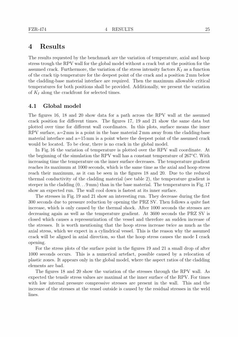
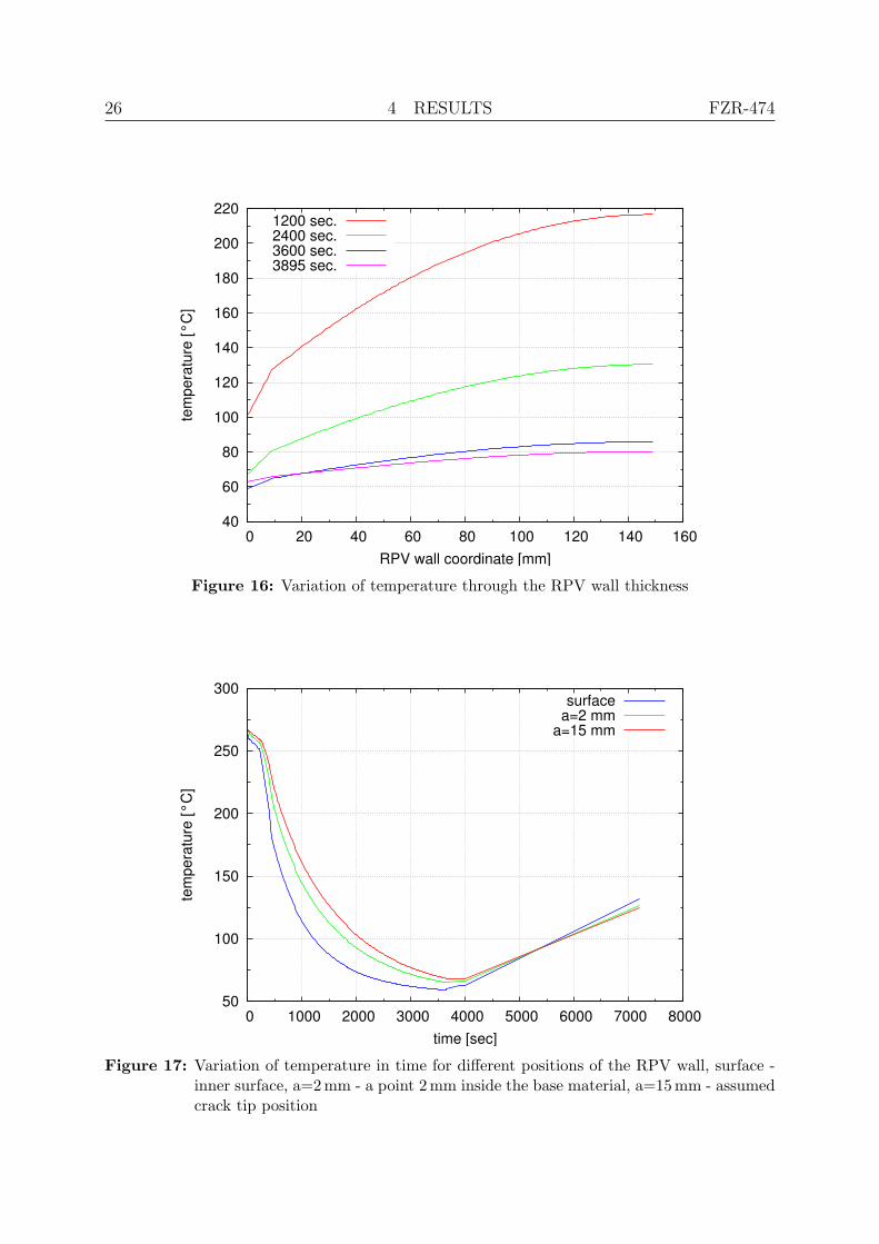
In Fig. 16 the variation of temperature is plotted over the RPV wall coordinate. Atthe beginning of the simulation the RPV wall has a constant temperature of 267◦C. Withincreasing time the temperature on the inner surface decreases. The temperature gradientreaches its maximum at 1000 seconds, which is the same time as the axial and hoop stressreach their maximum, as it can be seen in the figures 18 and 20. Due to the reducedthermal conductivity of the cladding material (see table 2), the temperature gradient issteeper in the cladding (0. . . 9mm) than in the base material. The temperatures in Fig. 17show an expected run. The wall cool down is fastest at its inner surface.

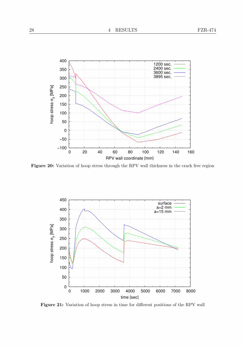
The stresses in Fig. 19 and 21 show an interesting run. They decrease during the first300 seconds due to pressure reduction by opening the PRZ SV. Then follows a quite fastincrease, which is only caused by the thermal shock. After 1000 seconds the stresses aredecreasing again as well as the temperature gradient. At 3600 seconds the PRZ SV isclosed which causes a repressurization of the vessel and therefore an sudden increase ofthe stresses. It is worth mentioning that the hoop stress increase twice as much as theaxial stress, which we expect in a cylindrical vessel. This is the reason why the assumedcrack will be aligned in axial direction, so that the hoop stress causes the mode I crackopening.

For the stress plots of the surface point in the figures 19 and 21 a small drop of after1000 seconds occurs. This is a numerical artefact, possible caused by a relocation ofplastic zones. It appears only in the global model, where the aspect ratios of the claddingelements are bad.

The figures 18 and 20 show the variation of the stresses through the RPV wall. Asexpected the tensile stress values are maximal at the inner surface of the RPV. For timeswith low internal pressure compressive stresses are present in the wall. This and theincrease of the stresses at the vessel outside is caused by the residual stresses in the weldlines.

26 4 RESULTS FZR-474

40

60

80

100

120

140

160

180

200

220

0 20 40 60 80 100 120 140 160

tem

pera

ture

[°C]


1200 sec.2400 sec.3600 sec.3895 sec.

Figure 16: Variation of temperature through the RPV wall thickness

50

100

150

200

250

300

0 1000 2000 3000 4000 5000 6000 7000 8000

tem

pera

ture

[°C]

time [sec]

surfacea=2 mm

a=15 mm

Figure 17: Variation of temperature in time for different positions of the RPV wall, surface -inner surface, a=2 mm - a point 2 mm inside the base material, a=15 mm - assumedcrack tip position


−100

−50

0

50

100

150

200

250

300

350

400

0 20 40 60 80 100 120 140 160

axia

l stre

ss σ

z [M

Pa]


1200 sec.2400 sec.3600 sec.3895 sec.

Figure 18: Variation of axial stress through the RPV wall thickness in the crack free region

0

50

100

150

200

250

300

350

400

450

0 1000 2000 3000 4000 5000 6000 7000 8000

axia

l stre

ss σ

z [M

Pa]

time [sec]

surfacea=2 mm

a=15 mm

Figure 19: Variation of axial stress in time for different positions of the RPV wall


−100

−50

0

50

100

150

200

250

300

350

400

0 20 40 60 80 100 120 140 160

hoop

stre

ss σ

y [M

Pa]


1200 sec.2400 sec.3600 sec.3895 sec.

Figure 20: Variation of hoop stress through the RPV wall thickness in the crack free region

0

50

100

150

200

250

300

350

400

450

0 1000 2000 3000 4000 5000 6000 7000 8000

hoop

stre

ss σ

y [M

Pa]

time [sec]

surfacea=2 mm

a=15 mm

Figure 21: Variation of hoop stress in time for different positions of the RPV wall


4.2 Underclad crack

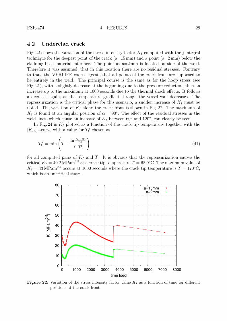
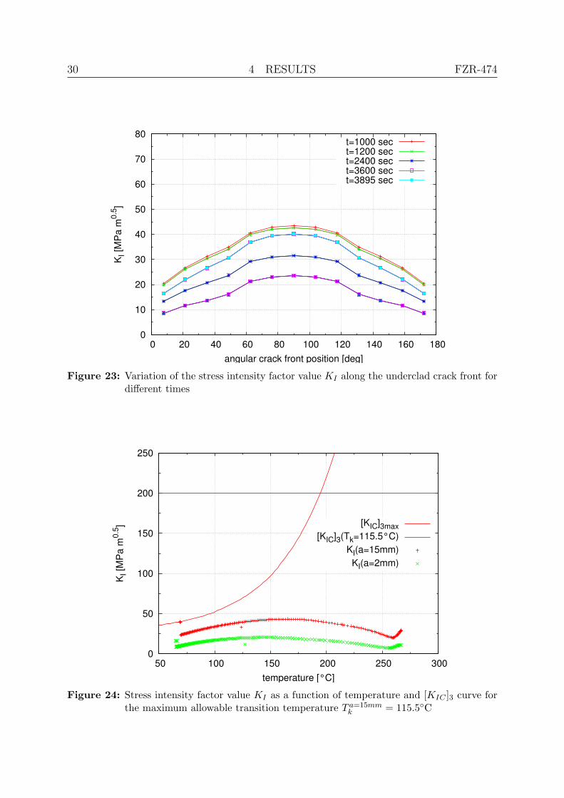
Fig. 22 shows the variation of the stress intensity factor KI computed with the j-integraltechnique for the deepest point of the crack (a=15mm) and a point (a=2mm) below thecladding-base material interface. The point at a=2mm is located outside of the weld.Therefore it was assumed, that in this location there are no residual stresses. Contraryto that, the VERLIFE code suggests that all points of the crack front are supposed tolie entirely in the weld. The principal course is the same as for the hoop stress (seeFig. 21), with a slightly decrease at the beginning due to the pressure reduction, then anincrease up to the maximum at 1000 seconds due to the thermal shock effects. It followsa decrease again, as the temperature gradient through the vessel wall decreases. Therepressurization is the critical phase for this scenario, a sudden increase of KI must benoted. The variation of KI along the crack front is shown in Fig. 22. The maximum ofKI is found at an angular position of α = 90◦. The effect of the residual stresses in theweld lines, which cause an increase of KI between 60◦ and 120◦, can clearly be seen.

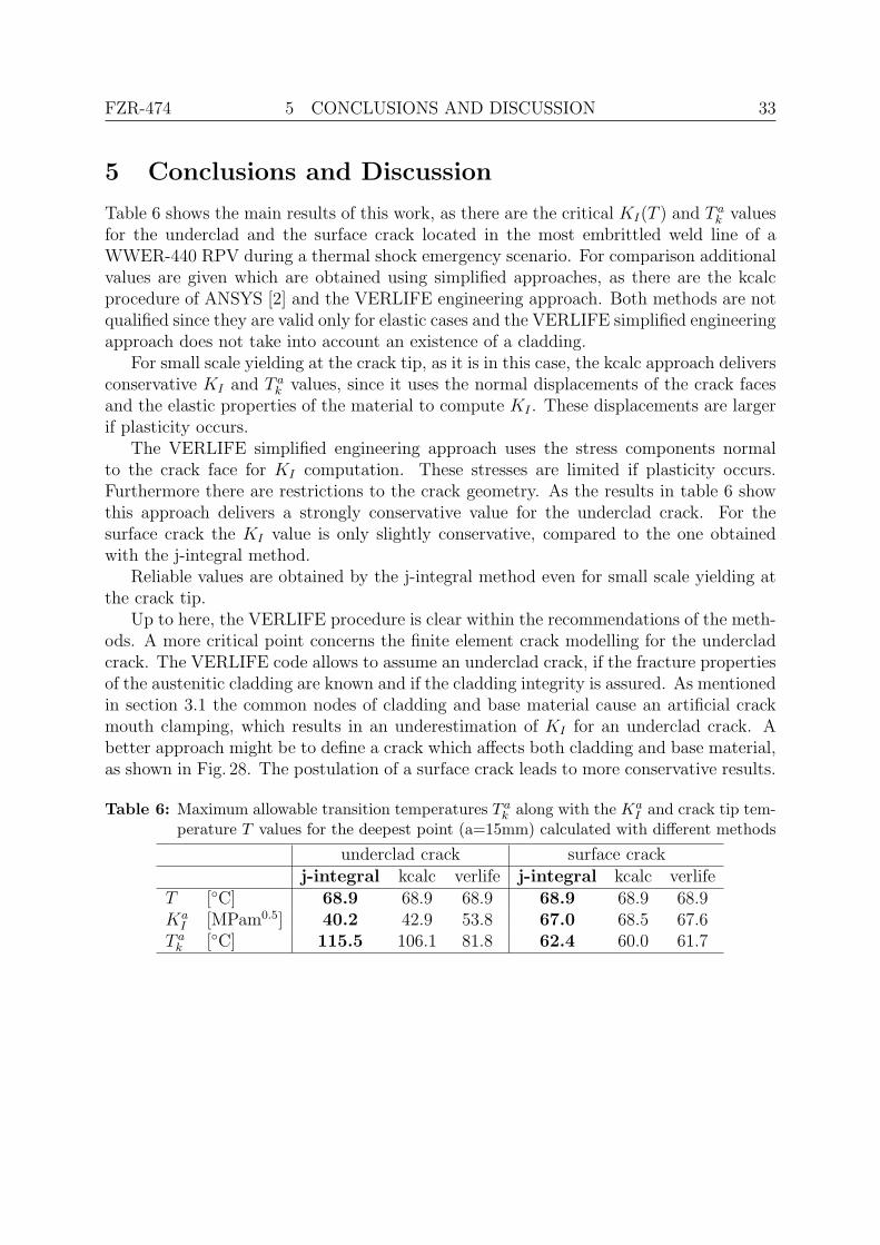
In Fig. 24 is KI plotted as a function of the crack tip temperature together with the[KIC ]3-curve with a value for T a

k chosen as

T ak = min

(T −

ln KI−2636

0.02

)(41)

for all computed pairs of KI and T . It is obvious that the repressurization causes thecritical KI = 40.2 MPam0.5 at a crack tip temperature T = 68.9◦C. The maximum value ofKI = 43 MPam0.5 occurs at 1000 seconds where the crack tip temperature is T = 170◦C,which is an uncritical state.

0

10

20

30

40

50

60

70

80

0 1000 2000 3000 4000 5000 6000 7000 8000

K I [M

Pa m

0.5 ]

time [sec]

a=15mma=2mm

Figure 22: Variation of the stress intensity factor value KI as a function of time for differentpositions at the crack front


0

10

20

30

40

50

60

70

80

0 20 40 60 80 100 120 140 160 180

K I [M

Pa m

0.5 ]

angular crack front position [deg]

t=1000 sect=1200 sect=2400 sect=3600 sect=3895 sec

Figure 23: Variation of the stress intensity factor value KI along the underclad crack front fordifferent times

0

50

100

150

200

250

50 100 150 200 250 300

K I [M

Pa m

0.5 ]

temperature [°C]

[KIC]3max[KIC]3(Tk=115.5°C)

KI(a=15mm)KI(a=2mm)

Figure 24: Stress intensity factor value KI as a function of temperature and [KIC ]3 curve forthe maximum allowable transition temperature T a=15mm

k = 115.5◦C


4.3 Surface crack

The results for the surface crack are in principle the same as for the underclad crack,but with elevated values of the stress intensity factors. Here also, the repressurizationof the RPV causes the critical value of KI = 67 MPam0.5 at a crack tip temperature ofT = 68.9◦C.

0

10

20

30

40

50

60

70

80

0 1000 2000 3000 4000 5000 6000 7000 8000

K I [M

Pa m

0.5 ]

time [sec]

a=15mma=2mm

Figure 25: Variation of the stress intensity factor value KI as a function of time for differentpositions at the crack front


0

10

20

30

40

50

60

70

80

0 20 40 60 80 100 120 140 160 180

K I [M

Pa m

0.5 ]

angular crack front position [deg]

t=1000 sect=1200 sect=2400 sect=3600 sect=3895 sec

Figure 26: Variation of the stress intensity factor value KI along the surface crack front fordifferent times

0

50

100

150

200

250

50 100 150 200 250 300

K I [M

Pa m

0.5 ]

temperature [°C]

[KIC]3max[KIC]3(Tk=62.36°C)[KIC]3(Tk=80.33°C)

KI(a=15mm)KI(a=2mm)

Figure 27: Stress intensity factor value KI as a function of temperature and [KIC ]3 curve forthe maximum allowable transition temperature T a=15mm

k = 62.36◦C, T a=2mmk =

80.33◦C

FZR-474 5 CONCLUSIONS AND DISCUSSION 33

5 Conclusions and Discussion

Table 6 shows the main results of this work, as there are the critical KI(T ) and T ak values

for the underclad and the surface crack located in the most embrittled weld line of aWWER-440 RPV during a thermal shock emergency scenario. For comparison additionalvalues are given which are obtained using simplified approaches, as there are the kcalcprocedure of ANSYS [2] and the VERLIFE engineering approach. Both methods are notqualified since they are valid only for elastic cases and the VERLIFE simplified engineeringapproach does not take into account an existence of a cladding.

For small scale yielding at the crack tip, as it is in this case, the kcalc approach deliversconservative KI and T a

k values, since it uses the normal displacements of the crack facesand the elastic properties of the material to compute KI . These displacements are largerif plasticity occurs.

The VERLIFE simplified engineering approach uses the stress components normalto the crack face for KI computation. These stresses are limited if plasticity occurs.Furthermore there are restrictions to the crack geometry. As the results in table 6 showthis approach delivers a strongly conservative value for the underclad crack. For thesurface crack the KI value is only slightly conservative, compared to the one obtainedwith the j-integral method.

Reliable values are obtained by the j-integral method even for small scale yielding atthe crack tip.

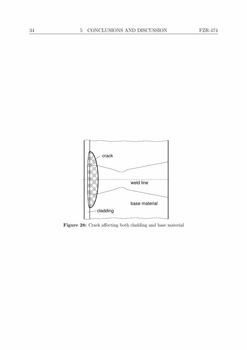
Up to here, the VERLIFE procedure is clear within the recommendations of the meth-ods. A more critical point concerns the finite element crack modelling for the undercladcrack. The VERLIFE code allows to assume an underclad crack, if the fracture propertiesof the austenitic cladding are known and if the cladding integrity is assured. As mentionedin section 3.1 the common nodes of cladding and base material cause an artificial crackmouth clamping, which results in an underestimation of KI for an underclad crack. Abetter approach might be to define a crack which affects both cladding and base material,as shown in Fig. 28. The postulation of a surface crack leads to more conservative results.

Table 6: Maximum allowable transition temperatures T ak along with the Ka

I and crack tip tem-perature T values for the deepest point (a=15mm) calculated with different methods

underclad crack surface crackj-integral kcalc verlife j-integral kcalc verlife

T [◦C] 68.9 68.9 68.9 68.9 68.9 68.9Ka

I [MPam0.5] 40.2 42.9 53.8 67.0 68.5 67.6T a

k [◦C] 115.5 106.1 81.8 62.4 60.0 61.7

34 5 CONCLUSIONS AND DISCUSSION FZR-474

� � � � � ��

� � � � � ��

��

��


weld line

crack

Figure 28: Crack affecting both cladding and base material

FZR-474 REFERENCES 35

References

[1] Eurotom Call 2004. VVER safety research. Technical report, Sixth Framework Pro-gramme Euratom, Other Activities in the Field of Nulcear Technologies and Safety,2005.

[2] ANSYS 10.0. ANSYS 10.0 Documentation, 2005.

[3] B.R. Bass, R.H. Bryan, J.W. Bryson, and J.G. Merkle. Applications of energy-release-rate techniques to part-trough cracks in experimental pressure vessel. Journalof Pressure Vessel Technology, 104(4):308–316, 1982.

[4] B.R. Bass and J.W. Bryson. Energy release rate techniques for combined thermo-mechanical loading. International Journal of Fracture, 104(1):R3–R7, 1983.

[5] W. Brocks and I. Schneider. Numerical aspects of the path-dependence of thej-integral in incremental plasticity. internal report GKSS/WMS/01/08, GKSS-Forschungszentrum Geesthacht, 2001.

[6] M. Brumovsky. Unified procedure for lifetime assessment of components and pipingin WWER NPPs VERLIFE. Technical report, European Commision, 5th Euratomframework programme 1998–2002, 2003.

[7] C.P. Cherepanov. Crack propagation in continous media. Journal of Applied Math-ematics and Mechanics, 31(3):476–488, 1967.

[8] J.D. Eshelby. The continuum theory of lattice defects. Solid State Physics, 3:79–114,1965.

[9] M. Kikuchi, H. Miyamoto, and Y. Sakaguchi. Evaluation of three-dimensional j-integral of semielliptical surface crack in pressure vessel. In SMIRT 5, G7/2, 1979.

[10] V. Pistora and P. Kral. Evaluation of pressurized thermal shocks for VVER-440/213reactor pressure vessel in NPP dukovany. In Transactions of 17th InternationalConference on Structural Mechanics in Reactor Technology (SMIRT 17), Paper No.G01-3, 2003.

[11] J.R. Rice. A path-independent integral and the approximate solution of strain con-centration by notches and cracks. Journal of Applied Mechanics, 35:379–386, 1968.

[12] C.F. Shih, B. Moran, and T. Nakamura. Energy release rate along a three-dimensionalcrack front in a thermally stressed body. International Journal of Fracture, 30:79–102, 1986.

[13] J. Sievers and A. Hofler. Application of the j-integral concept to thermal shockloadings. Nuclear Engineering and Design, 96:287–295, 1986.

covers wp4 benchmark 1 - qucosa: startseite · covers wp4 benchmark 1 ... and 100 205 11.9 13.3 0.3...

Documents