Momentum and the Flow of Mass

1 Introduction:

So far we have restricted ourselves to considering systems consisting of discrete objects or point-like objects that have fixed amounts of mass. We shall now consider systems in which material flows between the objects in the system, for example we shall consider coal falling from a hopper into a moving railroad car, sand leaking from railroad car fuel, grain moving forward into a railroad car, and fuel ejected from the back of a rocket, In each of these examples material is continuously flows into or out of an object.

We have already shown that the total external force causes the momentum of a system to change,

!p

! d p!F total = system . (19.1.1)ext dt

We shall analyze how the momentum of the constituent elements our system change over a time interval [t,t + !t] , and then consider the limit as !t " 0 . We can then explicit calculate the derivative on the right hand side of Eq. (19.1.1) and Eq. (19.1.1) becomes

system lim ext

!F

!p !p! !pd (t + !t) # (t)total system system system lim (19.1.2)= = = .

dt !t"0 !t !t"0 !t

We need to be very careful how we apply this generalized version of Newton’s Second Law to systems in which mass flows between constituent objects. In particular, when we isolate elements as part of our system we must be careful to identify the mass !m of the material that continuous flows in or out of an object that is part of our system during the time interval !t under consideration.

We shall consider four categories of mass flow problems that are characterized by the momentum transfer of the material of mass !m .

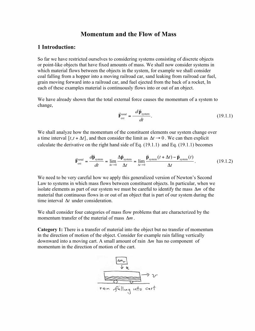
Category 1: There is a transfer of material into the object but no transfer of momentum in the direction of motion of the object. Consider for example rain falling vertically downward into a moving cart. A small amount of rain !m has no component of momentum in the direction of motion of the cart.

Category 2: The material continually leaves the object but it does not transport any momentum away from the object in the direction of motion of the object. For example, consider an ice skater gliding on ice holding a bag of sand that is leaking straight down with respect to the moving skater.

Category 3: The material continually hits the object providing an impulse resulting in a transfer of momentum to the object in the direction of motion. For example, suppose a fire hose is used to put out a fire on a boat. The incoming water continually hits the boat impulsing it forward.

Category 4: The material continually is ejected from the object, resulting in a recoil of the object. For example when fuel is ejected from the back of a rocket, the rocket recoils forward.

We must carefully identify the momentum of the object and the material transferred !m at time t in order to determine p! system (t) . We must also identify the momentum of the object and the material transferred !m at time t + !t in order to determine p! system (t + !t) as well. Recall that when we defined the momentum of a system, we assumed that the mass of the system remain constant. Therefore we cannot ignore the momentum of the transferred material at time t + !t even though it may have left the object, it is still part of our system (or at time t even though it has not flowed into the object yet).

2 Worked Examples

2.1 Worked Example Coal Car

An empty coal car of mass m0 starts from rest under an applied force of magnitude F . At the same time coal begins to run into the car at a steady rate b from a coal hopper at rest along the track. Find the speed when a mass mc of coal has been transferred.

Solution: We shall analyze the momentum changes in the horizontal direction which we call the x-direction. Because the falling coal does not have any horizontal velocity, the falling coal is not transferring any momentum in the x-direction to the coal car. So we shall take as our system the empty coal car and a mass mc of coal that has been transferred. Our initial state at t = 0 is when the coal car is empty and at rest before any coal has been transferred. The x-component of the momentum of this initial state is zero,

px (0) = 0 . (19.2.1)

Our final state at t = t f is when all the coal of mass mc = bt f has been transferred into the car that is now moving at speed v f . The x-component of the momentum of this final state is

px (t f ) = (m0 + mc )v f = (m0 + bt f )v f . (19.2.2)

There is an external constant force Fx = F applied through the transfer. The momentum principle applied to the x-direction is

t f

! Fxdt = "px = px (t f ) # px (0) . (19.2.3) 0

Since the force is constant, the integral is simple and the momentum principle becomes

Ft f = (m0 + bt f )v f . (19.2.4)

So the final speed is

Ft fv f (m + bt ) . (19.2.5) =

0 f

2.2 Worked Example: Emptying a Freight Car

A freight car of mass mc contains a mass of sand ms . At t = 0 a constant horizontal force of magnitude F is applied in the direction of rolling and at the same time a port in the bottom is opened to let the sand flow out at the constant rate b = dm s / dt . Find the speed of the freight car when all the sand is gone. Assume that the freight car is at rest at t = 0 .

Solution: Choose the positive x-direction to point in the direction that the car is moving. Let’s take as our system the amount of sand of mass !ms that leaves the freight car during the time interval [ , t t + !t] , and the freight car and whatever sand is in it at time t .

At the beginning of the interval the car and sand is moving with speed v so the x-component of the momentum at time t is given by

px (t) = (!ms + mc (t))v) , (19.2.6)

where mc ( ) t is the mass of the car and sand in it at time t . Denote by mc,0 = mc + ms where mc is the mass of the car and ms is the mass of the sand in the car at t = 0 , and ms ( ) t = bt is the mass of the sand that has left the car at time t since

t tdm ms (t) = ! dt

s dt = ! bdt = bt . (19.2.7) 0 0

Thus

mc (t) = mc,0 ! bt = mc + ms ! bt . (19.2.8)

During the interval [ , t t + !t] , the small amount of sand of mass !ms leaves the car with the speed of the car at the end of the interval v + !v . So the x-component of the momentum at time t + !t is given by

px (t + !t) = (!ms + mc (t))(v + !v) . (19.2.9)

Throughout the interval a constant force F is applied to the car so

px (t + !t) # px ( ) t . (19.2.10) F = lim !t"0 !t

From our analysis above Eq. (19.2.10) becomes

(mc ( ) t + !ms )( v + !v) # (mc ( ) t + !ms )v . (19.2.11) F = lim !t"0 !t

Eq. (19.2.11) simplifies to

s+ lim F = lim m ( ) t !v !m !v . (19.2.12) !t"0 c !t !t"0 !t

The second term vanishes when we take the !t " 0 because it is of second order in the infinitesimal quantities (in this case !ms!v ) and so when dividing by !t the quantity is of first order and hence vanishes since both !ms " 0 and !v " 0 . So Eq. (19.2.12) becomes

F = lim m ( ) t !v . (19.2.13) !t"0 c !t

We now use the definition of the derivative:

!v dv lim = (19.2.14) !t"0 !t dt

in Eq. (19.2.13) which then becomes the differential equation

dv F = mc ( ) t . (19.2.15) dt

Using Eq. (19.2.8) we have

dv F = (mc + ms ! bt ) . (19.2.16) dt

(b) We can integrate this equation through the separation of variable technique. Rewrite Eq. (19.2.16) as

Fdt . (19.2.17) dv = (mc + ms ! bt )

We can then integrate both sides of Eq. (19.2.17) with the limits as shown

v t ( ) t Fdt . (19.2.18) " dv = " m + m ! bt v=0 0 c s

Integration yields the velocity of the car as a function of time

v t ( ) = # F ln( mc + ms # bt ) t

0 = #

F ln !$ mc + ms # bt "

% . (19.2.19) b b & mc + ms '

2.3 Worked Example: Filling a Freight Car

Material is blown into cart A from cart B at a rate of b kilograms per second. The material leaves the chute vertically downward, so that it has the same horizontal velocity, u as cart B . At the moment of interest, cart A has mass mA and velocity v .

a) Define the objects that will constitute your system

b) Based on momentum flow diagrams, derive a differential equation for the velocity v . In particular find an expression for the rate of change of velocity, the instantaneous acceleration, dv / dt , of cart A .

Solution.

Define the system at time t to be the cart with whatever material is in it and the material blown into cart A during the time interval [t,t + !t] . Denote the mass of the cart and material at time t by mA and let !m denote the material blown into cart A during the time interval [t,t + !t] . At time t , cart A is moving with speed vA . At time t + !t Cart A is moving with speed vA + !vA . The momentum diagrams for time t and t + !t are shown below.

! ! There are no external forces acting on the system, Fext = 0 , so the momentum principle becomes

p! sys (t + !t) = p! sys (t) (2.20)

From our momentum flow diagram the x-component of the momentum is constant and equal to

(mA + !m)(vA + !vA ) = (mAvA + !mu) . (2.21)

Thus after rearranging

mA!vA + !m!vA = !m(u " vA ) . (2.22)

We can ignore the contribution form the second order term !m!vA , hence Eq. (2.22) becomes

mA!vA = !m(u " vA ) . (2.23)

Because the cart’s mass is increasing due to the material entering we have that

!m = !mA . (2.24)

and so Eq. (2.23) can now be written after taking limits as !t " 0

mAdvA = dmA (u ! vA ) . (2.25)

We can divide both sides of Eq. (2.25) by dt yielding

dvA dmAmA = (u ! vA ) . (2.26) dt dt

Rearranging terms and using the fact that the material is blown into the cart at a constant rate b ! dmA / dt , we have that the rate of change of the speed of the cart is given by

dvA b(u ! vA ) . (2.27) = dt mA

Extra:

We cannot directly integrate Eq. (2.27) with respect to dt because the mass of the cart is a function of time. In order to find the speed of the cart we need to know the relationship between the mass of the cart and the speed of the cart. There are two approaches.

In the first approach we separate variables in Eq. (2.25)

dvA dmA , (2.28) = u ! vA mA

and then integrate vA! = vA dvA

! mA! = mA dmA

! , (2.29) = ##

vA! =0 u " vA

! mA! = mA ,0

mA !

where mA,0 is the mass of the cart before any material has been blown in. After integration we have that

ln u mA= ln . (2.30)

u ! v mA A,0

Exponentiate both side gives u

= mA . (2.31)

u ! v mA A,0

We can solve this equation for the speed of the cart

m ! mv = A A,0 u . (2.32) A mA

Because the material is blown into the cart at a constant rate b ! dmA / dt , the mass of the cart as a function of time is given by

mA = mA,0 + bt . (2.33)

Therefore substituting Eq. (2.33) into Eq. (2.32) yields the velocity of the cart as a function of time is

bt u . (2.34) vA (t) = mA,0 + bt

In the second approach, we substitute Eq. (2.33) into Eq. (2.27) yielding

dvA b(u ! vA ) . (2.35) = dt m + btA,0

We can now separate variables

dvA = bdt

. (2.36) u ! v m + btA A,0

Now we can integrate vA! =vA (t ) t! = t

= # dvA

! dt! (2.37) #

u " v ! m + bt! vA! =0 A t! =0 A,0

yielding u m + bt

ln = ln A,0 . (2.38) u ! vA (t) mA,0

Again exponentiating both sides yields

u mA,0 + bt = . (2.39)

u ! vA (t) mA,0

and after some algebraic manipulation we can find the speed of the cart as a function of time

bt u . (2.40) vA (t) = mA,0 + bt

in agreement with Eq. (2.34).

3 Rocket Propulsion

A rocket at time t = 0 is moving with speed vr ,0 in the positive x-direction in empty space. The rocket burns fuel that is then ejected backward with velocity u ! relative to the rocket. This exhaust velocity is independent of the velocity of the rocket. The rocket must exert a force to accelerate the ejected fuel backwards and therefore by Newton’s Third law the fuel exerts a force that is equal in magnitude but opposite in direction resulting in propelling the rocket forward. The rocket velocity is a function of time, v ! r (t) , and increases at a rate dv ! / dt . Because fuel is leaving the rocket, the mass of the rocket is r

also a function of time, mr (t) , and is decreasing at a rate dm r / dt . We shall use the momentum principle, Eq. (19.1.2), to determine a differential equation that relates dv ! / dt , dm / dt , u ! , v ! (t) , and F

! total , an equation known as the rocket equation. r r r ext

Let t = ti denote the instant the rocket begins to burn fuel and let t = t f denote the instant the rocket has finished burning fuel. At some arbitrary time t during this process, the rocket has velocity v! r (t) ! v! r and the mass of the rocket is mr (t) ! mr . During the time interval [t,t + !t] , where !t is taken to be small (we shall eventually consider the limit that !t " 0 ), a small amount of fuel of mass !mf is ejected (in the limit that !t " 0 ,

!mf " 0 ) is ejected backwards with speed u ! relative to the rocket. The fuel was initially traveling at the speed of the rocket and so undergoes a change in momentum. Also the rocket recoils forward also undergoing a change in momentum. In order to keep track of all momentum changes, we define our system to be the rocket and the small amount of fuel that is ejected during the interval !t . At time t , the fuel has not yet been ejected so it is still inside the rocket. The figure below represents a momentum diagram at time for our system relative to a fixed inertial reference frame.

Momentum diagram for rocket a time t

The momentum of the system, p! system (t) , is therefore

p! system (t) = (mr + !mf )v!r . (19.3.1)

During the interval [t ,t + !t] the fuel is ejected backwards relative to the rocket with !v+ !

where !v! r represents the increase the rocket’s velocity. When the fuel element has completely left the rocket at the end of the time interval !t , the velocity of the rocket is v! r + !v! r , hence the velocity of the fuel relative to the fixed inertial reference frame is

!v (t + !t) = !vvelocity u! . The rocket recoils forward with an increased velocity r ,r r

!v+ !

figure below.

!v !v +!u . The momentum diagram of the system at time t + !t is shown in the = f r r

+ !

Momentum diagram for rocket a time t t!+

! ( )The momentum of the system is given by t t!p +system

!v

!v

(!v

Therefore the change in momentum of the system is given by

!v

! system

!v

+ !

! !

!p

!p (t + !t) = mr !v r ) + !mf (

!v r +!u) . (19.3.2)+ !system r r

!p !p(t + !t) " (t)=system system !v !v( + !r r r

!v !u)" (mr + !mf )!v .r) + !mf ( (19.3.3)= m +r r

!u+ !mf + !mf = m r r r

We can now apply Newton’s Second Law in the form of the momentum principle (Eq. (19.1.2)), for the system consisting of the rocket and exhaust fuel:

!p !p

!v

(t + !t) #!t

(t)!Fext

= lim

total system system = lim !t"0 !v!r r

!u!

!t"0 !t + !mf + !mfm r (19.3.4).

!v!!t"0 r !t !t"0 !t !t"0 !t

We note that !mf !v ! r is a second order differential, therefore

!!mf !v rlim = 0 . (19.3.5)

!t"0 !t We also note that

!v !m !m! !uf fr = lim + lim + lim m r

dv ! "v ! r r! lim , (19.3.6) dt "t#0 "t

and dmf "mf !! lim u . (19.3.7) dt "t#0 "t

Eq. (19.3.4) becomes

ext

!F

!v dmfdtotal !u (19.3.8)= m r + .r dt dt

The rate of decrease of the mass of the rocket, dmr / dt , is equal to the negative of the rate of increase of the exhaust fuel

dm dmfr = ! . (19.3.9) dt dt

Therefore substituting Eq. (19.3.9) into Eq. (19.3.8), we find that the differential equation describing the motion of the rocket and exhaust fuel is given by

d!v dm!Fext r

Eq. (19.3.10) is called the rocket equation.

!u .total (19.3.10)= m r ! r

dt dt

We shall first consider the case in which there are no external forces acting on the system, then Eq. (19.3.10) becomes

!vd dm = m r ! r !0

!u . (19.3.11)r dt dt

In order to solve this equation, we separate the variable quantities v ! r and mr

dv ! u ! dm r r . (19.3.12) = dt m dt r

We now multiply both sides by dt and integrate with respect to time between the initial time ti when the ejection of the burned fuel began and the final time t f when the process stopped.

t f dv ! t f u ! dm

dt = ! dt . (19.3.13) ! dtr

m dtr

ti ti r

We can rewrite the integrands and endpoints as

!v !u mr , fr , f

d!v dmr . (19.3.14) ! = !r m!vr ,i mr ,i r

Performing the integration and substituting in the values at the endpoints gives

ln mr , f . (19.3.15) !v !

!v =!ur , f r ,i m r ,i

Because the rocket is losing fuel, mr , f < mr ,i , we can rewrite Eq. (19.3.15) as

m ln r ,i . (19.3.16) !v !

!v = !!ur , f r ,i m r , f

!We note that v ! r and u point in opposite directions and hence have opposite signs. Also ln(mr ,i / mr , f ) > 1 . Therefore !v fr , >

!v r ,i as we expect.

After a slight rearrangement of Eq. (19.3.16), we have an expression for the velocity of the rocket as a function of the mass m of the rocket r

m ln r ,i (19.3.17) !v =

!v !!ur , f r ,i m r , f

Let’s examine our result. First, let’s suppose that all the fuel was burned and ejected. Then mr , f ! mr ,d is the final dry mass of the rocket (empty of fuel). The ratio

m R = r ,i (19.3.18)

m r ,d

is the ratio of the initial mass of the rocket (including the mass of the fuel) to the final dry mass of the rocket (empty of fuel). The final velocity of the rocket is then

!v r , f =!v r ,i !

!u ln R . (19.3.19)

If we want to write Eq. (19.3.19) in terms of speed, we denote the speeds by vr = v ! r and

u = u ! . Because v ! r and u ! point in opposite directions, in terms of speeds, Eq. (19.3.19) becomes

vr , f = vr ,i + u ln R . (19.3.20)

This is why multistage rockets are used. You need a big container to store the fuel. Once all the fuel is burned in the first stage, the stage is disconnected from the rocket. During the next stage the dry mass of the rocket is much less and so R is larger than the single stage, so the next burn stage will produce a larger final speed then if the same amount of fuel were burned with just one stage (more dry mass of the rocket).

In general rockets do not burn fuel at a constant rate but if we assume that

dmf dmb = = ! r (19.3.21)

dt dt

then we can integrate Eq. (19.3.21)

mr! = mr (t ) t != t

" dmr ! = #b " dt! (19.3.22) mr! = mr ,i t != ti

and find an equation that describes how the mass of the rocket changes in time

mr (t) = mr ,i ! b(t ! ti ) . (19.3.23)

For this special case, if we set t f = t in Eq. (19.3.17), then the velocity of the rocket as a function of time is given by

" m % r ,i!v r (t) =

!v r ,i !!u ln (19.3.24)$ ' .! bt# mr ,i &

3.1 Multi-Stage Rocket

(a) Before a rocket begins to burn fuel, the rocket has a mass of mr ,i = 2.81! 107 kg , of

which the mass of the fuel is mf ,i = 2.46 ! 107 kg . Then the dry mass of the rocket is

mr ,d ! mr ,i " mf ,i = 0.35 # 107 kg , hence R = mr ,i / mr ,d = 8.03 . The fuel is ejected at a speed u = 3000 m/s relative to the rocket. Starting from rest, the final change in speed of

the rocket after all the fuel has burned is !vr ,1 = u ln R = 6250 m/s . The single stage graph in the figure above shows the speed of the rocket as a function of time if the total burn time is 510 s and the fuel is burned at a constant rate.

(b) Now suppose that the same rocket burns the fuel in two stages ejecting the fuel in each stage at the same relative speed. In stage one, the available fuel to burn is mf ,1,i = 2.03 ! 107 kg with burn time 150 s . Then the mass of the rocket after all the fuel

in stage 1 one is burned is mr ,1,d = mr ,1,i ! mf ,1,i = 0.78 " 107 kg and

R1 = mr ,1,i / mr ,1,d = 3.60 . The change in speed after stage one is complete is

!vr ,1 = u ln R1 = 3840 m/s . Then the empty fuel tank and accessories from stage one are disconnected from the rest of the rocket. These disconnected parts had a mass m = 1.4 ! 106 kg , hence the remaining mass of the rocket is mr ,2,d = 2.1! 106 kg . All the

remaining fuel with mass mf ,2,i = 4.3 ! 106 kg is burned during stage 2 with burn time of

360 s . The mass of the rocket plus the unburned fuel is mr ,2,i = 6.4 ! 106 kg . Then

R2 = mr ,2,i / mr ,2,d = 3.05 . Therefore the rocket increases its speed during stage 2 by an

amount !vr ,2 = u ln R2 = 3340 m/s and the total change in speed after both stages is

!vr = u ln R1 + u ln R2 = u ln(R1R2 ) = 7190 m/s which is greater than if the fuel were burned in one stage. The two stage graph of the speed vs. time is shown also in the figure above.

3.2 Worked Example Rocket in a Constant Gravitational Field:

Now suppose that the rocket takes off from rest at time t = 0 in a constant gravitational field then the external force is

F!

total = m g ! (19.3.25) ext r

The momentum principle then becomes

d!v dm!g !u . (19.3.26)r ! rm = m dt dtr r

After rearranging Eq. (19.3.26) can be written as

d m !g!v !ud dt . (19.3.27) r += r m r

We now integrate both sides

!v t f

+ !mr , fr, f dm !gdt . (19.3.28) !v !ud r! !=r m!v 0 0mr ,i rr,i =

where mr ,i is the initial mass of the rocket and the fuel. Integration yields

" m % r ,i !gt . (19.3.29) !v r , f (t) = !

!u ln ' +$# mr , f &

After all the fuel is burned at t = t f , the mass of the rocket is equal to the dry mass

mr , f = mr ,d and so

!v r , f (t) = !!u ln R +

!gt . (19.3.30)

The first term on the right hand side is independent of the burn time. However the second term depends on the burn time. Because the direction of g ! and u ! are opposite the

direction of v ! r , f , the shorter the burn time, the smaller the vector contribution from the

third turn and hence the larger the final speed. So the rocket engine should burn the fuel as fast as possible in order to obtain the maximum possible speed.

MIT OpenCourseWare http://ocw.mit.edu

8.01SC Physics I: Classical Mechanics

For information about citing these materials or our Terms of Use, visit: http://ocw.mit.edu/terms.